Unbalanced minibatch Optimal Transport; applications to Domain Adaptation

Abstract

Optimal transport distances have found many applications in machine learning for their capacity to compare non-parametric probability distributions. Yet their algorithmic complexity generally prevents their direct use on large scale datasets. Among the possible strategies to alleviate this issue, practitioners can rely on computing estimates of these distances over subsets of data, i.e. minibatches. While computationally appealing, we highlight in this paper some limits of this strategy, arguing it can lead to undesirable smoothing effects. As an alternative, we suggest that the same minibatch strategy coupled with unbalanced optimal transport can yield more robust behavior. We discuss the associated theoretical properties, such as unbiased estimators, existence of gradients and concentration bounds. Our experimental study shows that in challenging problems associated to domain adaptation, the use of unbalanced optimal transport leads to significantly better results, competing with or surpassing recent baselines.

1 Introduction

Computing distances between distributions is a fundamental problem in machine learning. As an example, considering the space of distributions $\mathcal{M}_{+}(\mathcal{X})$ over a space $\mathcal{X}$, and given an empirical distribution $\alpha\in\mathcal{M}_{+}(\mathcal{X})$, many machine learning problems amount to estimate a distribution $\beta_{\lambda}$ parametrized by a vector $\lambda$ which approximates the distribution $\alpha$. In order to compute the dissimilarities between distributions, it is common to rely on a contrast function or divergence $L:\mathcal{M}_{+}(\mathcal{X})\times\mathcal{M}_{+}(\mathcal{X})\to\mathbb{R}_{+}$. In this setting, the goal is to find the optimal $\lambda^{*}$ which minimizes the distance $L$ between the distributions $\beta_{\lambda}$ and $\alpha$, i.e. $\lambda^{*}=\operatorname{argmin}_{\lambda}L(\alpha,\beta_{\lambda})$. As the available distributions are mostly empirical and come from data, the function $L$ needs good statistical estimation properties and optimization guarantees when using modern optimization techniques. Optimal transport (OT) losses have emerged recently as a competitive loss candidate for generative models (Arjovsky et al., 2017; Genevay et al., 2018). It also proved to be competitive in the context of Domain Adaptation (Courty et al., 2017, 2017; Shen et al., 2018) or for missing data imputation (Muzellec et al., 2020). The corresponding estimator is usually found in the literature under the name of Minimum Kantorovich Estimator (Bassetti et al., 2006; Peyré & Cuturi, 2019). However the computation of OT losses is a challenging problem, its computational cost being of order $\mathcal{O}(n^{3}log(n))$, where $n$ is the number of samples. Variants and approximations of optimal transport have been proposed to reduce its complexity. One of the most popular consists in adding an entropic regularization (Cuturi, 2013), leading to the Sinkhorn algorithm with complexity $\tilde{\mathcal{O}}(n^{2})$ in both space and time. However, when $n$ is large, computing OT remains rather expensive and might not fit on GPUs. The KeOps package (Feydy et al., 2019) allows to overcome this difficulty and avoid overflows by storing operations as formulas and stream computation on the fly. It is still difficult to use it in deep learning applications which involves high dimensional data and repeated computations of gradients. Another approach is to focus on the Wasserstein-1 distance which has a nice reformulation but needs to approximate 1-Lipschitz functions, which meets some difficulties in practice (Arjovsky et al., 2017; Gulrajani et al., 2017).

Minibatch Optimal Transport. A straightforward and scalable approach consists in computing OT solutions over subsets (minibatches) of the original data ($\alpha$ and $\beta$) and averaging the results as a proxy for the original problem. Such idea stems from the need to scale OT in practice and was applied in several situations (Kolouri et al., 2016; Genevay et al., 2018; Damodaran et al., 2018; Liutkus et al., 2019). It was proven for generative models that minimizers of the minibatch loss converge to the true minimizer when the minibatch size increases (Bernton et al., 2019). There exists deviation bounds between the true OT loss and a single minibatch estimate (Sommerfeld et al., 2019). Finally, concentration bounds and optimization properties for averaged minibatch OT were exhibited in (Fatras et al., 2020, 2021). However, the gain in computation time is achieved at the expense of the quality of the final transport plan, which turns out to be notably less sparse, leading to undesired pairings between samples that would not be coupled with exact OT. Figure 1 illustrates this effect on a 2D toy example which shows that samples from the same cluster in the source probability can be coupled to two different clusters in the target. We propose to handle this problem by leveraging the theory of unbalanced OT and computing a more robust transport plan at the minibatch level.

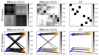
Figure 1: OT matrices, normalized by maximum value, between 2D distributions with $n=10$ samples. The first row shows the MBOT plans for different minibatch size $m$. The second row is the corresponding 2D visualization of the transport plan support.

Contributions and outline of the paper. We study in this work an alternative formulation of the minibatch OT where the unbalanced OT program, a variant with relaxed marginal constraints (Liero et al., 2017), is used at the minibatch level. Our rationale is that a geometrically robust version of OT computed between minibatches decreases the influence of undesired couplings between samples. The benefits of unbalanced MBOT are twofold: i) it yields a loss function more robust to minibatch sampling effects ii) our formulation approximates unbalanced OT but scales computationally w.r.t. the minibatch size, which allows its practical use for large datasets and deep learning applications. The contributions of the paper are the following. First we review the existing UOT formulations and introduce the one we consider in Section 2. We discuss the limits of minibatch OT in Section 3. We present the minibatch framework, study its statistical and optimization properties in Section 4. Finally, we design a new domain adaptation (DA) method whose performances are evaluated on several problems, where we show evidences that our strategy surpasses substantially other classical OT formulations, and is on par or better than recent state-of-the-art competitors. Our empirical results suggest that UOT might be more suitable than OT when dealing with real world data.

Notations. In this paper, we use the following notations. Let $\boldsymbol{X}=({\boldsymbol{x}}_{1},\cdots,{\boldsymbol{x}}_{n})$ (resp. $\boldsymbol{Y}=({\boldsymbol{y}}_{1},\cdots,{\boldsymbol{y}}_{n})$) be $n$ iid random vectors in ${\mathbb{R}}^{d}$ drawn from a distribution $\alpha$ (resp. $\beta$) on the source (resp. target) domain. We associate to $\{{\boldsymbol{x}}_{1},\cdots,{\boldsymbol{x}}_{n}\}$ and $\{{\boldsymbol{y}}_{1},\cdots,{\boldsymbol{y}}_{n}\}$ uniform vectors denoted $({\boldsymbol{u}}_{n})_{i}=(\frac{m_{\alpha}}{n})_{i}$, where $m_{\alpha}=\int d\alpha$ is the mass of $\alpha$. The quantities ${\boldsymbol{X}}$ and ${\boldsymbol{u}}_{n}$ allows one to recover an empirical distributions as $\alpha_{n}=\frac{1}{n}\sum_{i}\delta_{{\boldsymbol{x}}_{i}}$. We denote $\alpha^{\otimes m}$ for a sample of $m$ random variables following the distribution $\alpha$. The ground cost can be formalised as the following map:

$$C^{n}:({\boldsymbol{X}},{\boldsymbol{Y}})\mapsto\big{(}d({\boldsymbol{x}}_{i},{\boldsymbol{y}}_{j})\big{)}_{\small{1\leq i,j\leq n}}\in\mathcal{M}_{n}({\mathbb{R}}).$$ (1)

We further suppose that $\alpha$ and $\beta$ have compact support which means that the ground cost is bounded by a strictly positive constant $M$. This assumption holds for most machine learning applications where distributions are given by empirical samples.

2 Related work and background

We review in this section previous Unbalanced OT formulations, detail the one we consider in our approach and discuss the use of OT in robust machine learning.

Unbalanced Optimal Transport. Unbalanced OT is a generalization of ’classical’ OT that relaxes the conservation of mass constraints by allowing the system to either transport or create and destroy mass. Our loss builds upon (Liero et al., 2017) which replaces the ’hard’ marginal constraints of OT by ’soft’ penalties using Csiszàr divergences. There exists other extensions of the static formulations of OT. A famous one is partial OT which consists in transporting a fixed budget of mass (Figalli, 2010) or to move mass in and out of the system at a fixed cost (Figalli & Gigli, 2010). Another line of work proposes to optimize over various sets of Lipschitz functions (Hanin, 1992; Piccoli & Rossi, 2014; Schmitzer & Wirth, 2017). One can also replace Csiszàr divergences by integral probability metrics (Nath, 2020).

Consider a convex, positive, lower-semicontinuous function $\phi$ such that $\phi(1)=0$. Define $\phi^{\prime}_{\infty}=\lim_{x\rightarrow+\infty}\phi({\boldsymbol{x}})/{\boldsymbol{x}}$ that we suppose strictly positive. Csiszàr divergences $D_{\phi}$ are measures of discrepancy that compare pointwise ratios of mass using a penalty $\phi$ and are defined as $D_{\phi}({\boldsymbol{x}},{\boldsymbol{y}})=\sum_{{\boldsymbol{y}}_{i}\neq 0}{\boldsymbol{y}}_{i}\phi\Big{(}\frac{{\boldsymbol{x}}_{i}}{{\boldsymbol{y}}_{i}}\Big{)}+\phi^{\prime}_{\infty}\sum_{{\boldsymbol{y}}_{i}=0}{\boldsymbol{x}}_{i}$. Total Variation and Kullback-Leibler divergences ($\texttt{KL}({\boldsymbol{x}}|{\boldsymbol{y}})=\sum_{i}{\boldsymbol{x}}_{i}\log(\frac{{\boldsymbol{x}}_{i}}{{\boldsymbol{y}}_{i}})-{\boldsymbol{x}}_{i}+{\boldsymbol{y}}_{i}$) are particular instances of such divergence. Consider two positive distributions $\alpha,\beta\in\mathcal{M}_{+}(\mathcal{X})$. The UOT program between distributions and cost $c$ is defined as

$$\operatorname{OT}_{\phi}^{\tau,\varepsilon}(\alpha,\beta,c) =\underset{\pi\in\mathcal{M}_{+}(\mathcal{X}^{2})}{\text{min}}\int cd\pi+\varepsilon\texttt{KL}(\pi|\alpha\otimes\beta)$$

$$\quad\qquad{+\tau(D_{\phi}(\pi_{1}\|\alpha)+D_{\phi}(\pi_{2}\|\beta))},$$ (2)

where $\pi$ is the transport plan, $\pi_{1}$ and $\pi_{2}$ the plan’s marginals, $\tau$ is the marginal penalization and $\varepsilon\geq 0$ is the regularization coefficient. Note that the marginals of $\pi$ are no longer equal to $(\alpha,\beta)$ in general. The considered formulation is computable via a generalized Sinkhorn algorithm (Chizat et al., 2018; Séjourné et al., 2019) which is proved to converge. Its complexity for $D_{\phi}=\texttt{KL}$ is $\tilde{O}(n^{2}/\epsilon)$ (Pham et al., 2020). Balanced OT is recovered for inputs $(\alpha,\beta)$ with equal mass, when $\tau\rightarrow\infty$ (hence we note it $\operatorname{OT}_{\phi}^{\infty,0}$). When distributions are discrete, UOT can be expressed as $\operatorname{OT}_{\phi}^{\tau,\varepsilon}({\boldsymbol{a}},{\boldsymbol{b}},C)$ where ${\boldsymbol{a}}$ and ${\boldsymbol{b}}$ are two positive vectors, ${\boldsymbol{a}},{\boldsymbol{b}}\in\mathbb{R}_{+}^{n}$ and $C$ is the ground cost.

A shortcoming of adding entropy is the loss of metric properties since $\operatorname{OT}_{\phi}^{\tau,\varepsilon}(\beta,\beta,c)\neq 0$. It motivated (Séjourné et al., 2019) to introduce an unbalanced generalization of the Sinkhorn divergence (Genevay et al., 2018):

$$S_{\phi}^{\tau,\varepsilon}(\alpha,\beta,c) =\operatorname{OT}_{\phi}^{\tau,\varepsilon}(\alpha,\beta,c)+\frac{\varepsilon}{2}(m_{\alpha}-m_{\beta})^{2}$$ (3)

$$\quad-\frac{1}{2}\operatorname{OT}_{\phi}^{\tau,\varepsilon}(\alpha,\alpha,c)-\frac{1}{2}\operatorname{OT}_{\phi}^{\tau,\varepsilon}(\beta,\beta,c),$$

Computing the unbalanced sinkhorn divergence above is of the same order of complexity as the UOT loss. When $e^{-C/\epsilon}$ is a positive definite kernel, $S_{\phi}^{\tau,\varepsilon}$ is a convex, symmetric, positive definite loss function which metrizes the convergence in law (Séjourné et al., 2019). Thus it allows to mitigate between accelerated computations and conservation of key theoretical guarantees. Regarding empirical estimation, OT suffers from the curse of dimension which means that it is hard to estimate when data lie in high dimension $d$. Its sample complexity, i.e., its convergence in population, is proven to be in $O\left(\frac{1}{\sqrt{n}}\left(1+\frac{1}{\varepsilon^{\lfloor d/2\rfloor}}\right)\right)$ both for OT and UOT (Genevay et al., 2019; Séjourné et al., 2019).

Optimal Transport and robustness in machine learning. UOT is known to be more robust to outliers than OT as it does not need to meet the marginals. Several other formulations make optimal transport robust for practical and statistical reasons. Partial OT can be adapted for partial matchings problem with applications for positive-unlabeled learning (Chapel et al., 2020). A line of work proposes ’distributionnally robust’ models, where models are trained in a Wasserstein ball around the empirical distribution in the space of probabilities (Mohajerin Esfahani & Kuhn, 2018; Kuhn et al., 2019). In a similar approach, several variants relax the OT marginal constraints with a ball constraint, and consider several penalties such as integral probability metrics (Nath, 2020), total variation or Csiszàr divergences for outlier detection (Mukherjee et al., 2020; Balaji et al., 2020). Such relaxations allow to derive statistical guarantees w.r.t. noise and outliers. Another idea to ensure robustness consists in learning the cost adversarially, and is formulated as a max-min problem where the cost is modeled by an Euclidean embedding (Genevay et al., 2018), a compact space of matrices (Dhouib et al., 2020) or a projection on a lower dimensional subspace (Paty & Cuturi, 2019).

In the next section we discuss OT sensitivities in more details and highlight their exacerbation by minibatch strategy.

3 Minibatch OT and robustness to sampling

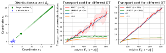
Figure 2: Several OT costs between 2D distributions with $n=10$ samples and $m=5$. Target distribution is equal to the source distribution tainted with a moving outlier (green dot). The shaded area represent the variance of subsample MBOT on 5 run (see section 4).

In this section, we discuss the limitations of combining balanced OT with the minibatch framework. OT is sensitive to the distributions geometry. When those distributions are tainted by outliers, OT is forced to transport them due to the marginal constraints, inducing an undesirable extra transportation cost. Minibatch OT averages several OT terms related to subsamples of the original distributions, thus sharing this sensitivity. The problem is even worse as two minibatches do not necessarily share samples that would lie in the support of the full OT plan, hence forced to match samples that could be, at the level of a minibatch, considered as outliers. Take as an example two distributions with clustered samples. While in the full OT plan clusters can be matched exactly, those clusters are likely to appear as imbalanced in the minibatches, especially if the size of the minibatch is small and does not respect the statistics of the original distribution. Due to the marginal constraints, samples from one cluster are likely to be matched to unrelated clusters, as depicted in Figure 1. This explains why in practice previous works relied on large minibatches to mitigate this sampling effect (Damodaran et al., 2018). To overcome this issue, we propose the natural solution of relaxing the marginal constraints at the minibatch level. The expected outcome is twofold: i) mitigating the effect of subsampling in the minibatch strategy and ii) providing a natural and scalable robust optimal transport computation strategy at the global level. We discuss in the following some theoretical considerations to support this claim.

Theoretical analysis: impact of an outlier

We start by examining the impact of an outlier in the behaviors of OT and UOT. The following lemma illustrates the relations between those two quantities.

Lemma 1.

Take $(\alpha,\beta)$ two probability distributions. For $\zeta\in[0,1]$, write $\tilde{\alpha}=\zeta\alpha+(1-\zeta)\delta_{\boldsymbol{z}}$ a distribution perturbed by a Dirac outlier located at some $z$ outside of the support of $(\alpha,\beta)$. Take the unregularized OT loss $\operatorname{OT}_{KL}^{\tau,0}$ with KL entropy and cost $C$. Write $m({\boldsymbol{z}})=\int C({\boldsymbol{z}},{\boldsymbol{y}})d\beta({\boldsymbol{y}})$. One has:

$$\operatorname{OT}_{\texttt{KL}}^{\tau,0}(\tilde{\alpha},\beta,C) \leq\zeta\operatorname{OT}_{\texttt{KL}}^{\tau,0}(\alpha,\beta,C)$$ (4)

$$+2\tau(1-\zeta)(1-e^{-m({\boldsymbol{z}})/2\tau})$$

Now take the unregularized, balanced OT loss $\operatorname{OT}_{\phi}^{\infty,0}$ with cost $C$. Write $(f,g)$ the optimal dual potentials (i.e. functions) of $\operatorname{OT}_{\phi}^{\infty,0}(\alpha,\beta)$, and $y^{*}$ in $\beta$’s support. Then:

$$\operatorname{OT}_{\phi}^{\infty,0}(\tilde{\alpha},\beta) \geq\zeta\operatorname{OT}_{\phi}^{\infty,0}(\alpha,\beta)$$ (5)

$$+(1-\zeta)\Big{(}C({\boldsymbol{z}},y^{*})-g(y^{*})+\int gd\beta\Big{)}$$

Equation (5) shows that when ${\boldsymbol{z}}$ gets further from the supports of $(\alpha,\beta)$, the OT loss increases. However for UOT the upper bound (4) tends to saturate as ${\boldsymbol{z}}$ gets further away. What remains is the UOT loss between distributions whose outliers are removed, with a cost of removing the outlier proportional to its mass.

We first illustrate Lemma 1 with a toy example in Figure 2. We consider a probability distribution $\alpha$ tainted with an outlier (green dot) to get a target probability distribution $\alpha^{\prime}=\frac{1}{n+1}(n.\alpha+\delta_{\boldsymbol{z}})$. We then move away the outlier from $\alpha$’s support, as shown with the green arrow, and we calculate several OT costs. The minibatch size is set to $m=5$ and the total cost is the average of $k$ OT costs between those minibatches. We see that OT variants are not robust to the outlier as their loss increases along the outlier displacement unlike UOT variants which reach a plateau as predicted by Lemma 1. Each computation is done 5 times to show that variance is lower for bigger $k$ and that UMBOT has a lower variance than MBOT for $k=30$ and $k=500$.

We consider now an example in 2D, akin to Figure 1, where our goal is to illustrate the OT plan between two empirical distributions of 10 samples in Figure 3. We use two 2D empirical distributions where the samples belong to a certain cluster depending on a related class (color information). The source data are equally distributed between classes while the target data have different proportions, 3 samples belong to the red class while 7 samples belong to the green class. Different proportions between domains are ubiquitous for real world data. We compare unbalanced minibatch OT, minibatch OT, entropic OT and UOT. For UOT, the divergence $D_{\phi}$ equals to KL divergence and for the minibatch variant, the minibatch size is $m=2$. We can see from the OT plans in the first row of the figure that the cluster structure is more or less recovered. However OT and minibatch OT tend to connect samples from different classes. This configuration would lead, for instance, to negative transfer in a context of domain adaptation applications, i.e., matching of samples between different domains. This is less true for UOT, where the pairings between different classes is diminished and tend to disappear when we reduce the penalty $\tau$.

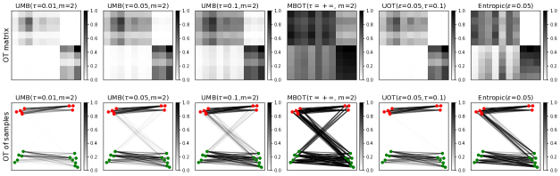
Figure 3: Several OT plans, normalized by their maximum value, between 2D distributions with $n=10$ samples. The first row shows the minibatch OT plans $\overline{\Pi}^{m}$ for different values of $m$, the second row provides an equivalent geometric interpretation of the OT plans, where the mass transportation is depicted as connexions between samples.

4 Unbalanced Minibatch Optimal Transport

In this section we express some mathematical properties at the heart of this work. In (Fatras et al., 2020), authors described some properties of the minibatch OT. We provide here extensions of those results to Unbalanced OT. We start by defining minibatch estimators, then we review the concentration bounds and finish with optimization properties. To derive concentration bounds we first prove that the UOT cost is finite and the optimal transport plan is bounded. Without loss of generality, we consider $n$-tuples ${\boldsymbol{X}}$ and ${\boldsymbol{Y}}$ with uniform vectors ${\boldsymbol{u}}_{n}$, to form empirical distributions encountered in the different applications and the associated ground cost matrix $C$.

4.1 Minibatch Unbalanced OT estimation

Estimators. To build minibatches, we select $m$ samples from ${\boldsymbol{X}}$ and ${\boldsymbol{Y}}$. We rely on a generic element of indices $I=(i_{1},\ldots,i_{m})\in\llbracket n\rrbracket^{m}$, which is called an index $m$-tuple. $I$ represents the selected samples from the $n$-data tuple ${\boldsymbol{X}}$ or ${\boldsymbol{Y}}$. In this work, we only focus on $m$-tuples without replacement $I$, whose their set is denoted ${\mathcal{P}^{m}}$.

Definition 1 (Minibatch UOT).

Let $C=C^{n}({\boldsymbol{X}},{\boldsymbol{Y}})$ be a square matrix of size $n$. Given an unbalanced OT loss $h\in\{\operatorname{OT}_{\phi}^{\tau,\varepsilon},S_{\phi}^{\tau,\varepsilon}\}$ and an integer $m\leq n$, we define the following quantity:

$$\bar{h}_{C}^{m}({\boldsymbol{X}},{\boldsymbol{Y}}):=\frac{(n-m)!^{2}}{n!^{2}}\sum_{I,J\in{\mathcal{P}^{m}}}h({\boldsymbol{u}}_{m},{\boldsymbol{u}}_{m},C_{I,J})$$ (6)

where for $I,J$ two $m$-tuples, $C_{(I,J)}$ is the matrix extracted from $C$ by keeping the rows and columns corresponding to $I$ and $J$ respectively. We denote the optimal plan $\Pi_{I,J}$, lifted as a $n\times n$ matrix where all entries are zero except those indexed in $I\times J$. We define the averaged minibatch transport plan: $\overline{\Pi}^{m}({\boldsymbol{X}},{\boldsymbol{Y}})\;\mathrel{\!\!{:}{=}\,}\dbinom{n}{m}^{-2}\sum_{I,J\in{\mathcal{P}^{m}}}\Pi_{I,J}.$

We omit $C$ when clear from context. A simple combinatorial argument provided in appendix assures that the sum of ${\boldsymbol{u}}_{m}$ over all $m$-tuples $I$ gives ${\boldsymbol{u}}_{n}$. In the formulation above, we no longer compute UOT between the full distributions but instead we compute the expectation of UOT over all minibatches drawn from $\alpha^{\otimes m}\otimes\beta^{\otimes m}$:

$$E_{h}\;\mathrel{\!\!{:}{=}\,}\underset{({\boldsymbol{X}},{\boldsymbol{Y}})\sim\alpha^{\otimes m}\otimes\beta^{\otimes m}}{\mathbb{E}}[h({\boldsymbol{u}}_{m},{\boldsymbol{u}}_{m},C^{m}({\boldsymbol{X}},{\boldsymbol{Y}}))],$$ (7)

The combinatorial number of terms is prohibitive to compute, fortunately we can rely on subsample quantities.

Definition 2 (Minibatch subsampling).

Consider the notations of definition 1. Pick an integer $k>0$, we define:

$$\widetilde{h}_{k,C}^{m}({\boldsymbol{X}},{\boldsymbol{Y}}):=k^{-1}\sum_{(I,J)\in D_{k}}h({\boldsymbol{u}}_{m},{\boldsymbol{u}}_{m},C_{I,J})$$ (8)

where $D_{k}$ is a set of cardinality $k$ whose elements are drawn at random from the uniform distribution on $\Gamma:=\mathcal{P}_{m}\times\mathcal{P}_{m}$. A similar construction holds for incomplete minibatch transport plan denoted as $\widetilde{\Pi}_{k}^{m}({\boldsymbol{X}},{\boldsymbol{Y}})$.

Note that $\bar{h}^{m}$ and $\widetilde{h}_{k}^{m}$ are unbiased estimators of $E_{h}$ as they are, respectively, complete and incomplete U-statistics (J Lee, 2019). The minibatch UOT losses are positive and symmetric, however they are not definites, i.e., $\bar{h}^{m}({\boldsymbol{X}},{\boldsymbol{X}})>0$ for non trivial ${\boldsymbol{X}}$ and $1<m<n$.

4.2 Deviation bounds

Our first lemma intends to show that the UOT cost is finite and that the optimal transport plan is bounded, which is needed to establish the concentration bounds.

Lemma 2 (Bounded UOT and optimal transport plan).

Let $C$ be a ground cost and ${\boldsymbol{a}},{\boldsymbol{b}}$ two positive vectors in ${\mathbb{R}}_{+}^{n}$ such that $m_{\boldsymbol{a}}=\|{\boldsymbol{a}}\|_{1}>0$ and $m_{\boldsymbol{b}}=\|{\boldsymbol{b}}\|_{1}>0$. Assume that $\langle{\boldsymbol{a}}{\boldsymbol{b}}^{\top},C\rangle<+\infty$. Consider $h=\operatorname{OT}_{\phi}^{\tau,\varepsilon}$ and assume $\varepsilon>0$ or $\phi^{\prime}_{\infty}>0$. Then $h({\boldsymbol{a}},{\boldsymbol{b}},C)$ is finite and the set of optimal transport plan is a compact set.

It is straightforward to prove boundedness of $h=S_{\phi}^{\tau,\varepsilon}$ from Lemma 2. We can now turn to establish concentration bounds for both incomplete estimators $\widetilde{h}_{k}^{m}$ and $\widetilde{\Pi}_{k}^{m}$.

Theorem 1 (Maximal deviation bound).

Let $\delta\in(0,1)$, three integers $k\geq 1$ and $m\leq n$ be fixed. Consider two $n$-tuples ${\boldsymbol{X}}\sim\alpha^{\otimes n}$ and ${\boldsymbol{Y}}\sim\beta^{\otimes n}$ and a kernel $h\in\{\operatorname{OT}_{\phi}^{\tau,\varepsilon},S_{\phi}^{\tau,\varepsilon}\}$. We have a maximal deviation bound between $\widetilde{h}_{k}^{m}({\boldsymbol{X}},{\boldsymbol{Y}})$ and $E_{h}$ depending on the number of samples $n$ and the number of batches $k$. With probability at least $1-\delta$ on the draw of ${\boldsymbol{X}},{\boldsymbol{Y}}$ and $D_{k}$ we have:

$$|\widetilde{h}_{k}^{m}({\boldsymbol{X}},{\boldsymbol{Y}})-E_{h}|\leq M\left(\sqrt{\frac{\log(\frac{2}{\delta})}{2\lfloor\frac{n}{m}\rfloor}}+\sqrt{\frac{2\log(\frac{2}{\delta})}{k}}\right),$$

where $M$ is the UOT upper bound. Furthermore, for $h=\operatorname{OT}_{\phi}^{\tau,\varepsilon}$, let $\mathfrak{M}_{\Pi}^{\infty}$ be the maximum mass of minibatch transport plans. For all $k\geqslant 1$, all $1\leqslant i\leqslant n$, with probability at least $1-\delta$ on the draw of ${\boldsymbol{X}},{\boldsymbol{Y}}$ and $D_{k}$ we have:

$$|\widetilde{\Pi}_{k}^{m}({\boldsymbol{X}},{\boldsymbol{Y}})_{(i)}\mathbf{1}_{n}-\overline{\Pi}^{m}({\boldsymbol{X}},{\boldsymbol{Y}})_{(i)}\mathbf{1}_{n}|\leqslant\mathfrak{M}_{\Pi}^{\infty}\sqrt{\frac{2\log(2/\delta)}{k}},$$

where we denote by $\Pi_{(i)}$ the $i$-th row of matrix $\Pi$ and by $\mathbf{1}_{n}\in{\mathbb{R}}^{n}$ the vector whose entries are all equal to $1$.

This deviation bound shows that if we increase the number of data $n$ and batches $k$ while keeping the minibatch size $m$ fixed, we get closer to the expectation. The rate $\frac{m}{n}$ is almost optimal and is the same as in (Fatras et al., 2020). The main difference is the upper bound $M$ which bounds UOT. Note that the bound does not depend on the dimension of $\mathcal{X}$ unlike original unbalanced OT (Séjourné et al., 2019). Regarding OT plans, the constant $\mathfrak{M}_{\Pi}$ represents the maximum mass of minibatch transport plans which would be 1 for OT.

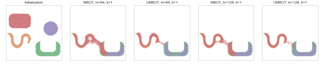
Figure 4: (Best viewed in colors) Minibatch UOT gradient flow on a 2D dataset. Source data and target data are divided in 2 imbalanced clusters, source left (red) and target right (green) shapes have 6400 samples while source right (purple) and target left (orange) shapes have 3600 samples. The batch size $m$ is set to $\{64,128\}$ and the number of minibatch $k$ is set to 1, meaning that the explicit Euler integration step is conducted for each batch. Results are computed with the (unbalanced) minibatch Sinkhorn divergence losses.

4.3 Unbiased gradients and optimization

The Wasserstein distance is known to suffer from biased gradients (Bellemare et al., 2017), meaning that minimizing the estimator of the Wasserstein distance with empiricial distributions does not lead to the minimum of the Wasserstein distance between full distribution. While minibatch entropic OT does not suffer from these biased gradients (Fatras et al., 2020), in this section we show that this property remains true for minibatch UOT, including unregularized UOT. We achieve this point by relying on Clarke regularity.

We study a standard parametric data fitting problem. Given some discrete samples $\left(x_{i}\right)_{i=1}^{n}\subset\mathcal{X}$ from an unknown distribution $\alpha$, our goal is to fit a parametric model $\lambda\mapsto\beta_{\lambda}\in\mathcal{M}_{+}(\mathcal{X})$ to $\alpha$ for $\lambda\in\Lambda$ in an Euclidian space. To do so, we use minibatch UOT and its incomplete estimators $\widetilde{h}_{k}^{m}$ as a contrast loss. U-statistics as contrast loss have been studied in (Papa et al., 2015). Stochastic gradients (SGD) has also proven to be really efficient at optimizing neural network parameters $\lambda$ even if they are non convex (Bottou, 2010). To justify the convergence of SGD, we need to exchange expectation and gradients and use that $\widetilde{h}_{k}^{m}$ is an unbiased estimator of $E_{h}$.

The former is not immediate because UOT is not differentiable as we do not have a unique optimal transport plan when $\varepsilon=0$. Thus, we use the notion of Clarke generalized derivatives. They define a regularity for nonsmooth but locally Lipschitz and semi-continuous function. It is a close concept to subgradients for convex functions since when a convex function is locally Lipshitz at ${\boldsymbol{x}}$ the two notions are equivalent. An intuitive geometric interpretation is that a function is Clarke regular if it doesn’t have ”upwards dashes” in its graph, for a total survey see (Clarke, 1990).

Theorem 2.

Let $\hat{{\boldsymbol{X}}},\{\hat{{\boldsymbol{Y}}}_{\theta}\}_{\theta\in\Theta}$ be two $m$-tuples of random vectors compactly supported, $h\in\{\operatorname{OT}^{\tau,\varepsilon},S^{\tau,\varepsilon}\}$ and $C^{m}$ a $\mathbf{C}^{1}$ cost. Under an additional integrability assumption, we have:

$$\partial_{\mathbf{\theta}}\mathop{\mathbb{E}}[h({\boldsymbol{u}},{\boldsymbol{u}},C^{m}(\hat{{\boldsymbol{X}}},\hat{{\boldsymbol{Y}}}_{\theta}))]=\mathop{\mathbb{E}}[\partial_{\mathbf{\theta}}h({\boldsymbol{u}},{\boldsymbol{u}},C^{m}(\hat{{\boldsymbol{X}}},\hat{{\boldsymbol{Y}}}_{\theta}))],$$

with both expectation being finite. Furthermore the function $\theta\mapsto-\mathop{\mathbb{E}}[h({\boldsymbol{u}},{\boldsymbol{u}},C^{m}(\hat{{\boldsymbol{X}}},\hat{{\boldsymbol{Y}}}_{\theta}))]$ is also Clarke regular.

Note that Theorem 2 implies that if we use the Minibatch UOT loss with $h\in\{\operatorname{OT}_{\phi}^{\tau,\varepsilon},S_{\phi}^{\tau,\varepsilon}\}$ as a loss function, then the minus objective function is Clarke regular. Furthermore, Stochastic gradient with decreasing step sizes converges almost surely to the set of critical points of Clarke generalized derivative (Davis et al., 2020; Majewski et al., 2018). As a consequence, it is justified to use SGD with minibatch UOT, as it converges to the optimal $\lambda^{*}$.

5 Experiments

In this section, we illustrate the practical behavior of unbalanced minibatch OT for gradient flow and for domain adaptation experiments. We relied on the POT package (Flamary & Courty, 2017) to compute the exact OT solver or the entropic UOT loss and the Geomloss package (Feydy et al., 2019) for the Unbalanced Sinkhorn divergence. The experiments were designed in PyTorch (Paszke et al., 2017) and all the code will be released upon publication.

5.1 Unbalanced MiniBatch OT gradient flow

Consider a given target distribution $\alpha$, the purpose of gradient flows is to model a distribution $\beta(t)$ which at each iteration follows the gradient direction minimizing the loss $\beta_{t}\mapsto h(\alpha,\beta_{t})$ (Peyré, 2015; Liutkus et al., 2019). The gradient flow simulate the non parametric setting of data fitting problem, where the modeled distribution $\beta$ is parametrized by a vector position ${\boldsymbol{x}}$ that encodes its support.

We follow the same experimental procedure as in (Feydy et al., 2019). The gradient flow algorithm uses a simple explicit Euler integration scheme. Formally, it starts from an initial distribution at time $t=0$ and integrates at each iteration a SDE. In our case, we cannot compute the gradient directly from our minibatch OT losses. As the OT loss inputs are empirical distributions, we have an inherent bias when we calculate the gradient from the weights $\frac{1}{m}$ of samples that we correct by multiplying the gradient by the inverse weight $m$. Finally, we integrate: $\dot{{\boldsymbol{X}}}(t)=-m\nabla_{\boldsymbol{{\boldsymbol{X}}}}\widetilde{h}_{k}^{m}({\boldsymbol{X}},{\boldsymbol{Y}})$.

For $\alpha$ and $\beta(0)$ we generate 10000 2D points divided in 2 imbalanced clusters with number of samples in each cluster provided in Figure 4. We consider the (unbalanced) sinkhorn divergence, a squared euclidean cost, a learning rate of 0.02, 5000 iterations, $m$ equals 64 or 128 and $k=1$. We show the gradient flow of the upper clusters to the lower clusters in Figure 4. From the experiment, we can see that the minibatch OT is not robust to imbalanced classes on the contrary to the minibatch UOT. Indeed there are data from the upper left cluster which converge to the down right cluster and we can also see an overlap between the classes. Due to OT marginal constraints, the loss forces to transport all data in the batch which results in breaking the target shapes. This is not the case for minibatch UOT, which better respects the shape of target distributions.

da	Method	A-C	A-P	A-R	C-A	C-P	C-R	P-A	P-C	P-R	R-A	R-C	R-P	avg
	resnet-50	34.9	50.0	58.0	37.4	41.9	46.2	38.5	31.2	60.4	53.9	41.2	59.9	46.1
	dann (*)	44.3	59.8	69.8	48.0	58.3	63.0	49.7	42.7	70.6	64.0	51.7	78.3	58.3
	cdan-e(*)	52.5	71.4	76.1	59.7	69.9	71.5	58.7	50.3	77.5	70.5	57.9	83.5	66.6
	deepjdot (*)	50.7	68.6	74.4	59.9	65.8	68.1	55.2	46.3	73.8	66.0	54.9	78.3	63.5
	alda (*)	52.2	69.3	76.4	58.7	68.2	71.1	57.4	49.6	76.8	70.6	57.3	82.5	65.8
	rot (*)	47.2	71.8	76.4	58.6	68.1	70.2	56.5	45.0	75.8	69.4	52.1	80.6	64.3
	jumbot	55.2	75.5	80.8	65.5	74.4	74.9	65.2	52.7	79.2	73.0	59.9	83.4	70.0
pda	resnet-50	46.3	67.5	75.9	59.1	59.9	62.7	58.2	41.8	74.9	67.4	48.2	74.2	61.4
	deepjdot(*)	48.2	66.2	76.6	56.1	57.8	64.5	58.3	42.7	73.5	65.7	48.2	73.7	60.9
	pada	51.9	67.0	78.7	52.2	53.8	59.0	52.6	43.2	78.8	73.7	56.6	77.1	62.1
	etn	59.2	77.0	79.5	62.9	65.7	75.0	68.3	55.4	84.4	75.7	57.7	84.5	70.4
	ba3us(*)	56.7	76.0	84.8	73.9	67.8	83.7	72.7	56.5	84.9	77.8	64.5	83.8	73.6
	jumbot	62.7	77.5	84.4	76.0	73.3	80.5	74.7	60.8	85.1	80.2	66.5	83.9	75.5

Table 1: Summary table of DA and Partial DA results on Office-Home (ResNet-50). (*) denotes the reproduced methods.

5.2 Domain adaptation

We now follow the settings of unsupervised DA where both domains share the same labels $\mathcal{Y}_{s}=\mathcal{Y}_{t}$.

jumbot. Optimal Transport has been proposed in (Courty et al., 2017) as a way to solve the domain adaptation problem. Our method is based on (Damodaran et al., 2018) and aims at finding a joint distribution map between a source and a target distribution by taking into account a term on a neural network embedding space and on the label space. Formally, let $g_{\theta}$ be an embedding function where the input is mapped into the latent space and $f_{\lambda}$ which maps the latent space to the label space on the target domain. The embedding space is in our experiment the before last layer of a neural network. For a given minibatch, embedding $g_{\theta}$ and classification map $f_{\lambda}$, the transfer term is:

$$\qquad\bar{h}_{C_{\theta,\lambda}}^{m}(({\boldsymbol{X}}^{s},{\boldsymbol{Y}}^{s}),({\boldsymbol{X}}^{t},f_{\lambda}(g_{\theta}({\boldsymbol{X}}^{t})))),\text{with }$$ (9)

$$(C_{\theta,\lambda})_{i,j}=\eta_{1}\|g_{\theta}({\boldsymbol{x}}_{i}^{s})-g_{\theta}({\boldsymbol{x}}_{j}^{t})\|_{2}^{2}+\eta_{2}\mathcal{L}({\boldsymbol{y}}_{i}^{s},f_{\lambda}(g_{\theta}({\boldsymbol{x}}_{j}^{t}))),$$

where $\mathcal{L}(.,.)$ is the cross-entropy loss and $\eta_{1},\eta_{2}$ are positive constants. Basically, this specific transportation cost combines a distance between the representation of the data through the neural network $g_{\theta}$ and a loss function between the associated labels (Courty et al., 2017). Taking $k=1$ led to state of the art results. The Csiszàr divergence $\phi$ is the Kullback-Leibler divergence KL. We also add a cross entropy term on the source data. Hence our optimization problem is:

$$\underset{\theta,\lambda}{\operatorname{min}} \sum_{i}\mathcal{L}(f_{\lambda}(g_{\theta}({\boldsymbol{x}}_{i}^{s})),{\boldsymbol{y}}_{i}^{s})$$ (10)

$$+\eta_{3}\widetilde{h}_{k,C_{\theta,\lambda}}^{m}(({\boldsymbol{X}}^{s},{\boldsymbol{Y}}^{s}),({\boldsymbol{X}}^{t},f_{\lambda}(g_{\theta}({\boldsymbol{X}}^{t})))).$$

Our method is called jumbot and stands for Joint Unbalanced MiniBatch OT. It is related to deepjdot (Courty et al., 2017; Damodaran et al., 2018) at the notable exceptions that we use minibatch UOT, which can also handle partial domain adaptation as suggested by our experiments.

Datasets. We start with digits datasets. Following the evaluation protocol of (Damodaran et al., 2018) we experiment on three adaptation scenarios: USPS to MNIST (U$\mapsto$M), MNIST to M-MNIST (M$\mapsto$MM), and SVHN to MNIST (S$\mapsto$M). MNIST (LeCun & Cortes, 2010) contains 60,000 images of handwritten digits, M-MNIST contains the 60,000 MNIST images with color patches (Ganin et al., 2016) and USPS (Hull, 1994) contains 7,291 images. Street View House Numbers (SVHN)(Netzer et al., 2011) consists of 73, 257 images with digits and numbers in natural scenes. We report the evaluation results on the test target datasets. Office-Home (Venkateswara et al., 2017) is a difficult dataset for unsupervised domain adaptation (UDA), it has 15,500 images from four different domains: Artistic images (A), Clip Art (C), Product images (P) and Real-World (R). For each domain, the dataset contains images of 65 object categories that are common in office and home scenarios. We evaluate all methods in 12 adaptation scenarios. VisDA-2017 (Peng et al., 2017) is a large-scale dataset for UDA from simulation to real. VisDA contains 152,397 synthetic images as the source domain and 55,388 real-world images as the target domain. 12 object categories are shared by these two domains. Following (Long et al., 2018; Chen et al., 2020), we evaluate all methods on VisDA validation set.

Methods/DA	U $\mapsto$ M	M $\mapsto$ MM	S $\mapsto$ M	Avg
dann(*)	92.2 $\pm$ 0.3	96.1 $\pm$ 0.6	88.7 $\pm$ 1.2	92.3
cdan-e(*)	99.2 $\pm$ 0.1	95.0 $\pm$ 3.4	90.9 $\pm$ 4.8	95.0
alda(*)	97.0 $\pm$ 1.4	96.4 $\pm$ 0.3	96.1 $\pm$ 0.1	96.5
deepjdot(*)	96.4 $\pm$ 0.3	91.8 $\pm$ 0.2	95.4 $\pm$ 0.1	94.5
jumbot	98.2 $\pm$ 0.1	97.0 $\pm$ 0.3	98.9 $\pm$ 0.1	98.0

Table 2: Summary table of DA results on digit datasets. Experiments were run three times. (*) denotes the reproduced methods.

Results. We compare our method against state of the art methods: dann(Ganin et al., 2016), cdan-e(Long et al., 2018), deepjdot(Damodaran et al., 2018), alda(Chen et al., 2020), rot(Balaji et al., 2020). Details about training procedure and architectures can be found in supplementary.

We reported the test score at the end of optimization for all benchmarks and methods. The results on digit datasets can be found in Table 2 where (*) denotes reproduced results. We conducted each experiment three times and report their average results and variance. For fair comparisons, we only resize and normalize the image without data augmentation. We see that our method performs best with a margin of at least $1.5$ points. Furthermore, we see an important $4\%$ increase of the performance compared to deepjdot. A deeper analysis of this difference is considered in the next paragraph. Office-Home results are gathered in Table 1 and VisDA are reported in Table 3. For fair comparison with previous work, we used a similar data pre-processing and we used the ten-crop technique (Long et al., 2018; Chen et al., 2020) for testing our methods. Experiments in (Balaji et al., 2020) follow a different setup explaining the difference of performance between their reported score and our reproduced score. jumbot achieves the best accuracy on average and on 11 of the 12 scenarios on the Office-Home dataset and achieves the best accuracy on VisDA at the end of training with a margin of 4% and 2% respectively.

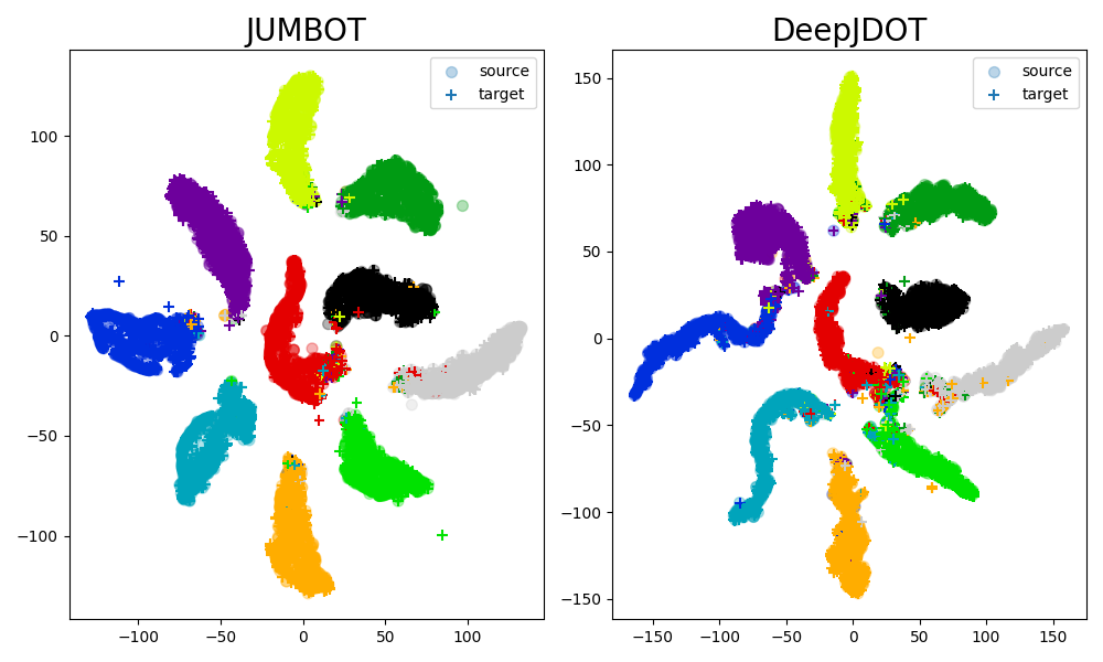
Figure 5: T-SNE embeddings of 10000 test samples for MNIST (source) and MNIST-M(target) for deepjdot and our method. It shows the ability of the methods to discriminate classes (samples are colored w.r.t. their classes).

Methods	Accuracy (in $\%$)
cdan-e(*)	70.1
alda(*)	70.5
deepjdot(*)	68.0
robust ot(*)	66.3
jumbot	72.5

Table 3: Summary table of DA results on VisDA datasets. (*) denotes the reproduced methods.

Analysis. In this paragraph, we study the difference of behavior between deepjdot and jumbot. Along jumbot’s training on the DA task USPS to MNIST, we measured the percentage of mass between data with different label at each iteration. In average along training about $7\%$ of deepjdot connections are between data with different labels while this percentage decreases to $0.7\%$ for jumbot. So deepjdot transfers wrong labels to the target which will decrease the overall accuracy. We also plot a TSNE embedding of our method and deepjdot (see Figure 5), we can see that there are some overlaps between clusters for deepjdot unlike our method. This is probably due to the minibatch smoothing effect which would tend to bring clusters of different classes closer. We provide in appendix a classification accuracy along training which demonstrates the network overfitting with deepjdot and not with jumbot. Finally, we also provide in supplementary a sensitivity analysis to the parameters, showing that jumbot is more robust to small batch size than deepjdot which is interesting for small computation budget.

5.3 Partial DA

Finally we consider the Partial DA (PDA) application. In PDA, the target labels are a subset of the source labels, i.e., $\mathcal{Y}_{t}\subset\mathcal{Y}_{s}$. Samples belonging to these missing classes become outliers which can produce negative transfer. We want to investigate the robustness of our method in such an extreme scenario. We evaluate our method on partial Office-Home, where we follow (Cao et al., 2018) to select the first 25 categories (in alphabetic order) in each domain as a partial target domain. We compare our method against state of the art PDA methods: pada (Cao et al., 2018), etn (Cao et al., 2019) and ba3us (Jian et al., 2020). For fair comparison we followed the experimental setting of pada, etn and ba3us and we report to the supplementary material for more details. The final performances are gathered in the lower part of table 1. Note that we do not use the ten-crop technics for evaluating the methods, as we were not able to reproduce pada and etn. We can see that jumbot is state of the art on 9 of the 12 domain adaptation tasks and is on average 2% above competitors. Finally, we also evaluate deepjdot (Damodaran et al., 2018) on the PDA task, jumbot is on average 15% higher on this problem despite the strong similar nature of the way the problem is solved, showing the clear advantages of our strategy.

6 Conclusion

Computing minibatches is a common practice to accommodate large quantities of data in deep learning, and can be used in synergy with OT. However it amplifies the shortcomings of OT due to its marginal constraints combined with subsampling effects, which is detrimental to learning application performances. To mitigate this issue, we propose to relax those constraints and use UOT at the minibatch level. We showed that not only theoretical properties are preserved with such loss, but it also dampens negative coupling effects, yielding a more efficient measure of comparison between data distributions. We notably showed it can reach state-of-the-art performances on challenging domain adaptation problems. We believe those results will encourage the use of minibatch Unbalanced OT in machine learning applications.

Acknowledgements

Authors would like to thank Younès Zine, Jérémy Cohen for fruitful discussions and Szymon Majewski for his proof checking. This work is partially funded through the projects OATMIL ANR-17-CE23-0012, OTTOPIA ANR-20-CHIA-0030 and 3IA Côte d’Azur Investments ANR-19-P3IA-0002 of the French National Research Agency (ANR). This research was produced within the framework of Energy4Climate Interdisciplinary Center (E4C) of IP Paris and Ecole des Ponts ParisTech. This research was supported by 3rd Programme d’Investissements d’Avenir ANR-18-EUR-0006-02. This action benefited from the support of the Chair ”Challenging Technology for Responsible Energy” led by l’X – Ecole polytechnique and the Fondation de l’Ecole polytechnique, sponsored by TOTAL.

Unbalanced minibatch Optimal Transport; applications to Domain Adaptation

Supplementary material

Outline.

The supplementary material of this paper is organized as follows:

• In section A, we first review the formalism with definitions and basic property proofs.

• In section B, we demonstrate our statistical and optimization results.

• In section C, we give extra experiments and details for domain adaptation experiments.

Appendix A Minibatch UOT formalism and basic properties

We start with the rigorous formalism of the minibatch UOT transport plan.

A.1 Minibatch UOT plan formalism

Definition 3.

We denote by $\operatorname{Opt}_{h}$ the set of all optimal transport plans for $h=\operatorname{OT}_{\phi}^{\tau,\varepsilon}$, cost matrix $C$ and a marginal ${\boldsymbol{u}}$. Let $\mathbf{u}_{m},\mathbf{u}_{m}\in(\mathbb{R}^{m})^{2}$ be discrete positive uniform vectors. For each pair of index $m$-tuples $I=(i_{1},\ldots,i_{m})$ and $J=(j_{1},\ldots,j_{m})$ from $\llbracket 1,n\rrbracket^{m}$, consider $C^{\prime}:=C_{I,J}$ the $m\times m$ matrix with entries $C^{\prime}_{k\ell}=C_{i_{k},j_{\ell}}$ and denote by $\Pi^{m}_{I,J}$ an arbitrary element of $\operatorname{Opt}_{h}$. It can be lifted to an $n\times n$ matrix where all entries are zero except those indexed in $I\times J$:

$$\Pi_{I,J} =Q_{I}^{\top}\Pi^{m}_{I,J}Q_{J}$$ (11)

where $$Q_{I} Q_{J} m\times n$$ and are matrices defined entrywise as

$$(Q_{I})_{ki} =\delta_{i_{k},i},1\leq k\leq m,1\leq i\leq n$$ (12)

$$(Q_{J})_{\ell j} =\delta_{j_{\ell},j},1\leq\ell\leq m,1\leq j\leq n.$$ (13)

Each row of these matrices is a Dirac vector, hence they satisfy $Q_{I}\mathbf{1}_{n}=\mathbf{1}_{m}$ and $Q_{J}\mathbf{1}_{n}=\mathbf{1}_{m}$.

We also define the averaged minibatch transport matrix which takes into account all possible minibatch couples.

Definition 4 (Averaged minibatch transport matrix).

Consider $h=\operatorname{OT}_{\phi}^{\tau,\varepsilon}$. Given data $n$-tuples ${\boldsymbol{X}},{\boldsymbol{Y}}$, consider for each pair of $m$-tuples $I$, $J$, the uniform vector of size $m,{\boldsymbol{u}}_{m}$, and let $\Pi_{I,J}$ be defined as in Definition 11.

The averaged minibatch transport matrix and its incomplete variant are :

$$\overline{\Pi}^{m}({\boldsymbol{X}},{\boldsymbol{Y}})\;\mathrel{\!\!{:}{=}\,}\frac{(n-m)!^{2}}{n!^{2}}\sum_{I\in{\mathcal{P}^{m}}}\sum_{J\in{\mathcal{P}^{m}}}\Pi_{I,J}.,$$ (14)

$$\widetilde{\Pi}_{k}^{m}({\boldsymbol{X}},{\boldsymbol{Y}}):=k^{-1}\sum_{(I,J)\in D_{k}}\Pi_{I,J},$$ (15)

where $D_{k}$ is a set of cardinality $k$ whose elements are drawn at random from the uniform distribution on $\Gamma:=\mathcal{P}_{m}\times\mathcal{P}_{m}$.

The average in the above definition is always finite so we do not need to concern ourselves with the measurability of selection of optimal transport plans. The same will be true whenever an average of optimal transport plans will be taken in the rest of this paper, since all results concerning such averages will be nonasymptotic. We will therefore avoid further mentioning this issue, for the sake of brevity. Unfortunately, on contrary to the balanced case, the minibatch UOT transport plan do not define OT transport plan as they do not respect the marginals, so in general the averaged minibatch UOT is not an OT transport plan. Note that the Sinkhorn divergence involves three terms, which explains why we can not define an associated averaged minibatch transport matrix.

A.2 Basic properties

Proposition 1 (Positivity, symmetry and bias).

The minibatch UOT are positive and symmetric losses. However, they are not definites, i.e., $\bar{h}^{m}({\boldsymbol{X}},{\boldsymbol{X}})>0$ for non trivial ${\boldsymbol{X}}$ and $1<m<n$.

Proof.

The first two properties are inherited from the classical UOT cost. Consider a uniform probability vector and random $3$-data tuple ${\boldsymbol{X}}=({\boldsymbol{x}}_{1},{\boldsymbol{x}}_{2},{\boldsymbol{x}}_{3})$ with distinct vectors $({\boldsymbol{x}}_{i})_{1\leq i\leq 3}$. As $\bar{h}^{m}$ is an average of positive terms, it is equal to 0 if and only if each of its term is 0. But consider the minibatch term $I_{1}=(i_{1},i_{2})$ and $I_{2}=(i_{1},i_{3})$, then obviously $h({\boldsymbol{u}},{\boldsymbol{u}},C({\boldsymbol{X}}(I_{1}),{\boldsymbol{X}}(I_{2})))\neq 0$ as ${\boldsymbol{x}}_{2}\neq{\boldsymbol{x}}_{3}$, where ${\boldsymbol{X}}(I_{1})$ denotes the data minibatch corresponding to indices in $I_{1}$. ∎

We now give the proof for our claim ”A simple combinatorial argument assures that the sum of ${\boldsymbol{u}}_{m}$ over all $m$-tuples $I$ gives ${\boldsymbol{u}}_{n}$.”

Proposition 2 (Averaged distributions).

Let ${\boldsymbol{u}}_{m}$ be a uniform vector of size $m$. The average over $m$-tuples $I\in{\mathcal{P}^{m}}$ for a given index of ${\boldsymbol{u}}_{m}$ is equal to $\frac{m_{\boldsymbol{a}}}{n}$, i.e., $\forall i\in\llbracket 1,n\rrbracket,\sum_{I\in{\mathcal{P}^{m}}}({\boldsymbol{u}}_{m})_{i}=({\boldsymbol{u}}_{n})_{i}=\frac{m_{\boldsymbol{a}}}{n}$.

Proof.

We recall that ${\mathcal{P}^{m}}$ denotes the set of all $m$-tuples without repeated elements. Let us check we recover the initial weights $({\boldsymbol{u}}_{n})_{i}=\frac{m_{\boldsymbol{a}}}{n}$. Observe that $\sum_{i=1}^{n}a_{i}=m_{\boldsymbol{a}}$ and that for each $1\leq i\leq n$

$$\sharp\{I\in{\mathcal{P}^{m}}:i\in I\} =\sharp\{I\in{\mathcal{P}^{m}}:n\in I\}$$

$$=\sharp\{I=(i_{1},\ldots,i_{m})\in{\mathcal{P}^{m}}:i_{1}=n\}+\ldots+\sharp\{I=(i_{1},\ldots,i_{m})\in{\mathcal{P}^{m}}:i_{m}=n\}$$

$$=m\cdot\sharp\{I=(i_{1},\ldots,i_{m})\in{\mathcal{P}^{m}}:i_{m}=n\}.$$ (16)

Since $\sharp\{I=(i_{1},\ldots,i_{m})\in{\mathcal{P}^{m}}:i_{m}=n\}$ is the number of $(m-1)$-tuples without repeated indices of $\llbracket 1,n-1\rrbracket$, $(n-1)!/(n-m)!$, it follows that

$$\frac{(n-m)!}{n!}\cdot\sum_{I\in{\mathcal{P}^{m}}}\frac{m_{\boldsymbol{a}}}{m}1_{I}(i) =\frac{(n-m)!}{n!}\sum_{I\in{\mathcal{P}^{m}},i\in I}\frac{m_{\boldsymbol{a}}}{m}=\frac{(n-m)!}{n!}\frac{m_{\boldsymbol{a}}}{m}\cdot\sharp\{I\in{\mathcal{P}^{m}}:i\in I\}$$ (17)

$$=\frac{(n-m)!}{n!}\frac{m_{\boldsymbol{a}}}{m}m\cdot\frac{(n-1)!}{(n-m)!}=\frac{m_{\boldsymbol{a}}}{n}$$ (18)

∎

Appendix B Proof main results

In this section we prove the UOT properties and the minibatch statistical and optimization theorems. We start with UOT properties as they are necessary to derive the minibatch results.

B.1 Unbalanced Optimal Transport properties

We recall the definition of Csiszàr divergences. Consider a convex, positive, lower-semicontinuous function such that $\phi(1)=0$. Define its recession constant as $\phi^{\prime}_{\infty}=\lim_{x\rightarrow+\infty}\phi({\boldsymbol{x}})/{\boldsymbol{x}}$. The Csiszàr divergence between positively weighted vectors $({\boldsymbol{x}},{\boldsymbol{y}})\in\mathbb{R}_{+}^{d}$ reads

$$D_{\phi}({\boldsymbol{x}},{\boldsymbol{y}})=\sum_{{\boldsymbol{y}}_{i}\neq 0}{\boldsymbol{y}}_{i}\phi\Big{(}\frac{{\boldsymbol{x}}_{i}}{{\boldsymbol{y}}_{i}}\Big{)}+\phi^{\prime}_{\infty}\sum_{{\boldsymbol{y}}_{i}=0}{\boldsymbol{x}}_{i}.$$

It allows to generalize OT programs. We retrieve common penalties such as Total Variation and Kullback-Leibler divergence by respectively taking $\phi({\boldsymbol{x}})=|{\boldsymbol{x}}-1|$ and $\phi({\boldsymbol{x}})=({\boldsymbol{x}}\log{\boldsymbol{x}}-{\boldsymbol{x}}+1)$. We provide a generalized definition of all OT programs as

$$\operatorname{OT}_{\phi}^{\tau,\varepsilon}({\boldsymbol{a}},{\boldsymbol{b}},C) =\underset{\Pi\in\mathbb{R}_{+}^{n\times n}}{\text{min}}\mathcal{F}(\Pi,C)=\underset{\Pi\in\mathbb{R}_{+}^{n\times n}}{\text{min}}\langle C,\Pi\rangle+\tau D_{\phi}(\Pi\mathbf{1}_{n}|{\boldsymbol{a}})+\tau D_{\phi}(\Pi^{T}\mathbf{1}_{n}|{\boldsymbol{b}})+\varepsilon\texttt{KL}(\Pi|{\boldsymbol{a}}\otimes{\boldsymbol{b}}).$$

Where $\mathcal{F}$ denotes the UOT energy.

B.1.1 Robustness

We start by showing the robustness properties lemma 1 that we split in two different lemmas. Lemma 1.1 shows that the UOT cost is robust to an outlier while lemma 1.2 shows that OT is not robust to an outlier.

Lemma 1.1.

Take $(\mu,\nu)$ two probability measures with compact support, and $z$ outside of $\nu$’s support. Recall the Gaussian-Hellinger distance (Liero et al., 2017) between two positive measures as

$$\operatorname{GH}_{\tau}(\mu,\nu)=\inf_{\pi\geq 0}\int C(x,y)d\pi(x,y)+\tau\texttt{KL}(\pi_{1}|\mu)+\tau\texttt{KL}(\pi_{2}|\nu).$$

For $\zeta\in[0,1]$, write $\tilde{\mu}=\zeta\mu+(1-\zeta)\delta_{z}$ a measure perturbed by a Dirac outlier. Write $m(z)=\int C(z,y)d\nu(y)$ One has

$$\operatorname{GH}_{\tau}(\tilde{\mu},\nu)\leq\zeta\operatorname{GH}_{\tau}(\mu,\nu)+2\tau(1-\zeta)(1-e^{-m(z)/2\tau})$$ (19)

In particular, with the notation $\operatorname{OT}_{\texttt{KL}}^{\tau,0}$ it reads

$$\operatorname{OT}_{\texttt{KL}}^{\tau,0}(\tilde{\mu},\nu,C) \leq\zeta\operatorname{OT}_{\texttt{KL}}^{\tau,0}(\mu,\nu,C)+2\tau(1-\zeta)(1-e^{-m({\boldsymbol{z}})/2\tau})$$

Proof.

Recall that the OT program reads

Write $\pi$ the optimal plan for $\operatorname{OT}_{\phi}^{\tau,0}(\mu,\nu)$. We consider a suboptimal plan for $\operatorname{OT}_{\phi}^{\tau,0}(\tilde{\mu},\nu)$ of the form

$$\tilde{\pi}=\zeta\pi+(1-\zeta)\kappa\delta_{z}\otimes\nu,$$

where $\kappa$ is mass parameter which will be optimized after. Note that the marginals of the plan $\tilde{\pi}$ are $\tilde{\pi}_{1}=\zeta\pi_{1}+(1-\zeta)\kappa\delta_{z}$ and $\tilde{\pi}_{2}=\zeta\pi_{2}+(1-\zeta)\kappa\nu$. Note that KL is jointly convex, thus one has

$$\texttt{KL}(\tilde{\pi}_{1}|\tilde{\mu}) \leq\zeta\texttt{KL}(\pi_{1}|\mu)+(1-\zeta)\texttt{KL}(\kappa\delta_{z}|\delta_{z}),$$

$$\texttt{KL}(\tilde{\pi}_{2}|\tilde{\mu}) \leq\zeta\texttt{KL}(\pi_{2}|\nu)+(1-\zeta)\texttt{KL}(\kappa\nu|\nu).$$

Thus a convex inequality yields

$$\operatorname{OT}_{\phi}^{\tau,0}(\tilde{\mu},\nu) \leq\zeta\Big{[}\int||x-y||d\pi(x,y)+\tau\texttt{KL}(\pi_{1}|\mu)+\tau\texttt{KL}(\pi_{2}|\nu)\Big{]}$$

$$+(1-\zeta)\Big{[}\kappa m(z)+\tau\texttt{KL}(\kappa\delta_{z}|\delta_{z})+\tau\texttt{KL}(\kappa\nu|\nu)\Big{]}.$$

We optimize now the upper bound w.r.t. $\kappa$. Both KL terms are equal to $\phi(\kappa)=\kappa\log\kappa-\kappa+1$, thus differentiating w.r.t. $\kappa$ yields

$$m(z)+2\tau\log\kappa=0\Rightarrow\kappa=e^{-m(z)/2\tau}.$$

Reusing this expression of $\kappa$ in the upper bound yields Equation (19). ∎

Lemma 1.2.

Take $(\mu,\nu)$ two probability measures with compact support, and $z$ outside of $\nu$’s support. Define the Wasserstein distance between two probabilities as

$$\operatorname{W}(\mu,\nu)=\sup_{f(x)+g(y)\leq C(x,y)}\int f(x)d\mu(x)+\int g(y)d\nu(y).$$ (20)

For $\zeta\in[0,1]$, write $\tilde{\mu}=\zeta\mu+(1-\zeta)\delta_{z}$ a measure perturbed by a Dirac outlier. Write $(f,g)$ the optimal dual potentials of $\operatorname{W}(\mu,\nu)$, and $y^{*}$ a point in $\nu$’s support. One has

$$\operatorname{W}(\tilde{\mu},\nu)\geq\zeta\operatorname{W}(\mu,\nu)+(1-\zeta)\Big{(}||z-y^{*}||^{2}-g(y^{*})+\int gd\nu\Big{)}$$ (21)

In particular, with the notation $\operatorname{OT}_{\texttt{KL}}^{\infty,0}$ it reads

$$\operatorname{OT}_{\phi}^{\infty,0}(\tilde{\mu},\nu) \geq\zeta\operatorname{OT}_{\phi}^{\infty,0}(\mu,\nu)+(1-\zeta)\Big{(}C({\boldsymbol{z}},y^{*})-g(y^{*})+\int gd\beta\Big{)}$$

Proof.

We consider a suboptimal pair $(\tilde{f},\tilde{g})$ of potentials for $\operatorname{OT}_{\phi}^{\infty,0}(\tilde{\mu},\nu)$. On the support of $(\mu,\nu)$ we take the optimal potentials pair $(f,g)$ for $(\mu,\nu)$, i.e. $\tilde{f}=f$ and $\tilde{g}=g$. We need to extend $\tilde{f}$ at $z$. To do so we take the $c$-transform of $g$, i.e.

$$\tilde{f}(z)=\inf_{y\in spt(\nu)}||z-y||^{2}-g(y)=||z-y^{*}||^{2}-g(y^{*}),$$

where the infimum is attained at some $y^{*}$ since $\nu$ has compact support. the pair $(\tilde{f},\tilde{g})$ is suboptimal, thus

$$\operatorname{OT}_{\phi}^{\infty,0}(\tilde{\mu},\nu) \geq\int\tilde{f}(x)d\tilde{\mu}(x)+\int\tilde{g}(y)d\nu(y)$$

$$\geq\zeta\int f(x)d\mu(x)+(1-\zeta)\tilde{f}(z)+\int\tilde{g}(y)$$

$$\geq\zeta\operatorname{OT}_{\phi}^{\infty,0}(\mu,\nu)+(1-\zeta)\Big{[}||z-y^{*}||^{2}-g(y^{*})+\int g(y)d\nu(y)\Big{]}$$

Hence the resulted given by Equation (21). ∎

B.1.2 UOT properties

Now let us present results which will be useful for concentration bounds. A key element is to have a bounded plan and a finite UOT cost in order to derive a hoeffding type bound. We start this section by proving lemma 2. We split it in two, lemma 2.1 proves that the UOT cost is finite and provides an upper bound while lemma 2.2 proves that the UOT plan exists and belongs to a compact set.

Lemma 2.1 (Upper bounds).

Let $({\boldsymbol{a}},{\boldsymbol{b}})$ be two positive vectors and assume that $\langle{\boldsymbol{a}}{\boldsymbol{b}}^{\top},C\rangle<+\infty$, then the UOT cost is finite. Furthermore, we have the following bound for $h=\operatorname{OT}_{\phi}^{\tau,\varepsilon}$, one has $|h({\boldsymbol{a}},{\boldsymbol{b}},C)|\leqslant M_{{\boldsymbol{a}},{\boldsymbol{b}}}^{h},$ where

$$M_{{\boldsymbol{a}},{\boldsymbol{b}}}^{h}=Mm_{\boldsymbol{a}}m_{\boldsymbol{b}}+\tau m_{\boldsymbol{a}}\phi(m_{\boldsymbol{b}})+\tau m_{\boldsymbol{b}}\phi(m_{\boldsymbol{a}}).$$ (22)

Regarding $h=S_{\phi}^{\tau,\varepsilon}$, one has $|h({\boldsymbol{a}},{\boldsymbol{b}},C)|\leqslant M_{{\boldsymbol{a}},{\boldsymbol{b}}}^{S},$ where

$$M_{{\boldsymbol{a}},{\boldsymbol{b}}}^{S}=2Mm_{\boldsymbol{a}}m_{\boldsymbol{b}}+\tau m_{\boldsymbol{a}}\phi(m_{\boldsymbol{b}})+\tau m_{\boldsymbol{b}}\phi(m_{\boldsymbol{a}})+\tau m_{\boldsymbol{a}}\phi(m_{\boldsymbol{a}})+\tau m_{\boldsymbol{b}}\phi(m_{\boldsymbol{b}})+\frac{\varepsilon}{2}(m_{\boldsymbol{a}}-m_{\boldsymbol{b}})^{2}.$$ (23)

Proof.

As $\langle{\boldsymbol{a}}{\boldsymbol{b}}^{\top},C\rangle<+\infty$ is finite, one can bound the ground cost $C$ as $0\leqslant C_{i,j}\leqslant M$. Consider the OT kernel $h\in\{\operatorname{OT}_{\phi}^{\tau,\varepsilon}\}$ for any $\varepsilon\geq 0$. Let us consider the transport plan $\Pi={\boldsymbol{a}}{\boldsymbol{b}}^{\top}=(a_{i}b_{j})$ (with respect to the cost matrix $C$). Because all terms are positive, we have:

$$|h| \leqslant\langle{\boldsymbol{a}}{\boldsymbol{b}}^{\top},C\rangle+\varepsilon\texttt{KL}({\boldsymbol{a}}{\boldsymbol{b}}^{\top}|{\boldsymbol{a}}{\boldsymbol{b}}^{\top})+\tau D_{\phi}\left(({\boldsymbol{a}}{\boldsymbol{b}}^{\top})\mathbf{1}_{n}|{\boldsymbol{a}}\right)+\tau D_{\phi}\left(({\boldsymbol{b}}{\boldsymbol{a}}^{\top})\mathbf{1}_{n}|{\boldsymbol{b}}\right)$$

$$\leqslant M\sum_{i,j}a_{i}b_{j}+\tau m_{\boldsymbol{a}}\phi(m_{\boldsymbol{b}})+\tau m_{\boldsymbol{b}}\phi(m_{\boldsymbol{a}})$$

$$\leqslant Mm_{\boldsymbol{a}}m_{\boldsymbol{b}}+\tau m_{\boldsymbol{a}}\phi(m_{\boldsymbol{b}})+\tau m_{\boldsymbol{b}}\phi(m_{\boldsymbol{a}})$$ (24)

Defining $M_{{\boldsymbol{a}},{\boldsymbol{b}}}^{h}$ as the last upper bound finishes the proof. The case $h=S_{\phi}^{\tau,\varepsilon}$, is the sum of three terms of the form $\operatorname{OT}_{\phi}^{\tau,\varepsilon}$ Thus the sum $M_{{\boldsymbol{a}},{\boldsymbol{b}}}^{h}+\tfrac{1}{2}M_{{\boldsymbol{a}},{\boldsymbol{a}}}^{h}+\tfrac{1}{2}M_{{\boldsymbol{b}},{\boldsymbol{b}}}^{h}$ is an upper bound of $S_{\varepsilon}$. ∎

We now bound the UOT plan.

Lemma 2.2 (locally compact optimal transport plan).

Assume that $\langle{\boldsymbol{a}}{\boldsymbol{b}}^{\top},C\rangle<+\infty$. Consider regularized or unregularized UOT with entropy $\phi$ and penalty $D_{\phi}$ such that one has $\phi^{\prime}_{\infty}>0$. Then there exists an open neigbhourhood $U$ around $C$, and a compact set $K$, such that the set of optimal transport plan for any $\tilde{C}\in U$ is in K, i.e., $\operatorname{Opt}_{h}(\tilde{C})\subset K$. Furthermore, if all costs are uniformly bounded such that $0\leq C\leq M<\infty$, then the compact K can be taken global, i.e. independent of $C$.

Proof.

We identify the mass of a positive measure with its L1 norm, i.e. $m_{\boldsymbol{a}}=\sum{\boldsymbol{a}}_{i}=||{\boldsymbol{a}}||_{1}$. We first consider the case where $0\leq C\leq M<\infty$. The OT cost is finite because the plan $\pi={\boldsymbol{a}}{\boldsymbol{b}}^{\top}$ is suboptimal and yields $\operatorname{OT}_{\phi}^{\tau,\varepsilon}({\boldsymbol{a}},{\boldsymbol{b}},C)\leq Mm_{\boldsymbol{a}}m_{\boldsymbol{b}}+\tau m_{\boldsymbol{a}}\phi(m_{\boldsymbol{b}})+\tau m_{\boldsymbol{b}}\phi(m_{\boldsymbol{a}})<+\infty$.

Take a sequence $\Pi_{t}$ approaching the infimum. Note that thanks to the Jensen inequality, one has $D_{\phi}({\boldsymbol{x}},{\boldsymbol{y}})\geq m_{\boldsymbol{y}}\phi(m_{\boldsymbol{x}}/m_{\boldsymbol{y}})$ (see (Liero et al., 2017)). Write $m_{\Pi}=\sum\Pi_{t,ij}$. One has for any $t$

$$\langle\Pi_{t},C\rangle +\tau D_{\phi}(\Pi_{t,1}\mathbf{1}_{n}|{\boldsymbol{a}})+\tau D_{\phi}(\Pi_{t,2}^{\top}\mathbf{1}_{n}|{\boldsymbol{b}})+\epsilon\textrm{KL}(\Pi_{t}|{\boldsymbol{a}}{\boldsymbol{b}}^{\top})$$

$$\geq m_{\Pi}\Bigg{[}\min C_{ij}+\tau\frac{m_{\boldsymbol{a}}}{m_{\Pi}}\phi\big{(}\frac{m_{\Pi}}{m_{\boldsymbol{a}}}\big{)}+\tau\frac{m_{\boldsymbol{b}}}{m_{\Pi}}\phi\big{(}\frac{m_{\Pi}}{m_{\boldsymbol{b}}}\big{)}+\varepsilon\frac{m_{\boldsymbol{a}}m_{\boldsymbol{b}}}{m_{\Pi}}\phi_{KL}\big{(}\frac{m_{\Pi}}{m_{\boldsymbol{a}}m_{\boldsymbol{b}}}\big{)}\Bigg{]}$$

$$\geq m_{\Pi}L(m_{\Pi}).$$

If $||\Pi_{t}||_{1}=m_{\Pi}\rightarrow+\infty$, then $L(m_{\Pi})\rightarrow+\infty$ if $\varepsilon>0$ and $L(m_{\Pi})\rightarrow\min C_{ij}+2\phi^{\prime}_{\infty}>0$ otherwise. In both cases, as $t\rightarrow\infty$ and $||\Pi_{t}||_{1}=m_{\Pi}\rightarrow+\infty$, we are supposed to approach the infimum but its lower bound goes to $+\infty$, which contradicts the fact that the optimal OT cost is finite.

More precisely, there exists a large enough value $\tilde{M}$ such that for $m_{\Pi}>\tilde{M}$, the lower bound is superior to the upper bound $Mm_{\boldsymbol{a}}m_{\boldsymbol{b}}+\tau m_{\boldsymbol{a}}\phi(m_{\boldsymbol{b}})+\tau m_{\boldsymbol{b}}\phi(m_{\boldsymbol{a}})$ and thus necessarily not optimal. Furthermore, $\tilde{M}$ depends on $(m_{\boldsymbol{a}},m_{\boldsymbol{b}},M)$ since $0\leq C\leq M$. Thus, there exists $\tilde{M}>0$ and some $t_{0}$ such that for $t\geq t_{0}$ any plan approaching the optimum statisfies $||\Pi_{t}||_{1}\leq\tilde{M}$. The sequence $(\Pi_{t})_{t}$ is in a finite dimensional, bounded, and closed set, i.e. a compact set. One can extract a converging subsequence whose limit is a plan attaining the minimum. Thus any optimal plan is necessarily in a compact set.

To generalize to local compactness, we consider $\delta>0$ and a neighbourhood $U$ of $C$ such that for any $\tilde{C}\in U$ one has $0\leq\tilde{C}\leq\max C+\delta$. Reusing the above proof yields the existence of $\tilde{M}$ such that for any $\tilde{C}\in U$, any plan approaching the optimum satisfies $||\Pi_{t}||_{1}\leq\tilde{M}$, but this time $\tilde{M}$ depends on $(m_{\boldsymbol{a}},m_{\boldsymbol{b}},\max C+\delta)$, which is independent of $C$ in its neighbourhood. ∎

We recall we denote the set of all optimal transport plan $\operatorname{Opt}_{h}({\boldsymbol{X}},{\boldsymbol{Y}})\subset\mathcal{M}_{+}(\mathcal{X})$. While the UOT energy takes positive vectors and a ground cost as inputs, we make a slight abuse of notation with $\operatorname{Opt}_{h}({\boldsymbol{X}},{\boldsymbol{Y}})$. Indeed, the ground cost can be deduced from ${\boldsymbol{X}},{\boldsymbol{Y}}$ and we associate uniform vectors as ${\boldsymbol{a}}$ and ${\boldsymbol{b}}$. As each element $\Pi$ of $\operatorname{Opt}_{h}({\boldsymbol{X}},{\boldsymbol{Y}})$ is bounded by a constant $M$, $\operatorname{Opt}_{h}({\boldsymbol{X}},{\boldsymbol{Y}})$ is a compact space of $\mathcal{M}_{+}(\mathcal{X})$. We denote the maximal constant $M$ which bounds all elements of $\operatorname{Opt}_{h}({\boldsymbol{X}},{\boldsymbol{Y}})$ as $\mathfrak{M}_{\Pi}$. We now prove that the set of optimal transport plan is convex , which will be useful for the optimization section.

Lemma 3 (optimal transport plan convexity).

Consider regularized or unregularized UOT with entropy $\phi$ and penalty $D_{\phi}$. The set of all optimal transport plan $\operatorname{Opt}_{h}({\boldsymbol{X}},{\boldsymbol{Y}})$ is a convex set.

Proof.

It is a general property of convex analysis. Take a convex function $f$ and two points $({\boldsymbol{x}},{\boldsymbol{y}})$ that both attain the minimum over a convex set $E$. Write ${\boldsymbol{z}}=t{\boldsymbol{x}}+(1-t){\boldsymbol{y}}$ for $t\in[0,1]$. By convexity and suboptimality of ${\boldsymbol{z}}$ one has $\min_{E}f\leq f({\boldsymbol{z}})\leq tf({\boldsymbol{x}})+(1-t)f({\boldsymbol{y}})=\min_{E}f$. Thus $z$ is also optimal, hence the set of minimizers is convex. The losses $\operatorname{OT}_{\phi}^{\tau,\varepsilon}$ fall under this setting. ∎

Finally, we provide a final result about UOT cost which is also useful for the optimization properties.

Lemma 4 (UOT is Lipschitz in the cost $C$).

The map $C\mapsto h({\boldsymbol{u}},{\boldsymbol{u}},C)$ is locally Lipshitz. Furthermore, if the costs are uniformly bounded ($0\leq C\leq M$) then the loss is globally Lipschitz.

Proof.

We recall that $h({\boldsymbol{u}},{\boldsymbol{u}},C)=\underset{\Pi\in\mathbb{R}_{+}^{n\times n}}{\text{min}}\mathcal{F}(\Pi,C)$. Let $C_{1}$ and $C_{2}$ be two ground costs. Let $\Pi_{1}$ and $\Pi_{2}$ be the optimal solutions of $h({\boldsymbol{u}},{\boldsymbol{u}},C_{1})$ and $h({\boldsymbol{u}},{\boldsymbol{u}},C_{2})$, i.e., $h({\boldsymbol{u}},{\boldsymbol{u}},C_{1})=\mathcal{F}(\Pi_{1},C_{1})$. Then we have:

$$\mathcal{F}(\Pi_{1},C_{1})-\mathcal{F}(\Pi_{1},C_{2})\leq h({\boldsymbol{u}},{\boldsymbol{u}},C_{1})-h({\boldsymbol{u}},{\boldsymbol{u}},C_{2})\leq\mathcal{F}(\Pi_{2},C_{1})-\mathcal{F}(\Pi_{2},C_{2})$$ (25)

Thus we have

$$h({\boldsymbol{u}},{\boldsymbol{u}},C_{1})-h({\boldsymbol{u}},{\boldsymbol{u}},C_{2}) \leq\mathcal{F}(\Pi_{2},C_{1})-\mathcal{F}(\Pi_{2},C_{2})$$

$$=\langle\Pi_{2},C_{1}-C_{2}\rangle$$ (26)

$$\leq\|\Pi_{2}\|\|C_{1}-C_{2}\|$$ (27)

Where the last inequality uses the Cauchy-Schwarz inequality. Following the same logic we get a bound for minus the left hand term

$$h({\boldsymbol{u}},{\boldsymbol{u}},C_{2})-h({\boldsymbol{u}},{\boldsymbol{u}},C_{1})\leq\mathcal{F}(\Pi_{1},C_{2})-\mathcal{F}(\Pi_{1},C_{1})\leq\|\Pi_{1}\|\|C_{1}-C_{2}\|$$ (28)

It remains to bound $\|\Pi_{i}\|$. When we study the local Lipschitz property, without loss of generality, we fix $C_{1}$ and take $C_{2}$ in a local neighbourhood of $C_{1}$. Thus Lemma 2.2, gives that $\|\Pi_{i}\|\leq\tilde{M}$, where $\tilde{M}$ only depends on $(\phi,\tau,\epsilon,{\boldsymbol{a}},{\boldsymbol{b}},\max C)$, with ${\boldsymbol{a}}={\boldsymbol{b}}={\boldsymbol{u}}$, i.e. it is locally independant of $C$ in its neighbourhood, hence the local Lipschitz property. When $0\leq C\leq M$, then $\tilde{M}$ is independent of the cost, hence the bound is global and the map is globally Lipschitz. ∎

B.2 Statistical and optimization proofs

We consider a positive, symmetric, definite and $\mathbf{C}^{1}$ ground cost and without loss of generality, we consider our ground cost to be squared euclidean. We recall our definitions and hypothesis. As the distributions $\alpha$ and $\beta$ are compactly supported, there exists a constant $M>0$ such that for any $1\leqslant i,j\leqslant n$, $c({\boldsymbol{x}}_{i},{\boldsymbol{y}}_{j})\leqslant M$ with $M:=\text{diam}(\text{Supp}(\alpha)\cup\text{Supp}(\beta))^{2}$. We also furthermore suppose that the input masses $m_{\boldsymbol{a}}$ and $m_{\boldsymbol{b}}$ of positive vectors are strictly positive and finite, i.e., $0<m_{\boldsymbol{a}}<\infty$. These hypothesis assures us that the UOT cost is finite and that the UOT plan is bounded.

B.2.1 Proof of Theorem 1

We now give the details of the proof of theorem 1. We separate theorem 1 in two sub theorem 1.1 and theorem 1.2. In the theorem 1.1, we show the deviation bound between $\widetilde{h}_{k}^{m}$ and $E_{h}$ and in theorem 1.2, we show the deviation bound between $\widetilde{\Pi}_{k}^{m}$ and $\overline{\Pi}^{m}$. For theorem 1.1, we rely on two lemmas. The first lemma bounds the deviation between the complete estimator $\bar{h}^{m}$ and its expectation $E_{h}$. We denote the floor function as $\lfloor x\rfloor$ which returns the biggest integer smaller than $x$.

Lemma 5 (U-statistics concentration bound).

Let $\delta\in(0,1)$, three integers $k\geq 1$ and $m\leq n$ be fixed, and two compactly supported distributions $\alpha,\beta$. Consider two $n$-tuples ${\boldsymbol{X}}\sim\alpha^{\otimes n}$ and ${\boldsymbol{Y}}\sim\beta^{\otimes n}$ and a kernel $h\in\{\operatorname{OT}_{\phi}^{\tau,\varepsilon},S_{\phi}^{\tau,\varepsilon}\}$. We have a concentration bound between $\bar{h}^{m}({\boldsymbol{X}},{\boldsymbol{Y}})$ and the expectation over minibatches $E_{h}$ depending on the number of empirical data $n$

$$|\bar{h}^{m}({\boldsymbol{X}},{\boldsymbol{Y}})-E_{h}|\leq M_{{\boldsymbol{u}},{\boldsymbol{u}}}^{h}\sqrt{\frac{\log(2/\delta)}{2\lfloor n/m\rfloor}}$$ (29)

with probability at least $1-\delta$ and where $M_{{\boldsymbol{u}},{\boldsymbol{u}}}^{h}$ is an upper bound defined in lemma 2.1.

Proof.

$\bar{h}^{m}({\boldsymbol{X}},{\boldsymbol{Y}})$ is a two-sample U-statistic of order $2m$ and $E_{h}$ is its expectation as ${\boldsymbol{X}}$ and ${\boldsymbol{Y}}$ are iid random variables. $\bar{h}^{m}({\boldsymbol{X}},{\boldsymbol{Y}})$ is a sum of dependant variables and it is possible to rewrite $\bar{h}^{m}({\boldsymbol{X}},{\boldsymbol{Y}})$ as a sum of independent random variables. As $\alpha,\beta$ are compactly supported by hypothesis, the UOT loss is bounded thanks to lemma 22. Thus, we can apply the famous Hoeffding lemma to our U-statistic and get the desired bound. The proof can be found in (Hoeffding, 1963) (the two sample U-statistic case is discussed in section 5.b) . ∎

The second lemma bounds the deviation between the incomplete estimator $\widetilde{h}_{k}^{m}$ and the complete estimator $\bar{h}^{m}$.

Lemma 6 (Deviation bound).

Let $\delta\in(0,1)$, three integers $k\geq 1$ and $m\leq n$ be fixed, and two compactly supported distributions $\alpha,\beta$. Consider two $n$-tuples ${\boldsymbol{X}}\sim\alpha^{\otimes n}$ and ${\boldsymbol{Y}}\sim\beta^{\otimes n}$ and a kernel $h\in\{\operatorname{OT}_{\phi}^{\tau,\varepsilon},S_{\phi}^{\tau,\varepsilon}\}$. We have a deviation bound between $\widetilde{h}_{k}^{m}({\boldsymbol{X}},{\boldsymbol{Y}})$ and $\bar{h}^{m}({\boldsymbol{X}},{\boldsymbol{Y}})$ depending on the number of batches $k$

$$|\widetilde{h}_{k}^{m}({\boldsymbol{X}},{\boldsymbol{Y}})-\bar{h}^{m}({\boldsymbol{X}},{\boldsymbol{Y}})|\leqslant M_{{\boldsymbol{u}},{\boldsymbol{u}}}^{h}\sqrt{\frac{2\log(2/\delta)}{k}}$$ (30)

with probability at least $1-\delta$ and where $M_{{\boldsymbol{u}},{\boldsymbol{u}}}^{h}$ is an upper bound defined in lemma 2.1.

Proof.

First note that $\widetilde{h}_{k}^{m}({\boldsymbol{X}},{\boldsymbol{Y}})$ is an subsample quantity of $\bar{h}^{m}({\boldsymbol{X}},{\boldsymbol{Y}})$. Let us consider the sequence of random variables $((\mathfrak{b}_{l}(I,J)_{(I,J)\in{\mathcal{P}^{m}}})_{1\leqslant l\leqslant k}$ such that $\mathfrak{b}_{l}(I,J)$ is equal to $1$ if $(I,J)$ has been selected at the $l-$th draw and $0$ otherwise. By construction of $\widetilde{h}_{k}^{m}$, the aforementioned sequence is an i.i.d sequence of random vectors and the $\mathfrak{b}_{l}(I,J)$ are Bernoulli random variables of parameter $1/|\Gamma|$. We then have

$$\widetilde{h}_{k}^{m}({\boldsymbol{X}},{\boldsymbol{Y}})-\bar{h}^{m}({\boldsymbol{X}},{\boldsymbol{Y}})=\frac{1}{k}\sum_{l=1}^{k}\omega_{l}$$ (31)

where $\omega_{l}=\sum_{(I,J)\in{\mathcal{P}^{m}}}(\mathfrak{b}_{l}(I,J)-\frac{1}{|\Gamma|}){h(I,J)}$. Conditioned upon ${\boldsymbol{X}}=({\boldsymbol{x}}_{1},\cdots,{\boldsymbol{x}}_{n})$ and ${\boldsymbol{Y}}=({\boldsymbol{y}}_{1},\cdots,{\boldsymbol{y}}_{n})$, the variables $\omega_{l}$ are independent, centered and bounded by $2M_{{\boldsymbol{u}},{\boldsymbol{u}}}^{h}$ thanks to lemma 2.1. Using Hoeffding’s inequality yields

$$\mathbb{P}(|\widetilde{h}_{k}^{m}({\boldsymbol{X}},{\boldsymbol{Y}})-\bar{h}^{m}({\boldsymbol{X}},{\boldsymbol{Y}})|>\varepsilon) =\mathbb{E}[\mathbb{P}(|\widetilde{h}_{k}^{m}({\boldsymbol{X}},{\boldsymbol{Y}})-\bar{h}^{m}({\boldsymbol{X}},{\boldsymbol{Y}})|>\varepsilon|X,Y)]$$ (32)

$$=\mathbb{E}[\mathbb{P}(|\frac{1}{k}\sum_{l=1}^{k}\omega_{l})|>\varepsilon|X,Y)]$$ (33)

$$\leqslant\mathbb{E}[2e^{\frac{-k\varepsilon^{2}}{2(M_{{\boldsymbol{u}},{\boldsymbol{u}}}^{h})^{2}}}]=2e^{\frac{-k\varepsilon^{2}}{2(M_{{\boldsymbol{u}},{\boldsymbol{u}}}^{h})^{2}}}$$ (34)

which concludes the proof. ∎

We are now ready to prove Theorem 1.1.

Theorem 1.1 (Maximal deviation bound).

Let $\delta\in(0,1)$, three integers $k\geq 1$ and $m\leq n$ be fixed and two compactly supported distributions $\alpha,\beta$. Consider two $n$-tuples ${\boldsymbol{X}}\sim\alpha^{\otimes n}$ and ${\boldsymbol{Y}}\sim\beta^{\otimes n}$ and a kernel $h\in\{\operatorname{OT}_{\phi}^{\tau,\varepsilon},S_{\phi}^{\tau,\varepsilon}\}$. We have a maximal deviation bound between $\widetilde{h}_{k}^{m}({\boldsymbol{X}},{\boldsymbol{Y}})$ and the expectation over minibatches $E_{h}$ depending on the number of empirical data $n$ and the number of batches $k$

$$|\widetilde{h}_{k}^{m}({\boldsymbol{X}},{\boldsymbol{Y}})-E_{h}|\leq M_{{\boldsymbol{u}},{\boldsymbol{u}}}^{h}\sqrt{\frac{\log(2/\delta)}{2\lfloor n/m\rfloor}}+M_{{\boldsymbol{u}},{\boldsymbol{u}}}^{h}\sqrt{\frac{2\log(2/\delta)}{k}}$$ (35)

with probability at least 1 - $\delta$ and where $M_{{\boldsymbol{u}},{\boldsymbol{u}}}^{h}$ is an upper bound defined in lemma 2.1.

Proof.

Thanks to lemma 6 and 5 we get

$$|\widetilde{h}_{k}^{m}({\boldsymbol{X}},{\boldsymbol{Y}})-E_{h}| \leq|\widetilde{h}_{k}^{m}({\boldsymbol{X}},{\boldsymbol{Y}})-\bar{h}^{m}({\boldsymbol{X}},{\boldsymbol{Y}})|+|\bar{h}^{m}({\boldsymbol{X}},{\boldsymbol{Y}})-E_{h}|$$ (36)

$$\leq M_{{\boldsymbol{u}},{\boldsymbol{u}}}^{h}\sqrt{\frac{\log(2/\delta)}{2\lfloor n/m\rfloor}}+M_{{\boldsymbol{u}},{\boldsymbol{u}}}^{h}\sqrt{\frac{2\log(2/\delta)}{k}}$$ (37)

with probability at least $1-(\frac{\delta}{2}+\frac{\delta}{2})=1-\delta$. ∎

We now give the details of the proof of theorem 1.2. In what follows, we denote by $\Pi_{(i)}$ the $i$-th row of matrix $\Pi$. Let us denote by $\mathbf{1}\in{\mathbb{R}}^{n}$ the vector whose entries are all equal to $1$.

Theorem 1.2 (Distance to marginals).

Let $\delta\in(0,1)$, two integers $m\leq n$ be fixed. Consider two $n$-tuples ${\boldsymbol{X}}\sim\alpha^{\otimes n}$ and ${\boldsymbol{Y}}\sim\beta^{\otimes n}$ and the kernel $h=\operatorname{OT}_{\phi}^{\tau,\varepsilon}$. For all integer $k\geq 1$, all $1\leqslant i\leqslant n$, with probability at least $1-\delta$ on the draw of ${\boldsymbol{X}},{\boldsymbol{Y}}$ and $D_{k}$ we have

$$|\widetilde{\Pi}_{k}^{m}({\boldsymbol{X}},{\boldsymbol{Y}})_{(i)}\mathbf{1}-\overline{\Pi}^{m}({\boldsymbol{X}},{\boldsymbol{Y}})_{(i)}\mathbf{1}|\leqslant\mathfrak{M}_{\Pi}^{\infty}\sqrt{\frac{2\log(2/\delta)}{k}},$$ (38)

where $\mathfrak{M}_{\Pi}^{\infty}$ denotes an upper bound of all minibatch UOT plan.

Proof.

Let us consider the sequence of random variables $((\mathfrak{b}_{p}(I,J)_{(I,J)\in\Gamma})_{1\leqslant p\leqslant k}$ such that $\mathfrak{b}_{p}(I,J)$ is equal to $1$ if $(I,J)$ has been selected at the $p-$th draw and $0$ otherwise. By construction of $\widetilde{\Pi}_{k}^{m}({\boldsymbol{X}},{\boldsymbol{Y}})$, the aforementioned sequence is an i.i.d sequence of random vectors and the $\mathfrak{b}_{p}(I,J)$ are bernoulli random variables of parameter $1/|\Gamma|$. We then have

$$\widetilde{\Pi}_{k}^{m}({\boldsymbol{X}},{\boldsymbol{Y}})_{(i)}\mathbf{1}=\frac{1}{k}\sum_{p=1}^{k}\omega_{p}$$ (39)

where $\omega_{p}=\sum_{(I,J)\in\Gamma}\sum_{j=1}^{n}(\Pi_{I,J})_{i,j}\mathfrak{b}_{p}(I,J)$. Conditioned upon ${\boldsymbol{X}}=({\boldsymbol{x}}_{1},\cdots,{\boldsymbol{x}}_{n})$ and ${\boldsymbol{Y}}=({\boldsymbol{y}}_{1},\cdots,{\boldsymbol{y}}_{n})$, the random vectors $\omega_{p}$ are independent, and thanks to lemma 2.2, they are bounded by a constant $\mathfrak{M}_{\Pi}$ which is the maximum mass of all optimal minibatch unbalanced plan in $\operatorname{Opt}_{h}({\boldsymbol{X}}(I),{\boldsymbol{Y}}(J))$. We denote the maximum upper bound $\mathfrak{M}_{\Pi}$ of all minibatch UOT plan as $\mathfrak{M}_{\Pi}^{\infty}$. Moreover, one can observe that $\mathbb{E}[\widetilde{\Pi}_{k}^{m}({\boldsymbol{X}},{\boldsymbol{Y}})_{(i)}\mathbf{1}]=\overline{\Pi}^{m}({\boldsymbol{X}},{\boldsymbol{Y}})_{(i)}\mathbf{1}$. Using Hoeffding’s inequality yields

$$\mathbb{P}(|\widetilde{\Pi}_{k}^{m}({\boldsymbol{X}},{\boldsymbol{Y}})_{(i)}\mathbf{1}-\overline{\Pi}^{m}({\boldsymbol{X}},{\boldsymbol{Y}})_{(i)}\mathbf{1})|>\varepsilon) =\mathbb{E}[\mathbb{P}(|\frac{1}{k}\sum_{p=1}^{k}\omega_{p}-\mathbb{E}[\frac{1}{k}\sum_{p=1}^{k}\omega_{p}])|>\varepsilon|X,Y)]$$ (40)

$$\leqslant 2e^{-2\frac{k\varepsilon^{2}}{(\mathfrak{M}_{\Pi}^{\infty})^{2}}}$$ (41)

which concludes the proof. ∎

Note that the unbalanced Sinkhorn divergence $S_{\phi}^{\tau,\varepsilon}$ involves three terms of the form $\operatorname{OT}_{\phi}^{\tau,\varepsilon}$, hence three transport plans, which explains why we do not attempt to define an associated averaged minibatch transport matrix.

B.2.2 Proof of Theorem 2

To prove the exchange of gradients and expectations over minibatches we rely on Clarke differential. We need to use this non smooth analysis tool as unregularized UOT is not differentiable. It is not differentiable because the set of optimal solutions might not be a singleton. Clarke differential are generalized gradients for locally Lipschitz function and non necessarily convex. A similar strategy was developped in (Fatras et al., 2021). The key element of this section is to rewrite the original UOT problem $\operatorname{OT}_{\phi}^{\tau,\varepsilon}$ as:

$$\operatorname{OT}_{\phi}^{\tau,\varepsilon}({\boldsymbol{a}},{\boldsymbol{b}},C) =\underset{\Pi\in\mathbb{R}_{+}^{n\times n}}{\text{min}}\langle C,\Pi\rangle+\varepsilon\texttt{KL}(\Pi|{\boldsymbol{a}}\otimes{\boldsymbol{b}})+\tau D_{\phi}(\Pi\mathbf{1}_{n}|{\boldsymbol{a}})+\tau D_{\phi}(\Pi^{\top}\mathbf{1}_{n}|{\boldsymbol{b}})$$ (42)

$$=\underset{\Pi\in\operatorname{Opt}_{\operatorname{OT}_{\phi}^{\tau,\varepsilon}}}{\text{min}}\langle C,\Pi\rangle+\varepsilon\texttt{KL}(\Pi|{\boldsymbol{a}}\otimes{\boldsymbol{b}})+\tau D_{\phi}(\Pi\mathbf{1}_{n}|{\boldsymbol{a}})+\tau D_{\phi}(\Pi^{\top}\mathbf{1}_{n}|{\boldsymbol{b}}),$$ (43)

Where $\operatorname{Opt}_{\operatorname{OT}_{\phi}^{\tau,\varepsilon}}({\boldsymbol{X}},{\boldsymbol{Y}})$ is a compact set of the set of measures $\mathcal{M}_{+}(\mathcal{X})$. The compact set is a key element for using Danskin like theorem (Proposition B.25 (Bertsekas, 1997)).

We start by recalling a basic proposition for Clarke regular function:

Proposition 3.

A $\mathbf{C}^{1}$ or convex map is Clarke regular.

Proof.

see Proposition 2.3.6 (Clarke, 1990) ∎

We first give a lemma which gives the Clarke regularity of the UOT cost with respect to a parametrized random vector.

Lemma 7.

Let ${\boldsymbol{u}}$ be a uniform probability vector. Let ${\boldsymbol{X}}$ be a ${\mathbb{R}}^{dm}$-valued random variable, and $\{{\boldsymbol{Y}}_{\theta}\}$ a family of ${\mathbb{R}}^{dm}$-valued random variables defined on the same probability space, indexed by $\theta\in\Theta$, where $\Theta\subset{\mathbb{R}}^{q}$ is open. Assume that $\theta\mapsto{\boldsymbol{Y}}_{\theta}$ is $\mathbf{C}^{1}$. Consider a $\mathbf{C}^{1}$ cost $C$ and let $h\in\{\operatorname{OT}_{\phi}^{\tau,\varepsilon},S_{\phi}^{\tau,\varepsilon}\}$. Then the function $\theta\mapsto-h({\boldsymbol{u}},{\boldsymbol{u}},C({\boldsymbol{X}},{\boldsymbol{Y}}_{\theta}))$ is Clarke regular. Furthermore, for $h=\operatorname{OT}_{\phi}^{\tau,\varepsilon}$ and for all $1\leq i\leq q$ we have:

$$\partial_{\theta_{i}}h({\boldsymbol{u}},{\boldsymbol{u}},C({\boldsymbol{X}},{\boldsymbol{Y}}_{\theta}))=\overline{\text{co}}\{-\langle\Pi\cdot D\rangle\cdot(\nabla_{\theta_{i}}Y): \Pi\in\operatorname{Opt}_{h}({\boldsymbol{X}},{\boldsymbol{Y}}),$$ (44)

$$D\in{\mathbb{R}}^{m,m},\hskip 2.0pt D_{j,k}=\nabla_{Y}C_{j,k}({\boldsymbol{X}},{\boldsymbol{Y}}_{\theta})\}$$

where $\partial_{\theta_{i}}$ is the Clarke subdifferential with respect to $\theta_{i}$, $\nabla_{Y}C_{j,k}$ is the differential of the cell $C_{j,k}$ of the cost matrix with respect to $Y$, $\operatorname{Opt}_{h}({\boldsymbol{X}},{\boldsymbol{Y}}_{\theta})$ is the set of optimal transport plan and $\overline{\text{co}}$ denotes the closed convex hull. Note that when $\varepsilon>0$ the set $\operatorname{Opt}_{h}({\boldsymbol{X}},{\boldsymbol{Y}}_{\theta})$ is reduced to a singleton, and the notation $\overline{\text{co}}$ is superfluous.

Proof.

We start with the regularity of $\theta\mapsto-\operatorname{OT}_{\phi}^{\tau,\varepsilon}({\boldsymbol{u}},{\boldsymbol{u}},C({\boldsymbol{X}},{\boldsymbol{Y}}_{\theta}))$. To prove the Clarke regularity of this map, we rely on a chain rule argument. Consider the function $Y\mapsto C_{j,k}({\boldsymbol{X}},{\boldsymbol{Y}})$, it is Clarke regular because it is $\mathbf{C}^{1}$. Since $\theta\mapsto{\boldsymbol{Y}}_{\theta}$ is $\mathbf{C}^{1}$, it follows by the chain rule that $\theta\mapsto C_{j,k}({\boldsymbol{X}},{\boldsymbol{Y}}_{\theta})$ is $\mathbf{C}^{1}$ and thus Clarke regular. The Unbalanced OT cost $\operatorname{OT}_{\phi}^{\tau,\varepsilon}$ is a minimization of an energy which is linear in $C$, and it is thus concave in $C$, hence $-\operatorname{OT}_{\phi}^{\tau,\varepsilon}$ is Clarke regular by convexity. Therefore from Theorem 2.3.9(i) and Proposition 2.3.1 (for $s=1$) in (Clarke, 1990) it follows that $\theta\mapsto-\operatorname{OT}_{\phi}^{\tau,\varepsilon}({\boldsymbol{u}},{\boldsymbol{u}},C({\boldsymbol{X}},{\boldsymbol{Y}}_{\theta}))$ is Clarke regular.

We now furnish the gradients associated to $\theta\mapsto-\operatorname{OT}_{\phi}^{\tau,\varepsilon}({\boldsymbol{u}},{\boldsymbol{u}},C({\boldsymbol{X}},{\boldsymbol{Y}}_{\theta}))$. By chain rule, the gradient of $\theta\mapsto C_{j,k}({\boldsymbol{X}},{\boldsymbol{Y}}_{\theta})$ reads

$$\nabla_{\theta_{i}}C_{j,k}({\boldsymbol{X}},{\boldsymbol{Y}}_{\theta})=\nabla_{Y}C_{j,k}({\boldsymbol{X}},{\boldsymbol{Y}}_{\theta})\cdot\nabla_{\theta_{i}}Y_{\theta}.$$

We now deal with the gradient of the map $C\mapsto\operatorname{OT}_{\phi}^{\tau,\varepsilon}({\boldsymbol{u}},{\boldsymbol{u}},C)$ by verifying the assumptions of Danskin’s theorem (Clarke, 1975, Theorem 2.1). We use in particular the remark below (Clarke, 1975, Theorem 2.1) which states that the hypothesis on the map are verified if the map is u.s.c in both variables $(\Pi,C)$ and convex in $C$. We recall that $\operatorname{Opt}_{h}({\boldsymbol{X}},{\boldsymbol{Y}})$ is a compact and a convex set, thanks to lemma 3 and lemma 4. Furthermore, the energy associated to $h=\operatorname{OT}_{\phi}^{\tau,\varepsilon}$ is concave in the cost $C$ and l.s.c in $(\Pi,C)$ (Liero et al., 2017, Lemma 3.9). From (Clarke, 1975, Theorem 2.1) it follows that the subderivatives of the convex function $C\mapsto-h({\boldsymbol{u}},{\boldsymbol{u}},C)$ are equal to $\operatorname{Opt}_{h}({\boldsymbol{X}},{\boldsymbol{Y}})$, due to the energy’s linearity in $C$. Thus combining the formulas of the Danskin theorem with the Chain rule yields Equation (44). When $\varepsilon>0$ the set $\operatorname{Opt}_{h}({\boldsymbol{X}},{\boldsymbol{Y}}_{\theta})$ is reduced to a singleton, and the notation $\overline{\text{co}}$ is superfluous.

We now give the proof for the regularity of the map $\theta\mapsto S_{\phi}^{\tau,\varepsilon}({\boldsymbol{u}},{\boldsymbol{u}},C({\boldsymbol{X}},{\boldsymbol{Y}}_{\theta}))$ with $\varepsilon>0$ as when $\varepsilon=0$, we get the unregularized UOT treated in the above paragraph. We recall that $S_{\phi}^{\tau,\varepsilon}$ is the summation of three terms of the form $\operatorname{OT}_{\phi}^{\tau,\varepsilon}$. For $\varepsilon>0$ and each term of the sum, the set of optimal plans $\operatorname{Opt}_{\operatorname{OT}_{\phi}^{\tau,\varepsilon}}({\boldsymbol{X}},{\boldsymbol{Y}})$ is reduced to a unique element and the differential (44) is also a singleton, thus $\operatorname{OT}_{\phi}^{\tau,\varepsilon}$ is differentiable. Then $S_{\phi}^{\tau,\varepsilon}$ is differentiable as a difference of differentiable functions. Furthermore $S_{\phi}^{\tau,\varepsilon}$ is also Clarke regular as a difference of differentiable functions. ∎

We finally prove theorem 2.

Theorem 2.

Let ${\boldsymbol{u}}$ be uniform probability vectors and let ${\boldsymbol{X}},{\boldsymbol{Y}},C$ be as in lemma 7, $h\in\{\operatorname{OT}_{\phi}^{\tau,\varepsilon},S_{\phi}^{\tau,\varepsilon}\}$, and assume in addition that the random variables ${\boldsymbol{X}},\{Y_{\theta}\}_{\theta\in\Theta}$ are compactly supported. If for all $\theta\in\Theta$ there exists an open neighbourhood $U$, $\theta\in U\subset\Theta$, and a random variable $K_{U}:\Omega\rightarrow{\mathbb{R}}$ with finite expected value, such that

$$\|C({\boldsymbol{X}}(\omega),{\boldsymbol{Y}}_{\theta_{1}}(\omega))-C({\boldsymbol{X}}(\omega),{\boldsymbol{Y}}_{\theta_{2}}(\omega))\|\leq K_{U}(\omega)\|\theta_{1}-\theta_{2}\|$$ (45)

then we have

$$\partial_{\mathbf{\theta}}\mathop{\mathbb{E}}\left[h({\boldsymbol{u}},{\boldsymbol{u}},C({\boldsymbol{X}},{\boldsymbol{Y}}_{\theta}))\right]=\mathop{\mathbb{E}}\left[\partial_{\mathbf{\theta}}h({\boldsymbol{u}},{\boldsymbol{u}},C({\boldsymbol{X}},{\boldsymbol{Y}}_{\theta}))\right].$$ (46)

with both expectation being finite. Furthermore the function $\theta\mapsto-\mathop{\mathbb{E}}\left[h({\boldsymbol{u}},{\boldsymbol{u}},C({\boldsymbol{X}},{\boldsymbol{Y}}_{\theta}))\right]$ is also Clarke regular.

Proof.

Suppose that $U\subset\Theta$ is open and $K_{U}$ is a function for which (45) is satisfied. As data lie in compacts the ground cost $C$, which is $\mathbf{C}^{1}$, is in a compact $K_{C}$ and as the map $C\mapsto h({\boldsymbol{u}},{\boldsymbol{u}},C)$ is locally Lipshitz by lemma 4, there exists a uniform constant which makes the map $C\mapsto h({\boldsymbol{u}},{\boldsymbol{u}},C)$ globally Lipshitz on the compact $K_{C}$. Thus, a similar bound to (45) is also satisfied for the function $h({\boldsymbol{u}},{\boldsymbol{u}},C({\boldsymbol{X}}(\omega),{\boldsymbol{Y}}_{\theta}(\omega)))$. Thanks to lemma 7, $-h({\boldsymbol{u}},{\boldsymbol{u}},C({\boldsymbol{X}},{\boldsymbol{Y}}_{\theta}))$ is Clarke regular, the interchange (46) and regularity of $\theta\mapsto-\mathop{\mathbb{E}}[h({\boldsymbol{u}},{\boldsymbol{u}},C({\boldsymbol{X}},{\boldsymbol{Y}}_{\theta}))]$ will follow from Theorem 2.7.2 and Remark 2.3.5 (Clarke, 1990), once we establish that the expectation on the left hand side is finite. This is direct as we suppose we have compactly supported distributions and $C$ is a $\mathbf{C}^{1}$ cost. Indeed consider the function which is equal to $M_{{\boldsymbol{u}},{\boldsymbol{u}}}^{h}$ on the distributions’s support and which is set to 0 everywhere else. Taking the expectation on this function is finite as $M_{{\boldsymbol{u}},{\boldsymbol{u}}}^{h}$ is finite. ∎

Appendix C Domain adaptation and partial domain adaptation experiments

In this section we provide architecture and training procedure details for the domain adaptation experiments. We also discuss the reported scores procedure. Then, we provide a parameter sensitivity analysis on our method. Finally we discuss the training behaviour for both jumbot and deepjdot.

C.1 Domain adaptation

In this subsection, we detail the setup of our domain adaptation experiments.

Setup. First note that for all datasets, jumbot uses a stratified sampling on source minibatches as done in deepjdot (Damodaran et al., 2018). Stratified sampling means that each class has the same number of samples in the minibatches. This is a realistic setting as labels are available in the source dataset.

For Digits datasets, we used the 9 CNN layers architecture and the 1 dense layer classification proposed in (Damodaran et al., 2018). We trained our neural network on the source domain during 10 epochs before applying jumbot. We used Adam optimier with a learning rate of $2e^{-4}$ with a minibatch size of 500. Regarding competitors, we use the official implementations with the considered architecture and training procedure.

For office-home and VisDA, we employed ResNet-50 as generator. ResNet-50 is pretrained on ImageNet and our discriminator consists of two fully connected layers with dropout, which is the same as previous works (Ganin et al., 2016; Long et al., 2018; Chen et al., 2020). As we train the classifier and discriminator from scratch, we set their learning rates to be 10 times that of the generator. We train the model with Stochastic Gradient Descent optimizer with the momentum of $0.9$. We schedule the learning rate with the strategy in (Ganin et al., 2016), it is adjusted by $\chi_{p}=\frac{\chi_{0}}{(1+\mu q)^{\nu}}$, where $q$ is the training progress linearly changing from 0 to 1, $\chi_{0}=0.01$, $\mu=10$, $\nu=0.75$. We compare jumbot against recent domain adaptation papers dann(Ganin et al., 2016), cdan-e (Long et al., 2018), alda (Chen et al., 2020), deepjdot (Damodaran et al., 2018) and rot (Balaji et al., 2020) on all considered datasets. We reproduced their scores and on contrary of these papers we do not report the best classification on the test along the iterations but at the end of training, which explains why there might be a difference between reported results and reproduces results. We sincerely believe that the evaluation shall only be done at the end of training as labels are not available in the target domains. But we also report the maximum accuracy along epochs for the Office-Home DA task in table 4 and it shows that our method is above all of the competitors by a safe margin of $3\%$.

For Office-Home, we made 10000 iterations with a batch size of 65 and for VisDA, we made 10000 iterations with a batch size of 72. For fair comparison we used our minibatch size and number of iterations to evaluate competitors. The hyperparameters used in our experiments are as follows $\eta_{1}=0.1,\eta_{2}=0.1, \eta_{3}=1,\tau=1,\varepsilon=0.1$ for the digits and for office-home datasets $\eta_{1}=0.01,\eta_{2}=0.5, \eta_{3}=1,\tau=0.5,\varepsilon=0.01$. For VisDA, $\eta_{1}=0.005,\eta_{2}=1, \eta_{3}=1,\varepsilon=0.01$ and $\tau$ was set to 0.3.

Method	A-C	A-P	A-R	C-A	C-P	C-R	P-A	P-C	P-R	R-A	R-C	R-P	avg
resnet-50	34.9	50.0	58.0	37.4	41.9	46.2	38.5	31.2	60.4	53.9	41.2	59.9	46.1
dann	46.2	65.2	73.0	54.0	61.0	65.2	52.0	43.6	72.0	64.7	52.3	79.2	60.7
cdan-e	52.8	71.4	76.1	59.7	70.6	71.5	59.8	50.8	77.7	71.4	58.1	83.5	67.0
alda	53.7	70.1	76.4	60.2	72.6	71.5	56.8	51.9	77.1	70.2	56.3	82.1	66.6
ROT	47.2	70.8	77.6	61.3	69.9	72.0	55.4	41.4	77.6	69.9	50.4	81.5	64.6
deepjdot	53.4	71.7	77.2	62.8	70.2	71.4	60.2	50.2	77.1	67.7	56.5	80.7	66.6
jumbot	55.3	75.5	80.8	65.5	74.4	74.9	65.4	52.7	79.3	74.2	59.9	83.4	70.1

Table 4: Office-Home experiments with maximum classification (ResNet50)

C.2 Partial DA

For Partial Domain Adaptation, we considered a neural network architecture and a training procedure similar as in the domain adapation experiments which also corresponds to the setting in (Jian et al., 2020). Our hyperparameters are set as follows : $\tau=0.06,\eta_{1}=0.003,\eta_{2}=0.75$ and finally $\eta_{3}$ was set to 10. Regarding training procedure, we made 5000 iterations with a batch size of 65 and for optimization procedure, we used the same as in (Jian et al., 2020). We do not use the ten crop technic to evaluate our model on the test set as we were not able to reproduce the results from ent and pada. Furthermore, we do not know if the reported results ent and pada were evulated at the end of optimization or during training, but our reported scores are above their scores by at least 5% on average.

C.3 Sensitivity analysis

In this paragraph, we make a parameter sensitivity of deepjdot and jumbot. We fix all hyperparameters expect one and we report the accuracy along the variation of the considered hyperparameters. It allows us to see how robust are our method to small perturbations of hyperparameters. We chose to conduct this study on the USPS $\mapsto$ MNIST and SVHN $\mapsto$ MNIST domain adapation tasks. We choose to vary $\tau$ for jumbot, $\varepsilon$ and the batch size for both deepjdot and jumbot. All results are gathered in Figure 6.

When $\tau$ is too small, jumbot creates negative transfer because of the entropic regularization. When $\tau$ increases, we see that jumbot accuracy increases and it reaches its maximum around $\tau=1$. However when $\tau$ is too high, the marginal distributions are respected and then we see a slight decrease of accuracy due to the OT constraint and the minibatch sampling.

We now vary $\varepsilon$ for jumbot and the entropic variant of deepjdot. We see that entropy helps getting slightly better results however when the entropic regularization is too high, the accuracy falls. We conjecture that entropic regularized OT regularizes the neural network because the target prediction is matched to a smoothed source label (see a similar discussion in (Damodaran et al., 2019)). And it is well known that label smoothing creates class clusters in the penultimate layer of the neural network (Müller et al., 2019).

Finally we studied the robustness of our method for small batch sizes. While jumbot has a constant accuracy along all batch size, the deepjdot accuracy falls of 4% for SVHN $\mapsto$ MNIST and 6% for USPS $\mapsto$ MNIST. The benefits of our method over deepjdot are twofold, it is more robust to small batch sizes and it is performant for small computation budget unlike deepjdot.

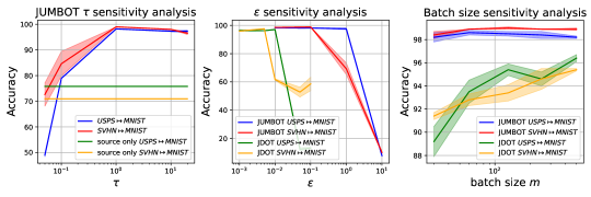
Figure 6: (Best viewed in colors) deepjdot and jumbot sensitivity analysis. We report the classification accuracy of deepjdot and jumbot on the DA tasks USPS $\mapsto$ MNIST and SVHN $\mapsto$ MNIST for several hyperparameter variations. We consider the marginal coeffifient $\tau$, the entropic coefficient $\varepsilon$ and the batch size $m$.

C.4 Overfitting

In this subsection, we discuss the training behaviour of deepjdot and our method jumbot on the DA task MNIST $\mapsto$ M-MNIST. In Figure 7, one can see that deepjdot starts overfitting from epoch 30 on each class. There are some classes which are more affected by overfitting than others. The accuracy on each class is reduced of several points. This behaviour is not shared with our method jumbot. Indeed it is more stable, it does not show any sign of overfitting and it has a higher accuracy. This shows the relevance of using our method jumbot.

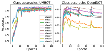
Figure 7: (Best viewed in colors) deepjdot and jumbot class accuracies along training. We report the class accuracies along training of deepjdot and jumbot on the DA task MNIST $\mapsto$ M-MNIST for optimal hyper-parameters. Each color represents a different class.

References

- Arjovsky et al. (2017) Arjovsky, M., Chintala, S., and Bottou, L. Wasserstein generative adversarial networks. In Proceedings of the 34th International Conference on Machine Learning, 2017.
- Balaji et al. (2020) Balaji, Y., Chellappa, R., and Feizi, S. Robust optimal transport with applications in generative modeling and domain adaptation. In Advances in Neural Information Processing Systems, 2020.
- Bassetti et al. (2006) Bassetti, F., Bodini, A., and Regazzini, E. On minimum kantorovich distance estimators. Statistics & Probability Letters, 76, 2006.
- Bellemare et al. (2017) Bellemare, M. G., Danihelka, I., Dabney, W., Mohamed, S., Lakshminarayanan, B., Hoyer, S., and Munos, R. The cramer distance as a solution to biased wasserstein gradients. CoRR, abs/1705.10743, 2017.
- Bernton et al. (2019) Bernton, E., Jacob, P. E., Gerber, M., and Robert, C. P. On parameter estimation with the wasserstein distance. Information and Inference: A Journal of the IMA, 8(4):657–676, 2019.
- Bertsekas (1997) Bertsekas, D. P. Nonlinear programming. Journal of the Operational Research Society, 48(3):334–334, 1997.
- Bottou (2010) Bottou, L. Large-scale machine learning with stochastic gradient descent. In in COMPSTAT, 2010.
- Cao et al. (2018) Cao, Z., Ma, L., Long, M., and Wang, J. Partial adversarial domain adaptation. In Proceedings of the European Conference on Computer Vision (ECCV), September 2018.
- Cao et al. (2019) Cao, Z., You, K., Long, M., Wang, J., and Yang, Q. Learning to transfer examples for partial domain adaptation. In The IEEE Conference on Computer Vision and Pattern Recognition (CVPR), June 2019.
- Chapel et al. (2020) Chapel, L., Alaya, M. Z., and Gasso, G. Partial optimal transport with applications on positive-unlabeled learning. In Advances in Neural Information Processing Systems, 2020.
- Chen et al. (2020) Chen, M., Zhao, S., Liu, H., and Cai, D. Adversarial-learned loss for domain adaptation. arXiv, abs/2001.01046, 2020.
- Chizat et al. (2018) Chizat, L., Peyré, G., Schmitzer, B., and Vialard, F. Scaling algorithms for unbalanced optimal transport problems. Math. Comput., 87(314):2563–2609, 2018. doi: 10.1090/mcom/3303.
- Clarke (1990) Clarke, F. H. Optimization and nonsmooth analysis. SIAM, 1990.
- Clarke (1975) Clarke, H. F. Generalized gradients and applications. Transactions of The American Mathematical Society, pp. 247–247, 1975.
- Courty et al. (2017) Courty, N., Flamary, R., Habrard, A., and Rakotomamonjy, A. Joint distribution optimal transportation for domain adaptation. In Advances in Neural Information Processing Systems, 2017.
- Courty et al. (2017) Courty, N., Flamary, R., Tuia, D., and Rakotomamonjy, A. Optimal transport for domain adaptation. IEEE Transactions on Pattern Analysis and Machine Intelligence, 2017.
- Cuturi (2013) Cuturi, M. Sinkhorn distances: Lightspeed computation of optimal transport. In Advances in Neural Information Processing Systems 26, 2013.
- Damodaran et al. (2018) Damodaran, B. B., Kellenberger, B., Flamary, R., Tuia, D., and Courty, N. DeepJDOT: Deep Joint Distribution Optimal Transport for Unsupervised Domain Adaptation. In ECCV 2018 - 15th European Conference on Computer Vision. Springer, 2018.
- Damodaran et al. (2019) Damodaran, B. B., Flamary, R., Seguy, V., and Courty, N. An Entropic Optimal Transport Loss for Learning Deep Neural Networks under Label Noise in Remote Sensing Images. In Computer Vision and Image Understanding, 2019.
- Davis et al. (2020) Davis, D., Drusvyatskiy, D., Kakade, S., and Lee, J. D. Stochastic subgradient method converges on tame functions. Foundations of computational mathematics, 20(1):119–154, 2020.
- Dhouib et al. (2020) Dhouib, S., Redko, I., Kerdoncuff, T., Emonet, R., and Sebban, M. A swiss army knife for minimax optimal transport. In International Conference on Machine Learning, pp. 2504–2513, 2020.
- Fatras et al. (2020) Fatras, K., Zine, Y., Flamary, R., Gribonval, R., and Courty, N. Learning with minibatch wasserstein : asymptotic and gradient properties. In Chiappa, S. and Calandra, R. (eds.), Proceedings of the Twenty Third International Conference on Artificial Intelligence and Statistics, volume 108 of Proceedings of Machine Learning Research, pp. 2131–2141. PMLR, 26–28 Aug 2020.
- Fatras et al. (2021) Fatras, K., Zine, Y., Majewski, S., Flamary, R., Gribonval, R., and Courty, N. Minibatch optimal transport distances; analysis and applications. CoRR, 2021.
- Feydy et al. (2019) Feydy, J., Séjourné, T., Vialard, F.-X., Amari, S.-i., Trouve, A., and Peyré, G. Interpolating between optimal transport and mmd using sinkhorn divergences. In Proceedings of Machine Learning Research, 2019.
- Figalli (2010) Figalli, A. The optimal partial transport problem. Archive for Rational Mechanics and Analysis, 195:533–560, 02 2010.
- Figalli & Gigli (2010) Figalli, A. and Gigli, N. A new transportation distance between non-negative measures, with applications to gradients flows with dirichlet boundary conditions. Journal de mathématiques pures et appliquées, 94(2):107–130, 2010.
- Flamary & Courty (2017) Flamary, R. and Courty, N. Pot python optimal transport library, 2017.
- Ganin et al. (2016) Ganin, Y., Ustinova, E., Ajakan, H., Germain, P., Larochelle, H., Laviolette, F., March, M., and Lempitsky, V. Domain-adversarial training of neural networks. Journal of Machine Learning Research, 17(59):1–35, 2016.
- Genevay et al. (2018) Genevay, A., Peyre, G., and Cuturi, M. Learning generative models with sinkhorn divergences. In Proceedings of the Twenty-First International Conference on Artificial Intelligence and Statistics, 2018.
- Genevay et al. (2019) Genevay, A., Chizat, L., Bach, F., Cuturi, M., and Peyré, G. Sample complexity of sinkhorn divergences. In Proceedings of Machine Learning Research, 2019.
- Gulrajani et al. (2017) Gulrajani, I., Ahmed, F., Arjovsky, M., Dumoulin, V., and Courville, A. C. Improved training of wasserstein gans. In Advances in Neural Information Processing Systems 30. 2017.
- Hanin (1992) Hanin, L. Kantorovich-rubinstein norm and its application in the theory of lipschitz spaces. 1992.
- Hoeffding (1963) Hoeffding, W. Probability inequalities for sums of bounded random variables. Journal of the American Statistical Association, 1963.
- Hull (1994) Hull, J. Database for handwritten text recognition research. Pattern Analysis and Machine Intelligence, IEEE Transactions on, 16, 1994. doi: 10.1109/34.291440.
- J Lee (2019) J Lee, A. U-statistics : theory and practice / a. j. lee. SERBIULA (sistema Librum 2.0), 2019.
- Jian et al. (2020) Jian, L., Yunbo, W., Dapeng, H., Ran, H., and Jiashi, F. A balanced and uncertainty-aware approach for partial domain adaptation. In European Conference on Computer Vision (ECCV), August 2020.
- Kolouri et al. (2016) Kolouri, S., Zou, Y., and Rohde, G. K. Sliced wasserstein kernels for probability distributions. In Proceedings of the IEEE Conference on Computer Vision and Pattern Recognition, 2016.
- Kuhn et al. (2019) Kuhn, D., Mohajerin Esfahani, P., Nguyen, V. A., and Shafieezadeh Abadeh, S. Wasserstein distributionally robust optimization: Theory and applications in machine learning. INFORMS TutORials in Operations Research, 2019.
- LeCun & Cortes (2010) LeCun, Y. and Cortes, C. MNIST handwritten digit database. 2010.
- Liero et al. (2017) Liero, M., Mielke, A., and Savaré, G. Optimal entropy-transport problems and a new hellinger–kantorovich distance between positive measures. Inventiones mathematicae, 211(3):969–1117, Dec 2017. ISSN 1432-1297. doi: 10.1007/s00222-017-0759-8.
- Liutkus et al. (2019) Liutkus, A., Simsekli, U., Majewski, S., Durmus, A., and Stöter, F.-R. Sliced-Wasserstein flows: Nonparametric generative modeling via optimal transport and diffusions. In Proceedings of the 36th International Conference on Machine Learning, 2019.
- Long et al. (2018) Long, M., Cao, Z., Wang, J., and Jordan, M. I. Conditional adversarial domain adaptation. In Advances in Neural Information Processing Systems, pp. 1645–1655, 2018.
- Majewski et al. (2018) Majewski, S., Miasojedow, B., and Moulines, E. Analysis of nonsmooth stochastic approximation: the differential inclusion approach. arXiv preprint arXiv:1805.01916, 2018.
- Mohajerin Esfahani & Kuhn (2018) Mohajerin Esfahani, P. and Kuhn, D. Data-driven distributionally robust optimization using the wasserstein metric: Performance guarantees and tractable reformulations. Math. Program., 171(1–2):115–166, September 2018. ISSN 0025-5610.
- Mukherjee et al. (2020) Mukherjee, D., Guha, A., Solomon, J., Sun, Y., and Yurochkin, M. Outlier-robust optimal transport. CoRR, 2020.
- Müller et al. (2019) Müller, R., Kornblith, S., and Hinton, G. E. When does label smoothing help? In Advances in Neural Information Processing Systems, 2019.
- Muzellec et al. (2020) Muzellec, B., Josse, J., Boyer, C., and Cuturi, M. Missing data imputation using optimal transport. arXiv preprint arXiv:2002.03860, 2020.
- Nath (2020) Nath, J. S. Unbalanced optimal transport using integral probability metric regularization. CoRR, 2020.
- Netzer et al. (2011) Netzer, Y., Wang, T., Coates, A., Bissacco, A., Wu, B., and Ng, A. Y. Reading digits in natural images with unsupervised feature learning. In NIPS Workshop on Deep Learning and Unsupervised Feature Learning 2011, 2011.
- Papa et al. (2015) Papa, G., Clémençon, S., and Bellet, A. Sgd algorithms based on incomplete u-statistics: Large-scale minimization of empirical risk. In Advances in Neural Information Processing Systems 28, 2015.
- Paszke et al. (2017) Paszke, A., Gross, S., Chintala, S., Chanan, G., Yang, E., DeVito, Z., Lin, Z., Desmaison, A., Antiga, L., and Lerer, A. Automatic differentiation in pytorch. 2017.
- Paty & Cuturi (2019) Paty, F.-P. and Cuturi, M. Subspace robust wasserstein distances. In International Conference on Machine Learning, pp. 5072–5081, 2019.
- Peng et al. (2017) Peng, X., Usman, B., Kaushik, N., Hoffman, J., Wang, D., and Saenko, K. Visda: The visual domain adaptation challenge. CoRR, abs/1710.06924, 2017.
- Peyré (2015) Peyré, G. Entropic approximation of wasserstein gradient flows. SIAM Journal on Imaging Sciences, 2015.
- Peyré & Cuturi (2019) Peyré, G. and Cuturi, M. Computational optimal transport. Foundations and Trends® in Machine Learning, 2019.
- Pham et al. (2020) Pham, K., Le, K., Ho, N., Pham, T., and Bui, H. On unbalanced optimal transport: An analysis of Sinkhorn algorithm. In III, H. D. and Singh, A. (eds.), Proceedings of the 37th International Conference on Machine Learning, volume 119 of Proceedings of Machine Learning Research, pp. 7673–7682. PMLR, 13–18 Jul 2020.
- Piccoli & Rossi (2014) Piccoli, B. and Rossi, F. On properties of the generalized wasserstein distance, 2014.
- Schmitzer & Wirth (2017) Schmitzer, B. and Wirth, B. A framework for wasserstein-1-type metrics. ArXiv, abs/1701.01945, 2017.
- Séjourné et al. (2019) Séjourné, T., Feydy, J., Vialard, F.-X., Trouvé, A., and Peyré, G. Sinkhorn divergences for unbalanced optimal transport. arXiv preprint arXiv:1910.12958, 2019.
- Shen et al. (2018) Shen, J., Qu, Y., Zhang, W., and Yu, Y. Wasserstein distance guided representation learning for domain adaptation. In Proceedings of the AAAI Conference on Artificial Intelligence, volume 32, 2018.
- Sommerfeld et al. (2019) Sommerfeld, M., Schrieber, J., Zemel, Y., and Munk, A. Optimal transport: Fast probabilistic approximation with exact solvers. Journal of Machine Learning Research, 2019.
- Venkateswara et al. (2017) Venkateswara, H., Eusebio, J., Chakraborty, S., and Panchanathan, S. Deep hashing network for unsupervised domain adaptation. In (IEEE) Conference on Computer Vision and Pattern Recognition (CVPR), 2017.