Thermodynamic topology optimization including plasticity

Miriam Kick, Philipp Junker
Leibniz University Hannover, Institute of Continuum Mechanics, Hannover, Germany
Corresponding author:
Philipp Junker, ✉ junker@ikm.uni-hannover.de

Abstract

Topology optimization is an important basis for the design of components. Here, the optimal structure is found within a design space subject to boundary conditions as well as the material law. Additionally, the specific material law has a strong impact on the final design. Even more: a, for instance, linear-elastically structure is not optimal if plastic deformation will be induced by the loads. Hence, a physically correct and resource-efficient inclusion of plasticity modeling is needed. In this contribution, we present an extension of the thermodynamic topology optimization that accounts for the non-linear material behavior due to the evolution of plastic strains. For this purpose, we develop a novel surrogate plasticity model that allows to compute the correct plastic strain tensor corresponding to the current structure design. We show the agreement of the model with the classic plasticity model without dissipation and that the interaction of the topology optimization with plastic material behavior results in structural changes.

1 Introduction

Engineers are always looking for structures that meet the specific requirements in an optimal way. One possibility for finding these structures is provided by optimization schemes which are classified as follows: i) improving the principal idea, ii) modifying the material, iii) thickness dimensioning, iv) optimization of shape and v) optimization of topology [29, 16]. Herein, the optimization scheme that demands the minimum amount of restrictions is given by topology optimization. The consideration of the real materials properties offers additional potential for the optimal design of components. Therefore, it is important to account for the physical material behavior even during the process of topology optimization.

There are various variants of topology optimization available as, e. g., the optimization for temperature evolution, noise reduction, dynamic response, or structural stiffness. All of these approaches have in common that the related physical balance laws, in most cases the balance of linear momentum, are solved along with a mathematical optimization problem which is given in terms of an objective function. The most common objective is the minimization of compliance, i. e. the maximization of stiffness according to a target structure volume [30]. Therefore, topology optimization determines the position and arrangement of material within a given design space and boundary conditions such that the objective function is minimized. The topology of a structure can be parameterized via different approaches during the specific numerical investigation. For the numerical solution of the physical balance law, e. g., the balance of linear momentum, usually the finite element method (FEM) is employed. Consequently, the finite elements introduce a discretization of the design space, and it is thus most common to assign a density value for each discrete subvolume, i. e. for each finite element. For this assignment, a variety of different numerical schemes has been developed among which the probably most popular is given by “Solid Material with Penalization” (SIMP) proposed by Bendsøe and Sigmund in [5, 6]. The fundamental idea of SIMP is the introduction of a non-linear interpolation function between void and full material such that a black and white design is aspired due to the inherent non-convex total potential. Further popular developments are overviewed in [30, 12].

In a series of papers, we aimed at contributing to the problem of topology optimization: by using thermodynamic extremal principles, evolutionary access to the problem of topology optimization has been presented for which we referred our method to as thermodynamic topology optimization (TTO). It routes back to [22] while further important developments have been presented for the numerical treatment in [17] and for hyperelastic material in [21]. This topology optimization makes use of an extended Hamilton principle which is well-known in the context of material modeling, cf. [20]. Therefore, the extended Hamilton functional is formulated and its stationarity conditions serve as update procedure for the evolution of the topology. In this manner, no classical optimization problem is formulated. Since the free energy function is part of the extended Hamilton functional, the result is very similar to classical schemes for topology optimization [18]. The manipulation of topology is managed by the density as state variable which is defined for each discretized area. One advantage of this thermodynamic topology optimization is that no further optimization algorithm is needed. In contrast, the relative density is described by a transient partial differential equation (PDE) in which the local free energy density serves as source term. Consequently, the material optimization problem is converted to an evolutionary problem. The field equation for the topology results from the stationary condition of the extended Hamilton functional. Additionally, evaluation of the functional results in the field equations for displacement and internal (state) variable which accounts for the (local) microstructure of the material. From this follows that the extended Hamilton functional according to topology optimization also features to take any physically dissipative material behavior into account.

In context of accounting for a real material behavior during the optimization, the plastic material behavior plays a major role which requires a thermodynamically and mathematically rigorous treatment due to its complexity. Direct access of plastic material behavior within topology optimization might be given by using classical plasticity models with the characteristic stress/strain diagram resulting in a hysteresis curve in cyclic loading. Several successful examples are provided in the literature: a first approach to account for a classical elasto-plastic material model within an adaptive material topology optimization was proposed by Maute et al. [27]. Approaches to determine plasticity by homogenization strategies are also possible, cf. [36]. This is particularly interesting for plastic parts of composites [31]. Furthermore, topology optimization based on finite strains can be considered for plasticity [33]. Nakshatrala and Tortorelli [28] optimize dynamically loaded structures while accounting for plastic material behavior. A different option was proposed by the consideration of damage, cf. [25, 1]. For all such non-linear stress/strain relations, the optimization routine usually demands an additional algorithm for convergence. Here, one prominent possibility is provided by the “method of moving asymptotes” (MMA).

Unfortunately, the strategy of considering physical material models usually renders such optimization rather time-consuming: due to the local path-dependence, the physical loading process needs to be discretized with several time steps each of which demands the solution of the physical finite element problem. The nested finite element simulations for the physical process and the topology optimization problem demand a remarkably higher amount of computation time. To compensate this drawback, several strategies can be found which aim to directly include plasticity into the optimization process: one approach is to couple an elastic model with local stress constraint as mentioned e. g. by [13, 14, 8, 26]. Another idea by Amir [2] is to define a single global stress constraint within the formulation of optimization problem to bypass the local calculation for each material point. Bruns et al. [9] propose to constrain the load-displacement by limit points in case of damage. Another way is to account for the nonlinear material behavior on a second, microscopic scale by developing a new model reduction technique which is proposed by Fritzen et al. [15] and extended by Xia et al. [35]. A special characteristic of this approach is the use of an evolutionary optimization method on the macroscopic scale. Furthermore, surrogate models have been developed which avoid the need of solving physical finite element problems. Zhao et al. [38, 37], for instance, developed a surrogate model as a fictitious non-linear elastic material model which asymptotically approximates a perfect elasto-plastic behavior. They accounted for the von Mises criterion in [38] and also developed an approach valid for the Drucker-Prager criterion in [37]. Due to the absent path-dependence, the computation of the sensitivity is straight forward and only one finite element analysis needs to be computed for each iteration step. Therefore, this approach has a remarkable disadvantage that the resulting stress/strain curve matches the similar classical elasto-plastic curve even at a material point level only at the limit points. Furthermore, there is no possibility to compute the plastic strain tensor which serve as thermodynamic state variable.

Hence, a topology optimization method accounting for plastic material behavior in a resource-efficient manner is missing. In this contribution, we aim at expanding the thermodynamic topology optimization such that it can be applied to elasto-plastic materials with a novel 3D surrogate material model. Therefore, the surrogate model is based on a classical plastic material model whereby the mentioned disadvantages of non-linearity and path-dependence should be prevented by modifications resulting from the nature of optimization: we determine topology optimization results for the (maximal) external loading; unloading and cyclic load curves are not investigated here. During an evolutionary optimization process the topology and the resulting structural stiffness evolve, respectively. Differently stiff structures loaded with the same external loading result in different displacement fields. Therefore, the displacement field also evolves during the optimization process. For instance, high strains might be present in the beginning of the optimization process with associated high plastic strains. However, the evolution of local stiffness results in reduced strains and consequently reduced plastic strains. Since this “unloading” process does not correspond to the physical evolution of plastic strains but occurs due to the evolution of the topology optimization we denote for this as “virtual unloading”. For a classical plasticity model, the virtual unloading evokes dissipation which results in the typical hysteresis curve. However, we are interested in a material model that computes the plastic strains for each displacement state as it results from physical loading. Therefore, the surrogate model must reflect the physically correct stress/strain curve during loading, i. e. without any effects due to virtual unloading – the unloading process must not correspond to the physical evolution of plastic strains. In the case of virtual unloading the loading branch in the stress/strain curve needs to be followed backwards. To this end, we propose a hysteresis-free behavior for the surrogate model by suppressing the dissipative character. Finally, this results in the following benefits of the surrogate model: i) the surrogate model matches the results of plastic material models at the material point level, ii) the physical state variable can be measured in terms of the plastic strain tensor and iii) the total number of finite element simulations can be reduced while the material behavior is still physically accurate. Consequently, our surrogate model in terms of the thermodynamic topology optimization allows finding optimal structures if plastic material behavior occurs.

The paper is structured as follows: first, we recall the basics of the thermodynamic topology optimization by use of Hamilton’s principle and complement our previous approaches by the inclusion of plasticity. To this end, we develop a surrogate material model for our topology optimization approach that accounts for plasticity without consideration of dissipation-related hysteresis effects. Afterwards we present a suitable strategy for numerical implementation. Finally, the functionality of the proposed approach is tested and analyzed by means of computing topology optimizations for several boundary value problems.

2 Surrogate model for plasticity developed in thermodynamic topology optimization

The thermodynamic topology optimization is based on Hamilton’s principle which is usually a variational strategy for material modeling [20]. Assuming stationary of an extended Hamilton functional follows the thermodynamic and physical laws and yields field equations for all state variables i. e. displacements, temperature and internal variables. Expanding the functional for topology optimization provides the benefit that the optimization problem can be tackled by a system of partial differential equations. Consequently, the mathematical optimization problem is converted into an evolutionary problem. At the same time, the stationarity of the extended Hamilton functional comprises the evolution of microstructural material behavior which affects the evolution of topology. Furthermore, constraints on the topology design as well as on the material behavior can be considered easily by taking use of Lagrange or Karush Kuhn Tucker parameters. It is worth mentioning that no classical optimization problem is solved in thermodynamic topology optimization. In contrast, the stationarity condition of the Hamilton functional with respect to the density variable serves as update scheme for the topology.

We use the following notation for tensor operations: the single contraction is noted as “$\cdot$” reading $\boldsymbol{a}\cdot\boldsymbol{b}=c\Leftrightarrow a_{i}b_{i}=c$ when applied to two vectors $\boldsymbol{a}$ and $\boldsymbol{b}$, while it results in $\boldsymbol{A}\cdot\boldsymbol{b}=\boldsymbol{c}\Leftrightarrow A_{ij}b_{j}=c_{i}$ when applied to a vector and a second-order tensor $\boldsymbol{A}$. Moreover, the double contraction is denoted as “$:$”. It results in $\boldsymbol{A}:\boldsymbol{B}=c\Leftrightarrow A_{ij}B_{ij}=c$ when applied to two second-order tensors while it results in $\mathbb{A}:\boldsymbol{B}=\boldsymbol{C}\Leftrightarrow\mathbb{A}_{ijkl}B_{kl}=C_{ij}$ when applied to a fourth-order tensor $\mathbb{A}$ and a second-order tensor. Finally, the tensor product, i. e. the dyadic product, is noted as “$\otimes$” and reads $\boldsymbol{a}\otimes\boldsymbol{b}=\boldsymbol{C}\Leftrightarrow a_{i}b_{j}=C_{ij}$ when applied to two vectors and $\boldsymbol{A}\otimes\boldsymbol{B}=\mathbb{C}\Leftrightarrow A_{ij}B_{kl}=\mathbb{C}_{ijkl}$ when applied to two second-order tensors.

In this contribution, the approach of topology optimization does not account for dynamic effects and therefore, we consider quasi-static loading. Here, the extended Hamilton functional [20] for a quasi-static and isothermal case reads

(1) $$\bar{\mathcal{H}}=\bar{\mathcal{H}}\left[\boldsymbol{u},\boldsymbol{y}\right]:=\mathcal{G}\left[\boldsymbol{u},\boldsymbol{y}\right]+\mathcal{D}\left[\boldsymbol{\alpha}\right]$$

and sums the Gibbs energy $\mathcal{G}$ and the dissipation-related work $\mathcal{D}$. This functional depends on the displacements $\boldsymbol{u}$ and the state variable $\boldsymbol{y}=\{\boldsymbol{\alpha},\chi\}$. The state variable is decomposed into the vectorial quantity $\boldsymbol{\alpha}$ collecting all internal variables which describe the physical material behavior in terms of the microstructural state. In our case of an elasto-plastic material, we thus chose $\boldsymbol{\alpha}=\boldsymbol{\varepsilon}^{\mathrm{p}}$ where $\boldsymbol{\varepsilon}^{\mathrm{p}}$ denotes the plastic part of the strain and $\boldsymbol{\varepsilon}^{\mathrm{e}}$ the elastic part, i. e. $\boldsymbol{\varepsilon}=\boldsymbol{\varepsilon}^{\mathrm{e}}+\boldsymbol{\varepsilon}^{\mathrm{p}}$. The quantity $\chi$ denotes the density variable for defining the topology. Here, the density variable $\chi\in[\chi_{\mathrm{min}},1]$ with $\chi_{\mathrm{min}}>0$ represents void “white” material for $\chi=\chi_{\mathrm{min}}$, the full “black” material for $\chi=1$, and a mixed “gray” phase for $\chi\in]\chi_{\mathrm{min}},1[$. The relative density is then modeled via the SIMP approach [6] by the interpolation function

(2) $$\rho(\chi)=\chi^{3}\,,$$

for instance. Other approaches are also possible, see [21] where a sigmoid function has been used.

According to Hamilton’s principle the stationary condition of the functional is provided as

(3) $$\bar{\mathcal{H}}=\bar{\mathcal{H}}[\boldsymbol{u},\boldsymbol{\varepsilon}^{\mathrm{p}},\chi]:=\mathcal{G}\left[\boldsymbol{u},\boldsymbol{\varepsilon}^{\mathrm{p}},\chi\right]+\mathcal{D}\left[\boldsymbol{\varepsilon}^{\mathrm{p}}\right]\rightarrow\underset{\boldsymbol{u},\boldsymbol{\varepsilon}^{\mathrm{p}},\chi}{\text{stat}}\ .$$

Therein, $\mathcal{G}$ is defined as difference between the energy stored in the body with volume $\Omega$ and the work due to external forces. It hence reads

(4) $$\mathcal{G}\left[\boldsymbol{u},\boldsymbol{\varepsilon}^{\mathrm{p}},\chi\right]:=\int_{\Omega}\Psi(\boldsymbol{\varepsilon}^{\mathrm{e}},\chi)\ \mathrm{d}V-\int_{\Omega}\boldsymbol{b}^{\star}\cdot\boldsymbol{u}\ \mathrm{d}V-\int_{\Gamma_{\sigma}}\boldsymbol{t}^{\star}\cdot\boldsymbol{u}\ \mathrm{d}A$$

with the Helmholtz free energy $\Psi$, the body forces $\boldsymbol{b}^{\star}$ and the traction vector $\boldsymbol{t}^{\star}$. The boundary conditions are defined as Dirichlet conditions for $\boldsymbol{u}^{\star}$ on $\Gamma_{u}$ and as Neumann conditions for $\boldsymbol{t}^{\star}$ on $\Gamma_{\sigma}$. Hence, the complete boundary $\partial\Omega$ of the body is given by $\partial\Omega=\Gamma_{u}\cup\Gamma_{\sigma}$ and $\Gamma_{u}\cap\Gamma_{\sigma}=\varnothing$. Furthermore, the dissipation-related work is defined by

(5) $$\mathcal{D}:=\int_{\Omega}\boldsymbol{p}^{\mathrm{diss}}:\boldsymbol{\varepsilon}^{\mathrm{p}}\ \mathrm{d}V$$

with the non-conservative force $\boldsymbol{p}^{\mathrm{diss}}$ which can be derived from the dissipation function $\Delta^{\mathrm{diss}}$ by

(6) $$\boldsymbol{p}^{\mathrm{diss}}:=\frac{\partial\Delta^{\mathrm{diss}}}{\partial\dot{\boldsymbol{\varepsilon}}^{\mathrm{p}}}\ .$$

More details on the thermodynamic basis are provided in [20]. According to [21], the physically motivated Hamilton functional $\bar{\mathcal{H}}$ can be extended for thermodynamic topology optimization by adding

(7) $$\mathcal{H}\left[\boldsymbol{u},\boldsymbol{\varepsilon}^{\mathrm{p}},\chi\right]:=\bar{\mathcal{H}}\left[\boldsymbol{u},\boldsymbol{\varepsilon}^{\mathrm{p}},\chi\right]-\mathcal{R}\left[\chi\right]+\mathcal{C}\left[\boldsymbol{\varepsilon}^{\mathrm{p}},\chi\right]\ .$$

where additional constraints are included in $\mathcal{C}$ and the rearrangement of topology is accounted for by the functional $\mathcal{R}$, defined as

(8) $$\mathcal{R}\left[\chi\right]:=\mathcal{D}_{\chi}\left[\chi\right]+\mathcal{F}\left[\chi\right]\ .$$

Here, the flux term

(9) $$\mathcal{F}\left[\chi\right]:=\int_{\Omega}\frac{1}{2}\,\beta\,\left\lVert\nabla\chi\right\rVert^{2}\ \mathrm{d}V$$

accounts for the convective rearrangement with the regularization parameter $\beta>0$. It thus serves as gradient penalization for the density variable and also controls the members size via the parameter $\beta$. Additionally, the source term

(10) $$\mathcal{D}_{\chi}\left[\chi\right]:=\int_{\Omega}p^{\mathrm{diss}}_{\chi}\,\chi\ \mathrm{d}V$$

accounts for local rearrangement. Analogously to (6), the non-conservative term for local rearrangement is assumed to be derivable from an associated dissipation function according to

(11) $$p^{\mathrm{diss}}_{\chi}:=\frac{\partial\Delta^{\mathrm{diss}}_{\chi}}{\partial\dot{\chi}}\ .$$

For the dissipation function, we follow [17] and chose

(12) $$\Delta^{\mathrm{diss}}_{\chi}=\frac{1}{2}\,\eta\,\dot{\chi}^{2}\ .$$

The viscosity parameter $\eta>0$ controls the velocity of evolution of topology. In this manner, the Hamilton functional (7) is able to couple microstructure evolution and topology optimization. We propose that an optimal structure can be found if this functional becomes stationary.

The stationary condition with respect to all variables

(13) $$\delta\mathcal{H}=\delta_{\boldsymbol{u}}\mathcal{H}+\delta_{\boldsymbol{\varepsilon}^{\mathrm{p}}}\mathcal{H}+\delta_{\chi}\mathcal{H}=0\qquad\forall\;\delta_{\boldsymbol{u}},\delta_{\boldsymbol{\varepsilon}^{\mathrm{p}}},\delta_{\chi}$$

yields the following system of governing equations

(14) $$\left\{\begin{array}[]{@{}l@{\quad}l@{}}\displaystyle\delta_{\boldsymbol{u}}\mathcal{H}=0=\int_{\Omega}\frac{\partial\Psi}{\partial\boldsymbol{\varepsilon}}:\delta\boldsymbol{\varepsilon}\ \mathrm{d}V-\int_{\Omega}\boldsymbol{b}^{\star}\cdot\delta\boldsymbol{u}\ \mathrm{d}V-\int_{\Gamma_{\sigma}}\boldsymbol{t}^{\star}\cdot\delta\boldsymbol{u}\ \mathrm{d}A&\forall\;\delta\boldsymbol{u}\\[11.38109pt] \displaystyle\delta_{\boldsymbol{\varepsilon}^{\mathrm{p}}}\mathcal{H}=0=\int_{\Omega}\frac{\partial\Psi}{\partial\boldsymbol{\varepsilon}^{\mathrm{p}}}:\delta\boldsymbol{\varepsilon}^{\mathrm{p}}\ \mathrm{d}V+\int_{\Omega}\frac{\partial\Delta^{\mathrm{diss}}}{\partial\dot{\boldsymbol{\varepsilon}}^{\mathrm{p}}}:\delta\boldsymbol{\varepsilon}^{\mathrm{p}}\ \mathrm{d}V+\delta_{\boldsymbol{\varepsilon}^{\mathrm{p}}}\,\mathcal{C}&\forall\;\delta\boldsymbol{\varepsilon}^{\mathrm{p}}\\[11.38109pt] \displaystyle\delta_{\chi}\mathcal{H}=0=\int_{\Omega}\frac{\partial\Psi}{\partial\chi}\ \delta\chi\ \mathrm{d}V-\int_{\Omega}\eta\,\dot{\chi}\,\delta\chi\ \mathrm{d}V-\int_{\Omega}\beta\ \nabla\chi\cdot\nabla\delta\chi\ \mathrm{d}V+\delta_{\chi}\,\mathcal{C}&\forall\;\delta\chi\end{array}\right.$$

where each equation belongs to one of the independent system variables, cf. also [21] for a general microstructure consideration in case of finite deformations. Here, the standard notation $\delta\boldsymbol{\varepsilon}:=\mathrm{sym}(\nabla\otimes\delta\boldsymbol{u})$ is used. The first condition is identified as the weak form of the balance of the linear momentum where the stress is given by $\boldsymbol{\sigma}=\partial\Psi/\partial\boldsymbol{\varepsilon}$. The second condition constitutes as governing equation for the plastic strains $\boldsymbol{\varepsilon}^{\mathrm{p}}$ and the last equation is the field equation for topology optimization.

2.1 Specification of the energetic quantities and the constraints

The system of governing equations (14) establishes the general framework for the optimization process. However, by specification of the free energy density $\Psi$, the dissipation function $\Delta^{\mathrm{diss}}$, and the constraint functional $\mathcal{C}$ the characteristics of the surrogate material model for plasticity and the density variable are defined.

For the free energy, we follow the classical approach of elasto-plastic materials and combine it with the relative density $\rho(\chi)$ in (2). This gives

(15) $$\Psi(\boldsymbol{\varepsilon}^{\mathrm{e}},\chi)=\rho(\chi)\,\Psi_{0}:=\frac{1}{2}\,(\boldsymbol{\varepsilon}-\boldsymbol{\varepsilon}^{\mathrm{p}}):\chi^{3}\,\mathbb{E}_{0}:(\boldsymbol{\varepsilon}-\boldsymbol{\varepsilon}^{\mathrm{p}})$$

where the stiffness tensor of the full material is given by $\mathbb{E}_{0}$ and the energy of the virtually full material is given by

(16) $$\Psi_{0}:=\frac{1}{2}\,(\boldsymbol{\varepsilon}-\boldsymbol{\varepsilon}^{\mathrm{p}}):\mathbb{E}_{0}:(\boldsymbol{\varepsilon}-\boldsymbol{\varepsilon}^{\mathrm{p}})\,.$$

Consequently, we obtain for the stresses

(17) $$\boldsymbol{\sigma}=\frac{\partial\Psi}{\partial\boldsymbol{\varepsilon}}=\chi^{3}\,\mathbb{E}_{0}:(\boldsymbol{\varepsilon}-\boldsymbol{\varepsilon}^{\mathrm{p}})\ .$$

The derivative of $\Psi$ with respect to $\boldsymbol{\varepsilon}^{\mathrm{p}}$ thus yields

(18) $$\frac{\partial\Psi}{\partial\boldsymbol{\varepsilon}^{\mathrm{p}}}=-\boldsymbol{\sigma}$$

and the derivative of $\Psi$ with respect to $\chi$ yields

(19) $$p:=-\frac{\partial\Psi}{\partial\chi}=-3\,\chi^{2}\,\Psi_{0}$$

as driving force or sensitivity for the topology optimization, respectively. The driving force $p$ is non-zero for all conditions with $\Psi_{0}\not=0$ since $\chi>\chi_{\text{min}}$. Furthermore, the evolution of plastic strains influences $\Psi_{0}$ and, in turn, the driving force $p$ and thus the update condition for optimization, cf. (14)₃.

The following equations formulate the surrogate material model for the evolution of plastic strains in the context of thermodynamic topology optimization regarding three assumptions. The first one concerns the dissipation function. In a classical elasto-plastic material model, the dissipation function is defined as

(20) $$\Delta^{\mathrm{diss}}=r\,\left\lVert\dot{\boldsymbol{\varepsilon}}^{\mathrm{p}}\right\rVert$$

with the yield limit $r$. This approach yields a rate-independent formulation. Details on such an approach can be found, e. g., in [19, 20]. However, this physically motivated choice would contradict our intention to prevent the path-dependence and the related dissipative material behavior. Therefore, we assume that the dissipation-free evolution of plastic strains within the surrogate model is acquired by postulating a vanishing dissipation function, i. e.

(21) $$\Delta^{\mathrm{diss}}=0\,.$$

The second assumption is that the yield condition is included by demanding

(22) $$\left\lVert\boldsymbol{\sigma}^{\mathrm{dev}}\right\rVert=r$$

during plastic evolution where the stress deviator $\boldsymbol{\sigma}^{\mathrm{dev}}=\boldsymbol{\sigma}-1/3\ \mathrm{tr}\,\boldsymbol{\sigma}\boldsymbol{I}$ is computed by

(23) $$\boldsymbol{\sigma}^{\mathrm{dev}}=\mathbb{P}:\boldsymbol{\sigma}$$

with the projection tensor $\mathbb{P}$. The threshold value $r$ will be defined phenomonologically and needs to be combined with the relative density $\rho\left(\chi\right)$ according to [13] for physical consistency. Therefore, ideal plasticity is determined by a constant material parameter, e. g. the yield stresses $\sigma^{\mathrm{Y}}$, which yields

(24) $$r=\chi^{3}\,\sigma^{\mathrm{Y}}\,.$$

Hardening can be included by choosing a non-constant $r=r(\left\lVert\boldsymbol{\varepsilon}^{\mathrm{p}}\right\rVert)$. To this end, we propose linear hardening by defining

(25) $$r=r(\left\lVert\boldsymbol{\varepsilon}^{\mathrm{p}}\right\rVert)=\chi^{3}\left(\sigma^{\mathrm{Y}}+h\,\left\lVert\boldsymbol{\varepsilon}^{\mathrm{p}}\right\rVert\right)$$

with the slope of hardening curve $h$ and exponential hardening according to [23] by

(26) $$r=r(\left\lVert\boldsymbol{\varepsilon}^{\mathrm{p}}\right\rVert)=\chi^{3}\left(\sigma^{\mathrm{Y}}+h_{1}\,\left\lVert\boldsymbol{\varepsilon}^{\mathrm{p}}\right\rVert+\frac{1}{\kappa}\,\left(h_{1}-h_{0}\right)\left(e^{-\kappa\,\left\lVert\boldsymbol{\varepsilon}^{\mathrm{p}}\right\rVert}-1\right)\right)\,.$$

Here, $h_{0}$ denotes the initial and $h_{1}$ the end slope of the hardening curve and $\kappa$ controls the transition from $h_{0}$ to $h_{1}$. Since our approach is equivalent for different definitions of $r$, we always use the general notation $r$ as yield criterion in the following.

The third assumption is that the plastic strains are volume-preserving, i. e.

(27) $$\mathrm{tr}\,\boldsymbol{\varepsilon}^{\mathrm{p}}=0\,\Leftrightarrow\,\boldsymbol{I}:\boldsymbol{\varepsilon}^{\mathrm{p}}=0\,.$$

This assumption combined with the above equations and definitions yield in a non-linear algebraic equation for the determination of the plastic strains in the following Sec. 2.2. Regarding the volume-preservation condition, this equation would be ill-posed due to a projection onto the deviator subspace. Hence, no unique solution exists and a special numerical solution would be needed for the solution. However, we found to account for the volume-preservation of the plastic strains in a more efficient way, so that the resulting non-linear algebraic equation is well-posed: we make use of the hydrostatic stress by

(28) $$\mathrm{tr}\,\boldsymbol{\sigma}=\boldsymbol{I}:\boldsymbol{\sigma}=\boldsymbol{I}:\chi^{3}\,\mathbb{E}_{0}:\left(\boldsymbol{\varepsilon}-\boldsymbol{\varepsilon}^{\mathrm{p}}\right)$$

and apply the volume-preserving (27) so that with $\boldsymbol{I}:\chi^{3}\,\mathbb{E}_{0}:\boldsymbol{\varepsilon}^{\mathrm{p}}=0$ the constraint reads

(29) $$\boldsymbol{I}:\boldsymbol{\sigma}=\boldsymbol{I}:\chi^{3}\,\mathbb{E}_{0}:\boldsymbol{\varepsilon}\,.$$

The limitation of the stress norm by the yield threshold and the volume preservation are included through the constraint functional by using the Lagrange parameters $\lambda_{\mathrm{\sigma}}$ and $\lambda_{\mathrm{V}}$, respectively.

It remains to identify the constraints for the density variable $\chi$ to finally formulate the constraint functional $\mathcal{C}$. The first constraint is given by the interval in which $\chi$ is defined: values of $\chi$ that are negative are not reasonable; same limitation holds true for values of $\chi$ that are larger than one. Consequently, we demand $\chi\in[\chi_{\mathrm{min}},1]$ where the lower bound is set to a small value $1\gg\chi_{\mathrm{min}}>0$ due to numerical reasons. These bounds are taken into account by use of a Karush Kuhn Tucker parameter $\gamma$. Furthermore, the volume of the topology relative to the total design volume is prescribed by the parameter $v_{0}$. Consequently, it has to hold

(30) $$\int_{\Omega}\chi\ \mathrm{d}V=v_{0}\,\Omega$$

which is included to the constraint functional by use of a Lagrange parameter $\lambda_{\mathrm{\chi}}$.

Combining these four constraints, i. e. norm of the stress deviator being equivalent to the yield threshold $r$, volume preservation of the plastic strains $\boldsymbol{\varepsilon}^{\mathrm{p}}$, bounded interval for $\chi$, and control of the total relative structure volume $v_{0}$, we finally arrive at

(31) $$\mathcal{C}:=\lambda_{\mathrm{\sigma}}\int_{\Omega}\left(\left\lVert\boldsymbol{\sigma}^{\mathrm{dev}}\right\rVert-r\right)\ \mathrm{d}V+\lambda_{\mathrm{V}}\int_{\Omega}\left(\boldsymbol{I}:\boldsymbol{\sigma}-\boldsymbol{I}:\chi^{3}\,\mathbb{E}_{0}:\boldsymbol{\varepsilon}\right)\ \mathrm{d}V\\ +\int_{\Omega}\gamma\,\chi\ \mathrm{d}V+\lambda_{\mathrm{\chi}}\left(\int_{\Omega}\chi\ \mathrm{d}V-v_{0}\,\Omega\right)\ .$$

2.2 The stationarity condition with respect to the plastic strains

It remains to appropriately analyze the stationarity condition of the Hamilton functional with respect to the plastic strains. This conditions enables us to compute the plastic strains which, in combination with the total strain, specify the stress state. To this end, we use the specifications for a vanishing dissipation function $\Delta^{\mathrm{diss}}$ and the constraint functional (31) to evaluate (14)₂ as

$$\int_{\Omega}\left(-\boldsymbol{\sigma}+\lambda_{\mathrm{\sigma}}\left[\frac{\partial\left\lVert\boldsymbol{\sigma}^{\mathrm{dev}}\right\rVert}{\partial\boldsymbol{\varepsilon}^{\mathrm{p}}}-\frac{\partial r}{\partial\boldsymbol{\varepsilon}^{\mathrm{p}}}\right]-\lambda_{\mathrm{V}}\,\boldsymbol{I}:\chi^{3}\,\mathbb{E}_{0}\right):\delta\boldsymbol{\varepsilon}^{\mathrm{p}}\ \mathrm{d}V=0\qquad\forall\;\delta\boldsymbol{\varepsilon}^{\mathrm{p}}$$

$$\Rightarrow\quad-\boldsymbol{\sigma}+\lambda_{\mathrm{\sigma}}\left[\frac{\partial\left\lVert\boldsymbol{\sigma}^{\mathrm{dev}}\right\rVert}{\partial\boldsymbol{\varepsilon}^{\mathrm{p}}}-\frac{\partial r}{\partial\boldsymbol{\varepsilon}^{\mathrm{p}}}\right]-\lambda_{\mathrm{V}}\,\boldsymbol{I}:\chi^{3}\,\mathbb{E}_{0}$$

(32) $$=-\boldsymbol{\sigma}-\lambda_{\mathrm{\sigma}}\left[\frac{\boldsymbol{\sigma}^{\mathrm{dev}}}{\left\lVert\boldsymbol{\sigma}^{\mathrm{dev}}\right\rVert}:\mathbb{P}:\chi^{3}\,\mathbb{E}_{0}+\frac{\partial r}{\partial\boldsymbol{\varepsilon}^{\mathrm{p}}}\right]-\lambda_{\mathrm{V}}\,\boldsymbol{I}:\chi^{3}\,\mathbb{E}_{0}=0\,.$$

Solving (2.2) for the plastic strains constitutes our surrogate model for the plastic material behavior. A detailed derivation of the Lagrange multipliers is deferred to App. A. There, we show that the governing equation for the plastic strains is given as

$$\boldsymbol{s} := -\boldsymbol{\sigma}+\frac{r^{3}}{\displaystyle\boldsymbol{\sigma}^{\mathrm{dev}}:\chi^{3}\,\mathbb{E}_{0}:\boldsymbol{\sigma}^{\mathrm{dev}}+\frac{\partial r}{\partial\boldsymbol{\varepsilon}^{\mathrm{p}}}:\boldsymbol{\sigma}^{\mathrm{dev}}\,r}\,\left[\frac{\boldsymbol{\sigma}^{\mathrm{dev}}:\chi^{3}\,\mathbb{E}_{0}}{r}+\frac{\partial r}{\partial\boldsymbol{\varepsilon}^{\mathrm{p}}}\right]$$

$$+\frac{\boldsymbol{I}:\chi^{3}\,\mathbb{E}_{0}:\boldsymbol{\varepsilon}}{\boldsymbol{I}:\mathbb{E}_{0}:\boldsymbol{I}}\,\boldsymbol{I}:\mathbb{E}_{0}=\boldsymbol{0}$$

which is a non-linear algebraic equation. The derivative of the yield criterion $r$ is defined as

(34) $$\frac{\partial r}{\partial\boldsymbol{\varepsilon}^{\mathrm{p}}}=\left\{\begin{array}[]{@{}l@{\quad}l@{}}\displaystyle\boldsymbol{0}&\text{ideal plasticity}\\ \displaystyle\frac{\partial r\left(\left\lVert\boldsymbol{\varepsilon}^{\mathrm{p}}\right\rVert\right)}{\partial\boldsymbol{\varepsilon}^{\mathrm{p}}}=\frac{\partial r\left(\left\lVert\boldsymbol{\varepsilon}^{\mathrm{p}}\right\rVert\right)}{\partial\left\lVert\boldsymbol{\varepsilon}^{\mathrm{p}}\right\rVert}\,\frac{\partial\left\lVert\boldsymbol{\varepsilon}^{\mathrm{p}}\right\rVert}{\partial\boldsymbol{\varepsilon}^{\mathrm{p}}}=r^{\prime}\,\frac{\boldsymbol{\varepsilon}^{\mathrm{p}}}{\left\lVert\boldsymbol{\varepsilon}^{\mathrm{p}}\right\rVert}&\text{hardening}\end{array}\right.$$

where the term $r^{\prime}$ for the defined types of hardenings reads

(35) $$r^{\prime}=\left\{\begin{array}[]{@{}l@{\quad}l@{}}\displaystyle h&\text{linear hardening}\\ \displaystyle h_{1}-\left(h_{1}-h_{0}\right)\,e^{-\kappa\,\left\lVert\boldsymbol{\varepsilon}^{\mathrm{p}}\right\rVert}&\text{exponential hardening}\end{array}\right.\,.$$

In case of ideal plasticity with $r=\text{constant}$ and the derivative from (34), we can reduce (2.2) to

(36) $$\boldsymbol{s}^{\mathrm{ip}}:=-\boldsymbol{\sigma}+\frac{r^{2}}{\boldsymbol{\sigma}^{\mathrm{dev}}:\mathbb{E}_{0}:\boldsymbol{\sigma}^{\mathrm{dev}}}\,\boldsymbol{\sigma}^{\mathrm{dev}}:\mathbb{E}_{0}+\frac{\boldsymbol{I}:\chi^{3}\,\mathbb{E}_{0}:\boldsymbol{\varepsilon}}{\boldsymbol{I}:\mathbb{E}_{0}:\boldsymbol{I}}\,\boldsymbol{I}:\mathbb{E}_{0}=\boldsymbol{0}\,.$$

Remark: it is worth mentioning that we do not receive a differential equation for the internal variable as it is usually the case. This routes back to assuming a dissipation-free evolution of the plastic strains which, in turn, are determined by energy minimization.

Components of the plastic strain tensor only evolve to compensate high stresses which are greater than the yield stress $\sigma^{\mathrm{Y}}$. Therefore, it is mandatory to identify a suitable criterion for distinguishing whether an elastic or plastic material behavior is present. Since the purpose of the modified surrogate plasticity model is to display the same material behavior for loading like a classical material model for elasto-plasticity, we make use of the indicator function that would result from the dissipation function in (20) via a Legendre transformation, cf. [19]. This indicator function reads

(37) $$\Phi_{\sigma}=\left\lVert\boldsymbol{\sigma}^{\mathrm{dev}}\right\rVert-r\leq 0$$

where elastic behavior is present for $\Phi_{\sigma}<0$ and plastic behavior for $\Phi_{\sigma}=0$.

Fitting the characteristics of the classical elasto-plastic material model, physical unloading from a plastic state can be detected by this indicator function when the stress decreases once again below the yield threshold $r$. The elastically stored energy is released first and the residual, plastic strains remains. In this way, the hysteresis loop in the stress/strain diagram of a physical material evolves.

This behavior must be suppressed by the surrogate material model as discussed above. Virtual unloading from a plastic state should immediately result in a decrease of plastic strains. Thus, the plastic strains are reduced first and only if no plastic strains are present anymore, the elastically stored energy is released. In this way, the loading branch in the stress/strain curve is followed both for loading and virtual unloading.

Consequently, the stress is not a suitable measure for the indicator function related to the surrogate model. Hence, the strains are identified as suitable measure. We therefore, reformulate the indicator function (37) in terms of strains. To this end, the yield threshold $r$ is compared to the linear stress $\boldsymbol{\sigma}^{\star}=\chi^{3}\,\mathbb{E}_{0}:\boldsymbol{\varepsilon}$ which occurs depending on the total strain $\boldsymbol{\varepsilon}$. Therefore, we can present the yield function as

(38) $$\Phi_{\varepsilon}=\left\lVert\mathbb{P}:\boldsymbol{\sigma}^{\star}\right\rVert-r\qquad\text{where }\qquad\Phi=\left\{\begin{array}[]{@{}l@{\quad}l@{}}<0&\text{elastic}\\ \geq 0&\text{plastic}\end{array}\right.\,.$$

2.3 The stationarity condition with respect to the density variable

Finally, the evolution of the density variable needs to be formulated. Therefore, it remains to investigate the governing equation for the density variable $\chi$ which is given by (14)₃. Making use of the constraint functional $\mathcal{C}$ in (31) and the driving force for topology optimization $p$ in (19), the stationarity with respect to $\chi$ takes the form

(39) $$\int_{\Omega}\left(-p-\eta\,\dot{\chi}+\gamma+\lambda_{\mathrm{\chi}}\right)\delta\chi\ \mathrm{d}V-\int_{\Omega}\beta\,\nabla\chi\cdot\nabla\delta\chi\ \mathrm{d}V=0\qquad\forall\;\delta\chi$$

which is a parabolic differential equation and shows some similarities to phase field equations, cf. [4] for instance. Analogously to the stationarity with respect to the displacements in (14)₁, this equation (39) is the weak form of the associated Euler equation (which is the balance of linear momentum for the displacements). Therefore, one possibility for numerical evaluation would be given by direct application of the finite element method. A comparable approach has been presented in [22]. However, it has turned out that this procedure is much more time consuming than applying the numerical method that has been presented in [17] due to the complex constraints of the bounded interval for $\chi$ and the prescribed total density $v_{0}$. Therefore, in order to apply the method of the previous work in [17] which reduces the numerical efforts by approximately one order of magnitude, we transform (39) to its strong form by integration by parts. This results in

(40) $$\left\{\begin{array}[]{@{}l@{\quad}l@{}}\displaystyle\eta\,\dot{\chi}\,\in-p+\beta\,\mathop{}\!\mathbin{\bigtriangleup}\chi+\lambda_{\mathrm{\chi}}+\gamma&\forall\;\boldsymbol{x}\in\Omega\\[11.38109pt] \displaystyle\boldsymbol{n}\cdot\nabla\chi=0&\forall\;\boldsymbol{x}\in\partial\Omega\end{array}\right.$$

where (40)₂ is the Neumann boundary condition for the density variable. It ensures conservation of the prescribed total structure volume. Meanwhile, the change of the density variable is defined by (40)₁ and accounts for the Laplace operator which is defined as

(41) $$\mathop{}\!\mathbin{\bigtriangleup}\chi:=\frac{\partial^{2}\chi}{\partial x^{2}}+\frac{\partial^{2}\chi}{\partial y^{2}}+\frac{\partial^{2}\chi}{\partial z^{2}}\,.$$

The transient characteristic of this term require the specification of an initial value for $\chi(\boldsymbol{x},t=0)=\chi_{\mathrm{ini}}\,\forall\;\boldsymbol{x}\in\Omega$, which will be introduced with the numerical treatment in Sec. 3.3.

3 Numerical implementation

In summary, the following system of coupled differential-algebraic equations needs to be solved:

(42) $$\left\{\begin{array}[]{@{}l@{\quad}l@{}}\displaystyle 0=\int_{\Omega}\boldsymbol{\sigma}\cdot\delta\boldsymbol{\varepsilon}\ \mathrm{d}V-\int_{\Omega}\boldsymbol{b}^{*}\cdot\delta\boldsymbol{u}\ \mathrm{d}V-\int_{\partial\Omega}\boldsymbol{t}^{*}\cdot\delta\boldsymbol{u}\ \mathrm{d}A&\forall\;\delta\boldsymbol{u}\\[11.38109pt] \displaystyle\boldsymbol{0}=\boldsymbol{s}\text{, see \eqref{eq:s_epsP}}&\forall\;\boldsymbol{x}\in\Omega\\[11.38109pt] \displaystyle\dot{\chi}\,\in\,\frac{1}{\eta}\left(-p+\beta\,\mathop{}\!\mathbin{\bigtriangleup}\chi+\lambda_{\mathrm{\chi}}+\gamma\right)&\forall\;\boldsymbol{x}\in\Omega\end{array}\right.$$

The numerical implementation based on this solution is written in Julia programming language [7] and published as open-access file in [24]. It is worth mentioning that we use for now on the usual Voigt notation for the stresses and strains which reduces, for instance, the double contraction to a scalar product in (42)₁ and (42)₂.

The numerical solution of the system of equations of the displacement field $\boldsymbol{u}$, the microstructural plastic strains $\boldsymbol{\varepsilon}^{\mathrm{p}}$ and the topology density $\chi$ is a sophisticated task due to the inherent non-linearities, constraints, and strong coupling. Therefore, instead of applying a monolithic update scheme, cf. [22], we solve the equations in a staggered manner. This can be interpreted as operator split which has turned beneficial in our previous works as in [17] and also for adaptive finite element usage in [32]. Here, both the finite element method (FEM) and the finite difference method (FDM) are employed for the solution. This combination in the staggered process is referred to as neighbored element method (NEM), cf. [17]. According to the staggered process, our method shows similarities to conventional mathematical optimization methods which are composed of alternating structure computation and optimization algorithm.

During the iterative solution of (42), each iteration step corresponds to an update step of the thermodynamic topology optimization. In this way, an evolutionary update of, e. g., the density field takes place. For this purpose, we employ a standard discretization in pseudo-time, given as

(43) $$\Delta t:=t_{n+1}-t_{n}$$

where $t_{n+1}$ refers to the current iteration step and $t_{n}$ to the previous iteration step.

3.1 Update of the displacements

Due to the operator split, a standard finite element approach is employed for updating the displacements and the stress in (42)₁ is evaluated as

(44) $$\boldsymbol{\sigma}_{n+1}=\chi^{3}_{n}\,\mathbb{E}_{0}\cdot(\boldsymbol{\varepsilon}_{n+1}-\boldsymbol{\varepsilon}^{\mathrm{p}}_{n})$$

so that this current stress is based on the plastic strains of the previous iteration $n$. Thus, the stress and the resulting displacement field evolve through the optimization process. To this end, the displacement field is approximated using the Galerkin-Ansatz

(45) $$u_{k}=N_{o}\,u_{o}^{(k)}=\boldsymbol{N}\cdot\hat{\boldsymbol{u}}^{(k)}$$

with the shape function $\boldsymbol{N}$ and the nodal displacement $\hat{\boldsymbol{u}}^{(k)}$ in the spatial direction $k$. Therefore, the weak form of the balance of linear momentum in (42)₁ transforms to

(46) $$\int_{\Omega}\boldsymbol{\sigma}\cdot\delta\boldsymbol{\varepsilon}\ \mathrm{d}V=\delta\hat{\boldsymbol{u}}\cdot\int_{\Omega}\boldsymbol{B}^{\mathrm{T}}\cdot\boldsymbol{\sigma}\ \mathrm{d}V=0=:\delta\hat{\boldsymbol{u}}\cdot\boldsymbol{r}\qquad\forall\;\delta\hat{\boldsymbol{u}}$$

when body forces are neglected. Here, $\boldsymbol{B}$ denotes the usual operator matrix including the spatial derivatives of the shape function. The quantity $\delta\hat{\boldsymbol{u}}$ is the global column matrix of nodal virtual displacements which also includes the Dirichlet boundary conditions. Finally, the global residual column matrix is denoted by $\boldsymbol{r}$ and, accordingly, the nodal displacements will be found from $\boldsymbol{r}=\boldsymbol{0}$. The global residual $\boldsymbol{r}$ is assembled in usual manner by

(47) $$\boldsymbol{r}:={\underset{e}{\overset{{}}{\raisebox{-1.79398pt}{\mbox{\Sf A}}}}\;}\boldsymbol{r}_{e}\quad\text{where}\quad\boldsymbol{r}_{e}:=\int_{\Omega_{e}}\boldsymbol{B}^{\mathrm{T}}_{e}\cdot\boldsymbol{\sigma}\ \mathrm{d}V$$

denotes the residual column matrix for each element $e$. More details on the finite element method can be found in standard textbooks, e. g., [34].

Since our numerical implementation (cf. [24]) of the thermodynamic topology optimization including plasticity has been coded in Julia [7], we made use of the finite element toolbox Ferrite [10]. Ferrite uses a gradient-based equation solver as it is the standard for many finite element programs. Consequently, the iterative solution process for $\boldsymbol{r}=\boldsymbol{0}$ is performed by

(48) $$\boldsymbol{r}^{i+1}=\boldsymbol{r}^{i}+\frac{\partial\boldsymbol{r}}{\partial\hat{\boldsymbol{u}}}\cdot\Delta\hat{\boldsymbol{u}}=\boldsymbol{0}$$

where the iteration number is given by $i$. The increment $\Delta\hat{\boldsymbol{u}}$ updates the displacement field iteratively for fixated plastic strains $\boldsymbol{\varepsilon}^{\mathrm{p}}_{n}$ and density field $\chi_{n}$. The required element tangent is computed as

(49) $$\frac{\partial\boldsymbol{r}_{e}}{\partial\hat{\boldsymbol{u}}_{e}}=\int_{\Omega_{e}}\boldsymbol{B}_{e}^{\mathrm{T}}\cdot\chi_{n}^{3}\,\mathbb{E}_{0}\cdot\boldsymbol{B}_{e}\ \mathrm{d}V$$

with the column matrix of displacements for each finite element $e$ denoted as $\hat{\boldsymbol{u}}_{e}$. Then, the assembled tangent is constructed by

(50) $$\frac{\partial\boldsymbol{r}}{\partial\hat{\boldsymbol{u}}}={\underset{e}{\overset{{}}{\raisebox{-1.79398pt}{\mbox{\Sf A}}}}\;}\frac{\partial\boldsymbol{r}_{e}}{\partial\hat{\boldsymbol{u}}_{e}}\ .$$

Remark: It is worth mentioning that we used the tensors package [11] of Julia in our numerical implementation which is optimized for using tensors of higher order. Therefore, we did not perform a finite element programming in standard form, i. e., by using the Voigt notation, but used the full tensor notation. This, of course, also effects the dimensions of the other quantities, i. e., the $\boldsymbol{B}$ operator is an array with three indices. For a more usual presentation, we presented the formulas by using the Voigt notation and deferred our array-based programming using the tensors package to App. B.

3.2 Update of the plastic strains

The plastic strains are defined, as usual, for each integration point. According to the discretization we employ for the density variable, all integration points in the same finite element are evaluated with the same value for the density variable $\chi$. More details are given in Sec. 3.3 when we discuss the numerical treatment for the density variable.

The plastic strains are determined from solving (42)₂ which is a non-linear algebraic equation. Within the update scheme of the plastic strains, we employ the operator split with $\boldsymbol{\sigma}={\boldsymbol{\sigma}}(\boldsymbol{\varepsilon}_{n+1},\boldsymbol{\varepsilon}^{\mathrm{p}}_{n+1},\chi_{n})$ accounting for the element-wise density from the last iteration $n$ and the updated value of the plastic strains. For the numerical implementation we make use of Newton’s method to find the roots of $\boldsymbol{s}$ and define the Newton iterator $i$. The Newton method for (2.2) reads

(51) $$\boldsymbol{s}+\frac{\partial\boldsymbol{s}}{\partial\boldsymbol{\varepsilon}^{\mathrm{p}}}\cdot\Delta\boldsymbol{\varepsilon}^{\mathrm{p}}=\boldsymbol{0}$$

and the plastic strains are iteratively updated according to

(52) $$\boldsymbol{\varepsilon}^{\mathrm{p}}_{n+1}\leftarrow\boldsymbol{\varepsilon}^{\mathrm{p}}_{i+1}=\boldsymbol{\varepsilon}^{\mathrm{p}}_{i}-\left[\frac{\partial\boldsymbol{s}}{\partial\boldsymbol{\varepsilon}^{\mathrm{p}}}\right]^{-1}\cdot\boldsymbol{s}\ .$$

The analytical tangent reads

$$\frac{\partial\boldsymbol{s}}{\partial\boldsymbol{\varepsilon}^{\mathrm{p}}} = -\chi^{3}\,\mathbb{E}_{0}+\frac{1}{\left(\displaystyle\boldsymbol{\sigma}^{\mathrm{dev}}\cdot\chi^{3}\,\mathbb{E}_{0}\cdot\boldsymbol{\sigma}^{\mathrm{dev}}+\frac{\partial r}{\partial\boldsymbol{\varepsilon}^{\mathrm{p}}}\cdot\boldsymbol{\sigma}^{\mathrm{dev}}\,r\right)^{2}}$$

$$\Bigg{[}3\,r^{2}\,\frac{\partial r}{\partial\boldsymbol{\varepsilon}^{\mathrm{p}}}\left(\boldsymbol{\sigma}^{\mathrm{dev}}\cdot\chi^{3}\,\mathbb{E}_{0}\cdot\boldsymbol{\sigma}^{\mathrm{dev}}+\frac{\partial r}{\partial\boldsymbol{\varepsilon}^{\mathrm{p}}}\cdot\boldsymbol{\sigma}^{\mathrm{dev}}\,r\right)$$

$$-r^{3}\bigg{(}-2\,\chi^{3}\,\mathbb{E}_{0}:\chi^{3}\,\mathbb{E}_{0}:\boldsymbol{\sigma}^{\mathrm{dev}}+\frac{\partial^{2}r}{\partial\boldsymbol{\varepsilon}^{\mathrm{p}}\partial\boldsymbol{\varepsilon}^{\mathrm{p}}}:\boldsymbol{\sigma}^{\mathrm{dev}}\,r$$

$$-\frac{\partial r}{\partial\boldsymbol{\varepsilon}^{\mathrm{p}}}:\chi^{3}\,\mathbb{E}_{0}\,r+\frac{\partial r}{\partial\boldsymbol{\varepsilon}^{\mathrm{p}}}:\boldsymbol{\sigma}^{\mathrm{dev}}:\frac{\partial r}{\partial\boldsymbol{\varepsilon}^{\mathrm{p}}}\bigg{)}\Bigg{]}\otimes\left[\frac{1}{r}\,\boldsymbol{\sigma}^{\mathrm{dev}}\cdot\chi^{3}\,\mathbb{E}_{0}+\frac{\partial r}{\partial\boldsymbol{\varepsilon}^{\mathrm{p}}}\right]$$

$$-\frac{r}{\displaystyle\boldsymbol{\sigma}^{\mathrm{dev}}\cdot\chi^{3}\,\mathbb{E}_{0}\cdot\boldsymbol{\sigma}^{\mathrm{dev}}+\frac{\partial r}{\partial\boldsymbol{\varepsilon}^{\mathrm{p}}}\cdot\boldsymbol{\sigma}^{\mathrm{dev}}\,r}\,\left[\mathbb{P}:\chi^{3}\,\mathbb{E}_{0}:\chi^{3}\,\mathbb{E}_{0}\,r+\boldsymbol{\sigma}^{\mathrm{dev}}:\chi^{3}\,\mathbb{E}_{0}\otimes\frac{\partial r}{\partial\boldsymbol{\varepsilon}^{\mathrm{p}}}\right]$$

where the yield criterions $r$ was defined in (25) and (26) as well as its first derivatives in (34). The second derivative of the yield criterion $r$ reads

(54) $$\frac{\partial^{2}r}{\partial\boldsymbol{\varepsilon}^{\mathrm{p}}\partial\boldsymbol{\varepsilon}^{\mathrm{p}}}=\left\{\begin{array}[]{@{}l@{\quad}l@{}}\displaystyle\boldsymbol{0}&\text{ideal plasticity}\\ \begin{split}\displaystyle\frac{\partial^{2}r\left(\left\lVert\boldsymbol{\varepsilon}^{\mathrm{p}}\right\rVert\right)}{\partial\boldsymbol{\varepsilon}^{\mathrm{p}}\partial\boldsymbol{\varepsilon}^{\mathrm{p}}}&=r^{\prime}\,\frac{\partial^{2}\left\lVert\boldsymbol{\varepsilon}^{\mathrm{p}}\right\rVert}{\partial\boldsymbol{\varepsilon}^{\mathrm{p}}\partial\boldsymbol{\varepsilon}^{\mathrm{p}}}+\frac{\partial r^{\prime}\left(\left\lVert\boldsymbol{\varepsilon}^{\mathrm{p}}\right\rVert\right)}{\partial\left\lVert\boldsymbol{\varepsilon}^{\mathrm{p}}\right\rVert}\,\frac{\partial\left\lVert\boldsymbol{\varepsilon}^{\mathrm{p}}\right\rVert}{\partial\boldsymbol{\varepsilon}^{\mathrm{p}}}\otimes\frac{\boldsymbol{\varepsilon}^{\mathrm{p}}}{\left\lVert\boldsymbol{\varepsilon}^{\mathrm{p}}\right\rVert}\\ &=r^{\prime}\,\frac{\partial^{2}\left\lVert\boldsymbol{\varepsilon}^{\mathrm{p}}\right\rVert}{\partial\boldsymbol{\varepsilon}^{\mathrm{p}}\partial\boldsymbol{\varepsilon}^{\mathrm{p}}}+r^{\prime\prime}\,\frac{\boldsymbol{\varepsilon}^{\mathrm{p}}\otimes\boldsymbol{\varepsilon}^{\mathrm{p}}}{\left\lVert\boldsymbol{\varepsilon}^{\mathrm{p}}\right\rVert^{2}}\end{split}&\text{hardening}\end{array}\right.$$

where we make use of

(55) $$\frac{\partial^{2}\left\lVert\boldsymbol{\varepsilon}^{\mathrm{p}}\right\rVert}{\partial\boldsymbol{\varepsilon}^{\mathrm{p}}\partial\boldsymbol{\varepsilon}^{\mathrm{p}}}=\frac{\mathbb{I}}{\left\lVert\boldsymbol{\varepsilon}^{\mathrm{p}}\right\rVert}-\frac{\boldsymbol{\varepsilon}^{\mathrm{p}}\otimes\boldsymbol{\varepsilon}^{\mathrm{p}}}{\left\lVert\boldsymbol{\varepsilon}^{\mathrm{p}}\right\rVert^{3}}\,.$$

Furthermore, $r^{\prime\prime}$ is defined in terms of the type of the hardening as

(56) $$r^{\prime\prime}=\left\{\begin{array}[]{@{}l@{\quad}l@{}}\displaystyle 0&\text{linear hardening}\\ \displaystyle\kappa\,\left(h_{1}-h_{0}\right)\,e^{-\kappa\,\left\lVert\boldsymbol{\varepsilon}^{\mathrm{p}}\right\rVert}&\text{exponential hardening}\end{array}\right.\,.$$

The initial value for the plastic strains is chosen as $\boldsymbol{\varepsilon}^{\mathrm{p}}_{\mathrm{ini}}=\boldsymbol{0}$ at the beginning of each iteration step. The convergence is defined such that all components of $\boldsymbol{s}$ must be numerically zero, $\max\{\boldsymbol{s}\}\leq 10^{-8}$ for instance.

It turns out, that the components of $\boldsymbol{s}$ are small for each integration point located at every element with a small density variable $\chi$. For this reason, the value of plastic strains computed by the described method are not as accurate as for larger density values. Therefore, we propose to factorize equation (2.2) with $1/\chi_{n}$ so that it reads

(57) $$\tilde{\boldsymbol{s}}:=\frac{1}{\chi_{n}}\,\boldsymbol{s}=\boldsymbol{0}$$

and its tangent (3.2) can be denoted as

(58) $$\frac{\partial\tilde{\boldsymbol{s}}}{\partial\boldsymbol{\varepsilon}^{\mathrm{p}}}=\frac{1}{\chi_{n}}\,\frac{\partial\boldsymbol{s}}{\partial\boldsymbol{\varepsilon}^{\mathrm{p}}}\,.$$

The roots of any equation remain the same during factorization so that the scaling is only a numerical technique which has no influence on the magnitude of the resulting value but on the precision. An overview of this numerical update algorithm is given in Alg. 1.

Algorithm 1 Compute update of plastic strains by Newton method

initialize $i=0$ $\triangleright$ initial Newton iterator

initialize $\boldsymbol{\varepsilon}^{\mathrm{p}}_{\mathrm{ini}}=\boldsymbol{0}$ $\triangleright$ initial plastic strains

while true do

     

     if $i>i_{\max}$ then $\triangleright$ check maximal loops

         break

     end if

     

     compute $\displaystyle\tilde{\boldsymbol{s}}(\boldsymbol{\varepsilon}^{\mathrm{p}}_{i})$, see (57) $\triangleright$ residual vector

     

     if $\displaystyle\tilde{\boldsymbol{s}}(\boldsymbol{\varepsilon}^{\mathrm{p}}_{i})=\boldsymbol{0}$ then $\triangleright$ check convergence

         break

     end if

     

     compute $\displaystyle\frac{\partial\tilde{\boldsymbol{s}}}{\partial\boldsymbol{\varepsilon}^{\mathrm{p}}}$, see (58) $\triangleright$ analytical derivative

     

     update $\displaystyle\boldsymbol{\varepsilon}^{\mathrm{p}}_{n+1}\leftarrow\boldsymbol{\varepsilon}^{\mathrm{p}}_{i+1}=\boldsymbol{\varepsilon}^{\mathrm{p}}_{i}-\left[\frac{\partial\tilde{\boldsymbol{s}}}{\partial\boldsymbol{\varepsilon}^{\mathrm{p}}}\right]^{-1}\cdot\tilde{\boldsymbol{s}}$ $\triangleright$ new plastic strains

     

     update $i=i+1$ $\triangleright$ next Newton iterator

     

end while

However, to numerically stabilize convergence, it is purposeful to compute only plastic strains for stresses that differ significantly from the current yield criterion $r$. Therefore, we propose to keep constant plastic strains within the plastic case if the stress is close the current yield criterion $r$. The criterion for update plastic is the trial stress defined as

(59) $$\boldsymbol{\sigma}_{\mathrm{trial}}:=\chi^{3}\,\mathbb{E}_{0}\cdot\left(\boldsymbol{\varepsilon}_{n+1}-\boldsymbol{\varepsilon}^{\mathrm{p}}_{n}\right)$$

with the plastic strains from the last iteration $n$. To this end, the classic indicator function defined in (37) depending on this trial stress is evaluated. If the relative value $\Phi_{\sigma}(\boldsymbol{\sigma}_{\mathrm{trial}})/r$ is less than $1\text{\,}\mathrm{\char 37\relax}$ then the current plastic strains are set equal to the plastic strains from the last iteration: $\boldsymbol{\varepsilon}^{\mathrm{p}}_{n+1}\leftarrow\boldsymbol{\varepsilon}^{\mathrm{p}}_{n}$. Otherwise, $\boldsymbol{s}=\boldsymbol{0}$ is solved for the updated values of $\boldsymbol{\varepsilon}^{\mathrm{p}}_{n+1}$.

In summary, the numerical implementation of the complete update scheme with all cases can be viewed as Julia code in [24].

3.3 Update of the density variable

Each value of the density field is evaluated for one finite element $e$ as discrete subvolume. The evolution of the density variable is described by the transient partial differential equation in (42)₃ which needs to be discretized both in time and space for numerical evaluation. Various strategies can be used for this purpose, e. g., a finite element approach would be possible. However, due to constraint of bounded interval for density $\chi$ and prescribed design volume $v_{0}$, a direct FE approach consumes a remarkable amount of computation time, cf. [22], where such a procedure has been discussed. A more advantageous numerical treatment for this equation has therefore been presented in [17] which is based on a generalized FDM along with an operator split. More details on the numerical performance of this method, also regarding important aspects like convergence behavior and robustness, have been investigated in [32]. In this paper, we make use of the published finite difference strategies and therefore only recall the fundamental update strategy and refer to the original publications as well as our code (cf. [24]) for a detailed explanation.

The transient character of the evolution equation demands the definition of the initial value for the density variable for each element. As naive guess, we set each discretized density variable to $\chi_{\mathrm{ini}}=v_{0}$. Therefore, the constraint of the given prescribed structure volume is identically fulfilled.

The change of density is driven by the driving force $p$ in equation (40). Considering the operator split, the driving force $p$ is based on the Helmholtz free energy $\Psi_{0,n+1}:=\Psi_{0,n+1}\left(\boldsymbol{\varepsilon}_{n+1},\boldsymbol{\varepsilon}^{\mathrm{p}}_{n},\chi_{n}\right)$. High values of the driving force $p$ result in increasing densities and low values result in decreasing densities, respectively. Since the actual value of the driving force is of no significance it is thus suitable to normalize the driving force with the weighted driving force (cf. equation (36) in [17]) by

(60) $$p_{\mathrm{w}}:=\frac{\displaystyle\sum_{e}\left(\chi_{e}-\chi_{\mathrm{min}}\right)\,\left(1-\chi_{e}\right)\,p_{e}}{\displaystyle\sum_{e}\left(\chi_{e}-\chi_{\mathrm{min}}\right)\,\left(1-\chi_{e}\right)}$$

to define the dimensionless driving force $\bar{p}:=p/p_{\mathrm{w}}$.

Subsequently, the update scheme is employed according to [17]. Then, the discretized evolution equation for the density variable for each element is given by

(61) $$\chi_{n+1}=\chi_{n}+\Delta t\,\frac{1}{\eta}\,\left[-\bar{p}_{n+1}+\beta\,\mathop{}\!\mathbin{\bigtriangleup}\chi_{n}+\lambda_{\mathrm{\chi}}+\gamma\right]$$

analogously to equation (49) [21]. Due to this, we are able to account for the regularization parameter $\beta$ in length unit squared and the viscosity $\eta$ in time unit as general optimization parameters.

To determine the value of the Lagrange parameter $\lambda_{\mathrm{\chi}}$ for the volume constraint, the update equation (61) is solved iteratively by a simple bisection algorithm analogously to Alg. 1 in [17]. This process also determines $\gamma$. Both are implemented in [24] with the density update scheme.

3.4 Optimization process

The presented update schemes take place in a global optimization process. As proposed, we denote this staggered process of FEM and FDM as NEM, cf. [17]: first the update of the displacements $\boldsymbol{u}_{n+1}$ is solved by the finite element method for fixed values of the plastic strains at the previous global iteration step $\boldsymbol{\varepsilon}^{\mathrm{p}}_{n}$ and fixed values of the density variable $\chi_{n}$. After updating the displacements, both the update of the plastic strains $\boldsymbol{\varepsilon}^{\mathrm{p}}_{n+1}$ and the update of the density variable $\chi_{n+1}$ are performed using the updated displacements $\boldsymbol{u}_{n+1}$. The updated value for the plastic strains and the density variable are used for updating the displacements in the succeeding global iteration step $n\leftarrow n+1$. In each iteration, the current stress and therefore the displacement field lag behind the physical reality because of the staggered process. This could be counteracted by further updates of the displacement field $\boldsymbol{u}_{n+1}$ and the plastic strains $\boldsymbol{\varepsilon}^{\mathrm{p}}_{n+1}$ by FEM for several times (loops) before going on with the next update of the topology. The flowchart of the thermodynamic topology optimization including plasticity is given in Fig. 1.

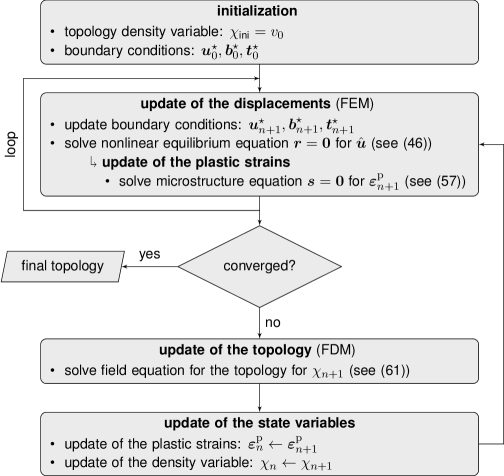
Figure 1: Flowchart of the proposed numerical implementation of the thermodynamic topology optimization including plasticity.

4 Numerical results

We present several aspects of our novel thermodynamic topology optimization including plasticity by investigation of various numerical experiments. We begin with the presentation of the general functionality of the proposed surrogate material model for plasticity on the material point level. Afterwards, we show the impact of the material model on the optimized construction parts by means of analyzing several quasi-2D and 3D boundary value problems. All results are based on our numerical implementation [24] in Julia [7]. We use the material parameter for steel summarized in Tab. 1.

Table 1: Material parameters for steel.

Young’s modulus	$E_{0}$	$210\,000$	[$\mathrm{MPa}$]			slope of hardening	$h$/$h_{1}$	$1000$	[$\mathrm{MPa}$]
Poisson’s ratio	$\nu$	$0.3$	[-]			initial slope of hardening	$h_{0}$	$40\,000$	[$\mathrm{MPa}$]
yield stress	$\sigma^{\mathrm{Y}}_{\mathrm{exp}}$	$300$	[$\mathrm{MPa}$]			transition of hardening	$\kappa$	$300$	[-]

The yield stress for modelling results from the material parameter with $\sigma^{\mathrm{Y}}=\sqrt{2/3}\,\sigma^{\mathrm{Y}}_{\mathrm{exp}}$. The hardening parameters are chosen according to [23]. An overview of the different material models used in the following is given in Fig. 2 on material point level.

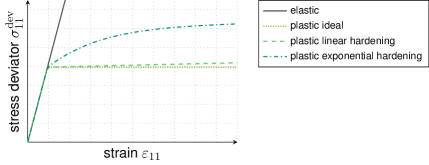
Figure 2: Overview of material behavior: elastic and different types of plastic models.

4.1 Surrogate model for plasticity

The computation of plastic strains takes place at the microstructural level. To investigate the results of the proposed surrogate material model for plasticity, we present a first result at the material point and thus without topology optimization. Consequently, we prescribe the strain as linear function of $100$ load steps with tension and pressure loading and unloading. For this, we determine the strain tensor depending on the load step $l$ according to

(62) $$\boldsymbol{\varepsilon}(l)=\varepsilon_{11}(l)\,\left(\begin{array}[]{rrr}1&0.6&0.6\\ 0.6&-\nu&-0.1\\ 0.6&-0.1&-\nu\\ \end{array}\right)\,.$$

To present a result that is representative, the diagonal entries correspond to the material parameters given above (Tab. 1), i. e., we use the Poisson’s ratio of steel, and the shear components have been chosen randomly. The maximum value of the component in $11$-direction is set to $\varepsilon_{11,\max}(l)=0.005\,[-]$. The numerical results for the surrogate model for plasticity at the material point are given as stress/strain diagram exemplary for ideal plasticity.

Matching the scalar-valued comparison of the indicator function, the von Mises stresses are plotted above the norm of strains in Fig. 3. It indicates that the intended material behavior is displayed: first, the stress/strain curve of the proposed material model increases linearly in the elastic region. The end points of the elastic region are indicated by $\varepsilon_{\mathrm{exp}}^{\mathrm{Y}}$ and $\sigma^{\mathrm{Y}}_{\mathrm{exp}}$, respectively.

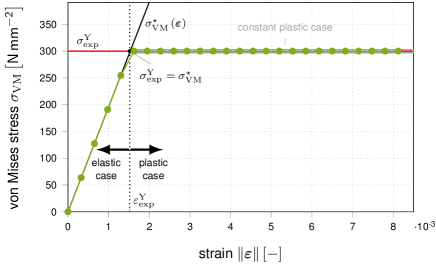
Figure 3: Overview of the decision criteria for microstructural update cases using the example of ideal plasticity. The update of the plastic strains is executed if the plastic case is detected.

Then, the stress reaches the yield stress level $r$, here $\sigma^{\mathrm{Y}}_{\mathrm{exp}}$, in the plastic case. This behavior coincides to classical plasticity models. However, the remarkable difference is that the unloading case is also included in Fig. 3. Here, no hysteresis is observed but with decreasing strains the stress level is maintained until the strains indicate the elastic region. The result is thus independent of the unloading history. Correspondingly, the increase or decrease of plastic strains in the surrogate material model directly reacts on the increase or decrease of strains in the plastic case.

An important difference of our novel surrogate model for dissipation-free plasticity to classical elasto-plastic material models is that we do not formulate our model by using an ordinary differential equation. Consequently, path-dependence, as intended, is excluded in our model. Of course, there exists no proof that the different formulations, ODE for classical models vs. algebraic equation for our model, give same results even when only the loading case is considered for which we demand a similar material behavior. To investigate the quality of our novel surrgate model in this regard, we compare the surrogate material model and the hysteresis curve for a classical elasto-plastic model accounting for one component of the stress/strain state. Thus, both curves are shown in Fig. 4.

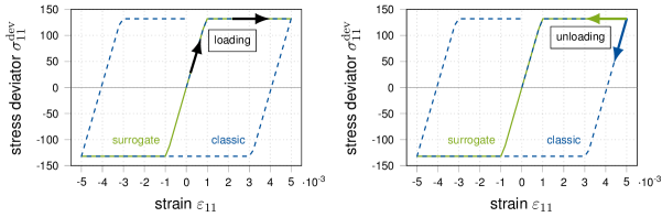
Figure 4: Material point curve of the surrogate model and the classic elasto-plastic model for ideal plasticity. The new idea about the surrogate model is the “virtual” compared to the physical unloading.

Here, the behavior for loading and unloading can be observed in greater detail. As a result, the surrogate material model deviates from the purely physical classical elasto-plastic material behavior exactly as intended. Both models show the identical physical loading path but differ in unloading. While the classic model results in the typical hysteresis by dissipation during physical unloading, the virtual unloading follows back the loading path in our surrogate model. Therefore, the proposed surrogate model displays a physically reasonable plastic material behavior but without considering dissipation.

Remark: It is worth mentioning that we obtain exactly the behavior as for hyperelastic surrogate model in the 1D case. However, this holds true for each individual tensor component which differ in different stress levels in the plastic regime which are determined by the specific strain state. Consequently, our surrogate material model yields the intended results also for the 3D case in which the calibration of a hyperelastic model is a very challenging task, if possible at all.

Another investigation of the quality of the surrogate model is discussed by the results of a FEM simulation. To this end, we choose a fix density distribution of the clamped beam (defined in Sec. 4.2.1) given by optimization results (Fig. 9, $1$ loop). For this structure and boundary value problem, both for the surrogate model and classic elasto-plasticity a simulation is applied in which we ramp the maximum displacement up over $20$ load steps. All computations are performed for all plasticity types: ideal, linear hardening and exponential hardening. The resulting distribution of plastic strains and its relative difference is plotted in Fig. 5.

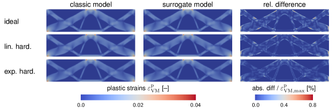
Figure 5: Comparing the classic and the surrogate model by a FEM simulation on a given structure which is loaded in $20$ steps to the maximum load of $u=$-0.05\text{\,}\mathrm{mm}$$ accounts for different plastic characteristics show very small differences in the plastic strains.

The maximum deviation is always less than $1\text{\,}\mathrm{\char 37\relax}$. Considering the mathematical difference of the two models, the difference of computed plastic strain is unexpectedly low.

This allows us to validate that the surrogate model along with its implementation address the proposed aspects on the material point level and also confirms accuracy within the FEM.

4.2 Optimization results with surrogate model for plasticity

4.2.1 Benchmark problems and optimization parameters

To demonstrate the functionality of the consideration of plasticity in the thermodynamic topology optimization, several boundary value problems are tested. To this end, we present all considered design spaces with the respective boundary conditions and symmetry planes.

The clamped beam in Fig. 7 is fixated at both sides and chosen in analogy to Maute et al. [27]. The quasi-2D classical Messerschmitt-Bölkow-Blohm (MBB) beam shown in Fig. 7 is simply supported at the lower corner nodes. Both models are loaded centrally (without symmetry plane) on the design space from above.

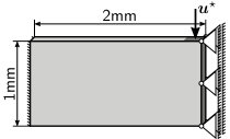
Figure 6: Dimensions of design space and boundary value conditions for the quasi-2D clamped beam.

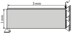
Figure 7: Dimensions of design space and boundary value conditions for the quasi-2D MBB.

As 3D example, we investigate the boundary value problem given in Fig. 8 and denote it as 3D cantilever. The corners of one side are fixated and the load is exerted at the bottom of the opposite side.

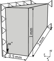
Figure 8: Dimensions of design space and boundary value conditions for the 3D cantilever.

All models are discretized by hexahedral finite element meshes with element edge size $e_{\mathrm{size}}$ and linear shape functions. The thickness of the quasi-2D models is discretized by one finite element with size $e_{\mathrm{size}}$.

It is worth mentioning that in contrast to topology optimization of linear elastic materials, our results depend in a non-linear way on the amplitude of load (which might be provided either by external forces or prescribed displacements). Here, the load conditions are applied as prescribed displacements $\boldsymbol{u}^{\star}$ where $\boldsymbol{u}^{\star}_{\max}$ is chosen such that plasticity evolves during optimization.

Our novel surrogate model allows to account for a physically reasonable computation of the plastic strains without repeating the entire loading history for each optimization step which is usually necessary to estimate the sensitivity. Therefore, it is worth mentioning that maximum loading, i. e., the loading for which the structure is optimized, can be employed instantaneously. This is a remarkable difference to other optimization schemes including plasticity. Since the solution of the finite element problem consumes the highest amount of computation time, our novel approach enables us to save numerical costs by reducing the number of necessary FEM simulations per iteration to even one or a few loops.

The density variable can be varied in the interval $\left[\chi_{\min},1\right]$ where the minimum value is set to $\chi_{\min}=$0.001$$. Therefore, the minimal material stiffness is given by $${10}^{-9}$\times\mathbb{E}_{0}$. The regularization parameter is chosen as $\beta=2\,e_{\mathrm{size}}^{2}\,${\mathrm{mm}}^{2}$$ and the viscosity for all simulations is set to $\eta=$15\text{\,}\mathrm{s}$$, corresponding to our previous work [17]. All necessary model and optimization parameters for the different boundary value problems are collected in Tab. 2.

Table 2: Model and optimization parameters.

boundary value problem	#elements	$e_{\mathrm{size}}\ [$\mathrm{mm}$]$	$\boldsymbol{u}^{\star}\ [$\mathrm{mm}$]$	$v_{0}\ [-]$	$\eta\ [$\mathrm{s}$]$	$\beta\ [${\mathrm{mm}}^{2}$]$
quasi-2D clamped beam	$5000$	$0.02$	$0.05$	$0.5$	$15$	$0.80\text{\times}{10}^{-3}$
quasi-2D MBB beam	$4800$	$0.025$	$0.02$	$0.5$	$15$	$1.25\text{\times}{10}^{-3}$
3D cantilever	$26\,364$	$1\text{/}26$	$0.06$	$0.15$	$15$	$2.96\text{\times}{10}^{-3}$

As mentioned, the stresses lag behind the strains due to the staggered process. In order to better approximate physics, we compute $15$ FEM simulations within one optimization iteration and before updating the topology for the next time. This additional simulations are denoted as loops in the following.

The illustrations of the field data are created with Paraview [3]. Even if the models make use of symmetry planes, the results are presented as whole (mirrored) in some instances. The resultant structures are obtained by using the isovolume filter for the density variable $\chi$ with the minimum threshold set to $0.5$. This is the average value of the interval in which $\chi$ has been defined.

4.3 Optimal structures

We investigate the impact of inclusion of plasticity on the resultant optimal structure. To this end, the optimization results are compared with results of thermodynamic topology optimization for a linear elastic material behavior. This can be achieved while setting the yield stress to an unphysically high value, i. e. $\sigma^{\mathrm{Y}}_{\mathrm{exp}}=$500\,000\text{\,}\mathrm{MPa}$$. This ensures that no plastic deformation is active since the von Mises norm of the stress is below this value for all boundary value problems considered. The results obtained from this elastic optimization are, of course, consistent with results obtained in our previous publications, cf. [17], for instance. All structures are presented for the converged iteration step. The structures with shades of green correspond to the thermodynamic topology optimization including plasticity (ideal or hardening) whereas the gray structure is the result for a purely linear elastic topology optimization.

Due to loading, high plastic strains may occur in the entire design space. Two result regions with lower stress intensities in topology are possible: i) thicker cross-section areas reduce the maximum value of the averaged stress such that the remaining stress is limited by the yield criterion $r$, or ii) vanishing substructures because no stresses occur for void material. For an example of the distribution of plastic strains, we refer to Sec. 4.5 in which a structure is computed where the highest stresses and thus plastic deformations are present at the constrained boundaries in terms of external loading and supports. Consequently, we observe thicker member sizes here, cf. the center and supports of the clamped beam in Fig. 9 and the center of the MBB in Fig. 10.

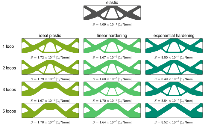
Figure 9: Overview of optimized structures and stiffness $S$ for the clamped beam with the surrogate material model accounting for different plastic characteristics and several numbers of inner loops.

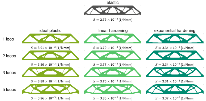
Figure 10: Overview of optimized structures and stiffness $S$ for the MBB with the surrogate material model accounting for different plastic characteristics and several numbers of loops.

Otherwise, high plastic strains occur in the complete middle part of the design space of the clamped beam. For this reason, a large void area below the truss corresponding to the loading can be seen in Fig. 9. This void region is even wider than in the elastic optimization result. For an increasing number of FEM loops even the lower trusses disappear completely. This has an impact on the total structure regarding the general topology: due to prescribed total structure volume, the angles and thicknesses of some bars change significantly for the plastic optimization. Consequently, remarkably different structures are computed when plastic material behavior is considered.

Based on the staggered optimization process, stresses are overestimated. Therefore, we propose to achieve stresses that are more physical due to the increasing number of additional FEM loops. Thereby, the displacement field follows the stresses and therefore the plastic strains better reflects the physical reality. The optimization results observed for the clamped beam and the MBB confirm the assumed influence, see Fig. 9 and Fig. 10 from left to right. Both thicker trusses with reduction of structure and rearrangement of thickness in further trusses seem possible. As a result, plastic strains, corresponding to the displacement field, are crucial for the optimized structures.Therefore, the number of loops need to be chosen wisely.

Remark: It should be mentioned, that the number of $15$ loops used here is significantly less than the number of load steps required for a path-dependent classic plasticity model, e. g. $20$ load increments in Fig. 5. Therefore, this proposed method is still fast and efficient.

A special characteristic of our approach is that we can model both ideal plasticity and hardening. Therefore, we are able to determine that specifications of plasticity result in different structures. Some structures show small differences but especially with $3$ loops differences are obvious. This can be seen for the clamped beam in Fig. 9 and for the MBB in Fig. 10 in a vertical comparison. For instance, the MBB with $3$ loops has more truss elements for linear hardening than for ideal plasticity and even more with exponential hardening. This means, a precisely defined material behavior is important. Therefore, it is a great advantage that real material behavior can be reproduced in an accurate way by this approach, and can be entered in the optimization process directly in this way.

The optimization results of the 3D cantilever seen in Fig. 11 proves the functionality and applicability of our approach for fully 3D boundary problems.

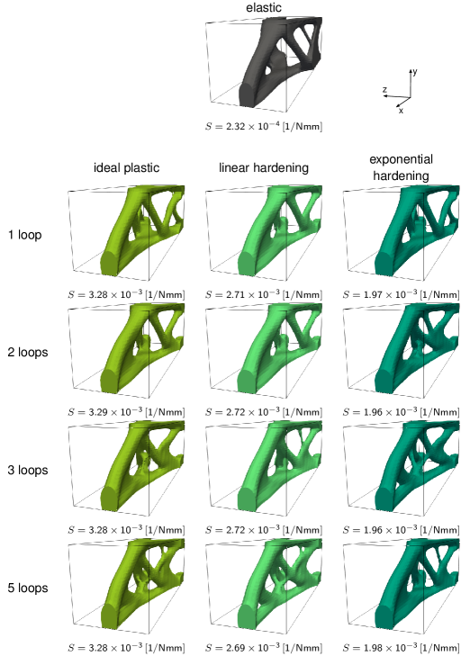
Figure 11: Overview of optimized structures and stiffness $S$ for the 3D cantilever with the surrogate material model accounting for different plastic characteristics and several numbers of loops.

4.4 Convergence behavior

Another aspect of analysis is to discuss the evolution of the optimization objective which is to minimize the compliance of the structure. Since a compliance minimization analogously causes a stiffness maximization, we use the latter for presentation. The stiffness is computed in analogy to other works on topology optimization by $S=1/\boldsymbol{f}\cdot\hat{\boldsymbol{u}}$. Consequently, we expect a decreasing function for $S$ when the reaction force increases during the evolution of the structure. The order of magnitude of stiffness is very different for elastic and plastic optimization. For a convincing representation a logarithmic stiffness axis is chosen. We define convergence as soon as the relative stiffness changes less than $1\text{\times}{10}^{-5}$ for the first time and less than $1\text{\times}{10}^{-4}$ for further three succeeding iteration steps. This rather strict convergence criterion is chosen to exclude a wrong detection of convergence in the plastic case.

The stiffness and iteration step of convergence is plotted for the clamped beam and the MBB with $3$ loops in Fig. 12, for instance.

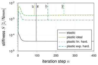
(a) Clamped beam (3 loops)

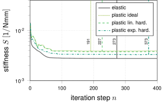
(b) MBB (3 loops)

Figure 12: Convergence of stiffness evolution during the optimization process. The first time that the convergence criterion has been reached is indicated by a vertical line.

We still see the usual evolution of the stiffness during topology optimization which is that the stiffness increases while a discrete black/white structure evolves. In the elastic case, the maximum stiffness converges towards a constant value.

The onset of plasticity includes remarkable reduction of stiffness since locally higher strains do not result in higher or stress: the yield stress $\sigma^{\mathrm{Y}}$ is the fixed upper limit for ideal plasticity, and the increase of stress is slowed down with hardening. This is a physically reasonable behavior. Therefore, the stiffness of structures including plasticity is lower than of those which behave purely elastically. This becomes particularly clear with the clamped beam in Fig. 12(a) where larger values of plastic strains are observed. In general, the (absolute value of the) differences in the stiffness plots corresponds to the dissipated energy due to the plastic formation of deformations.

Furthermore, the plastic strains are even lower for hardening than for ideal plasticity. This is caused by the yield criterion $r$ which allows the stresses to increase in a defined manner with hardening. Therefore, the plots also show a greater stiffness especially for exponential hardening. Structures with a higher stiffness are thus more similar to elastically optimized structures, cf. the clamped beam in Fig. 11 with exponential hardening.

It is remarkable that sometimes plastic optimizations converge in less iteration steps than the elastic optimizations, cf. Fig. 12. The number of convergence iterations is a major factor for the difference in computation time in plastic and elastic optimizations. This can be seen by comparing the runtimes for elastic and plastic optimizations with $1$ loop in Tab. 3.

Table 3: Convergence iteration steps and relative runtime according to elastic optimization.

boundary value problem	type of plasticity	convergence iteration step		rel. runtime
		1 loop	3 loops	1 loop	3 loops
	elastic	$96$		$1.0$
	ideal plastic	$167$	$87$	$3.25$	$5.12$
	linear hardening	$295$	$242$	$6.15$	$14.75$
quasi-2D clamped beam	exp. hardening	$237$	$157$	$4.96$	$9.00$
	elastic	$273$		$1.0$
	ideal plastic	$292$	$191$	$1.10$	$2.26$
	linear hardening	$201$	$227$	$0.71$	$2.50$
quasi-2D MBB	exp. hardening	$125$	$373$	$0.44$	$3.64$

It is obvious that computation time also increases with the number of loops (cf. Tab. 3 for $3$ loops) which remain less than $5$ loops in our method. Therefore, with the surrogate model the needed computational resources for a plastic optimization is comparable to an elastic optimization which is applicable in engineering practice.

4.5 Structure evolution during the optimization process

The evolution of the structure and the plastic strains $\boldsymbol{\varepsilon}^{\mathrm{p}}$ during the optimization process is exemplary presented for the clamped beam with $3$ loops with ideal plasticity and linear hardening in Fig. 13.

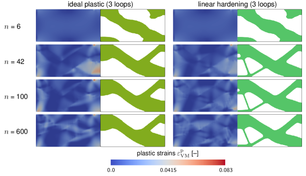
Figure 13: Evolution of increasing/decreasing plastic strains and structure during the optimization process for the clamped beam (3 loops) with ideal plasticity and linear hardening.

Especially for the clamped beam with linear hardening, the structure and void areas under the influence of plastic strains can be observed, as explained in Sec. 4.3. Furthermore, we see that the value of plastic von Mises strains is lower for hardening than for ideal plasticity for the optimization of the clamped beam.

It is worth mentioning that the amount of plastic strains also reduces during the optimization while stiffness increases and thus strains are locally reduced (again). This can be seen when comparing the iteration steps $n=42$ and $n=100$ at the area of external displacement and support for ideal plasticity in Fig. 13. Therefore, it is a crucial property of the proposed material model to reduce plasticity without dissipation. This proves that the proposed surrogate material model for plasticity without dissipation operates as expected during the optimization process. It is thus possible to consider the plastic strain evolution simply by considering the current strain while avoiding the repeated computation of the entire loading path.

5 Conclusion and outlook

A novel approach to the thermodynamic topology optimization including plasticity was presented. To avoid the computation of a complete load path for estimating the plastic strain state in every optimization step, a novel surrogate material model was developed. To this end, the model was constructed to be dissipation-free such that the plastic strains result from pure energy minimization. The resultant system of governing equations followed as stationarity conditions from an extended Hamilton functional. The system comprised the field equations for the displacements and the density variable, and an algebraic equation for the plastic strains. In the algebraic equation for plastic strains, arbitrary types of plasticity can be included by defining the related yield criterion: exemplary we used ideal plasticity, linear hardening and exponential hardening. For the numerical implementation, we employed the neighbored element method for solving the weak form of the balance of linear momentum and the strong form of the evolution equation for the density variable. Thereby, optimization is solved as evolutionary process in a staggered manner. We presented both a material point and FEM investigation to demonstrate the general functionality of the novel material model and various finite boundary value problems for optimization. Significant deviations between optimized structures for purely elastic materials and the surrogate model for plastic deformations could be detected. Also differences can be observed for different numbers of FEM loops during one iteration step as well as with ideal plasticity, linear or exponential hardening. All optimizations result in reliable convergence and with a suitable number of iteration steps. During the optimization process, our surrogate material model allows both to predict the microstructural state both for increasing and decreasing strain states due to topology optimization: the plastic strains always correspond to a state evolved during pure loading as is the case for the optimized component during real application. A remarkable numerical advantage is a computation runtime for the optimization including plasticity is comparable to that for an elastic optimization.

These findings provide the following insights for future research: with the staggered process, the physical reality is always mapped with a time delay and the optimization is based on these results. We tried to compensate this delay by additional FEM loops within one optimization iteration. Therefore, it would be particularly interesting for further research to investigate a monolithic treatment of thermodynamic topology optimization.

Appendix A Derivation of the surrogate material model

From the stationarity condition (14)₂, the Lagrange parameters $\lambda_{\mathrm{\sigma}}$ and $\lambda_{\mathrm{V}}$ need to be computed. Therefore, let us reformulate (2.2) such that we can compute $\lambda_{\mathrm{\sigma}}$ and $\lambda_{\mathrm{V}}$ analytically. To this end, both sides of (2.2) are double contracted by the deviator operator $\mathbb{P}$ from the left hand side. This yields

(63) $$-\boldsymbol{\sigma}^{\mathrm{dev}}-\lambda_{\mathrm{\sigma}}\left[\frac{\boldsymbol{\sigma}^{\mathrm{dev}}}{\left\lVert\boldsymbol{\sigma}^{\mathrm{dev}}\right\rVert}:\mathbb{P}:\chi^{3}\,\mathbb{E}_{0}+\mathbb{P}:\frac{\partial r}{\partial\boldsymbol{\varepsilon}^{\mathrm{p}}}\right]=0$$

where we used $\mathbb{P}:\boldsymbol{\sigma}^{\mathrm{dev}}=\boldsymbol{\sigma}^{\mathrm{dev}}$ and $\mathbb{P}:\boldsymbol{I}=\boldsymbol{0}$. Furthermore, it holds $\boldsymbol{\sigma}^{\mathrm{dev}}:\mathbb{P}:\chi^{3}\,\mathbb{E}_{0}=\boldsymbol{\sigma}^{\mathrm{dev}}:\chi^{3}\,\mathbb{E}_{0}$. Afterwards, we double contract both sides by the stress deviator $\boldsymbol{\sigma}^{\mathrm{dev}}$ from the right-hand side, yielding

(64) $$-\boldsymbol{\sigma}^{\mathrm{dev}}:\boldsymbol{\sigma}^{\mathrm{dev}}-\lambda_{\mathrm{\sigma}}\left[\frac{\boldsymbol{\sigma}^{\mathrm{dev}}}{\left\lVert\boldsymbol{\sigma}^{\mathrm{dev}}\right\rVert}:\chi^{3}\,\mathbb{E}_{0}:\boldsymbol{\sigma}^{\mathrm{dev}}+\mathbb{P}:\frac{\partial r}{\partial\boldsymbol{\varepsilon}^{\mathrm{p}}}:\boldsymbol{\sigma}^{\mathrm{dev}}\right]=0\,.$$

Finally, we insert the constraint $\boldsymbol{\sigma}^{\mathrm{dev}}:\boldsymbol{\sigma}^{\mathrm{dev}}=\left\lVert\boldsymbol{\sigma}^{\mathrm{dev}}\right\rVert^{2}=r^{2}$ and $\left\lVert\boldsymbol{\sigma}^{\mathrm{dev}}\right\rVert=r$, respectively, and also account for $\mathbb{P}:\boldsymbol{\sigma}^{\mathrm{dev}}=\boldsymbol{\sigma}^{\mathrm{dev}}$ which gives us

(65) $$\lambda_{\mathrm{\sigma}}=-\frac{r^{3}}{\displaystyle\boldsymbol{\sigma}^{\mathrm{dev}}:\chi^{3}\,\mathbb{E}_{0}:\boldsymbol{\sigma}^{\mathrm{dev}}+\frac{\partial r}{\partial\boldsymbol{\varepsilon}^{\mathrm{p}}}:\boldsymbol{\sigma}^{\mathrm{dev}}\,r}\,.$$

To compute the Lagrange parameter $\lambda_{\mathrm{V}}$, we double contract (2.2) with $\boldsymbol{I}$ from the right-hand side. This results in

(66) $$-\boldsymbol{\sigma}:\boldsymbol{I}-\lambda_{\mathrm{V}}\,\boldsymbol{I}:\chi^{3}\,\mathbb{E}_{0}:\boldsymbol{I}=0$$

where we used $\mathbb{P}:\boldsymbol{I}=0$ and $\partial r/\partial\boldsymbol{\varepsilon}^{\mathrm{p}}=0$ in case of ideal plasticity or

(67) $$\frac{\partial r}{\partial\boldsymbol{\varepsilon}^{\mathrm{p}}}:\boldsymbol{I}=\frac{\partial r\left(\left\lVert\boldsymbol{\varepsilon}^{\mathrm{p}}\right\rVert\right)}{\partial\left\lVert\boldsymbol{\varepsilon}^{\mathrm{p}}\right\rVert}\,\frac{\partial\left\lVert\boldsymbol{\varepsilon}^{\mathrm{p}}\right\rVert}{\partial\boldsymbol{\varepsilon}^{\mathrm{p}}}:\boldsymbol{I}=\frac{\partial r\left(\left\lVert\boldsymbol{\varepsilon}^{\mathrm{p}}\right\rVert\right)}{\partial\left\lVert\boldsymbol{\varepsilon}^{\mathrm{p}}\right\rVert}\,\frac{\boldsymbol{\varepsilon}^{\mathrm{p}}:\boldsymbol{I}}{\left\lVert\boldsymbol{\varepsilon}^{\mathrm{p}}\right\rVert}=r^{\prime}\,\frac{\boldsymbol{\varepsilon}^{\mathrm{p}}:\boldsymbol{I}}{\left\lVert\boldsymbol{\varepsilon}^{\mathrm{p}}\right\rVert}=0$$

due to $\boldsymbol{I}:\boldsymbol{\varepsilon}^{\mathrm{p}}=0$, respectively. Inserting the constraint $\boldsymbol{\sigma}:\boldsymbol{I}=\boldsymbol{I}:\chi^{3}\,\mathbb{E}_{0}:\boldsymbol{\varepsilon}$ results in

(68) $$\lambda_{\mathrm{V}}=-\frac{\boldsymbol{I}:\chi^{3}\,\mathbb{E}_{0}:\boldsymbol{\varepsilon}}{\boldsymbol{I}:\chi^{3}\,\mathbb{E}_{0}:\boldsymbol{I}}\,.$$

Then, we finally find

$$\boldsymbol{s} := -\boldsymbol{\sigma}+\frac{r^{3}}{\displaystyle\boldsymbol{\sigma}^{\mathrm{dev}}:\chi^{3}\,\mathbb{E}_{0}:\boldsymbol{\sigma}^{\mathrm{dev}}+\frac{\partial r}{\partial\boldsymbol{\varepsilon}^{\mathrm{p}}}:\boldsymbol{\sigma}^{\mathrm{dev}}\,r}\,\left[\frac{\boldsymbol{\sigma}^{\mathrm{dev}}:\chi^{3}\,\mathbb{E}_{0}}{r}+\frac{\partial r}{\partial\boldsymbol{\varepsilon}^{\mathrm{p}}}\right]$$

$$+\frac{\boldsymbol{I}:\chi^{3}\,\mathbb{E}_{0}:\boldsymbol{\varepsilon}}{\boldsymbol{I}:\mathbb{E}_{0}:\boldsymbol{I}}\,\boldsymbol{I}:\mathbb{E}_{0}=\boldsymbol{0}$$

which constitutes as the governing equation for the plastic strains, cf. (2.2).

Appendix B Finite element method according to Ferrite

A possible implementation of the thermodynamic topology optimization including plasticity by use of the Ferrite package [10] and the tensors package [11] is presented in the Alg. 2 and Alg. 3. This algorithm is deduced from our published Julia code in [24].

Algorithm 2 Finite element implementation in Ferrite [10]

while true do

     

     for each $element\in mesh$ do $\triangleright$ repeat for each element

         

         call $\text{reinit!}(mesh,elementvalues)$ $\triangleright$ element values

         

         for each $ip$ $\in$ $element$ do $\triangleright$ repeat for each integration point

              

              compute $\boldsymbol{\varepsilon}=\text{function\_symmetric\_gradient}(elementvalues,ip,\boldsymbol{u}_{e})$ $\triangleright$ strains

              

              compute $\boldsymbol{\sigma}$, $\boldsymbol{\varepsilon}^{\mathrm{p}}$ and $\mathbb{D}$ $\triangleright$ material state and tangent

              

              compute $\Omega^{\star}=\text{getdetJdV}(elementvalues,ip)$ $\triangleright$ weighted volume fraction

              

              for $i$ to number base shape functions do $\triangleright$ repeat for number of base shape functions

                  

                  compute $\boldsymbol{B}^{\mathrm{T}}=\text{shape\_symmetric\_gradient}(elementvalues,ip,i)$

                  $\triangleright$ derivative of shape functions

                  

                  compute $\boldsymbol{r}_{e}\left[i\right]+=\left(\boldsymbol{B}^{\mathrm{T}}:\boldsymbol{\sigma}\right)\,\Omega^{\star}$ $\triangleright$ element residual vector

                  

                  for $j$ to number base shape functions do $\triangleright$ repeat for number of base shape functions

                       

                       compute $\boldsymbol{B}=\text{shape\_symmetric\_gradient}(elementvalues,ip,j)$

                       $\triangleright$ derivative of base shape function

                       

                       compute $\boldsymbol{K}_{e}\left[i,j\right]+=\left(\boldsymbol{B}^{\mathrm{T}}:\mathbb{D}:\boldsymbol{B}\right)\ \Omega^{\star}$ $\triangleright$ element stiffness matrix

                       

                  end for

                  

              end for

              

              compute $\boldsymbol{r}_{e}=\boldsymbol{r}_{e}-\boldsymbol{f}_{e,\mathrm{ext}}$ $\triangleright$ apply external forces

              

         end for

         

         call $\text{assemble!}(assembler,\boldsymbol{K}_{e},\boldsymbol{r}_{e})$ $\triangleright$ global stiffness matrix, global residual vector

         

     end for

Algorithm 3 Continuation of the finite element method in Ferrite [10]

     

     call $\text{apply\_zero!}(\boldsymbol{K},\boldsymbol{r},constraints)$ $\triangleright$ apply boundary conditions

     

     if $\left\lVert\boldsymbol{r}\right\rVert<\text{tol}$ then break

     end if$\triangleright$ check convergence criterion

     

     update $\displaystyle\boldsymbol{u}_{i+1}=\boldsymbol{u}_{i}-\frac{\boldsymbol{r}}{\boldsymbol{K}}$ $\triangleright$ displacement vector

     

     update $i=i+1$ $\triangleright$ next Newton iterator

     

end while

References

- [1] Ryan Alberdi and Kapil Khandelwal. Topology optimization of pressure dependent elastoplastic energy absorbing structures with material damage constraints. Finite Elements in Analysis and Design, 133:42–61, 2017.
- [2] Oded Amir. Stress-constrained continuum topology optimization: a new approach based on elasto-plasticity. Struct Multidisc Optim, 55:1797–1818, 2016.
- [3] Utkarsh Ayachit. The ParaView Guide: A Parallel Visualization Application, www.paraview.org. Kitware, 2015.
- [4] Alexander Bartels, Patrick Kurzeja, and Jörn Mosler. Cahn–hilliard phase field theory coupled to mechanics: Fundamentals, numerical implementation and application to topology optimization. Computer Methods in Applied Mechanics and Engineering, 383:113918, 2021.
- [5] M. P. Bendsøe. Optimal shape design as a material distribution problem. Structural Optimization, 1:193–202, 1989.
- [6] M. P. Bendsøe and O. Sigmund. Topology Optimization: Theory, Methods and Applications. Springer-Verlag Berlin Heidelberg, 2003.
- [7] Jeff Bezanson, Alan Edelman, Stefan Karpinski, and Viral B Shah. Julia: A fresh approach to numerical computing, www.julialang.org. SIAM Review, 59(1):65–98, 2017.
- [8] Matteo Bruggi and Pierre Duysinx. Topology optimization for minimum weight with compliance and stress constraints. Struct Multidisc Optim, 46:369–384, 2012.
- [9] T. E. Bruns, O. Sigmund, and D. A. Tortorelli. Numerical methods for the topology optimization of structures that exhibit snap-through. International Journal for Numerical Methods in Engineering, 55(10):1215–1237, 2002.
- [10] Kristoffer Carlsson, Fredrik Ekre, and Contributors. Ferrite.jl (Julia package), version: 0.3.0, date-released: 2021-03-25, https://github.com/ferrite-fem/ferrite.jl.
- [11] Kristoffer Carlsson, Fredrik Ekre, and Contributors. Tensors.jl (Julia package), version: 1.6.1, date-released: 2021-09-07, https://github.com/ferrite-fem/tensors.jl.
- [12] Joshua D. Deaton and Ramama V. Grandhi. A survey of structural and multidisciplinary continuum topology optimization: post 2000. Structural and Multidisciplinary Optimization, 49:1–38, 2014.
- [13] P. Duysinx and M. P. Bendsøe. Topology optimization of continuum structures with local stress constraints. International Journal for Numerical Methods in Engineering, 43:1453–1478, 1999.
- [14] Pierre Duysinx. Topology optimization with different stress limits in tension and compression. Third World Congress of Structural and Multidisciplinary Optimization (WCSMO3), 1999.
- [15] Felix Fritzen, Liang Xia, Matthias Leuschner, and Piotr Breitkopf. Topology optimization of multiscale elastoviscoplastic structures. International Journal for Numerical Methods in Engineering, 106:430–453, 2016.
- [16] Lothar Harzheim. Strukturoptimierung. Harri Deutsch, Frankfurt, 2008.
- [17] Dustin R. Jantos, Klaus Hackl, and Philipp Junker. An accurate and fast regularization approach to thermodynamic topology optimization. International Journal for Numerical Methods in Engineering, 117(9):991–1017, 2019.
- [18] Dustin Roman Jantos, Christopher Riedel, Klaus Hackl, and Philipp Junker. Comparison of thermodynamic topology optimization with simp. Continuum Mechanics and Thermodynamics, 31(2):521–548, 2019.
- [19] P. Junker, J. Makowski, and K. Hackl. The principle of the minimum of the dissipation potential for non-isothermal processes. Continuum Mechanics and Thermodynamics, 26(3):259–268, 2014.
- [20] Philipp Junker and Daniel Balzani. An extended hamilton principle as unifying theory for coupled problems and dissipative microstructure evolution. Continuum Mechanics and Thermodynamics, 33(4):1931–1956, 2021.
- [21] Philipp Junker and Daniel Balzani. A new variational approach for the thermodynamic topology optimization of hyperelastic structures. Computational Mechanics, (67):455–480, 2021.
- [22] Philipp Junker and Klaus Hackl. A variational growth approach to topology optimization. Structural and Multidisciplinary Optimization, 52(2):293–304, 2015.
- [23] Philipp Junker and Philipp Hempel. Numerical study of the plasticity-induced stabilization effect on martensitic transformations in shape memory alloys. Shape Memory and Superelasticity, 3(4):422–430, 2017.
- [24] Miriam Kick, Dustin R. Jantos, and Philipp Junker. Dataset: Implementation of thermodynamic topology optimization including plasticity in Julia, 2022.
- [25] Lei Li, Guodong Zhang, and Kapil Khandelwal. Topology optimization of energy absorbing structures with maximum damage constraint. International Journal for Numerical Methods in Engineering, 112:737–775, 2017.
- [26] Yangjun Luo and Zhan Kang. Topology optimization of continuum structures with drucker–prager yield stress constraints. Computers and Structures, 90–91:65–75, 2012.
- [27] K. Maute, S. Schwarz, and E. Ramm. Adaptive topology optimization of elastoplastic structures. Structural Optimization, 15:81–91, 1998.
- [28] P. B. Nakshatrala and D. A. Tortorelli. Topology optimization for effective energy propagation in rate-independent elastoplastic material systems. Computer Methods in Applied Mechanics and Engineering, 295:305–326, 2015.
- [29] Axel Schumacher. Optimierung mechanischer Strukturen: Grundlagen und industrielle Anwendungem. Springer, 2013.
- [30] Ole Sigmund and Kurt Maute. Topology optimization approaches. Structural and Multidisciplinary Optimization, 48(6):1031–1055, 2013.
- [31] C. Swan and I. Kosaka. Voigt–reuss topology optimization for structures with nonlinear material behaviors. International Journal for Numerical Methods in Engineering, 40:3785–3814, 1998.
- [32] Andreas Vogel and Philipp Junker. Adaptive thermodynamic topology optimization. Structural and multidisciplinary optimization, accepted for publication, 2020.
- [33] Mathias Wallin, Viktor Jönsson, and Eric Wingren. Topology optimization based on finite strain plasticity. Struct Multidisc Optim, 54:783–793, 2016.
- [34] Peter Wriggers. Nonlinear finite element methods. Springer Science & Business Media, 2008.
- [35] Liang Xia, Felix Fritzen, and Piotr Breitkopf. Evolutionary topology optimization of elastoplastic structures. Structural and Multidisciplinary Optimization, 55:569–581, 2017.
- [36] K. Yuge and N. Kikuchi. Optimization of a frame structure subjected to a plastic deformation. Structural Optimization, 10:197–2018, 1995.
- [37] Tuo Zhao, Eduardo N. Lages, Adeildo S. Ramos Jr., and Glaucio H. Paulino. Topology optimization considering the drucker–prager criterion with a surrogate nonlinear elastic constitutive model. Structural and Multidisciplinary Optimization, 62:3205–3227, 2020.
- [38] Tuo Zhao, Adeildo S. Ramos Jr., and Glaucio H. Paulino. Material nonlinear topology optimization considering the von mises criterion through an asymptotic approach: Max strain energy and max load factor formulations. International Journal for Numerical Methods in Engineering, 118:804–828, 2019.