Nuclear binding energy in holographic QCD

Abstract

Saturation of the nuclear binding energy is one of the most important properties of atomic nuclei. We derive the saturation in holographic QCD, by building a shell-model-like mean-field nuclear potential from the nuclear density profile obtained in a holographic multi-baryon effective theory. The numerically estimated binding energy is close to the experimental value.

I Introduction and summary

Holographic QCD provides effective theories via the AdS/CFT correspondence Maldacena:1997re ; Gubser:1998bc ; Witten:1998qj and allows us to calculate various observables of large $N_{c}$ QCD-like gauge theories. Nuclear physics is a challenging target of holographic QCD. The nuclear matrix model Hashimoto:2010je was proposed to be a unified model of nuclear physics inspired and derived by the AdS/CFT. Atomic nuclei are bound states of nucleons, which may allow an effective description in terms of baryons in holographic QCD. Nucleons are D-branes in the gravity side of the AdS/CFT, so the holographic theory of the nucleons is given by matrices, which is the basis of the nuclear matrix model. By the nuclear matrix model, several important properties of nuclei, including the nuclear radii Hashimoto:2011nm , nuclear spectra and magic numbers Hashimoto:2019wmg have been reproduced. In this paper, we study another important aspect of nuclei—the nuclear binding energy. We show that the nuclear matrix model also reproduces the saturation of the nuclear binding energy: the property that the nuclear binding energy per nucleon approaches a constant independent of the mass number $A$ at large $A$.

Nuclear states in holographic QCD are obtained as energy eigenstates of the nuclear matrix model. In the gravity side of the Sakai-Sugimoto model Sakai:2004cn ; Sakai:2005yt , the baryons correspond to the D4-branes called baryon vertices which are wrapped on the $S^{4}$-directions in the Witten geometry. The nuclear matrix model action is the low energy effective action of the baryon vertices. After the dimensional reduction for $S^{4}$-directions, the Hamiltonian of the nuclear matrix model for $A$ baryons is derived as Hashimoto:2010je

$$H_{\text{full}} =H-\mathrm{tr}A_{t}\left(Q_{U(A)}-N_{c}\right)\ ,$$ (1)

$$H =\frac{1}{2}\mathrm{tr}(\Pi^{I})^{2}+2\bar{\pi}_{\dot{\alpha}i}^{a}\pi^{\dot{\alpha}i}_{a}+\frac{1}{2}M^{2}\bar{w}^{\dot{\alpha}i}_{a}w_{\dot{\alpha}i}^{a}$$

$$\quad-4i\lambda\epsilon^{IJK}X_{A}^{J}X_{B}^{K}f^{AB}{}_{C}\,\bar{w}^{\dot{\alpha}i}_{a}(\tau^{I})_{\dot{\alpha}}{}^{\dot{\beta}}(t^{C})^{a}{}_{b}w_{\dot{\beta}i}^{b}$$

$$\quad-2\lambda\mathrm{tr}\left[X^{I},X^{J}\right]^{2}+\lambda\left(\bar{w}^{\dot{\alpha}i}(\tau^{I})_{\dot{\alpha}}{}^{\dot{\beta}}w_{\dot{\beta}i}\right)^{2}\ ,$$ (2)

where the indices $\{I,J,K,\cdots\}$, $\{i,j,k,\cdots\}$ and $\{\dot{\alpha},\dot{\beta},\dot{\gamma},\cdots\}$ label the three dimensional space, $SU(N_{f})$ flavors and $SU(2)$ spins, respectively. The other indices $\{A,B,C,\cdots\}$ and $\{a,b,c,\cdots\}$ stand for the adjoint and fundamental representations of the baryon $U(A)$ symmetry, and the trace is taken over the baryon $U(A)$ matrices. The fields $X^{I}$, $w$ and $\bar{w}$ are scalar fields which come from the D4-D4 and D4-D8 open strings, and $\Pi^{I}$, $\pi$ and $\bar{\pi}$ are their conjugate momenta, respectively.

The nuclear matrix model (2) gives bound states of nucleons and reproduces nuclear states Hashimoto:2019wmg . There is a difficulty in directly evaluating the nuclear binding energy by the nuclear matrix model. The nuclear binding energy is the energy difference between the nuclear bound state and the state at which all the constituent nucleons are infinitely far apart, while the nuclear matrix model is effective for nucleons close to each other. This difficulty is overcome once the following point is noticed: the saturation of the binding energy is only for large $A$. Most of the total binding energy comes from nucleons in lower energy levels, and that of the highest energy level which should be compared to the nucleon separated far away can be treated as zero approximately. Therefore, we can calculate the binding energy of the other nucleons and then the total binding energy by solving the nuclear matrix model.

Nuclear states in the matrix model are calculated in Hashimoto:2019wmg for small baryon numbers, but the procedure is not useful for large nucleon numbers. In the large $A$ limit, it is convenient to use the mean-field approximation. We here adopt the following strategy. First, starting with the nuclear density profile obtained by the nuclear matrix model Hashimoto:2011nm , we derive an effective mean-field potential which reproduces the density profile. This potential defines a holographic nuclear shell model, in which positions of nucleons are identified with diagonal eigenvalues of $X$ of the nuclear matrix model. Assuming that the binding energy for a nucleon at the fermi level is negligible, the total binding energy of the nucleus can be obtained by summing up all the energy of nucleons below the fermi energy in the holographic nuclear shell model. We calculate this nuclear binding energy and show that it reproduces the saturation property.

Since the nuclear matrix model can treat flavors, spins and orbital motion of baryons in a unified fashion, we can estimate the magnitude of the nuclear binding energy using the nucleon mass and the $\Delta$ mass as inputs. We find that the resultant numerical value turns out to be close to the experimental value of the binding energy. The result is quite nontrivial in view of the crude approximations employed in the holographic QCD.

The organization of this paper is as follows. In Sec. II, we construct a holographic nuclear shell model by deriving an effective potential from the nuclear density profile in the nuclear matrix model. In Sec. III, we calculate the holographic nuclear binding energy. Using the holographic nuclear shell model, we obtain the nuclear binding energy per nucleon and show that it is independent of $A$. We find that the binding energy is numerically close to the experimental value. Appendix A describes the details of the mass rescaling used in the calculus, and Appendix B adds a novel observation on the $A$-dependence of nuclear radii.

II Holographic nuclear shell model

First, we review the nuclear density profile of the nuclear matrix model Hashimoto:2011nm and check its consistency by confirming that the effect of $w$ is sub-leading. Then in Subsec. II.2 we inversely obtain the shell-model potential from the density profile. This serves as a holographic nuclear shell model, with which in Sec. III we calculate the nuclear binding energy.

II.1 Nuclear density in the nuclear matrix model

The nuclear density profile in the nuclear matrix model was derived in Hashimoto:2011nm by using the Ramond-Ramond charge density formula of D-branes Taylor:1999gq ,

$$\rho(x) =\frac{1}{(2\pi)^{3}}\int d^{3}k\,e^{-ik_{I}x^{I}}\left\langle\mathrm{tr}\exp\left[ik_{J}X^{J}\right]\right\rangle\ .$$ (3)

In the large $A$ and large $D$ limit, the nuclear matrix model effectively behaves as that with a harmonic potential since only the ladder diagrams contribute to the expectation value above. The density profile was calculated in Hashimoto:2011nm as

$$\rho(x) =\begin{cases}\displaystyle\frac{A}{\pi^{2}r_{0}^{2}\sqrt{r_{0}^{2}-r^{2}}}&(r<r_{0})\\ \rule{0.0pt}{18.0pt}0&(r>r_{0})\end{cases}$$ (4)

where $r$ is the radial coordinate in three dimensional space and $r_{0}$ is the surface radius which is related to the effective frequency $m$ as $r_{0}^{2}=2A/m$. In the derivation, the $w$-sector was ignored because the number of degrees of freedom of $w$ is ${\cal O}(A)$ while that of $X$ is ${\cal O}(A^{2})$. In this section we employ the ground state wave function developed in Hashimoto:2019wmg , and find that indeed the effect of the $w$-sector is sub-leading, to make sure that we can use (4) in the subsequent sections.

Let us evaluate the total energy including the contribution from the $w$-sector. The potential for $X^{I}$ can be approximated by a harmonic potential $(m^{2}/2)\mathrm{tr}(X^{I})^{2}$ as in Hashimoto:2019wmg and the energy of the orbital motion becomes

$$E=m\left(N_{X}+\frac{3}{2}\left(A^{2}-1\right)\right)\ ,$$ (5)

where $N_{X}$ is the number of excitations of $X^{I}$ and the second term comes from the zero-point fluctuations. The effective frequency of the orbital motion, $m$, is determined in a self-consistent fashion (see Appendix B of Hashimoto:2019wmg ) and is approximately given by

$$m^{2}=\frac{16A\lambda}{3(A^{2}-1)}\langle X^{I}_{A}X^{I}_{A}\rangle\ .$$ (6)

Here the expectation value in (6) is with the wave function given in Hashimoto:2019wmg , and we have some remarks. The gauge field $A_{t}$ behaves as a Lagrange multiplier and gives constraints that physical states must be in singlet of $SU(A)$ and have $U(1)$ charge of $Q_{U(1)}=N_{c}A$. Thus, the physical ground states must have $N_{c}A$ excitations of $w$. The energy of these excitations gives a correction to the nucleon mass, and also modifies the kinetic term of $X^{I}$ (see Appendix A for the details). Using an appropriate redefinition of $X^{I}$, the coupling constant $\lambda$ for $X^{I}$ in the Hamiltonian is replaced by

$$\lambda_{r}=\lambda\frac{M_{0}^{3}}{M_{N}^{3}}\ ,$$ (7)

where $M_{0}$ is the bare tension of the baryon vertex and $M_{N}$ is the nucleon mass which includes the energy of $w$ and $\bar{w}$.

As described in Hashimoto:2019wmg , for $A>2N_{f}$, because it is impossible to form a totally antisymmetric combination solely of $w$, excitations of $X^{I}$ should also be introduced in the wave function. A straightforward counting shows that $N_{X}$ is approximately given by $\left(3/2\right)^{7/3}A^{4/3}$ for large $A$. Thus, using the virial theorem $(1/2)m^{2}\langle\mathrm{tr}X^{2}\rangle={\langle V\rangle}=E/2$, an estimation of $\langle\mathrm{tr}X^{2}\rangle$ leads to

$$\langle\mathrm{tr}X^{2}\rangle=\frac{1}{m}\left[\left(\frac{3}{2}\right)^{\!7/3}\!\!\!\!A^{4/3}+\frac{3}{2}(A^{2}-1)\right]\ .$$ (8)

We find that, for large $A$, the first term which is the effect of the excitations due to the $w$-sector wave function is negligible (see Appendix B for the comparison of the sub-leading terms found here with the experimental data of the nuclear radius). Thus, the effective frequency for large $A$ is evaluated as

$$m^{3}=8\lambda_{r}A\ .$$ (9)

The density profile is given by (4) with $r_{0}=\lambda_{r}^{-1/6}A^{1/3}$.

II.2 Derivation of mean-field potential

In this subsection, we derive a mean-field effective potential for nucleons from the density distribution (4). The wave function of a non-relativistic fermion in an arbitrary spherically symmetric potential $V(r)$ is given by using the WKB approximation as

$$\psi=\frac{C}{r}p^{-1/2}(r)e^{i\int dr\,p(r)}Y_{lm}\ ,$$ (10)

where

$$p(r)=\sqrt{E-V(r)-\frac{l(l+1)}{r^{2}}}\ ,$$ (11)

and $Y_{lm}$ is the spherical harmonics. The wave function is suppressed very fast outside the classical turning point and approximately zero for

$$E<V(r)+\frac{l(l+1)}{r^{2}}\ .$$ (12)

The wave function must satisfy the quantization condition,

$$\int dr\,p(r)\simeq\pi n\ ,$$ (13)

with a positive integer $n$.

The constant $C$ is fixed by the normalization condition as

$$C^{-2}=4\pi\int\frac{dr}{p(r)}\ .$$ (14)

When the fermions occupy all the states below the fermi level at $E=E_{f}$, the density is obtained by the sum of the probabilities for those states as

$$\rho(r) =4\sum_{n,l,m}\left|\psi(r)\right|^{2}$$

$$\simeq\int_{V(r)}^{E_{f}}dE\int_{0}^{r^{2}(E-V(r))}(2l+1)dl\,\frac{dn}{dE}\frac{4C^{2}}{r^{2}p(r)}\ ,$$ (15)

where the sum is approximated by an integral when the number of states is sufficiently large. The factor $4$ in the first line comes from the sum over spins and flavors (proton and neutron). From the quantization condition, we obtain

$$\frac{dn}{dE}=\frac{1}{\pi}\frac{d}{dE}\int dr\sqrt{E-V(r)-\frac{l(l+1)}{r^{2}}}=\frac{1}{8\pi^{2}C^{2}}\ ,$$ (16)

and then, the density is calculated as

$$\rho(r) =\frac{2}{3\pi^{2}}\left(E_{f}-V(r)\right)^{3/2}\ .$$ (17)

Thus, for the nucleon density (4), the effective potential is inversely given by

$$V(r)=E_{f}-\frac{3^{2/3}A^{2/3}}{2^{2/3}r_{0}^{4/3}\left(r_{0}^{2}-r^{2}\right)^{1/3}}\ ,$$ (18)

for $r<r_{0}$. Since the density is approximately zero for $r>r_{0}$, this effective potential must be accompanied by a steep potential barrier at $r=r_{0}$.

The mean-field potential (18) defines our holographic nuclear shell model. In the next section, we use this potential to evaluate the nuclear binding energy.

III Holographic nuclear binding energy

III.1 Saturation

The shell-model effective potential (18) has the depth measured from the fermi level typically of

$$-V(r)\sim\frac{A^{2/3}}{r_{0}^{2}}\propto A^{0}\ .$$ (19)

This roughly implies that the nuclear binding energy per nucleon is independent of $A$. In this section, we evaluate the nuclear binding energy by the effective potential (18), more precisely.

It is expected that the binding energy of nucleons at the fermi level is very small. Hence we take $E_{f}=0$, and then, the binding energy per nucleon is approximately given by the average of the energy of each state. The total binding energy $B$ of a nucleus is a sum of the potential energy $B^{({\rm p})}$ and the kinetic energy $B^{({\rm k})}$, $B=B^{({\rm p})}+B^{({\rm k})}$. Below we calculate them separately.

The total potential energy $B^{({\rm p})}$ is given in terms of the density as

$$B^{({\rm p})}\equiv\left\langle V\right\rangle =4\pi\int r^{2}\rho(x)V(r)dr\ .$$ (20)

Then, the total potential energy for the effective potential (18) is evaluated as

$$B^{({\rm p})} =-\int\frac{2^{4/3}\cdot 3^{2/3}A^{5/3}r^{2}dr}{\pi r_{0}^{10/3}(r_{0}^{2}-r^{2})^{5/6}}$$

$$=-\frac{3^{8/3}\Gamma(\frac{7}{6})\,\lambda_{r}^{1/3}A}{2^{2/3}\sqrt{\pi}\,\Gamma(\frac{2}{3})}\ .$$ (21)

By using the virial theorem, the total kinetic energy $B^{({\rm k})}$ is given by

$$B^{({\rm k})}\equiv\frac{1}{2}\left\langle r\,V^{\prime}(r)\right\rangle =2\pi\int r^{3}\rho(x)V^{\prime}(r)dr\ .$$ (22)

Since the potential has very high potential barrier at $r=r_{0}$, $V^{\prime}(r)$ diverges there. In order to avoid this divergence, we introduce a regularization by modifying the potential as

$$V(r)=-\frac{3^{2/3}A^{2/3}}{2r_{0}^{5/3}}\frac{(r_{0}-r)^{n}}{\epsilon^{n+\frac{1}{3}}}$$ (23)

for $r>r_{0}-\epsilon$, and take the $\epsilon\to 0$ limit. Here, $n$ is the artifact of the regularization. It should be noted that the density should be modified simultaneously as

$$\rho(x)=\frac{A}{2^{1/2}\pi^{2}r_{0}^{5/2}}\frac{(r_{0}-r)^{\frac{3}{2}n}}{\epsilon^{\frac{3}{2}n+\frac{1}{2}}}\ ,$$ (24)

for consistency with (4). Then, the total kinetic energy is calculated as

$$B^{({\rm k})} =-\int_{0}^{r_{0}-\epsilon}\frac{2^{4/3}A^{5/3}r^{4}dr}{3^{1/3}\pi^{2}r_{0}^{10/3}(r_{0}^{2}-r^{2})^{11/6}}$$

$$\qquad-\int_{r_{0}-\epsilon}^{r_{0}}\frac{3^{2/3}A^{5/3}n(r_{0}-r)^{\frac{5}{2}n-1}dr}{2^{1/2}\pi r_{0}^{7/6}\epsilon^{\frac{5}{2}n+\frac{5}{6}}}$$

$$=\frac{3^{8/3}\sqrt{\pi}\,\lambda_{r}^{1/3}A}{2^{2/3}5\Gamma(\frac{2}{3})\Gamma(\frac{5}{6})}\ .$$ (25)

The final expression is, in fact, independent of the artifact of the regularization.

Thus, all together, the holographic nuclear binding energy $B$ in the large $A$ limit is obtained as

$$\frac{B}{A}=\left[\frac{3^{8/3}\Gamma(\frac{7}{6})}{2^{2/3}\sqrt{\pi}\,\Gamma(\frac{2}{3})}-\frac{3^{8/3}\sqrt{\pi}}{2^{2/3}5\Gamma(\frac{2}{3})\Gamma(\frac{5}{6})}\right]\lambda_{r}^{1/3}\ .$$ (26)

The important point is that this is independent of $A$, which shows the saturation of the nuclear binding energy—the property that the nuclear binding energy per nucleon approaches a constant for a large number of nucleons.

III.2 Numerical estimates

Let us numerically estimate the nuclear binding energy. We fix the parameters of the model $\lambda$ and $M$ by using the mass of a nucleon and that of $\Delta$ as inputs.

Together with the zero point fluctuation, the energy of the state with the isospin $I$ and the baryon number $A=1$ (a single baryon) in the nuclear matrix model Hashimoto:2019wmg is given by

$$E_{w}=\left(N_{c}+2N_{f}\right)M+\frac{4\lambda}{M^{2}}I(I+1)$$ (27)

where the first term is the zero point energy coming from all $N_{f}$ flavors, 2 spins and both $w$ and $\bar{w}$. In order to distinguish the mass of nucleons and $\Delta$, we took first order perturbative correction which is the last term of (2). By using $N_{c}=3$ and $N_{f}=2$, the nucleon mass $M_{N}$ and the $\Delta$ mass $M_{\Delta}$ are expressed as

$$M_{N} =M_{0}+7M+\frac{3\lambda}{M^{2}}\ ,$$ (28)

$$M_{\Delta} =M_{0}+7M+\frac{15\lambda}{M^{2}}\ ,$$ (29)

where $M_{0}$ is the bare tension of the baryon vertex,

$$M_{0}=\frac{\lambda_{\text{QCD}}N_{c}M_{KK}}{3^{3}\pi}=\frac{\lambda N_{c}^{2}}{3M^{2}}\ .$$ (30)

By using the experimental data, $M_{N}=939\ \mathrm{[MeV]}$ and $M_{\Delta}=1232\ \mathrm{[MeV]}$, the parameters of the nuclear matrix model are fixed as

$$\lambda =3.13\times 10^{5}\ \mathrm{[MeV^{3}]}\ , M =113\ \mathrm{[MeV]}\ .$$ (31)

Our holographic nuclear binding energy per nucleon (26) is evaluated as

$$\frac{B}{A}\simeq 9.66\ \mathrm{[MeV]}\ .$$ (32)

In experimental data, the naive average of the nuclear binding energy per nucleon measured is known to be roughly $B/A\simeq 8$ [MeV]. In another fitting of the experimental binding energy data by the empirical Bethe-Weizsäcker mass formula, the coefficient of the volume term (the large-$A$ leading term) shows $B/A\simeq 16$ [MeV]. Our numerical estimate (32) is close to the values of the experiments, which is a sufficiently good agreement as a nuclear model of holographic QCD.

Appendix A Mass rescaling

In this appendix, we study how the mass coefficient in the kinetic term of a generic non-relativistic action is scaled by quantum corrections to the total energy. This results in the scaling of the coupling (7).

A non-relativistic action of a free particle is obtained by the non-relativistic limit of a relativistic worldline action as

$$S =-m\int dt\,\sqrt{-\left(\dot{x}^{\mu}\right)^{2}}$$

$$\simeq\int dt\,\left[-m+\frac{1}{2}m\left(\dot{x}^{I}\right)^{2}+\cdots\right]\ ,$$ (33)

where $\mu$ is the spacetime index. To see the effect of the quantum corrections, it is convenient to introduce an einbein $e$ on the worldline,

$$S =\int dt\,\left[\frac{m}{2e}\left(\dot{x}^{\mu}\right)^{2}-\frac{1}{2}me\right]$$

$$=\int dt\,\left[\frac{m}{2e}\left(\dot{x}^{I}\right)^{2}-\frac{1}{2}m\left(e+e^{-1}\right)\right]\ .$$ (34)

Suppose we have a correction to the total energy from some other sector (such as $w$-sector in the nuclear matrix model). It would effectively introduce an additional cosmological constant term $\delta m$ on the worldline as

$$S =\int dt\,\left[\frac{m}{2e}\left(\dot{x}^{I}\right)^{2}-\frac{1}{2}m\left(e+e^{-1}\right)-e\,\delta m\right]\,.$$ (35)

With this correction, the equation of motion for the einbein $e$ is solved as

$$e^{2}=\frac{1-(\dot{x}^{I})^{2}}{1+(2\delta m)/m}\ ,$$ (36)

in which $(\dot{x}^{I})^{2}$ is negligible in the non-relativistic limit. Substituting this solution for the einbein, the corrected action (35) again takes the same form as (33), but now the mass $m$ is replaced by $M=m\sqrt{1+(2\delta m)/m}$. Thus, the correction to the total energy rescales the mass coefficient of the kinetic term as well as the cosmological constant on the worldline. This effect can also be interpreted as the rescaling of the einbein $e\simeq m/M$.

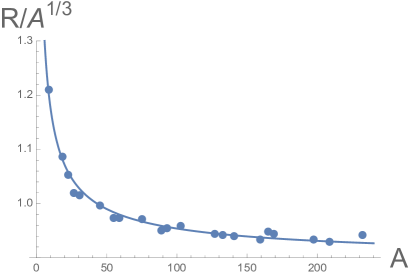
Figure 1: Experimental data table of the charge radius $R$ of all known mononuclidic elements. The solid line is the fitting curve (42) with the power $A^{-2/3}$ predicted by the holographic QCD. We find that the behavior is consistent.

With this rescaling of the mass in mind, we consider the correction to the mass in the $X$-sector in the nuclear matrix model. Introducing the einbein, the action for $X^{I}$ is naturally written as

$$S =\int dt\,\mathrm{tr}\left[\frac{1}{2e}\left(D_{t}X^{I}\right)^{2}+2e\,\lambda\left[X^{I},X^{J}\right]^{2}+\cdots\right]\ .$$ (37)

The natural kinetic term can be given by a rescaling of $X^{I}$ to that in the physical length scale $X^{I}_{\text{phys}}$ as

$$S =\int dt\,\mathrm{tr}\left[\frac{M_{0}}{2e}\left(D_{t}X^{I}_{\text{phys}}\right)^{2}\right.$$

$$\left.\quad+2e\,M_{0}^{2}\lambda\left[X^{I}_{\text{phys}},X^{J}_{\text{phys}}\right]^{2}+\cdots\right]\ ,$$ (38)

where the tension of the baryon vertex $M_{0}$ is given by (30). In this frame, we understand that the energy of $w$ gives the correction to the tension as (28), and modifies the einbein such that

$$e=\frac{M_{0}}{M_{N}}\ .$$ (39)

Using this corrected $e$ and redefining the coordinate as

$$X^{I}=M_{N}^{1/2}X^{I}_{\text{phys}}\ ,$$ (40)

we find that the action takes the same form as (37),

$$S =\int dt\,\mathrm{tr}\left[\frac{1}{2}\left(D_{t}X^{I}\right)^{2}+2\lambda_{r}\left[X^{I},X^{J}\right]^{2}+\cdots\right]\ ,$$ (41)

but with the rescaled coupling $\lambda_{r}\equiv e^{3}\lambda$, which is our (7).

Appendix B $A$-dependence of nuclear radius

With $m$ determined in (9), our evaluation (8) shows that for the nuclear radii growing as $A^{1/3}$ there exists a sub-leading correction in the large $A$ expansion. Expanding (8) for large $A$, we find that the sub-leading correction starts at $A^{-2/3}$. This peculiar power is the result of holographic QCD.

It is surprising that the nuclear experimental data indeed follow this $A^{-2/3}$ power law. In Fig. 1, we plot the experimental data table of the charge radius $R$ of all known mononuclidic elements. We fit the data with a function

$$\frac{R}{A^{1/3}}=c_{1}\left(1+c_{2}A^{-2/3}\right)\,$$ (42)

and find a consistent fit with $c_{1}=0.89$ [fm] and $c_{2}=1.5$ (the solid line in Fig. 1). As this fitting curve reproduces the data very well, we conclude that the sub-leading correction is given relatively by $A^{-2/3}$—the prediction of the holographic QCD is confirmed in experiments.

We may even quantitatively compare the coefficients $c_{1}$ and $c_{2}$ with the nuclear matrix model. Although in the model there could be some other sub-leading effect, here we simply assume the validity of (8) and look at how the nuclear radius changes in $A$. Using (8) itself, the mean-square radius of the atomic nucleus in the nuclear matrix model is

$$R_{\rm holo} \equiv\sqrt{\frac{1}{A}\Big{\langle}\mathrm{tr}(X^{I}_{\rm phys})^{2}\Big{\rangle}}\ ,$$ (43)

where $X^{I}_{\text{phys}}$ is related to $X^{I}$ in (8) by (40). Correcting (9) to the next-to-leading order, we have

$$m^{3}=8\lambda_{r}A+2^{5/3}3^{4/3}\lambda_{r}A^{1/3}\ .$$ (44)

Then, the coefficients $c_{1}$ and $c_{2}$ in the charge radius (43) are calculated as

$$c_{1}=\frac{3^{1/2}A^{1/3}}{2\lambda_{r}^{1/6}M_{N}^{1/2}}=\frac{M}{2\lambda^{2/3}}\,,\quad c_{2}=\frac{3^{1/3}}{2^{4/3}}\,.$$ (45)

Using the numerical parameters (31) of the nuclear matrix model, we find $c_{1}\simeq 2.4$ [fm] and $c_{2}\simeq 0.57$. These values are of the same order as those of the experiments, which is quite a good agreement in view of the crude approximations in the holographic QCD.

References

- (1) J. M. Maldacena, “The large N limit of superconformal field theories and supergravity,” Adv. Theor. Math. Phys. 2, 231 (1998) [Int. J. Theor. Phys. 38, 1113 (1999)] [arXiv:hep-th/9711200].
- (2) S. S. Gubser, I. R. Klebanov and A. M. Polyakov, “Gauge theory correlators from non-critical string theory,” Phys. Lett. B 428, 105 (1998) [arXiv:hep-th/9802109].
- (3) E. Witten, “Anti-de Sitter space and holography,” Adv. Theor. Math. Phys. 2, 253 (1998) [arXiv:hep-th/9802150].
- (4) K. Hashimoto, N. Iizuka and P. Yi, “A Matrix Model for Baryons and Nuclear Forces,” JHEP 1010, 003 (2010) doi:10.1007/JHEP10(2010)003 [arXiv:1003.4988 [hep-th]].
- (5) K. Hashimoto and T. Morita, “Nucleus from String Theory,” Phys. Rev. D 84, 046004 (2011) [arXiv:1103.5688 [hep-th]].
- (6) K. Hashimoto, Y. Matsuo and T. Morita, “Nuclear states and spectra in holographic QCD,” JHEP 12, 001 (2019) [arXiv:1902.07444 [hep-th]].
- (7) S. Aoki, K. Hashimoto and N. Iizuka, “Matrix Theory for Baryons: An Overview of Holographic QCD for Nuclear Physics,” Rept. Prog. Phys. 76, 104301 (2013) [arXiv:1203.5386 [hep-th]].
- (8) K. Hashimoto and N. Iizuka, “Three-Body Nuclear Forces from a Matrix Model,” JHEP 11, 058 (2010) [arXiv:1005.4412 [hep-th]].
- (9) K. Hashimoto, N. Iizuka and T. Nakatsukasa, “N-Body Nuclear Forces at Short Distances in Holographic QCD,” Phys. Rev. D 81, 106003 (2010) [arXiv:0911.1035 [hep-th]].
- (10) K. Hashimoto and N. Iizuka, “Nucleon Statistics in Holographic QCD : Aharonov-Bohm Effect in a Matrix Model,” Phys. Rev. D 82, 105023 (2010) [arXiv:1006.3612 [hep-th]].
- (11) K. Hashimoto, “Holographic Nuclei,” Prog. Theor. Phys. 121, 241-251 (2009) [arXiv:0809.3141 [hep-th]].
- (12) K. Hashimoto, “Holographic Nuclei: Supersymmetric Examples,” JHEP 12, 065 (2009) [arXiv:0910.2303 [hep-th]].
- (13) K. Hashimoto, T. Sakai and S. Sugimoto, “Holographic Baryons : Static Properties and Form Factors from Gauge/String Duality,” Prog. Theor. Phys. 120, 1093 (2008) [arXiv:0806.3122 [hep-th]].
- (14) K. Hashimoto, T. Sakai and S. Sugimoto, “Nuclear Force from String Theory,” Prog. Theor. Phys. 122, 427 (2009) [arXiv:0901.4449 [hep-th]].
- (15) Y. Kim, S. Lee and P. Yi, “Holographic Deuteron and Nucleon-Nucleon Potential,” JHEP 0904, 086 (2009) [arXiv:0902.4048 [hep-th]].
- (16) K. Y. Kim and I. Zahed, “Nucleon-Nucleon Potential from Holography,” JHEP 0903, 131 (2009) [arXiv:0901.0012 [hep-th]].
- (17) A. Cherman and T. Ishii, “Long-distance properties of baryons in the Sakai-Sugimoto model,” Phys. Rev. D 86, 045011 (2012) [arXiv:1109.4665 [hep-th]].
- (18) V. Kaplunovsky and J. Sonnenschein, “Searching for an Attractive Force in Holographic Nuclear Physics,” JHEP 05, 058 (2011) [arXiv:1003.2621 [hep-th]].
- (19) A. Pomarol and A. Wulzer, “Baryon Physics in Holographic QCD,” Nucl. Phys. B 809, 347 (2009) [arXiv:0807.0316 [hep-ph]].
- (20) M. R. Pahlavani, J. Sadeghi and R. Morad, “Binding energy of a holographic deuteron and tritium in anti-de-Sitter space/conformal field theory (AdS/CFT),” Phys. Rev. C 82, 025201 (2010) [arXiv:1309.0640 [hep-th]].
- (21) M. R. Pahlavani and R. Morad, “Application of AdS/CFT in Nuclear Physics,” Adv. High Energy Phys. 2014, 863268 (2014) [arXiv:1403.2501 [hep-th]].
- (22) S. Baldino, S. Bolognesi, S. B. Gudnason and D. Koksal, “Solitonic approach to holographic nuclear physics,” Phys. Rev. D 96, no. 3, 034008 (2017) [arXiv:1703.08695 [hep-th]].
- (23) S. Bolognesi and P. Sutcliffe, “A low-dimensional analogue of holographic baryons,” J. Phys. A 47, 135401 (2014) [arXiv:1311.2685 [hep-th]].
- (24) K. Y. Kim, S. J. Sin and I. Zahed, “The Chiral Model of Sakai-Sugimoto at Finite Baryon Density,” JHEP 0801, 002 (2008) [arXiv:0708.1469 [hep-th]].
- (25) M. Rozali, H. H. Shieh, M. Van Raamsdonk and J. Wu, “Cold Nuclear Matter In Holographic QCD,” JHEP 0801, 053 (2008) [arXiv:0708.1322 [hep-th]].
- (26) K. Y. Kim, S. J. Sin and I. Zahed, “Dense holographic QCD in the Wigner-Seitz approximation,” JHEP 0809, 001 (2008) [arXiv:0712.1582 [hep-th]].
- (27) M. Rho, S. J. Sin and I. Zahed, “Dense QCD: A Holographic Dyonic Salt,” Phys. Lett. B 689, 23 (2010) [arXiv:0910.3774 [hep-th]].
- (28) V. Kaplunovsky, D. Melnikov and J. Sonnenschein, “Baryonic Popcorn,” JHEP 1211, 047 (2012) [arXiv:1201.1331 [hep-th]].
- (29) V. Kaplunovsky, D. Melnikov and J. Sonnenschein, “Holographic Baryons and Instanton Crystals,” Mod. Phys. Lett. B 29, no. 16, 1540052 (2015) [arXiv:1501.04655 [hep-th]].
- (30) M. Jarvinen, V. Kaplunovsky and J. Sonnenschein, “Many Phases of Generalized 3D Instanton Crystals,” [arXiv:2011.05338 [hep-th]].
- (31) S. w. Li and T. Jia, “Matrix model and Holographic Baryons in the D0-D4 background,” Phys. Rev. D 92, no.4, 046007 (2015) [arXiv:1506.00068 [hep-th]].
- (32) S. w. Li and T. Jia, “Three-body force for baryons from the D0-D4/D8 brane matrix model,” Phys. Rev. D 93, no.6, 065051 (2016) [arXiv:1602.02259 [hep-th]].
- (33) S. Baldino, L. Bartolini, S. Bolognesi and S. B. Gudnason, “Holographic Nuclear Physics with Massive Quarks,” [arXiv:2102.00680 [hep-th]].
- (34) T. Sakai and S. Sugimoto, “Low energy hadron physics in holographic QCD,” Prog. Theor. Phys. 113, 843 (2005) [arXiv:hep-th/0412141].
- (35) T. Sakai and S. Sugimoto, “More on a holographic dual of QCD,” Prog. Theor. Phys. 114, 1083 (2005) [arXiv:hep-th/0507073].
- (36) W. Taylor and M. Van Raamsdonk, “Multiple D0-branes in weakly curved backgrounds,” Nucl. Phys. B 558, 63-95 (1999) [arXiv:hep-th/9904095 [hep-th]].
- (37) I. Angeli and K. P. Marinova, “Table of experimental nuclear ground state charge radii: An update” Atomic Data and Nuclear Data Tables, 99(1), 69 (2013).