Analysis of centrality measures under differential privacy models

Abstract

This paper provides the first analysis of the differentially private computation of three centrality measures, namely eigenvector, Laplacian and closeness centralities, on arbitrary weighted graphs, using the smooth sensitivity approach. We do so by finding lower bounds on the amounts of noise that a randomised algorithm needs to add in order to make the output of each measure differentially private. Our results indicate that these computations are either infeasible, in the sense that there are large families of graphs for which smooth sensitivity is unbounded; or impractical, in the sense that even for the cases where smooth sensitivity is bounded, the required amounts of noise result in unacceptably large utility losses.

Keywords: social networks, centrality, differential privacy

1 Introduction

Online social networks are pervasive nowadays. Social interactions via digital means, such as chat apps, electronic mail, discussion forums and social networking websites, are typically chosen over traditional face-to-face interactions for various reasons. It could be that digital interaction is convenient and efficient, or that it is simply the only available communication channel, as in the current COVID-19 crisis. In either case, the result is a massive amount of digital information for the public and private sectors alike to perform social analysis and improve or optimise their services.

Typical social network analysis tasks are, among others, community detection, which allows to detect groups of users that display a common behaviour or are somehow strongly interrelated; link prediction, commonly used for suggesting new friends; and centrality analysis, which helps to determine the role a user plays in the network. The challenge is that, allowing accurate analyses on a dataset while, at the same time, protecting users’ private information are conflicting goals [6]. Even aggregated information, such as election results, has the potential to unwillingly reveal sensitive information, such as people’s vote. An extreme, yet illustrative example is an election result where a candidate gets all possible votes. That reveals, not only the preference of the population, but also the choice that each citizen made at an individual level. One may argue that when an attribute is shared by many it becomes less sensitive. However, this is likely not the case for attributes such as chronic diseases, even though they are suffered by a large part of the population.

What information needs protection and how information may be leaked are fundamental questions that privacy notions, models and frameworks have attempted to answer. In general, answers to those questions vary depending on the type of information that is being collected and analysed. Voters may want to keep their votes secret, users in a social network may like to protect their relationships with others, etc. This explains the explosion of privacy models that can be found in literature; each addressing a specific scenario; each unable to claim privacy outside of its application domain.

In 2006, Dwork, McSherry, Nissim and Smith formulated privacy in a different way [5]. They addressed the question of how a data holder can promise to each user that the analysis results will be independent (up to some extent) of their contribution to the dataset. Rather than defining what information needs protection, Dwork et al. aimed at ensuring that the fact that an individual contributed her data to a survey is unlikely to be determined from the output of the analyses, regardless of what the survey is about. The resulting privacy definition, called differential privacy (DP), is formalised as follows.

Definition 1.1 ($(\varepsilon,\delta)$-differential privacy).

Let $\mathcal{D}$ be a universe of datasets and $\sim$ a symmetric and anti-reflexive neighbouring relation on $\mathcal{D}$ relating two datasets if one can be obtained from the other by adding or removing one entry. A randomised algorithm $\mathcal{A}:\mathcal{D}\rightarrow\mathcal{O}$, for some co-domain $\mathcal{O}$, is $(\varepsilon,\delta)$-differentially private if for all $S\subseteq\mathcal{O}$ and every $x,y\in\mathcal{D}$ such that $x\sim y$:

$$\Pr(\mathcal{A}(x)\in S)\leq e^{\varepsilon}\Pr(\mathcal{A}(y)\in S)+\delta\text{.}$$

As Definition 1.1 indicates, randomisation is an essential component of differential privacy. In fact, no deterministic algorithm satisfies this privacy notion.

This paper addresses the problem of providing information about the importance of users in a social network in a differentially private manner. We consider that the ability of determining the status of users within their social network is useful, but we consider revealing the connectivity information between two users to be a privacy intrusion . For example, in the social network induced by the contact tracing data collected by governments during the COVID-19 pandemic, determining high-centrality individuals helps health authorities to more efficiently allocate scarce resources such as testing capabilities. However, while conducting this study, individuals (especially those who test negative) must be protected from the risk of having their potentially sensitive contact information revealed.

There exist various centrality measures to calculate the importance of a user in a social network. Yet, only degree centrality has been made differentially private while preserving the node ordering induced by the noiseless measure [8], which is arguably the most relevant utility criterion for centrality measures. Considering that different centrality measures provide different insights on the role of nodes in a graph, it is of considerable interest to understand to what extend other centrality measures are amenable to differential privacy.

Contributions. This article provides the first analysis of the eigenvector, Laplacian and closeness graph centrality measures under the differential privacy model. An observation that has been made in previous work, albeit no proof has been provided, is that the use of the Laplace mechanism [6] in most centrality measures leads to unbounded noise. Our analyses confirm such claim for the centrality measures under study, and we go further by characterising the noise incurred by the smooth sensitivity mechanism [18], which claims to reduce noise with respect to the Laplace mechanism. We provide lower and upper bounds on the noise needed to make each centrality measure differentially private based on the smooth sensitivity mechanism. We compare these bounds to the level of tolerable noise for each measure, defined as the amount of noise under which the node ordering induced by the centrality measure remains close to the original ordering with high probability. This comparison allows us to draw three different conclusions on the feasibility of using smooth sensitivity on a given centrality measure. If the tolerable noise is below the lower bound, then our results render accurate smooth sensitivity-based differential privacy infeasible. If the tolerable noise is above the upper bound, then the randomised algorithms described in this article can be used as effective and useful differentially private methods. Otherwise, if the tolerable noise is in between the lower and upper bound, we cannot draw any meaningful conclusion, except that further investigation is required. We empirically illustrate the trade-off between privacy and accuracy in real-life and synthetic social graphs for the three centrality measures.

Organisation. The rest of this paper is organised as follows. We first review related work in Section 2. Then, we formally enunciate the scope of our study in Section 3. Theoretical results for eigenvector, Laplace and closeness centralities are given in Sections 4, 5 and 6, respectively, whereas empirical results are presented in Section 7. Finally, we give our conclusions in Section 8.

2 Related work

The Laplace mechanism, which consists in adding noise drawn from a Laplace distribution with mean zero and variance $2\left(\Delta f/\varepsilon\right)^{2}$, is the most common approach to satisfy differential privacy [6]. In the previous formula, $f$ is the query function of interest, $\varepsilon$ the privacy parameter, and $\Delta f$ the global sensitivity of $f$, defined as $\Delta f=\max_{x,y\in\mathcal{D},x\sim y}\|f(x)-f(y)\|_{1}$. Because noise is proportional to global sensitivity, and many useful functions have large global sensitivity, Nissim et al. later introduced a sampling method based on smooth sensitivity [18], which claims to reduce noise with respect to the Laplace mechanism.

For graphs, the general notion of $(\varepsilon,\delta)$-differential privacy has been instantiated in several ways, each depending on the definition of the neighbouring dataset relation $\sim$. The most commonly used notion, $(\varepsilon,\delta)$-edge differential privacy, states that two graph datasets are neighbouring if they differ in exactly one edge. In this case, differential privacy ensures that the output of the function does not leak information as to whether two users are connected. Alternatively, two graphs are considered as vertex-neighbouring if they differ by exactly one vertex, and all edges incident to that vertex. In this case, differential privacy ensures that the output of the algorithm does not leak information as to whether a user is in the graph. In this paper, we use a generalisation of $(\varepsilon,\delta)$-edge differential privacy for the case of edge-weighted graphs.

Differentially private degree sequences [8, 13], and the related notion of degree correlations [22], were the earliest focus of research on the application of differential privacy to graph data. The degree sequence of a graph is a particularly good statistic in terms of amenability to differential privacy, especially under the notion of edge-differential privacy, as it requires to add very small amounts of noise to guarantee privacy. This has allowed studies to deepen on techniques for improving the final (post-processed) results. The general trend in publishing these statistics under DP consists in adding noise to the original sequences and then post-processing the perturbed sequences to enforce or restore certain properties, such as graphicality [13], vertex order in terms of degrees [8], etc. These studies are also particularly relevant from the perspective of this paper, as degree is the most straightforward vertex centrality measure. To the best of our knowledge, degree is in fact the only vertex centrality measure for which differentially private methods have been proposed, and the present paper is the first comprehensive analysis in this field.

Computing degree sequences and degree correlations is often seen as an intermediate step in building graph generative models, from which synthetic graphs are later sampled and released to analysts [16, 13, 19, 22, 25, 10, 1]. Under this approach, differential privacy is applied in computing model parameters, and sampling is performed as post-processing, so the synthetic graphs preserve the same privacy guarantees as the models themselves. In addition to degree sequences and degree correlations, a differentially private version of the Kronecker graph model [14] is used in [16], whereas the $dK$-graph model, which is based on differentially privately counting the occurrences of specific subgraphs with $K$ vertices (e.g. length-$K$ paths) is introduced in [19]. The hierarchical random graph (HRG) model [2] was shown in [25] to allow for further reductions of the amount of added noise. Furthermore, a differentially private version of the attributed graph model (AGM) [9] was introduced in [10], allowing to generate differentially private graphs featuring attributed nodes. This approach was extended in [1] to account for the community structure of the graph. The aforementioned generative model-based approaches have required to develop mechanisms for computing additional graph statistics under DP, e.g. community partitions [17] and subgraph count queries such as the number of length-$K$ paths [19] and the number of triangles of either the entire graph [12, 23, 26] or that of a subgraph [1].

Recently, differentially private methods leveraging the randomized response strategy for publishing a graph’s adjacency matrix were proposed in [20]. Randomized response treats the adjacency matrix of the graph as a series of answers to the yes/no question “are vertices $u$ and $v$ connected?”, instead of numerical values. Thus, the randomisation is achieved by giving the true answer to this question with a given probability $p$, and a random answer with probability $1-p$.

Differentially private computation methods for other graph problems, including vertex cover, set cover, min-cut and $k$-median, are described in [7]. Despite the existence of the aforementioned results, it is important to highlight that the accurate, differentially private computation of very basic graph queries, e.g. graph diameter, has revealed to be infeasible or considerably challenging. This paper contributes several results of this type concerning centrality measures, as we show that there exist graph families for which a meaningful privacy protection in the computation of closeness, eigenvector and Laplacian centralities leads to arbitrarily inaccurate node rankings.

3 Privacy goal, notation and problem statement

This section introduces notation and definitions necessary to formalise the privacy problem we address. In particular, we define the type of data to be analysed, the information to be queried from data, the information we intend to protect and the privacy-preserving technique used to protect that information.

3.1 Domain of analysis: weighted social graphs

The type of graphs we consider are weighted, connected and undirected. We use $G=(V,E,W)$ to denote one of such graphs, where $V$ is a set of vertices, $E$ a symmetric relation on the set of vertices representing edges, and $W:V\times V\rightarrow\mathbb{R}^{+}$ a total function mapping weights to edges. Because $G$ is undirected, we require $W$ to satisfy $W(u,v)=W(v,u)$ for every $(u,v)\in E$. We also require consistency between $E$ and $W$, in the sense that $W(u,v)>0\iff(u,v)\in E$. That is, edges in $E$ must feature non-zero weights, whereas the weight of a non-existing edge is considered to be zero by convention. We use $\mathcal{G}$ to denote the universe of graphs of the type described above.

3.2 Information of interest: vertex centrality

Vertex centrality measures score the structural importance of users within a social graph. In this paper, we treat a centrality measure as a function on (a subset of) $\mathcal{G}$ yielding a vector $(y_{1},\ldots,y_{n})\in\mathbb{R}^{n}$, where $n$ is the order of the input graph (which corresponds to the number of users in the network). Formally, in order to account for graphs of different order, we define a centrality measure as a finite family of functions $\mathcal{C}=\{C_{1},C_{2},\ldots\}$ where, for every positive integer $i$, the domain of $C_{i}$ is $\mathcal{G}_{i}=\{(V,E,W)\in\mathcal{G}\mid|V|=i\}$ and its co-domain is $\mathbb{R}^{i}$. For the sake of simplicity, we assume that vertices in a graph satisfy an arbitrary, but fixed, total order. That is, given a graph $G=(V,E,W)$ it holds that $V$ is isomorphic to $\{1,\ldots,|V|\}$ under the total order $<$. Intuitively, given a graph $G$ of size $n$ and a centrality measure $C_{n}$, the vector $C_{n}(G)=(y_{1},\ldots,y_{n})$ assigns a score to each vertex in the network which quantifies its centrality. Considering $v_{1}<v_{2}<\ldots<v_{n}$ to be the totally ordered set of vertices of $G$, we say that $v_{i}$ is more important (or more central) than $v_{j}$ (for any pair $i,j\in\{1,\ldots,n\}$) if and only if $y_{i}>y_{j}$.

3.3 Privacy goal: $(\varepsilon,\delta)$-differential privacy

Although we allow the vector of centrality scores to be obtained from the social graph, we claim that information on the users relations, i.e. the weights of the connections among users in the graph, should remain private. This protects users from adversaries willing to learn how they interact with each other. For example, consider a social graph where the weight of each edge depends on the number of e-mails exchanged between the two connected users. Assuming the social graph belongs to a company $X$, it may not come as a surprise that top executives play central roles in that graph. Yet, revealing the number of e-mails exchanged by, for instance, the company manager with the rest of employees, may compromise the company’s private operations or even leak the nature of the manager’s personal relations with other employees.

We consider in this article a generalisation of the popular edge-neighbouring relation [8, 13, 23, 12, 26, 17, 1], which allows to reason about the protection of the weight of a connection rather than its mere existence. We call this neighbouring relation the $\theta$-edge neighbouring and define it as follows.

Definition 3.1 ($\theta$-edge neighbouring).

Given a positive real value $\theta$, the $\theta$-edge-neighbouring relation on $\mathcal{G}$, denoted $\sim_{e_{\theta}}$, is the symmetric closure of the smallest relation satisfying, for every $G=(V,E,W),G^{\prime}=(V^{\prime},E^{\prime},W^{\prime})\in\mathcal{G}$

$$G\sim_{e_{\theta}}G^{\prime}\iff V=V^{\prime}\wedge\exists(u,v)\in E\colon 0<|W(u,v)-W^{\prime}(u,v)|\leq\theta\wedge$$

$$\quad\forall(x,y)\in V\times V\colon W(x,y)=W^{\prime}(x,y)\iff\{x,y\}\neq\{u,v\}.$$

The neighbouring relation $\sim_{e_{\theta}}$ can be defined algorithmically as follows: two graphs $G_{1}$ and $G_{2}$ are neighbouring if $G_{1}$ can be obtained from $G_{2}$ by increasing or decreasing the weight of one and only one edge in $G_{2}$ by up to a maximum value $\theta$. Therefore, a differentially private output with respect to $\sim_{e_{\theta}}$ will guarantee that the adversary cannot differentiate the real graph from another one where the weight of a given edge differs by less than $\theta$. That is, the adversary can determine with sufficient certainty that the weight value lies in some interval, but cannot improve the granularity of this interval beyond a radius $\theta$ without sacrificing certainty. In particular, if $\theta$ equals the maximum weight of an edge, then differential privacy based on the notion of $\theta$-edge neighbouring datasets can be used to effectively prevent the adversary from learning the weight of any edge. For ease of exposition and whenever it does not lead to confusion, we will use in the remainder of this article $\sim$ as a shorthand notation for $\sim_{e_{\theta}}$.

3.4 Perturbation techniques: Laplace mechanism and smooth sensitivity

In order to make a centrality measure $C_{n}$ differentially private, one needs to add noise to the outputs of $C_{n}$. The Laplace mechanism [6] adds noise proportional to the difference between the outputs of $C_{n}$ on every pair of sufficiently close inputs. Such a difference is known as global sensitivity.

Definition 3.2 (Global sensitivity).

Let $f:\mathcal{G}\rightarrow\mathbb{R}^{n}$ be a deterministic function whose co-domain is the real coordinate space of $n$ dimensions. Global sensitivity with respect to $\sim$ and $f$ is defined as follows.

$$\Delta_{f}^{\sim}=\max_{G,G^{\prime}\in\mathcal{G},G\sim G^{\prime}}\|f(G)-f(G^{\prime})\|_{1}.$$

The second randomised mechanism that we employ in this article is based on a less stringent notion of sensitivity called smooth sensitivity [18, 12], which, rather than considering any pair of neighbouring graphs, depends on the raw graph and considers its neighbouring graphs.

Definition 3.3 ($\beta$-smooth sensitivity).

Let $f:\mathcal{G}\rightarrow\mathbb{R}^{n}$ be a deterministic function and $\sim$ a neighbouring relation between graphs. Let $d\colon\mathcal{G}\times\mathcal{G}\rightarrow\mathbb{R}$ be a distance measure defined by $d(x,y)=k$ if $k$ is the smallest positive integer such that there exists $z_{0},\ldots,z_{k}\in\mathcal{G}$ satisfying that $z_{0}=x$, $z_{k}=y$ and $z_{0}\sim\cdots\sim z_{k}$. Given a real value $\beta$, the $\beta$-smooth sensitivity of $f$ around $x\in\mathcal{G}$ is

$$S^{*}_{f,\beta}(x)=\max_{y\in D^{n}}\left(LS_{f}^{\sim}(y)\cdot e^{-\beta d(x,y)}\right)$$

where $LS_{f}^{\sim}(y)=\max_{G^{\prime}\in\mathcal{G},G\sim G^{\prime}}\|C_{n}(G)-C_{n}(G^{\prime})\|_{1}$ is known as the local sensitivity of $y$ with respect to $f$ and $\sim$.

Local and smooth sensitivity have been used as auxiliary tools in differentially private computations [12, 26, 1]. However, there does not exist yet a procedure to calculate or estimate these parameters with respect to standard centrality measures, such as eigenvector, Laplacian and closeness centralities. In what follows, we address that limitation by providing bounds on the global, local and smooth sensitivities of the three centrality measures under study.

4 Eigenvector centrality

Eigenvector centrality uses linear algebraic properties of the adjacency matrix of a graph to determine the influence of each node. The centrality score of a node $u$, denoted $e\mathchar 45\relax score_{G}(u)$, is calculated recursively as the weighted sum of the scores of its neighbours divided by a constant $\lambda$.

$$e\mathchar 45\relax score_{G}(u)=\frac{1}{\lambda}\sum_{(u,v)\in E}W(u,v)\times e\mathchar 45\relax score_{G}(v)$$

Let $C^{e}_{n}$ denote the eigenvector centrality function with domain $\mathcal{G}_{n}$ and co-domain $\mathbb{R}^{n}$ defined as

$$C_{e}^{n}(G)=(e\mathchar 45\relax score_{G}(v_{1}),e\mathchar 45\relax score_{G}(v_{2}),\ldots,e\mathchar 45\relax score_{G}(v_{n}))$$

for every graph $G$ with totally ordered set of vertices $v_{1}<\ldots<v_{n}$. Let $A$ be the weight (positive) matrix of $G$. Then we may write,

$$\lambda\times C^{e}_{n}(G)=A\times C^{e}_{n}(G)$$

This means that $C^{e}_{n}(G)$ is an eigenvector of $A$ with corresponding eigenvalue $\lambda$. Note that for this centrality measure we are not interested in every eigenvector, but rather the one with the largest associated eigenvalue. To summarise, the eigenvector centrality function $C^{e}_{n}(G)$ of a graph $G$ is the eigenvector associated with the largest eigenvalue of the weight (positive) matrix of $G$.

4.1 Smooth sensitivity of $C^{e}_{n}(G)$

We start by analysing the local sensitivity of $C^{e}_{n}(G)$.

Theorem 4.1.

Let $G=(V,E,W)$ be a graph with $|V|=n$. Let $A$ be the weighted adjacency matrix of $G$ with eigenvalues $\lambda_{1}\leq\ldots\leq\lambda_{n}$. The local sensitivity $LS_{C^{e}_{n}}^{\sim}(G)$ of $G$ with respect to the $\theta$-edge neighbouring relation $\sim$ and the eigenvector centrality measure $C^{e}_{n}$ is upper-bounded by

$$LS_{C^{e}_{n}}^{\sim}(G)\leq\sqrt{n}\frac{2|\theta|}{|\lambda_{n}-\lambda_{n-1}|}$$

Proof.

Let $\hat{v_{i}}$ be the unitary vector of length $n$ with a $1$ in the $i$-th position and $v(A)$ the eigenvector of maximum eigenvalue in $A$. Consider a graph $G^{\prime}=(V,E,W^{\prime})$ satisfying that $G\sim G^{\prime}$ and $G\neq G^{\prime}$. Take two vertices in $G$, say $v_{i}$ and $v_{j}$, such that $W^{\prime}(v_{i},v_{j})=W(v_{i},v_{j})+\varepsilon$ for some non-zero real value $\varepsilon$. Note that such a pair of vertices ought to exist as $G\neq G^{\prime}$. It follows that the adjacency matrix $A^{\prime}$ of $G^{\prime}$ is related to the adjacency matrix of $G$ by $A^{\prime}=A+\varepsilon\hat{v_{i}}\cdot\hat{v_{j}}^{T}$. This means that,

$$LS_{C^{e}_{n}}^{\sim}(G)=\|C_{n}^{e}(G)-C_{n}^{e}(G^{\prime})\|_{1}=\|v(A)-v(A+\varepsilon\hat{v_{i}}\cdot\hat{v_{j}}^{T})\|_{1}$$

First, notice that the eigenvectors $v(A)$ and $v(A^{\prime})$ satisfy

$$\|v(A)-v(A^{\prime})\|_{2}\leq\sqrt{2}\sin\Theta(v(A),v(A^{\prime}))$$ (1)

where $\Theta(v(A),v(A^{\prime}))$ denotes the angle between $v(A)$ and $v(A^{\prime})$. Now, from Davis-Kahan [3] we have that

$$\sin\Theta(v(A),v(A^{\prime}))\leq\frac{2\|\varepsilon\hat{v_{i}}\hat{v_{j}}^{T}\|}{min_{n\neq j}|\lambda_{n}-\lambda_{j}|}$$ (2)

$$\|v(A)-v(A^{\prime})\|_{2}\leq\frac{2\|\varepsilon\hat{v_{i}}\hat{v_{j}}^{T}\|}{min_{n\neq j}|\lambda_{n}-\lambda_{j}|}$$

$$\|v(A)-v(A^{\prime})\|_{2}\leq\frac{2|\varepsilon|}{min_{n\neq j}|\lambda_{n}-\lambda_{j}|}$$

$$\|v(A)-v(A^{\prime})\|_{2}\leq\frac{2|\varepsilon|}{|\lambda_{n}-\lambda_{n-1}|}$$

However, we are interested in $\|v(A)-v(A^{\prime})\|_{1}$, not $\|v(A)-v(A^{\prime})\|_{2}$. Therefore we have

$$\|v(A)-v(A^{\prime})\|_{1}\leq\sqrt{n}\|v(A)-v(A^{\prime})\|_{2}\leq\sqrt{n}\frac{2|\varepsilon|}{|\lambda_{n}-\lambda_{n-1}|}$$ (3)

Using the fact that $|\varepsilon|\leq|\theta|$ we conclude the proof. ∎

In the worst case, these bounds are tight. However, if one restricts the graph models under consideration, it is possible to obtain tighter bounds [11]. Here we consider only the general case, and leave more restricted models for future work. Having bounded the local sensitivity, we would now like to use this to bound $\beta$-smooth sensitivity. Unfortunately, for weighted graphs, $\beta$-smooth sensitivity can be arbitrarily large, as shown next.

Theorem 4.2.

There exists a weighted connected graph $G$ such that its $\beta$-smooth sensitivity $S^{*}_{C^{e}_{n},\beta}(G)$ is unbounded.

Proof.

We proceed by construction of an example. We wish to bound

$$S^{*}_{C^{e}_{n},\beta}(G)=\max_{G^{\prime}\in D^{n}}\left(LS_{f}^{\sim}(G^{\prime})\cdot e^{-\beta d(G,G^{\prime})}\right)$$ (4)

Therefore it suffices to show that there is some $G$, that has a nearby neighbour $G^{\prime}$ with an arbitrarily bad spectral gap. An example of such graph $G$ is demonstrated in what follows. Consider a simple graph with two vertices $a,b$. Each vertex is linked to the other by an edge with weight $\theta+\epsilon$, where $\epsilon$ is some constant, which we set arbitrarily close to zero. In this case the eigenvalues of $G$’s adjacency matrix $A$ are $\lambda_{1}=\theta+\epsilon$, and $\lambda_{2}=-(\theta+\epsilon)$. After making a $\theta$ reduction to the edge weight we now have $\lambda_{1}=\epsilon$, and $\lambda_{2}=-(\epsilon)$, giving a spectral gap of $|2\epsilon|$. We thus have

$$S^{*}_{C^{e}_{n},\beta}(G)\leq\max_{G^{\prime}\in D^{n}}\left(\frac{2\|\theta\|}{\epsilon}\cdot e^{-\beta\theta}\right)$$ (5)

Since $\epsilon$ can be made arbitrarily close to zero, the smooth sensitivity of $G$ becomes arbitrarily large. ∎

Theorem 4.2 agrees with results previously determined by [21], showing that if a graph has a bad spectral gap, then no useful centrality rankings can be computed, which agrees with our bound above. Another way of looking at this result is that as long as there is a graph in the neighbourhood of $G$ with a bad spectral gap we have to add enough noise to the graph to completely remove any utility from the centrality measure. This is analysed in detail in what follows.

4.2 Impracticality of differential privacy for eigenvector centrality

We explain the impact on utility from adding noise proportional to the bound on local sensitivity given above. Since local sensitivity serves as a lower bound on smooth sensitivity, the fact that this amount of noise, which still guarantees no privacy, is already sufficient for destroying utility, means that $(\varepsilon,\delta)$-differentially private versions of this method are impractical.

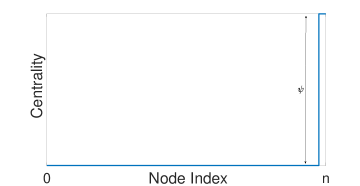
Figure 1: Example of an ideal centrality ranking. The majority of the nodes have a low ranking, and a small $10\%$ minority have a high ranking. The gap separating the low ranked nodes and the high ranked nodes is $\psi$.

Consider the centrality ranking shown in Figure 1. Here we have a situation that is nearly optimal for centrality ranking algorithms. We have a small percentage of nodes that are very important, and a vast majority of nodes that are not important at all. The important nodes are separated from the unimportant nodes by a gap of $\psi$. Given the upper bounds for local sensitivity we have previously computed, we show that we will missclassify all the nodes with high probability, unless the gap $\psi$ is unrealistically large. Since in practice the distribution of node centrality will be much less optimally distributed, this means that after adding noise calibrated to smooth sensitivity we will, in general, preserve no to little utility.

In order to enforce privacy, we need to add a noise vector consisting of $n$ random variables from the Laplace distribution $L(0,b)$, where $b$ is the bound we previously computed for the local sensitivity. This means that our distribution has a variance of $2b^{2}$, and a mean $0$.

Theorem 4.3.

In order for a diferentially private version of eigenvector centrality to correctly classify all but a constant number of nodes $c$, the gap $\psi$ between the important and unimportant nodes must be $O(\sqrt{n})$.

Proof.

In order to misclassify an unimportant node as an important node, we must add noise proportional to the gap $\psi$. We are computing the noise as a vector of $n$ i.i.d random variables drawn from a Laplace distribution $L(0,b)$, where $b=\frac{\sqrt{n}|\theta|}{\delta(A)}$, where $\delta(A)$ is the spectral gap of $A$. Since we are working with the Laplace distribution we can use the cumulative distribution function $1-F(x)=1-(1-\frac{e^{-x/b}}{2}),x\geq 0$ to compute the probability that an element of our noise vector is greater than $\psi$. Then, $n$ times this probability will be the number of misclassified vertices. We wish to compute the minimum size so that the number of misclassified vertices is less than some constant amount $c$. We thus have

$$(1-P(\psi))n<c$$ (6)

$$(1-(1-\frac{e^{-\frac{\psi\delta(A)}{\sqrt{(}n)|\theta|}}}{2}))n<c$$

$$(e^{-\frac{\psi\delta(A)}{\sqrt{(}n)|\theta|}}))n<2c$$

$$(e^{-\frac{\psi\delta(A)}{\sqrt{(}n)|\theta|}})<\frac{2c}{n}$$

$$-\frac{\psi\delta(A)}{\sqrt{(}n)|\theta|}<\log(\frac{2c}{n})$$

$$-\psi<\frac{\log(\frac{2c}{n})\sqrt{n}|\theta|}{\delta(A)}$$

$$\psi>\frac{-\log(\frac{2c}{n})\sqrt{n}|\theta|}{\delta(A)}=O(\sqrt{n})$$

∎

A gap of $O(\sqrt{(}n))$ is grossly unrealistic even for graphs that have an extremely favourable centrality ranking. Since the bounds on local sensitivity for eigenvector centrality are tight for some graphs, in the worst case we cannot offer any computational utility after adding noise. We leave open the question of what the average case is for local sensitivity. However, since local sensitivity serves as a lower bound on smooth sensitivity, it seems likely that in practice the average case is not much better than the worst case. In Section 7 we present empirical results which support this claim.

5 Laplacian centrality

Let $G$ be an undirected and weighted graph with vertices $\{v_{1},\ldots,v_{n}\}$ and weight matrix $W$. The Laplacian matrix of $G$ is defined by $L=X-W$, where $X$ is the diagonal matrix satisfying that $X_{ii}=\sum_{j=1}^{n}W_{ij}$ for every $i\in\{1,\ldots,n\}$.

The Laplace energy of $G$, denoted $\Lambda(G)$, is the sum of the squares of the eigenvalues of the Laplacian matrix of $G$, i.e. $\Lambda(G)=\lambda_{1}^{2}+\cdots+\lambda_{n}^{2}$ where $\lambda_{1},\cdots,\lambda_{n}$ are the eigenvalues of $G$. Considering $G_{v_{i}}$ to be the graph resulting from removing $v_{i}$ from $G$, the Laplacian centrality vector of a graph $G$ is the vector $C_{\mathcal{L}}^{n}(G)=(c_{1},\ldots,c_{n})$ where,

$$c_{i}=\frac{\Lambda(G)-\Lambda(G_{i})}{\Lambda(G)}\ \forall i\in\{1,\ldots,n\}\text{.}$$

We wish to bound $LS_{C_{\mathcal{L}}^{n}}^{\sim}(G)=\|C_{\mathcal{L}}^{n}(G)-C_{\mathcal{L}}^{n}(G^{\prime})\|$ , and then use this to bound $S^{*}_{C_{\mathcal{L}}^{n},\beta}$. We will make use of two well known theorems. The first is Weyl interlacing inequality theorem [24]. This theorem states that given two Hermitian matrices $A$, with eigenvalues $\lambda_{i}$, and a Hermitian perturbation matrix $P$, one can define a new matrix $M=A+P$, and bound its eigenvalues. In particular, the eigenvalues $\mu_{i}$ of M are bounded by $|\mu_{i}-\lambda_{i}|\leq\|P\|$. Here the norm may be any consistent matrix norm, so we consider the $\|P\|_{\infty}$ norm. We note that if we make $k$ changes of size $\theta$ to $G$, then $\|P\|_{\infty}=k\theta$.

We will also make use of a theorem from [15], which states that for an unweighted graph the eigenvalues of a graph created by deleting a vertex $v_{i}$ are bounded as $\lambda_{i}-1\leq\lambda_{i}^{v}\leq\lambda_{i+1}$, where $\lambda_{i}^{v}$ are the eigenvalues of the new graph Laplacian, and $\lambda$ are the eigenvalues of the original graph. We begin by extending this theorem to weighted graphs. In doing so we follow the same argument as the original theorem.

Theorem 5.1.

Let $L$ be the Laplacian of a undirected, weighted graph, with maximum weighted edge $\delta$. Let $L^{v}$ be the graph created by deleting an edge. Let $P$ be the principal sub-matrix of $L$, created by deleting a row and column of $L$. Let the eigenvalues of $L$ be $\lambda_{n}...\geq\lambda_{i}...\geq\lambda_{1}$. Let the eigenvalues of $L^{v}$ be $\lambda^{v}_{n}...\geq\lambda^{v}_{i}...\geq\lambda^{v}_{i}$. Finally let the eigenvalues of $P$ be $\rho_{n}...\geq\rho_{i}...\geq\rho_{1}$. Then we have $\lambda_{i}-\delta\leq\lambda_{i}^{v}$.

Proof.

Since our graph is undirected, we have that $L$ is a symmetric matrix, therefore by the Cauchy interlacing theorem, we have that $\lambda_{1}\leq\rho_{i}..\leq\rho_{n-1}\leq\lambda_{n}$. We now show that $\rho_{i}\leq\lambda^{v}_{i}+\delta$. Define $L_{v}=P-L^{v}$. $I_{v}$ is a diagonal matrix wiht all zero entries except for the $j$-th diagonal entry, which is at most $\delta$, iff $j$ is conected to $v$ in $G$, with weight $\delta$. We iterate over $\forall i\in{1,...,n-1}$. By the Courant-Fischer Theorem [15] we have

$$\rho_{n-i+1}=\max_{U}\min_{x\in U}{\frac{x^{t}Px}{x^{t}x}:U\subseteq\mathbb{R}^{n},\dim(U)=i,x\in U=span(U)}$$ (7)

$$\rho_{n-i+1}=\max_{U}\min_{x\in U}{\frac{x^{t}(L^{v}+I_{v})x}{x^{t}x}:U\subseteq\mathbb{R}^{n},\dim(U)=i,x\in U=span(U)}$$

$$\rho_{n-i+1}\leq\max_{U}\min_{x\in U}{\frac{x^{t}(L^{v})x}{x^{t}x}:U\subseteq\mathbb{R}^{n},\dim(U)=i,x\in U=span(U)}+$$

$$\max_{U}\min_{x\in U}{\frac{x^{t}(I_{v})x}{x^{t}x}:U\subseteq\mathbb{R}^{n},\dim(U)=i,x\in U=span(U)}$$

$$\leq\lambda^{v}_{n-i+1}+\delta$$

We already have that $\lambda_{1}\leq\rho_{i}..\leq\rho_{n-1}\leq\lambda_{n}$. Substitute $\rho_{n-i+1}\leq\lambda^{v}_{n-i+1}+\delta$ and we are left with $\lambda_{i}\leq\lambda^{v}_{i}+\delta$, implying $\lambda_{i}-\delta\leq\lambda^{v}_{i}$.

∎

Theorem 5.2.

Let $G$ be a weighted graph with Laplacian $L$, eigenvalues $\lambda_{n}...\geq\lambda_{i}...\geq\lambda_{1}$, and max weight $\delta$. Let $L^{v}$ be the Laplacian of the graph created by deleting some vertex $v$ from $G$, with eigenvalues $\lambda^{v}_{n}...\geq\lambda^{v}_{i}...\geq\lambda^{v}_{1}$. We have that $LS_{C_{\mathcal{L}}^{n}}^{\sim}(G)=\|C_{\mathcal{L}}^{n}(G)-C_{\mathcal{L}}^{n}(G^{\prime})\|\leq n\sum^{n}_{i=0}2(\lambda_{i}\delta)-\delta^{2}$.

Proof.

We have $c_{i}=\sum^{n}_{i=0}\lambda_{i}^{2}-\sum^{n}_{i=0}\lambda^{v2}_{i}$. By Theorem 5.1 we have that $\lambda^{v}_{i}\leq\lambda_{i-1}-\delta$, so $c_{i}\leq\sum^{n}_{i=0}\lambda_{i}^{2}-\sum^{n}_{i=0}(\lambda_{i}-\delta)^{2}=\sum^{n}_{i=0}(2(\lambda_{i}\delta)-\delta^{2})$. Therefore $\|C_{n}^{e}(G)-C_{n}^{e}(G^{\prime})\|\leq n\sum^{n}_{i=0}(2(\lambda_{i}\delta)-\delta^{2})$. ∎

We now need to bound $S^{*}_{C_{\mathcal{L}}^{n},\beta}$. This reduces to an optimization problem.

Theorem 5.3.

Let $G$ be a weighted graph with Laplacian $L$, eigenvalues $\lambda_{n}...\geq\lambda_{i}...\geq\lambda_{1}$, and max weight $\delta$. Let $L^{v}$ be the Laplacian of the graph created by deleting some vertex $v$ from $G$, with eigenvalues $\lambda^{v}_{n}...\geq\lambda^{v}_{i}...\geq\lambda^{v}_{1}$. We have that $S^{*}_{C_{\mathcal{L}}^{n},\beta}(G)=\max_{G^{\prime}\in D^{n}}\left(LS_{C_{\mathcal{L}}^{n}}^{\sim}(G^{\prime})\cdot e^{-\beta d(G,G^{\prime})}\right)=\|C_{\mathcal{L}}^{n}(G)-C_{\mathcal{L}}^{n}(G^{\prime})\|e^{-\beta\theta}\leq n\sum^{n}_{i=0}(2((\lambda_{i}+\theta)\delta)-\delta^{2})e^{-\beta\theta}$.

Proof.

We know by Wely’s theorem [24] that any perturbation $P$ of the original graph $G$, will perturb the eigenvalues of the Laplacian $L$ of $G$ at most $\|P\|$. If we take the worst case where the perturbation is tight then we have the bound above. If the perturbation is not tight, than the maximum will be reached at a higher $\theta$, and will thus be smaller. ∎

For a given value of $\beta$ we can obtain the worst case $\theta$ by differentiating $n\sum^{n}_{i=0}(2((\lambda_{i}+\theta)\delta)-\delta^{2})e^{-\beta\theta}=0$, with respect to $\theta$, then solving for $\theta$. Unfortunately, it can be seen that these bounds are likely to be very loose in practice, given their dependence on $n$, and the sum of the entire spectrum. Experimentally, we find that using these bounds to generate noise destroys all the information about the node ordering that we were seeking to preserve (see Section 7).

6 Closeness centrality

Closeness centrality measures how well-connected a user is in a social network. Intuitively, the smaller the sum of the weights along a path between vertices $u$ and $v$, the better connected they are. It is worth noting that in this interpretation of connectivity the weights represent the cost of traversing an edge. We use $paths_{G}(u,v)$ to denote the set of all paths between $u$ and $v$ in a graph $G$. The connectivity score between $u$ and $v$ in $G$, denoted $S_{G}(u,v)$, is thus defined by

$$S_{G}(u,v)=\begin{cases}\infty&\text{if $paths_{G}(u,v)=\emptyset$}\\ \min_{(x_{1},\ldots,x_{n})\in paths(u,v)}\sum_{i=1}^{n-1}W(x_{i},x_{i+1})&\text{otherwise}\end{cases}$$

Note that a connectivity score is strictly larger than zero, while it could be $\infty$ if the graph is disconnected. To express the intuition that a low connectivity score makes a vertex more accessible, the closeness centrality score of a vertex $u$ in a graph $G$, denoted $c\mathchar 45\relax score_{G}(u)$, is defined by

$$c\mathchar 45\relax score_{G}(u)=\frac{1}{\sum_{v\in V}S_{G}(u,v)}$$

where, by convention, we take $1/\infty=0$.

We use $C^{c}_{n}$ to denote the closeness centrality function with domain $\mathcal{G}_{n}$ and co-domain $\mathbb{R}^{n}$ defined, for every graph $G$ with totally ordered set of vertices $v_{1}<\cdots<v_{n}$, by

$$C^{c}_{n}(G)=(c\mathchar 45\relax score_{G}(v_{1}),c\mathchar 45\relax score_{G}(v_{2}),\ldots,c\mathchar 45\relax score_{G}(v_{n})).$$

Theorem 6.1.

Let $G=(V,E,W)$ be a graph with $|V|=n$. The local sensitivity of $G$ with respect to the $\theta$-edge neighbouring relation $\sim$ and the closeness centrality measure $C^{c}_{n}$ is upper-bounded by

$$\frac{n\times(n-1)\times\theta}{\sum_{e\in E}W(e)\times(\sum_{e\in E}W(e)-\theta)}.$$

Proof.

Let $G^{\prime}$ be a graph such that $G\sim G^{\prime}$, with $G=(V,E,W)$ and $G^{\prime}=(V,E,W^{\prime})$. Consider two vertices $u,v\in V$, and let the vertex sequence $x_{1},x_{2},\ldots,$ $x_{p}$ with $u=x_{1}$ and $v=x_{p}$ be a shortest $uv$-path in $G$. Similarly, let $x_{1}^{\prime},x_{2}^{\prime},\ldots,x_{q}^{\prime}$ with $u=x_{1}^{\prime}$ and $v=x_{p}^{\prime}$ be a shortest $uv$-path in $G^{\prime}$. It follows that

$$S_{G^{\prime}}(u,v)=\sum_{i=1}^{q-1}W^{\prime}(x_{i}^{\prime},x_{i+1}^{\prime})\leq\sum_{i=1}^{p-1}W^{\prime}(x_{i},x_{i+1}).$$

This means that

$$S_{G^{\prime}}(u,v)-S_{G}(u,v)\leq\sum_{i=1}^{p-1}W^{\prime}(x_{i},x_{i+1})-\sum_{i=1}^{p-1}W(x_{i},x_{i+1}).$$

Now, because $G\sim G^{\prime}$, we obtain that

$$\left|\sum_{i=1}^{p-1}W^{\prime}(x_{i},x_{i+1})-\sum_{i=1}^{p-1}W(x_{i},x_{i+1})\right|\leq\theta,$$

as the weight of at most one edge is different, up to a maximum difference of $\theta$, and by definition a shortest path does not go through the same edge twice. Hence $|S_{G}^{\prime}(u,v)-S_{G}(u,v)|\leq\theta$ This gives the following bound:

$$\sum_{v\in V}|S_{G}^{\prime}(u,v)-S_{G}(u,v)|\leq(n-1)\times\theta.$$

By the triangle inequality, we also obtain

$$\left|\sum_{v\in V}S_{G^{\prime}}(u)-\sum_{v\in V}S_{G}(u)\right|\leq\sum_{v\in V}|S_{G^{\prime}}(u,v)-S_{G}(u,v)|\leq(n-1)\times\theta.$$

The following sequence of algebraic development is useful to bound $\|C_{n}^{C}(G)-C_{n}^{C}(G^{\prime})\|_{1}$:

$$\|C_{n}^{C}(G)-C_{n}^{C}(G^{\prime})\|_{1}=\sum_{u\in V}\left|c\mathchar 45\relax score_{G}(u)-c\mathchar 45\relax score_{G^{\prime}}(u)\right|=$$

$$\sum_{u\in V}\left|\frac{1}{S_{G}(u)}-\frac{1}{S_{G^{\prime}}(u)}\right|=\sum_{u\in V}\frac{\left|S_{G^{\prime}}(u)-S_{G}(u)\right|}{S_{G^{\prime}}(u)\times S_{G}(u)}\leq\sum_{u\in V}\frac{(n-1)\times\theta}{S_{G^{\prime}}(u)\times S_{G}(u)}.$$

Now, we use the fact that $S_{G}(u)\geq\sum_{e\in E}W(e)$ and $S_{G^{\prime}}(u)\geq\sum_{e\in E}W^{\prime}(e)$ to obtain

$$\|C_{n}^{c}(G)-C_{n}^{c}(G^{\prime})\|_{1}\leq\frac{n\times(n-1)\times\theta}{\sum_{e\in E}W^{\prime}(e)\times\sum_{e\in E}W(e)}.$$

Finally, the result follows from the fact that

$$\sum_{e\in E}W^{\prime}(e)\geq\sum_{e\in E}W(e)-\theta.$$

∎

It is worth remarking that the bound above is tight, as the equality holds for any complete graph of order two such that the weight of its sole edge is greater than $\theta$. We now turn to determining the bounds on smooth sensitivity.

Theorem 6.2.

Let $G$ be a graph in $\mathcal{G}_{n}$, $w$ the sum of its weights, and $\sim_{e_{\theta}}$ the $\theta$-edge neighbouring relation with $\theta>0$. For every positive real $\beta$, it holds that

$$S^{*}_{C^{c}_{n},\beta}(G)\leq\max_{k\in\mathbb{N^{+}}}\left(\frac{n\times(n-1)\times\theta}{\left(w-k\theta\right)\times(w-k\theta-\theta)}\cdot e^{-\beta k}\right)$$

Proof.

Take a graph $G^{\prime}$ whose distance to $G$ with respect to $\sim_{e_{\theta}}$ is $k$. It follows that, if $G=(V,E,W)$, then $G^{\prime}=(V,E,W^{\prime})$ for some weight function $W^{\prime}\neq W$. From Theorem 6.1 we obtain that

$$LS_{C_{n}^{c}}^{\sim_{e_{\theta}}}(G^{\prime})\leq\frac{n\times(n-1)\times\theta}{\sum_{e\in E}W^{\prime}(e)\times(\sum_{e\in E}W^{\prime}(e)-\theta)}.$$ (8)

Now, recall from Definition 3.3 that $d(G,G^{\prime})=k$ means that $k$ is the smallest positive integer such that there exists $G_{0},\ldots,G_{k}\in\mathcal{G}$ such that $G_{0}=G$, $G_{k}=G^{\prime}$ and $G_{0}\sim_{e_{\theta}}\cdots\sim_{e_{\theta}}G_{k}$. Therefore, it follows that $\sum_{e\in E}W(e)-k\theta\leq\sum_{e\in E}W^{\prime}(e)$. By substituting in Equation 8 we obtain that, if $\sum_{e\in E}W(e)-k\theta-\theta>0$, then,

$$LS_{C_{n}^{c}}^{\sim_{e_{\theta}}}(G^{\prime})\leq\frac{n\times(n-1)\times\theta}{\left(\sum_{e\in E}W(e)-k\theta\right)\times(\sum_{e\in E}W(e)-k\theta-\theta)}.$$

The proof is completed by using the inequality above and the definition of smooth sensitivity. ∎

Theorem 6.2 serves as the basis of an algorithmic approach to calculate a bound for smooth sensitivity, which is depicted in Algorithm 1.

Algorithm 1 Given a graph $G$ of order $n$, and real values $\theta$, $\varepsilon$ and $\beta$, outputs a randomised algorithm that satisfies $\left(\varepsilon,\frac{1}{e^{\frac{\varepsilon}{\sqrt{n}\beta}}}\right)$-differential privacy, if it exists.

1:Let $w$ be the sum of the edge weights in $G$ with $w>\theta$

2:Let $f(x)=\frac{n\times(n-1)\times\theta}{\left(w-x\theta\right)\times(w-x\theta-\theta)}\cdot e^{-\beta x}$

3:Let $k=0$

4:while $f(k)<f(k+1)$ do

5:     if $w-k\theta-\theta\leq 0$ then

6:         return Smooth sensitivity is undefined within $\mathbb{N}$.

7:     end if

8:     $k=k+1$

9:end while

10:Let $\alpha=\frac{\varepsilon}{2}$

11:Let $Z$ be random variable sampled according to $h(z)=\frac{1}{2}\cdot e^{-|z|_{1}}$.

12:return Algorithm $\mathcal{A}(x)=C^{c}_{n}(x)+\frac{f(k)}{\alpha}\cdot Z$ is $\left(\varepsilon,\frac{1}{e^{\frac{\varepsilon}{\sqrt{n}\beta}}}\right)$-differentially private.

Correctness of the algorithm above follows from Lemma 2.5, Example 3 in [18] and the claim that the function $f(k)=\frac{n\times(n-1)\times\theta}{\left(w-k\theta\right)\times(w-k\theta-\theta)}\cdot e^{-\beta k}$ has a single maximum within the natural numbers domain.

7 Empirical analysis

Here we compare the effect on utility of adding noise calibrated to the exact value of local sensitivity, the bounds on local sensitivity enunciated above, and the smooth sensitivity (where possible) for a collection of real-life and synthetic social graphs. The results confirm our theoretical results that the noise needed to provide $(\varepsilon,\delta)$-differential privacy has the potential to severely affect utility.

The graphs we have selected are SNAP/p2p-Gnutella05, Wiki-Vote, a synthetic preferential attachment graph, and a synthetic small world graph, created using the Matlab CONTEST toolbox, using $\mathcal{O}(10^{4})$ nodes and the default attachment settings. We generate these graphs one time, and then reuse them throughout our experiments, while the real-life social network graphs can be obtained from the SuiteSparse Matrix Collection [4]. For each graph, we computed the real rankings for the most important $5$, $10$ and $15$ percent of the nodes, and compare this to the differentially private rankings in order to compute the precision of our method. For our experiments, we used $\varepsilon=2$ and a value of $\theta$ equal to the maximum edge weight of the graph under analysis. Certainly, those values are the edge of the maximum privacy that can be offered via differential-privacy, yet they are plausible values for a practical setting. We leave for future work the full analysis of the privacy-utility trade-off over the entire domains of $\varepsilon$ and $\theta$.

	Local Sensitivity			B. L. Sensitivity			B. S. Sensitivity
	5%	10%	15%	5%	10%	15%	5%	10%	15%
p2p-Gnutella05	$9$	$13$	$18$	$5$	$9$	$15$	N/A
Wiki-Vote	$72$	$67$	$65$	$6$	$11$	$15$	N/A
Synt. Pref. Attach.	$5$	$9$	$14$	$6$	$10$	$15$	N/A
Synt. Small World	$4$	$10$	$13$	$5$	$10$	$15$	N/A

Table 1: Precision values, in percentages, for eigenvector centrality at the top $5\%$, $10\%$ and $15\%$ of the rankings. Since we have no mechanism to calculate or effectively bound smooth sensitivity, the corresponding columns of the table are empty.

We begin our analysis by computing the percentage of correctly identified nodes in the top $5/10/15$ percent of the nodes in the perturbed graph using eigenvector centrality. The results are displayed in Table 1. They show that very few of the important nodes are preserved after perturbation. Although the noise added to the Wiki-Vote graph based on the local sensitivity parameter does not completely destroy the rankings, the precision quickly degrades when using the bound of the local sensitivity. The precision on the other graphs under consideration does not significantly differ from random noise.

In Table 2 we display the experimental results for closeness centrality. In this case, even for local sensitivity, the outputs are dominated by random noise.

	Local Sensitivity			B. L. Sensitivity			B. S. Sensitivity
	5%	10%	15%	5%	10%	15%	5%	10%	15%
p2p-Gnutella05	$5$	$8$	$15$	$4$	$9$	$14$	$4$	$9$	$4$
Wiki-Vote	$5$	$8$	$15$	$3$	$9$	$14$	$3$	$9$	$14$
Synt. Pref. Attach.	$4.5$	$11$	$15$	$3.5$	$10$	$16$	$3.5$	$10$	$16$
Synt. Small World	$5$	$10$	$13$	$5$	$8$	$15$	$5$	$8$	$15$

Table 2: Precision values, in percentages, for closeness centrality at the top $5\%$, $10\%$ and $15\%$ of the rankings.

Finally, we examine the results for Laplacian centrality in Table 3. Unlike eigenvector and closeness centralities, Laplacian centrality does preserve a statistically significant number of the original nodes in the original ranking when applying noise proportional to local sensitivity. Unfortunately, because the bounds on local and smooth sensitivity for this measure are very loose, we are not able to achieve an accurate differentially private computation in practice.

	Local Sensitivity			B. L. Sensitivity			B. S. Sensitivity
	5%	10%	15%	5%	10%	15%	5%	10%	15%
p2p-Gnutella05	$34$	$36$	$38$	$6$	$10$	$15$	$6$	$10$	$15$
Wiki-Vote	$91$	$81$	$81$	$6$	$9$	$16$	$6$	$9$	$16$
Synt. Pref. Attach.	$89$	$94$	$90$	$5$	$9$	$15$	$5$	$9$	$15$
Synt. Small World	$8$	$13$	$21$	$5$	$10$	$15$	$5$	$10$	$15$

Table 3: Precision values, in percentages, for Laplacian centrality at the top $5\%$, $10\%$ and $15\%$ of the rankings.

8 Conclusions

We have presented the first analysis of the differentially private computation of non trivial centrality measures on weighted graphs. Our study covered eigenvector, Laplacian and closeness centralities. We presented lower and upper bounds on the amount of noise that randomised algorithms based on the smooth sensitivity approach need to add in order to make the output of each measure differentially private. Our results entail that differentially private computation of the three centrality measures via the smooth sensitivity approach is either infeasible, in the sense that there are large families of graphs for which smooth sensitivity is unbounded; or impractical, in the sense that even for the cases where smooth sensitivity is bounded, the required amounts of noise result in unacceptably large utility losses in terms of the quality of centrality-based node rankings.

Acknowledgements. The work of Yunior Ramírez-Cruz was funded by Luxembourg’s Fonds National de la Recherche (FNR), grant C17/IS/11685812 (PrivDA). Part of this article was written while Yunior Ramírez-Cruz was visiting the School of Information Technology at Deakin University.

References

- [1] Xihui Chen, Sjouke Mauw, and Yunior Ramírez-Cruz. Publishing community-preserving attributed social graphs with a differential privacy guarantee. Proccedings on Privacy Enhancing Technologies, 2020(4):131–152, 2020.
- [2] Aaron Clauset, Cristopher Moore, and M. E. J. Newman. Hierarchical structure and the prediction of missing links in networks. Nature, 453:98–101, 2008.
- [3] Chandler Davis and W. M. Kahan. Some new bounds on perturbation of subspaces. Bull. Am. Math. Soc, 75(4):863–868, 1969.
- [4] Timothy A. Davis and Yifan Hu. The university of florida sparse matrix collection. ACM Trans. Math. Softw., 38(1), December 2011.
- [5] Cynthia Dwork. Differential privacy. In Michele Bugliesi, Bart Preneel, Vladimiro Sassone, and Ingo Wegener, editors, Automata, Languages and Programming, pages 1–12, Berlin, Heidelberg, 2006. Springer Berlin Heidelberg.
- [6] Cynthia Dwork and Aaron Roth. The algorithmic foundations of differential privacy. Foundations and Trends® in Theoretical Computer Science, 9(3–4):211–407, 2014.
- [7] Anupam Gupta, Katrina Ligett, Frank McSherry, Aaron Roth, and Kunal Talwar. Differentially private combinatorial optimization. In Proceedings of the Twenty-first Annual ACM-SIAM Symposium on Discrete Algorithms, SODA ’10, pages 1106–1125, Philadelphia, PA, USA, 2010. Society for Industrial and Applied Mathematics.
- [8] Michael Hay, Chao Li, Gerome Miklau, and David D. Jensen. Accurate estimation of the degree distribution of private networks. In Proc. 19th IEEE International Conference on Data Mining (ICDM), pages 169–178. IEEE Computer Society, 2009.
- [9] Joseph J. Pfeiffer III, Sebastián Moreno, Timothy La Fond, Jennifer Neville, and Brian Gallagher. Attributed graph models: modeling network structure with correlated attributes. In Proc. 23rd International World Wide Web Conference (WWW), pages 831–842. ACM Press, 2014.
- [10] Zach Jorgensen, Ting Yu, and Graham Cormode. Publishing attributed social graphs with formal privacy guarantees. In Proc. 2016 International Conference on Management of Data (SIGMOD), pages 107–122. ACM Press, 2016.
- [11] Mikhail Belkin Justin Eldridge and Yusu Wang. Unperturbed: spectral analysis beyond davis-kahan. Proceedings of Machine Learning Research, 83:321–358, 2018.
- [12] Vishesh Karwa, Sofya Raskhodnikova, Adam D. Smith, and Grigory Yaroslavtsev. Private analysis of graph structure. ACM Transactions on Database Systems, 39(3):22:1–22:33, 2014.
- [13] Vishesh Karwa and Aleksandra B. Slavkovic. Differentially private graphical degree sequences and synthetic graphs. In Proc. 2012 International Conference on Privacy in Statistical Databases (PSD), volume 7556 of Lecture Notes in Computer Science, pages 273–285. Springer, 2012.
- [14] Jure Leskovec and Christos Faloutsos. Scalable modeling of real graphs using kronecker multiplication. In Proc. 24th International Conference on Machine Learning (ICML), pages 497–504. ACM Press, 2007.
- [15] Zvi Lotker. Note on deleting a vertex and weak interlacing of the laplacian spectrum. ELA. The Electronic Journal of Linear Algebra [electronic only], 16, 02 2007.
- [16] Darakhshan J. Mir and Rebecca N. Wright. A differentially private graph estimator. In Proc. 2009 ICDM International Workshop on Privacy Aspects of Data Mining (ICDM), pages 122–129. IEEE Computer Society, 2009.
- [17] Hiep H. Nguyen, Abdessamad Imine, and Michaël Rusinowitch. Detecting communities under differential privacy. In Proc. 2016 ACM Workshop on Privacy in the Electronic Society (WPES), pages 83–93. ACM Press, 2016.
- [18] Kobbi Nissim, Sofya Raskhodnikova, and Adam Smith. Smooth sensitivity and sampling in private data analysis. In Proc. 39th Annual ACM Symposium on Theory of Computing (STOC), pages 75–84. ACM Press, 2007.
- [19] Alessandra Sala, Xiaohan Zhao, Christo Wilson, Haitao Zheng, and Ben Y. Zhao. Sharing graphs using differentially private graph models. In Proc. 11th ACM SIGCOMM Internet Measurement Conference (IMC), pages 81–98. ACM Press, 2011.
- [20] Julián Salas and Vicenç Torra. Differentially private graph publishing and randomized response for collaborative filtering. In Procs. of Secrypt 2020, pages 407–414, 2020.
- [21] Santiago Segarra and Alejandro Ribeiro. Stability and continuity of centrality measures in weighted graphs. IEEE Trans. Signal Processing, 64(3):543–555, 2016.
- [22] Yue Wang and Xintao Wu. Preserving differential privacy in degree-correlation based graph generation. Transactions on Data Privacy, 6(2):127–145, 2013.
- [23] Yue Wang, Xintao Wu, Jun Zhu, and Yang Xiang. On learning cluster coefficient of private networks. Social Network Analysis and Mining, 3(4):925–938, 2013.
- [24] Hermann Weyl. Das asymptotische Verteilungsgesetz der eigenwerte linearer partieller Differentialgleichungen. Mathematische Annalen, 71(4):441 – 479, 1912.
- [25] Qian Xiao, Rui Chen, and Kian-Lee Tan. Differentially private network data release via structural inference. In Proc. 20th ACM SIGKDD International Conference on Knowledge Discovery and Data Mining (KDD), pages 911–920. ACM Press, 2014.
- [26] Jun Zhang, Graham Cormode, Cecilia M. Procopiuc, Divesh Srivastava, and Xiaokui Xiao. Private release of graph statistics using ladder functions. In Proc. 36th ACM International Conference on Management of Data (SIGMOD), pages 731–745. ACM Press, 2015.