Properties of the Center of Gravity as an Algorithm for Position Measurements: Two-Dimensional Geometry

Abstract

The center of gravity as an algorithm for position measurements is analyzed for a two-dimensional geometry. Several mathematical consequences of discretization for various types of detector arrays are extracted. Arrays with rectangular, hexagonal, and triangular detectors are analytically studied, and tools are given to simulate their discretization properties. Special signal distributions free of discretized error are isolated. It is proved that some crosstalk spreads are able to eliminate the center of gravity discretization error for any signal distribution (ideal detectors). Simulations, adapted to the CMS em-calorimeter and to a triangular detector array, are provided for energy and position reconstruction algorithms with a finite number of detectors.

PACS 07.05.Kf; 06.30.Bp; 42.30.Sy

Keywords: Center of Gravity, Centroiding, Position Measurements

1 Introduction 2021

The aim of this paper was the study of the e.m. calorimeters, the pixel detectors were in an early stages and we neglected them. The availability of data on silicon micro-strip detectors deviated our attention from this aim, and from further extension to a three-dimensional spherical geometry. Preliminary steps in this last direction showed error patterns very similar to those in the following, with deep valleys near to exact reconstructions. However, the complexity of the Bessel j-functions suggested an early abandon of the project for the probably lack of readers. Instead, the silicon micro-strips are an ideal one dimension system, perfect for ref. [1]. The deep analysis of those data, evidenced the impossibility of a single variance for each hit (homoscedasticity), as it is usually assumed in track fitting. The study of methods to handle those probabilities absorbed all our attentions and produced very interesting new results. This shift of interests, did not allow applications of the two-dimension COG properties, even if the recent use of the silicon pixel-detectors would be a perfect combination of tracking and positioning. However, the difficulty to access to data hinders this possibility. The complexity of the developments here described requires a mathematical skill not frequent among the experimental staffs. Unfortunately, the reconstruction algorithms are complex mathematical instruments and any data analysis can not avoid those complications. Some printing errors, due to the splitting of the equations in two columns, were corrected. The explicit definition of the ideal detector is introduced also for this two-dimensional geometry, as we did for the one dimension system in arXiv:1908.04447. In successive works, these types of detectors were indicated in this synthetic way, sure of its introduction here and in ref. [1]. Among the beneficial effects of the absence of the discretization errors (ideal detectors), it must be recalled its effectiveness in the noise regularization with a drastic simplification in the handling of the detector heteroscedasticity.

2 Introduction

The center of gravity (COG) is a widespread method of pattern recognition used in experimental works as a tool to improve position reconstruction from sets of measurements. Our previous work [1] was devoted to the introduction of methods to define COG properties when the COG is applied. The approach [1] was limited to one-dimensional systems, and only a marginal attention was devoted to two-dimensional systems, when they can be reverted to two one-dimensional systems. This condition covers only a restricted class of two-dimensional detectors: Array of rectangular detectors with constant efficiency, no loss at the border, the COG algorithm calculated with an infinite row of detectors in one direction. Thus, the dependence of the signal distribution on $y$ does not contribute to the COG calculation in $x$, and the two-dimensional problem is split into two one-dimensional configurations. These limitations could be very unrealistic in a few cases, even for detectors of the indicated type. Detectors of different shapes, hexagonal, triangular etc. can never be reduced to two one-dimensional configurations.

Generalization to a two-dimensional geometry entails additional complications compared to  [1], and many more forms and setups are allowed. In this work, we will limit our considerations to parallelogram, hexagon, and triangle detector arrays. These forms cover almost all the types of detectors used in high-energy physics. Although the triangular forms have not been widely used in recent years, the Crystal Ball detector  [2] has an em-calorimeter with triangular-section crystals. The study of the triangular forms allows us to determine the method to treat far more complex detector arrays.

As will be evident, this work is largely based on the results of  [1], but due to the necessity of a two-dimensional generalization and the special handling required by the hexagons and triangles, almost all the equations will be derived in the new context. Array periodicity is a fundamental tool for our derivations. A group of detectors can easily be approximated with a periodic lattice owing to the finite—generally small—range of the signal distributions that affects a small number of detectors, which can almost always be replicated as a periodic mosaic. For this reason, Section 2 introduces the initial definitions and the general equations that are valid for any type of periodic detector array.

In Section 3, the equations are applied to three types of detector array: Parallelograms, hexagons, and triangles. The triangle array exemplifies the way of handling any type of detector mosaic.

Section 4 is devoted to the study of the signal distributions whose COGs are free of discretization errors. It will be evident that the parallelograms, hexagons, and triangles are an extremely reduced sample of the class of signal distributions that have exact COGs at particular sizes. It is surprising how large this class is compared to the one-dimensional case.

Section 5 deals with the modifications introduced by loss and crosstalk. Loss destroys the splitting of a two-dimensional problem into two one dimensions, even for an array of rectangular detectors. There is a large set of crosstalk functions that saves the norm and spreads the incident signal among the detectors in such a way as to eliminate the COG errors for any type of signal distribution. We will also determine the connection to other mathematical properties far from the COG problems.

In Section 6, array periodicity is abandoned and a method to handle a finite set of detectors is defined. The method is applied to the CMS and Crystal Ball em-calorimeter.

Section 7 concludes and summarizes the results.

3 Sampling in Two Dimensions

3.1 Definition of the Formalism

To introduce some notation, let us consider an array of rectangular detectors as shown in

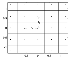
Figure 1: Array of rectangular detectors, $\tau_{1}$ is the $x$-distance of the centers of two neighboring detectors, $\tau_{2}$ is the $y$-distance.

Fig. 1. The two constants $\tau_{1}$ and $\tau_{2}$ establish the size of the array; $\tau_{1}$ is the distance from the center of a detector to the center of its neighbor in $x$-direction, $\tau_{2}$ is the same in $y$-direction. If $\tau_{1}=\tau_{2}$, the detectors have a square section.

As in  [1], we will mainly consider average signal distributions on which we impose some symmetry conditions deriving from the assumed homogeneity of the medium where the signal distribution is produced. These conditions are not essential to our procedures. The equations are able to handle nonsymmetric signal distributions as well, but the asymmetry is rarely experimentally measurable, thereby forcing us to consider averages over asymmetries. Simulation differs in that the asymmetric signal distributions can be easily generated and accounted for. Other implicit conditions are positivity and connectedness of the signal distribution (an em shower in a calorimeter); no limitations of these type will affect the equations, and we will give examples of nonconnected signal distributions.

Let us define $\varphi(\mathbf{x})$ as the signal distribution. As vectorial notation will be used almost everywhere, $\mathbf{x}$ indicates variables $x,y$. We will abandon the vectorial notation when the expressions are not overly long. On $\varphi(\mathbf{x})$, we impose the following two conditions:

$$\int_{\mathbb{R}^{2}}\mathrm{d}\mathbf{x}\ \mathbf{x}\varphi(\mathbf{x})=0,$$ (1)

$$\int_{\mathbb{R}^{2}}\ \mathrm{d}\mathbf{x}\ \varphi(\mathbf{x})=1.$$ (2)

Equation (1) fixes the position of the two COGs $\mathbf{r}_{g}=(x_{g},y_{g})$ of $\varphi(\mathbf{x})$ at the origin of the axes, where as explained in Fig. 1, the COG of a detector is located. It is clear that a symmetric signal distribution $\varphi(\mathbf{x})=\varphi(-\mathbf{x})$ satisfies the two equations. Equation (2) is a normalization condition that eliminates a constant in some of the following procedures.

A good detector generally performs a linear transformation on the collected signal. For example, a good crystal of an em-calorimeter integrates the energy converging on it. The most general linear transformation on the signal distribution induced by a detector is the convolution:

$$\mathrm{f}(\mathbf{x})=\int_{\mathbb{R}^{2}}\mathrm{g}(\mathbf{x}-\mathbf{x}^{\prime})\varphi(\mathbf{x}^{\prime})\,\mathrm{d}\mathbf{x}\ ,$$ (3)

where g$(\mathbf{x})$ embodies the effects of the detector. If $\varphi(\mathbf{x})$ is shifted from the origin by a vector $\boldsymbol{\varepsilon}=(\varepsilon_{1};\varepsilon_{2})$ in $x$-direction and in $y$-direction, f$(\mathbf{x})$ becomes:

$${\mathrm{f}_{\boldsymbol{\varepsilon}}}(\mathbf{x})=\int_{\mathbb{R}^{2}}\mathrm{g}(\mathbf{x}-\mathbf{x}^{\prime})\varphi(\mathbf{x}^{\prime}-\boldsymbol{\varepsilon})\,\mathrm{d}\mathbf{x}^{\prime}\ .$$ (4)

For the properties of the convolution [3] we get:

$$\mathrm{f}_{\boldsymbol{\varepsilon}}(\mathbf{x})=\int_{\mathbb{R}^{2}}\mathrm{g}(\mathbf{x}-\boldsymbol{\varepsilon}-\mathbf{x}^{\prime})\varphi(\mathbf{x}^{\prime})\,\mathrm{d}\mathbf{x}^{\prime}\ ,$$

so f${}_{\boldsymbol{\varepsilon}}(\mathbf{x})$ becomes:

$$\mathrm{f}_{\boldsymbol{\varepsilon}}(\mathbf{x})=\mathrm{f}(\mathbf{x}-\boldsymbol{\varepsilon})\ .$$ (5)

With the normalization of Eq. (2) and assuming Eq. (1) even for g$(\mathbf{x})$, the definition of the COG is proportional to the first moment of f${}_{\boldsymbol{\varepsilon}}(\mathbf{x})$. Convolution theorems [3] state that the first moment of f${}_{\boldsymbol{\varepsilon}}(\mathbf{x})$ is the sum of the first moment of g$(\mathbf{x})$ and the first moment of $\varphi(\mathbf{x}-\boldsymbol{\varepsilon})$. Hence, for our choice of the reference system, the COG of f${}_{\boldsymbol{\varepsilon}}(\mathbf{x})$ is $\boldsymbol{\varepsilon}$. At this level, the linear transformation of Eq. (4) on the signal distribution does not modify the COGs positions.

3.2 Sampling on a Rectangular Lattice

It is evident that Eq. (4) is not the true transformation performed by the detector on the signal. The function f${}_{\boldsymbol{\varepsilon}}(\mathbf{x})$ is not measured for any $\mathbf{x}\in\mathbb{R}^{2}$ nor does the detector continuously "scan" the signal distribution. The measuring device is a set of detectors that are well fixed in definite spatial points, and they give only a sampling of the function f${}_{\boldsymbol{\varepsilon}}(\mathbf{x})$ with very few points above the detector noise. This discretization is the principal source of systematic error of the COG as a position reconstruction algorithm.

The detectors in the array will be considered identical and arranged in a periodic rectangular lattice. To simplify the notations, we shall consider in the following $n,l\in\mathbb{Z}^{2}$, and in absence of other indication our sums will run over $n,l\in\mathbb{Z}^{2}$. We will indicate the constants of the sampling lattice as $\mathbf{d}_{1}=(\tau_{1};0)$ and $\mathbf{d}_{2}=(0;\tau_{2})$. If $\big{\{}$f${}_{\boldsymbol{\varepsilon}}(n\mathbf{d}_{1}+l\mathbf{d}_{2})\big{\}}$ is a set of sampled values extracted from f${}_{\boldsymbol{\varepsilon}}(\mathbf{x})$, the COG $\mathbf{r}_{g}=(x_{g};y_{g})$ of the set is given by (with $x_{g}$ the COG in $x$-direction and $y_{g}$ the COG in $y$-direction):

$$\mathbf{r}_{g}=\sum_{n,l}\ (n\mathbf{d}_{1}+l\mathbf{d}_{2})\mathrm{f}_{\boldsymbol{\varepsilon}}(n\mathbf{d}_{1}+l\mathbf{d}_{2})\ \ \ \ \ \sum_{n,l}\mathrm{f}_{\boldsymbol{\varepsilon}}(n\mathbf{d}_{1}+l\mathbf{d}_{2})=1\ .$$ (6)

Assuming a lossless detector array, the sampling of f${}_{\boldsymbol{\varepsilon}}(\mathbf{x})$ saves the normalization. In the presence of loss, the normalization is no longer saved, and $\mathbf{r}_{g}$ can be recast in the form:

$$\mathbf{r}_{g}(\boldsymbol{\varepsilon})=\boldsymbol{\varepsilon}+\frac{\sum_{n,l}(n\mathbf{d}_{1}+l\mathbf{d}_{2}-\boldsymbol{\varepsilon})\mathrm{f}(n\mathbf{d}_{1}+l\mathbf{d}_{2}-\boldsymbol{\varepsilon})}{\sum_{n,l}\mathrm{f}(n\mathbf{d}_{1}+l\mathbf{d}_{2}-\boldsymbol{\varepsilon})},$$ (7)

where we use Eq. (5) and the difference of $\mathbf{r}_{g}$ (the COG position) with respect to the exact position $\boldsymbol{\varepsilon}$ is isolated. This vectorial notation seems to mix rows of detectors (index $n$) and columns (index $l$) in the equations for $\mathbf{r}_{g}$. The two vectors $\mathbf{d}_{1}$ and $\mathbf{d}_{2}$ are parallel respectively to the $x$ and $y$ axes, and their orthogonality eliminates the mixture. In the following, the nonorthogonal lattices will explicitly require such mixture.

The modifications of Eq. (7) to deal with a subset of detectors are straightforward. The sum on $n$ and $l$ must cover only the detectors considered. More developments are required to highlight the dependence on the system parameters, i.e., detector efficiency and shape and signal distribution and position.

Let us prove further properties of Eqs. (6). In [1], we studied a general efficiency function g$(x)$ that could be different from zero even for values of $x$ outside the space of a single detector (crosstalk). We called uniform crosstalk the efficiency functions g$(x)$ having almost everywhere (a. e.) the property $\Sigma_{n}$g$(n\tau-x)=1$. The definition is extended for a two-dimensional system (here and in the following g$(\mathbf{x})$ is normalized as a detector of unitary efficiency and area $\tau_{1}\tau_{2}$) :

$$\sum_{n,l}\mathrm{g}(n\mathbf{d}_{1}+l\mathbf{d}_{2}-\mathbf{x})=1\ \ \ \ \mathit{(a.e.).}$$ (8)

The condition of validity for Eq. (8) a. e. means that in a null set (for example, at the detector boundaries) violations are allowed. These violations have no effect on Eq. (6) due to the convolution operation on the function g$(\mathbf{x})$ that eliminates all them. The notation of Eq. (8) generalizes the intuition of an infinite array of identical detectors each with unitary efficiency packed without holes and area $\tau_{1}\tau_{2}$. Evidently, Eq. (8) deals with more complex configurations than this naive intuition: It automatically contains the crosstalk that distributes part of the signal collected by a detector to nearby ones. It is easy to prove the normalization conservation in the presence of uniform crosstalk:

$$\sum_{n,l}\mathrm{f}(n\mathbf{d}_{1}+l\mathbf{d}_{2}-\boldsymbol{\varepsilon})=\int_{\mathbb{R}^{2}}\big{[}\sum_{n,l}\mathrm{g}(n\mathbf{d}_{1}+l\mathbf{d}_{2}-\boldsymbol{\varepsilon}-\mathbf{x}^{\prime})\big{]}\varphi(\mathbf{x}^{\prime})\,\mathrm{d}\mathbf{x}^{\prime}\ ,$$

and, applying Eq. (8) in parentheses, the right-hand side becomes the normalization of $\varphi(\mathbf{x})$. The condition for the absence of discretization error in $\mathbf{r}_{g}$ can be extracted similarly from Eq. (7):

$$\mathbf{r}_{g}=\boldsymbol{\varepsilon+}\sum_{n,l}(n\mathbf{d}_{1}+l\mathbf{d}_{2}-\boldsymbol{\varepsilon})\mathrm{f}(n\mathbf{d}_{1}+l\mathbf{d}_{2}-\boldsymbol{\varepsilon})$$

$$\mathbf{r}_{g}=\boldsymbol{\varepsilon}+\int_{\mathbb{R}^{2}}\big{[}\sum_{n,l}(n\mathbf{d}_{1}+l\mathbf{d}_{2}-\boldsymbol{\varepsilon}-\mathbf{x}^{\prime})\ \mathrm{g}(n\mathbf{d}_{1}+l\mathbf{d}_{2}-\boldsymbol{\varepsilon}-\mathbf{x}^{\prime})\big{]}\varphi(\mathbf{x}^{\prime})\,\mathrm{d}\mathbf{x}^{\prime}\ .$$

The $-\mathbf{x}^{\prime}$ term introduced in the parentheses gives no contribution to the integral due to Eqs. (8,1). Therefore, the condition for the absence of discretization error in $\mathbf{r}_{g}$ for any signal distribution is given by:

$$\sum_{n,l}(n\mathbf{d}_{1}+l\mathbf{d}_{2}-\mathbf{x})\ \mathrm{g}(n\mathbf{d}_{1}+l\mathbf{d}_{2}-\mathbf{x})=0\ \ \ \mathit{(a.e.)}\ .$$ (9)

In the following, we will show how to construct g-functions with the property of Eq. (9).

3.3 Sampling on a Parallelogram Lattice

To handle more complex, albeit periodic, detector arrays, we have to abandon the simple symmetry of the rectangular array of sampling points and move

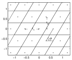
Figure 2: Array of parallelogram detectors: $\tau_{1}$ is the $x$-distance of the centers of two neighboring detectors, $\tau_{2}$ is the $y$-distance, $\theta$ is the bending angle of the inclined sides.

on to a more general set of samples organized as an array of parallelograms (anomalous torus), as given in Fig. 2. On $x$, the family of sampling points is given by horizontal straight-lines; on $y$, the family of sampling points is given by the straight-lines at an angle $\vartheta$ with the horizontal. Our reference system is oriented to have this setup; if rotations are present, these are charged to the signal distributions. As above, $\tau_{1}$ is the distance of the two consecutive detector centers in direction $x$, and $\tau_{2}$ is the distance of two consecutive detector centers in direction $y$, $\alpha=\tan(\theta)$ is the angular coefficient of the inclined lines. At first glance, this array of sampling points suggests parallelogram detector forms, where the rectangular array is given by $\alpha\rightarrow\infty$. In reality, many detector forms are allowed, and the arrays of hexagonal and triangular detectors can be sampled as in Fig. 2. This type of symmetry is connected to the periodic plane tessellation.

We will not even attempt to list all the detector arrays which are covered by a sampling along the vertices of a parallelogram. For example, all plane tessellation images by Escher [4] are created by pictures that can be sampled along two families of parallel straight lines, whereas the Penrose tiles [5] are not. Fortunately, no use of these forms is forecast in real detectors. Theoretically, the equations we are developing can handle the exotic forms of Ref. [4] and a subset of the Penrose tiles.

Neglecting the detector form complications on sampling schema, the linear effect of a single detector on $\varphi(\mathbf{x})$ is always contained in Eq. (3). The sampled version of Eq. (3) has a few differences. Formally, the sampling is generated by multiplying continuous functions with sums of Dirac $\delta$-functions that record the sampling points [6]. In a periodic array, the $\alpha$ value is not univocally defined. We can define $\alpha$ with any detector in the upper line (Fig. 2), then $\alpha_{\rho}^{-1}=\alpha_{0}^{-1}+\rho\tau_{1}/\tau_{2}$ where $\rho\in\mathbb{Z}$, and $\alpha_{0}^{-1}$ is the minimum of the positive values of $\alpha_{\rho}^{-1}$ . Any other $\alpha_{\rho}$ simply relabels the detectors. To avoid ambiguities, we will always use $\alpha=\alpha_{0}$. Now the lattice constants are $\mathbf{n}_{1}=(\tau_{1},\ 0)$ and $\mathbf{n}_{2}=(\tau_{2}/\alpha,\ \tau_{2})$. The vector $\mathbf{n}_{2}$ is no longer parallel to the $y$-axis and introduces a mixture of $n$ and $l$ sums. The vectorial notation hides this difference with respect to the orthogonal sampling, but it is fundamental in the applications.

If s${}_{\boldsymbol{\varepsilon}}(\mathbf{x})$ is the result of the sampling operating on f${}_{\boldsymbol{\varepsilon}}(\mathbf{x})$, it can be expressed as:

$$\mathrm{s}_{\boldsymbol{\varepsilon}}(\mathbf{x})=\sum_{n,l}\delta(\mathbf{x}-n\mathbf{n}_{1}-l\mathbf{n}_{2})\ \mathrm{f}(n\mathbf{n}_{1}+l\mathbf{n}_{2}-\boldsymbol{\varepsilon}),$$ (10)

its Fourier Transform (FT) is defined as usual ($\boldsymbol{\omega}=(\omega_{x},\ \omega_{y})$):

$$\mathrm{S}_{\boldsymbol{\varepsilon}}(\boldsymbol{\omega})=\int_{\mathbb{R}^{2}}\mathrm{e}^{-i{\boldsymbol{\omega}}\cdot\mathbf{x}}\mathrm{s}_{\boldsymbol{\varepsilon}}(\mathbf{x})\ \mathrm{d}\mathbf{x}$$

or, using Eq. (10), $\mathrm{S}_{\boldsymbol{\varepsilon}}(\boldsymbol{\omega})$ becomes:

$$\mathrm{S}_{\boldsymbol{\varepsilon}}(\boldsymbol{\omega})=\sum_{n,l}\mathrm{e}^{-i\boldsymbol{\omega}\cdot(n\mathbf{n}_{1}+l\mathbf{n}_{2})}\>\mathrm{f}\,(n\mathbf{n}_{1}+l\mathbf{n}_{2}-\boldsymbol{\varepsilon}).$$ (11)

Now $\mathbf{r}_{g}$ can be defined through $\mathrm{S}_{\boldsymbol{\varepsilon}}(\boldsymbol{\omega})$ with:

$$\mathbf{r}_{g}=\frac{i}{\mathrm{S}_{\boldsymbol{\varepsilon}}(0)}\boldsymbol{\nabla}_{\boldsymbol{\omega}}\,\mathrm{S}_{\boldsymbol{\varepsilon}}(\boldsymbol{\omega})\Big{|}_{\boldsymbol{\omega}\rightarrow 0}\ .$$ (12)

If the normalization of $\varphi(\mathbf{x})$ is conserved (i.e., all the energy released in a calorimeter is collected), $\mathrm{S}_{\boldsymbol{\varepsilon}}(0)$ is equal to one, and Eq. (11) yields:

$$\mathrm{S}_{\boldsymbol{\varepsilon}}(0)=\sum_{n,l}\mathrm{f}(n\mathbf{n}_{1}+l\mathbf{n}_{2}-\boldsymbol{\varepsilon})=1\ \ \ \ \forall\,\boldsymbol{\varepsilon}\,.$$ (13)

Equation (13) is an evident generalization of a similar equation for the rectangular array. The application of Eq. (12) to the form (11) of $\mathrm{S}_{\boldsymbol{\varepsilon}}(\boldsymbol{\omega})$ gives a trivial generalization of the COG expressions for this kind of detector array, but does not produce any further results. On the contrary, going through the FT of f$(\mathbf{x})$ and summing over the infinite set of sampling points, more workable expressions can be obtained. The unusual form of the sampling steps requires that we give a few details of the derivation temporarily without vectorial notation. With its FT, f$(n\tau_{1}+\frac{l\tau_{2}}{\alpha}-\varepsilon_{1},l\tau_{2}-\varepsilon_{2})$ can be expressed by:

$$\mathrm{f}(n\tau_{1}+\frac{l\tau_{2}}{\alpha}-\varepsilon_{1},l\tau_{2}-\varepsilon_{2})=\int_{\mathbb{R}^{2}}\frac{\mathrm{d}\omega_{x}}{2\pi}\frac{\mathrm{d}\omega_{y}}{2\pi}\,\mathrm{e}^{i\omega_{x}(n\tau_{1}+\frac{l\tau_{2}}{\alpha}-\varepsilon_{1})}\,\mathrm{e}^{i\omega_{y}(l\tau_{2}-\varepsilon_{2})}\,\mathrm{F}(\omega_{x},\omega_{y})\,{,}$$

where F$(\omega_{x},\omega_{y})$ is the FT of f$(x,y)$. Substituting this expression in (11), and performing the sums over the indices $n$ and $l$ with the following formal relation:

$$\sum_{k=-\infty}^{+\infty}\mathrm{e}^{-i(\omega-\omega^{\prime})k\tau}=\frac{2\pi}{\tau}\sum_{m=-\infty}^{+\infty}\delta(\omega-\omega^{\prime}-\frac{2\pi}{\tau}m)$$

we obtain a special type of Poisson identity [6] adapted to this unusual sampling scheme:

$$\mathrm{S}_{\varepsilon_{1},\varepsilon_{2}}(\omega_{x},\omega_{y})= \frac{1}{\tau_{1}\tau_{2}}\sum_{m,k=-\infty}^{+\infty}\mathrm{e}^{-i(\omega_{x}-\frac{2m\pi}{\tau_{1}})\varepsilon_{1}}\,\mathrm{e}^{-i(\omega_{y}+\frac{2m\pi}{\tau_{1}\alpha}-\frac{2k\pi}{\tau_{2}})\varepsilon_{2}}$$ (14)

$$\mathrm{F}(\omega_{x}-\frac{2m\pi}{\tau_{1}},\omega_{y}+\frac{2m\pi}{\tau_{1}\alpha}-\frac{2k\pi}{\tau_{2}}),$$

$$\mathrm{S}_{\boldsymbol{\varepsilon}}(\boldsymbol{\omega})= \frac{1}{\tau_{1}\tau_{2}}\sum_{m,k}\mathrm{e}^{-i(\boldsymbol{\omega}-m\mathbf{r}_{1}-k\mathbf{r}_{2})\cdot\boldsymbol{\varepsilon}}\,\mathrm{F}(\boldsymbol{\omega}-m\mathbf{r}_{1}-k\mathbf{r}_{2}),$$

$$\mathbf{r}_{1}= \big{(}\frac{2\pi}{\tau_{1}}\,;\,-\frac{2\pi}{\alpha\tau_{1}}\big{)}$$

$$\mathbf{r}_{2}= \big{(}0\ ;\,\frac{2\pi}{\tau_{2}}\big{)}$$

where $\mathbf{r}_{1}$ and $\mathbf{r}_{2}$ are the constants of the reciprocal lattice. The vectors $\mathbf{r}_{1}$ and $\mathbf{r}_{2}$, like $\mathbf{n}_{1}$ and $\mathbf{n}_{2}$, are no longer parallel to the orthogonal $\omega_{x}$, $\omega_{y}$-axis, and this introduces a mixture of $m$ and $k$ sums in the $\omega_{y}$ functional dependence. For the convolution theorem, F$(\boldsymbol{\omega})$ is given by:

$$\mathrm{F}(\boldsymbol{\omega})=\mathrm{G}(\boldsymbol{\omega})\,\Phi(\boldsymbol{\omega}),$$ (15)

where G$(\boldsymbol{\omega})$ is the FT of g$(\mathbf{x})$ and $\Phi(\boldsymbol{\omega})$ is the FT of $\varphi(\mathbf{x})$. Thus, S${}_{\boldsymbol{\varepsilon}}(\boldsymbol{\omega})$ can be split into three parts: One is dependent on the position of the signal distribution COG , one is dependent on detector form, and one is dependent on the signal distribution. Many analytical results can be deduced by this form. Let us examine the consequences of Eq. (14) on the normalization conservation:

$$\mathrm{S}_{\boldsymbol{\varepsilon}}(0)= \frac{1}{\tau_{1}\tau_{2}}\sum_{m,k}\mathrm{e}^{i(m\mathbf{r}_{1}+k\mathbf{r}_{2})\cdot\boldsymbol{\varepsilon}}\mathrm{G}(-m\mathbf{r}_{1}-k\mathbf{r}_{2})\,\Phi(-m\mathbf{r}_{1}-k\mathbf{r}_{2})$$ (16)

$$\mathrm{S}_{\boldsymbol{\varepsilon}}(0)= 1\ \ \ \forall\,\boldsymbol{\varepsilon}\ \ \ (\Phi(0)=1).$$

Due to the linear independence of the exponential function in $\boldsymbol{\varepsilon}$ and the arbitrariness of $\Phi(\boldsymbol{\omega})$, the only solution of Eq. (16) is:

$$\mathrm{G}(-m\mathbf{r}_{1}-k\mathbf{r}_{2})=\tau_{1}\tau_{2}\,\delta_{m,0}\,\delta_{k,0}\ .$$ (17)

This property introduces a drastic simplification in the derivation of $\mathbf{r}_{g}$; in fact, nonzero results are obtained by deriving the exponential and G$(\boldsymbol{\omega})$. The partial derivatives of $\Phi(\boldsymbol{\omega})$ disappear due to Eq. (17) which suppresses those calculated outside the origin $(\boldsymbol{\omega}=0)$. In the origin, the first partial derivatives of $\Phi(\boldsymbol{\omega})$ are zero for Eq. (1). Hence, $\mathbf{r}_{g}$ becomes:

$$\mathbf{r}_{g}=\boldsymbol{\varepsilon}+\frac{i}{\tau_{1}\tau_{2}}\sum_{m,k}\mathrm{e}^{i(m\mathbf{r}_{1}+k\mathbf{r}_{2})\cdot\boldsymbol{\varepsilon}}\,\mathrm{\mathbf{G}}_{\boldsymbol{\omega}}(-m\mathbf{r}_{1}-k\mathbf{r}_{2})\,\Phi(-m\mathbf{r}_{1}-k\mathbf{r}_{2}),$$ (18)

where $\mathrm{\mathbf{G}}_{\boldsymbol{\omega}}(\mathbf{a})=($G${}_{x}(\mathbf{a})\,$; G${}_{y}(\mathbf{a}))$ is the vector of the partial derivatives of G$(\boldsymbol{\omega}+\mathbf{a})$ with respect to $\omega_{x}$ and $\omega_{y}$ and taking the limits $\boldsymbol{\omega}\rightarrow 0$. Equation (18) expresses the functional dependence of the COG on its parameters and the difference with respect to the true position. Even if it looks complex, its use is quite simple. Once the forms of the elementary detector—happily few—have been defined and calculated for all their FTs and partial derivatives, one can easily introduce various types of signal distributions limited only by the complexity of their expressions. In  [1], we showed a method to calculate the FT of very complex signal distributions such as those generated by an em-shower propagating in a homogeneous medium.

From Eq. (18), we can calculate the average square error of the COG; the $\boldsymbol{\varepsilon}$-integration of the exponential function on the detector g$(\mathbf{x})$ has the same result as an integration of $(x_{g}-\varepsilon_{1})^{2}$ on a rectangle of size $\tau_{1}$ and $\tau_{2}$. Thanks to Eq. (17), the $\boldsymbol{\varepsilon}$-integration can be transformed in the FT of g$(\mathbf{x})$ calculated at $\boldsymbol{\omega}$-values that are differences of the exponents of Eq. (18). In this case, Eq. (17) implements the orthogonality among exponential functions on a finite domain g$(\mathbf{x})$. Writing the integral of $(x_{g}-\varepsilon_{1})^{2}$ over a detector with the function g$(\mathbf{x})$, we obtain the Parseval identity:

$$\int_{\mathbb{R}^{2}}\frac{\mathrm{d}\boldsymbol{\varepsilon}}{\tau_{1}\tau_{2}}\mathrm{g}(\boldsymbol{\varepsilon})(x_{g}-\varepsilon_{1})^{2}=\frac{1}{(\tau_{1}\tau_{2})^{2}}\sum_{m,k}\big{|}\mathrm{G}_{x}(-m\mathbf{r}_{1}-k\mathbf{r}_{2})\Big{|}^{2}\,\Big{|}\Phi(-m\mathbf{r}_{1}-k\mathbf{r}_{2})\Big{|}^{2},$$ (19)

and identically for $(y_{g}-\varepsilon_{2})^{2}$ where the only difference is a change of G_x with G_y. These results, which can be obtained from our general definitions, will be applied in selected cases of parallelograms, hexagons, and triangles.

4 Parallelograms, Hexagons, Triangles

4.1 Parallelograms

Let us consider parallelogram detectors of the dimensions and with the bending in Fig. 2. We assume that no crosstalk exists among neighboring detectors, that there are no dead spaces inbetween, and that their efficiency is constant everywhere. Then, G${}^{p}(\omega_{x},\omega_{y})$ is given by the integral of the spatial shape g${}^{p}(x,y)$ that can be expressed with the interval function $\Pi(x)$ ($\Pi(x)=1$ for $|x|<1/2$ and $\Pi(x)=0$ for $|x|\geq 1/2$). This gives g${}^{p}(x,y)=\Pi(y/\tau_{2})\Pi[(x-y/\alpha)/\tau_{1}]$, and its FT is expressed by:

$$\mathrm{G}^{p}(\omega_{x},\omega_{y})=\tau_{1}\tau_{2}\,\mathrm{sinc}(\frac{\omega_{x}\tau_{1}}{2})\,\mathrm{sinc}\big{(}(\omega_{y}+\frac{\omega_{x}}{\alpha})\frac{\tau_{2}}{2}\big{)}$$

$$\mathrm{sinc}(x)=\frac{\sin(x)}{x}\ .$$

G${}^{p}(\omega_{x},\omega_{y})$ saves the normalization, the system has no energy loss, and Eq. (17) is easily verified:

$$\mathrm{G}^{p}(-m\mathbf{r}_{1}-k\mathbf{r}_{2})=\mathrm{G}^{p}(-\frac{2m\pi}{\tau_{1}};\frac{2m\pi}{\tau_{1}\alpha}-\frac{2k\pi}{\tau_{2}})=\tau_{1}\tau_{2}\,\delta_{m,0}\,\delta_{k,0}\ .$$

The calculation of G${}^{p}_{x,y}(-m\mathbf{r}_{1}-k\mathbf{r}_{2})$ is similarly straightforward and almost always gives zero except in the following cases:

$$\mathrm{G}^{p}_{x}(-m\mathbf{r}_{1}-k\mathbf{r}_{2})=-\frac{\tau_{1}\tau_{2}}{2\pi}\big{[}\frac{\tau_{1}(-1)^{m}}{m}\delta_{k,0}+\frac{\tau_{2}(-1)^{k}}{\alpha k}\delta_{m,0}\big{]}\ \ \ m\neq k,$$

$$\mathrm{G}^{p}_{y}(-m\mathbf{r}_{1}-k\mathbf{r}_{2})=-\frac{\tau_{1}{\tau_{2}}^{2}}{2\pi}\frac{(-1)^{k}}{k}\delta_{m,0}\ \ \ k\neq 0.$$

$x_{g}$ and $y_{g}$ are given by:

$$x_{g}=\varepsilon_{1} +\frac{\tau_{1}}{\pi}\sum_{m=1}^{+\infty}\frac{(-1)^{m}}{m}\mathrm{Imag}\big{[}\mathrm{e}^{i\frac{2m\pi}{\tau_{1}}(\varepsilon_{1}-\frac{\varepsilon_{2}}{\alpha})}\Phi(-m\mathbf{r}_{1})\big{]}$$ (20)

$$+\frac{(y_{g}-\varepsilon_{2})}{\alpha}$$

$$y_{g}=\varepsilon_{2} +\frac{\tau_{2}}{\pi}\sum_{k=1}^{+\infty}\frac{(-1)^{k}}{k}\mathrm{Imag}\big{[}\mathrm{e}^{i\frac{2k\pi}{\tau_{2}}\varepsilon_{2}}\Phi(-k\mathbf{r}_{2})\big{]}$$ (21)

where only the reality of $\varphi(\mathbf{x})$ is used. As symmetric $\varphi(\mathbf{x})$ has a real and symmetric $\Phi(\boldsymbol{\omega})$, the imaginary part in Eqs. (20,21) is limited to the exponentials, and gives the $sinus$ function of the respective argument.

The effect of the parallelogram bending is evident in Eqs. (20,21); the $x_{g}$ systematic-error contains the

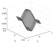
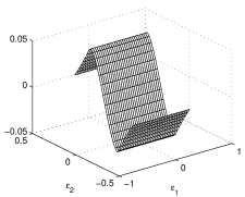
Figure 3: Map of the discretization error $x_{g}-\varepsilon_{1}$ (left) and $y_{g}-\varepsilon_{2}$ (right) for an array of parallelogram detectors with $\tau_{1}=\tau_{2}=1$ and $\alpha=2$. The signal distribution is a disk with radius $R=1.5\tau$.

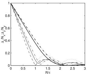
Figure 4: Average square errors of the array in Fig. 3 for a set of signal distributions with radius $R$, normalized to the square errors of a Dirac $\delta$-distribution. The dashed line is the $\Delta_{x_{g}}$ for rectangles, the dotted lines is $\Delta_{y_{g}}$. The solid line is $\Delta_{x_{g}}$ for disks, the dashed-dotted line is $\Delta_{y_{g}}$. The thick lines are the errors for conic-like form given by the convolution of two disks.

$y_{g}/\alpha$ and $\varepsilon_{2}/\alpha$ dependence, thus, when $\alpha\rightarrow\infty$, the two COG errors decouple and $x_{g}$ has no dependence on $\varepsilon_{2}$. Hence, it becomes identical to that calculated in [1]. In all the other cases, mixed dependence on $\varepsilon_{1}$ and $\varepsilon_{2}$ is to be expected. Applying Eq. (19) with g${}^{p}(\boldsymbol{\varepsilon})$ in place of g$(\boldsymbol{\varepsilon})$, we find the average square errors:

$$\Delta_{x}^{2}= \big{(}\frac{\tau_{1}^{2}}{2\pi^{2}}\big{)}\ \sum_{m=1}^{+\infty}\frac{1}{m^{2}}\big{|}\Phi(-m\mathbf{r}_{1})\big{|}^{2}+\frac{\Delta_{y}^{2}}{\alpha^{2}}$$ (22)

$$\Delta_{y}^{2}= \big{(}\frac{\tau_{2}^{2}}{2\pi^{2}}\big{)}\ \sum_{k=1}^{+\infty}\frac{1}{k^{2}}\big{|}\Phi(-k\mathbf{r}_{2})\big{|}^{2}.$$ (23)

Figure 3 illustrates the two-dimensional map of the discretization errors of $x_{g}$ and $y_{g}$ of Eqs. (20,21) for a disk-shape signal distribution of radius $R=1.5\,\tau$. Here we can appreciate the differences of $x_{g}$ and $y_{g}$: $(x_{g}-\varepsilon_{1})$ shows a simultaneous dependence on $\varepsilon_{1}$ and $\varepsilon_{2}$, and $(y_{g}-\varepsilon_{2})$ does not depend on $\varepsilon_{1}$. This is typical of all the parallelogram detectors.

Figure 4 plots the average errors in Eqs. (22,23) with $R$ increasing from zero to $3\tau$ for various forms of signal distributions. The errors are normalized to the value of the error for a Dirac $\delta$-function signal distribution ($N_{x}^{2}=\tau_{1}^{2}/12+N_{y}^{2}/\alpha$ and $N_{y}^{2}=\tau_{2}^{2}/12$).

The thin dashed and dotted lines refer to a square signal distribution: The zeros are given by the $sinus$ functions present in the FT. The thin solid and dashed-dotted lines are the errors (on $x_{g}$ and $y_{g}$) of a disk. The origin of the diffraction-like aspect of the average errors is given by the zeros of the J${}_{1}(\omega)$ (Bessel function of the first kind) which eliminates the $m=1$ or $k=1$ terms of (22) and (23), leaving only smaller higher order terms.

The thick solid and dashed-dotted lines are the errors of a conic-like signal distribution given by the convolution of two identical disks. Its FT is the square of the FT of a disk. We can see that, above $R/\tau=2$, the COG discretization error practically disappears. This is due to the first double zeros of J${}_{1}(\omega)^{2}$ whose effects tends to overlap, thereby almost completely suppressing the COG discretization error for this signal distribution. This approximate cancellation is interesting for its efficiency.

4.2 Hexagons

As stated above, the sampling along the lines of a set of parallelograms is able to handle other types of detectors as well.

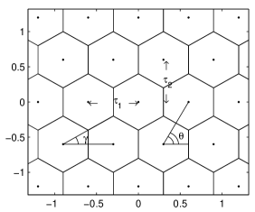
Figure 5: Array of hexagonal detectors, $\tau_{1}$ and $\tau_{2}$ are the x-distance and y-distance of the centers of two neighboring detectors. The angle $\theta$ is the bending of the parallelogram as in Fig. 2, here $\tan(\theta)=2\tau_{2}/\tau_{1}$. The angle $\gamma$ is the inclination of the upper and lower sides of the hexagons.

Figure 5 illustrates a hexagonal array showing the parallelogram sampling strategy. An example of a detector with a mosaic of hexagons is the 61-pixels HPD of DEP [7]. We shall limit ourselves to hexagons with two sides parallel to the $y$-axis. Other types such as those with two sides inclined with respect to the $y$-axis would be allowed, but, since we do not know of any detector of this type, we shall ignore them.

As is evident in Fig. 5, $\alpha=\tan(\theta)=\frac{2\tau_{2}}{\tau_{1}}$, and only $\tau_{1}$ and $\tau_{2}$ are the free parameters defining the array; any other parameter can be reduced to them. The angle $\gamma$ is formed by the inclined lata with respect to the $x$-axis. It turns out that $\beta=\tan(\gamma)=\frac{2\tau_{2}}{3\tau_{1}}$, and now $\mathbf{n}_{1}=(\tau_{1}\,;\,0)$ and $\mathbf{n}_{2}=(\tau_{1}/2\,;\,\tau_{2})$. Regular hexagons are obtained with $\gamma=\frac{\pi}{6}$ so $\frac{\tau_{2}}{\tau_{1}}=\frac{\sqrt{3}}{2}$. To apply the equations in Section 2, we need the FT of a hexagon, which can be calculated by:

$$\mathrm{G}^{h}(\omega_{x};\omega_{y})=\int_{-\frac{\tau_{1}}{2}}^{+\frac{\tau_{1}}{2}}\mathrm{d}x\int_{\mathrm{y}_{1}(x)}^{\mathrm{y}_{2}(x)}\mathrm{d}y\,\mathrm{e}^{-i(\omega_{x}x+\omega_{y}y)}$$

where y${}_{1}(x)$ and y${}_{2}(x)$ are the two set of lines:

$$\mathrm{y}_{1}(x) =-\beta x-\frac{2}{3}\tau_{2}\ \ \ \ \mathrm{y}_{1}(x)=\beta x-\frac{2}{3}\tau_{2}$$

$$\ \ \ \ \ x<0\ \ \ \ \ \ \ \ \ x\geq 0$$

$$\mathrm{y}_{2}(x) =\ \beta x+\frac{2}{3}\tau_{2}\ \ \ \quad \mathrm{y}_{2}(x)=-\beta x+\frac{2}{3}\tau_{2}.$$

With some effort, G${}^{h}(\omega_{x};\omega_{y})$ assumes the form (one among the many possible):

$$\mathrm{G}^{h}(\omega_{x};\omega_{y})=\frac{\tau_{1}}{\omega_{y}}\big{[} \sin(\frac{\omega_{x}\tau_{1}}{4}+\frac{\omega_{y}\tau_{2}}{2})\mathrm{sinc}(\frac{\omega_{x}\tau_{1}}{4}-\frac{\omega_{y}\tau_{2}}{6})-$$

$$\sin(\frac{\omega_{x}\tau_{1}}{4}-\frac{\omega_{y}\tau_{2}}{2})\mathrm{sinc}(\frac{\omega_{x}\tau_{1}}{4}+\frac{\omega_{y}\tau_{2}}{6})\big{]}\ .$$

This form allows easy verification of Eq. (17):

$${\underset{\begin{subarray}{c}\boldsymbol{\omega}\rightarrow 0\end{subarray}}{\mathrm{lim}}}\mathrm{G}^{h}(\boldsymbol{\omega}-m\mathbf{r}_{1}-k\mathbf{r}_{2})=\tau_{1}\tau_{2}\delta_{m,0}\ \delta_{k,0}\ .$$

Now, $\mathbf{r}_{1}=(2\pi/\tau_{1}\,;\,-\pi/\tau_{2})$ and $\mathbf{r}_{2}=(0\,;\,2\pi/\tau_{2})$ are reintroduced, and, as expected, this hexagon array saves the normalization of $\varphi(\mathbf{x})$.

The calculation of G${}_{x}^{h}$ and G${}_{y}^{h}$ is a bit more complicated, and some help is required of mathematica [8]. An easy form which coincides with the partial derivative at $m,k\in\mathbb{Z}^{2}$ (as is our concern) can be derived:

$${\underset{\begin{subarray}{c}\boldsymbol{\omega}\rightarrow 0\end{subarray}}{\mathrm{lim}}}\mathrm{G}_{x}^{h}(\boldsymbol{\omega}-m\mathbf{r}_{1}-k\mathbf{r}_{2}) =\frac{9m\tau_{1}^{2}\tau_{2}\sin\big{(}2(m+k)\frac{\pi}{3}\big{)}}{4(m-2k)(2m-k)(m+k)\pi^{2}}\ \ \ m\neq 2k\ \ 2m\neq k\ \ m\neq-k$$

$$=-\frac{\tau_{1}^{2}\tau_{2}}{6k\pi}\ \ \ \quad m=2k$$

$$=-\frac{\tau_{1}^{2}\tau_{2}}{12m\pi}\ \ \ \ k=2m\ \ \ k=-m\ .$$

Using a similar procedure, we can obtain a simplified form of the partial derivative of G${}^{h}(\boldsymbol{\omega})$ with respect to $\omega_{y}$ for $m,k\in\mathbb{Z}^{2}$:

$${\underset{\begin{subarray}{c}\boldsymbol{\omega}\rightarrow 0\end{subarray}}{\mathrm{lim}}}\mathrm{G}_{y}^{h}(\boldsymbol{\omega}-m\mathbf{r}_{1}-k\mathbf{r}_{2}) =\frac{-3\tau_{1}\tau_{2}^{2}\sin\big{(}2(m+k)\frac{\pi}{3}\big{)}}{2(2m-k)(m+k)\pi^{2}}\ \ \ 2m\neq k\ \ m\neq-k$$

$$=-\frac{\tau_{1}\tau_{2}^{2}}{6m\pi}\ \ \ \quad k=2m$$

$$=\ \ \frac{\tau_{1}\tau_{2}^{2}}{6m\pi}\ \ \ \quad k=-m$$

For $k=0$ and $m=0$, G${}_{x}^{h}(0)$ and G${}_{y}^{h}(0)$ are the hexagon COG-coordinates, and these are zero for our choice of the reference system origin.

Selecting a signal distribution, we can use Eq. (18) to calculate the COG discretization error for the hexagonal detector array. The center $(\boldsymbol{\varepsilon})$ of the signal distribution must cover a hexagon, and, due to the periodicity of the array, the error identically reproduces for all the other hexagons.

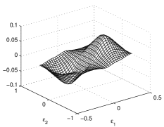
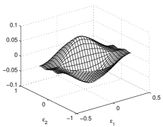
Figure 6: Map of the discretization error $x_{g}-\varepsilon_{1}$ (left) and $y_{g}-\varepsilon_{2}$ (right) for an array of hexagonal detectors with $\tau_{1}=\tau_{2}=1$. The signal distribution is a disk with radius $R=1.5\tau$.

The two errors are shown in Fig. 6. They are evidently different with respect to the parallelogram array in Fig. 3. Now, the $(x_{g}-\varepsilon_{1})$ and $(y_{g}-\varepsilon_{2})$ simultaneously depend on $\varepsilon_{1}$ and $\varepsilon_{2}$. The effect of the hexagon’s symmetric points eliminates the discretization error on the vertices and in the middle. Being less symmetric, the parallelograms have a larger discretization error.

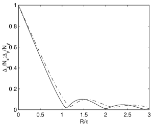
Figure 7: Average square errors of an array of hexagonal detectors ($\tau_{1}=\tau_{2}=1$) for a disk signal distributions with radius $R$ normalized to the square error of a Dirac $\delta$-distribution on a hexagon.

The average square errors can be calculated with Eq. (19). Figure 7 illustrates the results of its application which in this case is normalized to the errors of a Dirac $\delta$-function on a hexagon (N${}_{x}^{2}=5\tau_{1}^{2}/72$ and N${}_{y}^{2}=5\tau_{2}^{2}/54$). The plots in Fig. 7 greatly resemble those in Fig. 4. This is due to the normalization which always initializes the plots to one. The normalization constants are smaller for the hexagon compared to the parallelogram. As in Fig. 4, the minima are given by the zeros of the J${}_{1}(\omega)$, the FT of a disk. The noticeable effect of the zeros assures that the higher-order terms of the double infinite series of Eq. (19) contribute only modestly to the results. As the other types of signal distributions in Fig. 4 resemble them, they are not illustrated.

4.3 Triangles

Detectors with triangular sections are rarely used in high energy physics, an exception is the Crystal Ball [2]. The Crystal Ball calorimeter is composed of $672$ $NaI$ crystals in the form of a truncated pyramid with a triangular base. Each crystal points to the center of the sphere which circumscribes the calorimeter. The crystal dimensions and the two-dimensional arrangement are chosen so that the crystals fit inside two sealed hemispherical containers.

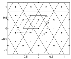
Figure 8: Array of triangular detectors: $\tau_{1}$ is the $x$-distance of the COG of two neighboring detectors, $\tau_{2}$ is the $y$-distance, $\theta$ is the bending angle of the inclined sides. Triangles with a point in the COG are sampled together with the sampling cell indicated by the solid-line parallelogram. Triangles with asterisk in the COG are sampled together and the dashed-dotted parallelogram is their sampling cell.

The spherical geometry can be approximated by our planar distribution only on a small region.

The sampling differs greatly from the cases considered so far. First, we have to observe (Fig. 8) that two different types of triangles are involved: One with a vertex pointing toward the $x$-axis (indicated in Fig. 8 by a dot in the COG) and one oriented in the opposite direction (indicated in Fig. 8 by an asterisk in the COG). Therefore, two samplings are required. The periodicity of the samplings is identical, and a parallelogram is the elementary cell. The sampling cell is shifted a fixed amount with respect to the other, and two different convolutions f${}_{\boldsymbol{\varepsilon}}(\mathbf{x})$ are sampled. Let us call f${}_{1}(\mathbf{x})$ the first convolution with the triangle pointing downward and f${}_{2}(\mathbf{x})$ the convolution with the triangle pointing upward:

$$\mathrm{f}_{1}(\mathbf{x})=\int_{\mathbb{R}^{2}}\mathrm{d}\mathbf{x}^{\prime}\,\mathrm{g}_{1}(\mathbf{x}-\mathbf{x}^{\prime})\,\varphi(\mathbf{x}^{\prime})\,,$$ (24)

$$\mathrm{f}_{2}(\mathbf{x})=\int_{\mathbb{R}^{2}}\mathrm{d}\mathbf{x}^{\prime}\,\mathrm{g}_{2}(\mathbf{x}-\mathbf{x}^{\prime})\,\varphi(\mathbf{x}^{\prime})\,.$$

We will only consider isosceles triangles. From Fig. 8, we can see that $\alpha=\tan\theta=2\tau_{2}/\tau_{1}$.

Let us define the samplings. The first is generated by a set of products of Dirac $\delta$-functions centered on the points $\{n\tau_{1}+l\tau_{1}/2;l\tau_{2}\},n,l\in\mathbb{Z}^{2}$. The second is generated by a set of products of Dirac $\delta$-functions centered on the points shifted by $\Delta_{2}$ in the $y$-direction $\{n\tau_{1}+l\tau_{2}/\alpha;l\tau_{2}+\Delta_{2}\},n,l\in\mathbb{Z}^{2}$ where $\Delta_{2}=\frac{2}{3}\tau_{2}$ (and $\boldsymbol{\Delta}_{2}=(0\,;\,\Delta_{2})$) is the shift of the COG of the second type of triangle from that of the first type centered in the origin (Fig. 8). With these positions, s${}_{\boldsymbol{\varepsilon}}(\mathbf{x})$ becomes:

$$\begin{split}\mathrm{s}_{\boldsymbol{\varepsilon}}(\mathbf{x})=\sum_{n,l}\ &\big{[}\ \delta(\mathbf{x}-n\mathbf{n}_{1}-l\mathbf{n}_{2})\,\mathrm{f}_{1}(n\mathbf{n}_{1}+l\mathbf{n}_{2}-\boldsymbol{\varepsilon})+\\ &\delta(\mathbf{x}-n\mathbf{n}_{1}-l\mathbf{n}_{2}-\boldsymbol{\Delta}_{2})\mathrm{f}_{2}(n\mathbf{n}_{1}+l\mathbf{n}_{2}+\boldsymbol{\Delta}_{2}-\boldsymbol{\varepsilon})\big{]}.\end{split}$$ (25)

The first term accounts for the first set of samplings; the second term is the shifted sampling on the second type of triangles.

Up to now, we have paid no attention to the difference in the definition of the detector forms and the function g$(\mathbf{x})$. We considered them identical, a simplification allowed by the symmetry of the forms used (rectangles, parallelograms, and hexagons). Since the triangles are not symmetric with respect to their COGs, i.e., g${}_{1,2}(x,y)\neq$g${}_{1,2}(-x,-y)$, we only have a symmetry with respect to the $y$-axis, i.e., g${}_{1,2}(x,y)=$g${}_{1,2}(-x,y)$). This difference must be highlighted and isolated to avoid incorrect results. The double sampling implies phase differences which must be recovered by the phase differences of the FTs of the triangles which are no longer real. The detector form can be indicated by the function:

$$z=\mathrm{g}_{d}(x-x_{0},y-y_{0})$$ (26)

where $z$ is the surface generated by g_d for the downward triangle (g_u for the upward). It has a constant value or it is zero and is centered in $x_{0}$ and $y_{0}$ where $x_{0}$, $y_{0}$ are the coordinates of the detector COG. Comparing Eq. (26) with Eqs. (24) and (25), we find the differences: Eq. (24) contains g${}_{1}(x_{0}-x^{\prime};y_{0}-y^{\prime})$ where $x_{0}$ and $y_{0}$ are now the coordinates of the detector COG, yielding:

$$\mathrm{g}_{1}(x_{0}-x;y_{0}-y)=\mathrm{g}_{d}(-(x-x_{0});-(y-y_{0})).$$ (27)

For symmetric detectors, this difference is irrelevant, but for triangles it represents a complete inversion. In fact, having defined g${}_{d}(\mathbf{x})$ as the first type of triangle, we find g${}_{d}(-\mathbf{x})$ as the second type. If we incorrectly take for g${}_{1}(\mathbf{x})$ the function g${}_{d}(\mathbf{x})$ in the convolution (24), the function g${}_{1}(-\mathbf{x})$ is actually used. This implies an exchange between the two types of triangles; Eq. (17) is no longer verified due to the overlap of the triangles and the holes left in the plane. Let us calculate the form of G${}_{d}(\boldsymbol{\omega})$ the FT of g${}_{d}(\mathbf{x})$, and S${}_{\boldsymbol{\varepsilon}}(\boldsymbol{\omega})$ the FT of s${}_{\boldsymbol{\varepsilon}}(\mathbf{x})$. The function g${}_{d}(x,y)$ can be expressed by the interval function $\Pi(x)$ as defined in Section 3.1:

$$\mathrm{g}_{d}(x,y)=\Pi(\frac{y+\frac{\tau_{2}}{6}}{\tau_{2}})\Pi(\frac{x}{\frac{2}{\alpha}(y+\frac{2}{3}\tau_{2})})$$ (28)

$$\mathrm{G}_{d}(\omega_{x};\omega_{y})=\int_{-\frac{2}{3}\tau_{2}}^{\frac{1}{3}\tau_{2}}\mathrm{d}y\int_{-(y+\frac{2}{3}\tau_{2})\frac{1}{\alpha}}^{(y+\frac{2}{3}\tau_{2})\frac{1}{\alpha}}\mathrm{d}x\mathrm{e}^{-i(\omega_{x}x+\omega_{y}y)}\ .$$

Among the forms of G${}_{d}(\omega_{x};\omega_{y})$ we shall indicate:

$$\begin{split}\mathrm{G}_{d}(\omega_{x};\omega_{y})=\frac{4\tau_{1}\tau_{2}\ \mathrm{e}^{-i\frac{\omega_{y}\tau_{2}}{3}}}{(4\omega_{y}^{2}\tau_{2}^{2}-\omega_{x}^{2}\tau_{1}^{2})}\big{[}\cos(\frac{\omega_{x}\tau_{1}}{2})-\mathrm{e}^{i\omega_{y}\tau_{2}}+i\omega_{y}\tau_{2}\ \mathrm{sinc}(\frac{\omega_{x}\tau_{1}}{2})\big{]}\,.\end{split}$$ (29)

Due to the double sampling, the calculation of the FT of s${}_{\boldsymbol{\varepsilon}}(\mathbf{x})$ becomes more complicated. With two applications of the procedure described for Eq. (14), the Poisson relation for this case can be derived as:

$$\mathrm{S}_{\boldsymbol{\varepsilon}}(\boldsymbol{\omega})= \sum_{m,k}\mathrm{e}^{-i(\boldsymbol{\omega}-\mathbf{L}_{m\,k})\cdot\boldsymbol{\varepsilon}}\big{[}\mathrm{G}_{d}^{*}(\boldsymbol{\omega}-\mathbf{L}_{m\,k})+\mathrm{e}^{i(m-2k)\frac{2}{3}\pi}\mathrm{G}_{d}(\boldsymbol{\omega}-\mathbf{L}_{m\,k})\big{]}\Phi(\boldsymbol{\omega}-\mathbf{L}_{m\,k})$$

$$\mathbf{L}_{m\,k}= m\mathbf{r}_{1}+k\mathbf{r}_{2}=\big{(}\frac{2m\pi}{\tau_{1}}\,;\,\frac{\pi}{\tau_{2}}(2k-m)\big{)}$$

where G${}_{d}^{*}(\boldsymbol{\omega})$ is the complex conjugate of G${}_{d}(\boldsymbol{\omega})$ defined by Eq. (28) and is the FT of g${}_{2}(x,y)$ of Eq. (24) as explained above.

We can verify that G${}_{d}(-\mathbf{L}_{m\,k})$ becomes zero for integers $m\neq 0$ and $k\neq 0$; nonzero contributions are obtained when $m=0$ and $k\neq 0$ or $m\neq 0$ and $k=0$. These terms are cancelled out by G${}^{*}_{d}$. The phase factor behind G_d in Eq. (LABEL:eq:FTstria) is crucial for the cancellation: Only the term with $m=0$ and $k=0$ survives, and Eq. (17) is verified. The sampling arrangement of Eq. (25) effectively tessellates the plane with triangular detectors.

The combination of two triangles, one pointing upward and the other downward, forms a parallelogram. This property simplifies the partial derivatives of S${}_{\boldsymbol{\varepsilon}}(\boldsymbol{\omega})$, and the nonzero elements needed to calculate the COG are:

$$\mathrm{G}^{t}(\boldsymbol{\omega})=\mathrm{G}_{d}^{*}(\boldsymbol{\omega})+\mathrm{e}^{i\pi\frac{2}{3}(m-2k)}\mathrm{G}_{d}(\boldsymbol{\omega})$$ (31)

$${\underset{\begin{subarray}{c}\boldsymbol{\omega}\rightarrow 0\\ k=0\end{subarray}}{\mathrm{lim}}}\mathrm{G}_{x}^{t}(\boldsymbol{\omega}-\mathbf{L}_{m\,0})=$$

$${\underset{\begin{subarray}{c}\boldsymbol{\omega}\rightarrow 0\\ k=m\end{subarray}}{\mathrm{lim}}}\mathrm{G}_{x}^{t}(\boldsymbol{\omega}-\mathbf{L}_{m\,m})=\frac{-\tau_{1}^{2}\tau_{2}}{4}\frac{\mathrm{e}^{-i\frac{4}{3}m\pi}}{m\pi}$$

for $m$ integer and $m\neq 0$. Similarly, G${}_{y}^{t}$ is:

$${\underset{\begin{subarray}{c}\boldsymbol{\omega}\rightarrow 0\\ k=0\end{subarray}}{\mathrm{lim}}}\mathrm{G}_{y}^{t}(\boldsymbol{\omega}-\mathbf{L}_{m\,0})=$$ (32)

$${\underset{\begin{subarray}{c}\boldsymbol{\omega}\rightarrow 0\\ k=m\end{subarray}}{\mathrm{lim}}}\mathrm{G}_{y}^{t}(\boldsymbol{\omega}-\mathbf{L}_{m\,m})=\frac{\tau_{1}\tau_{2}^{2}}{6}\frac{\mathrm{e}^{-i\frac{2}{3}m\pi}}{m\pi}$$

for $m\neq 0$ and $m$ integer. Using Eqs. (31) and (32), we can calculate $x_{g}$ and $y_{g}$, which turn out to be:

$$x_{g}= \varepsilon_{1}+\frac{\tau_{1}}{2\pi}\sum_{m=1}^{+\infty}\frac{1}{m}\mathrm{Imag}\Big{\{}\mathrm{e}^{im\pi(\frac{2\varepsilon_{1}}{\tau_{1}}-\frac{4}{3})}\big{[}\mathrm{e}^{-i\frac{m\pi}{\tau_{2}}\varepsilon_{2}}\Phi(-\mathbf{L}_{m\,0})+\mathrm{e}^{i\frac{m\pi}{\tau_{2}}\varepsilon_{2}}\Phi(-\mathbf{L}_{m\,m})\big{]}\Big{\}}$$

$$y_{g}= \varepsilon_{2}-\frac{\tau_{2}}{3\pi}\sum_{m=1}^{+\infty}\frac{1}{m}\mathrm{Imag}\Big{\{}\mathrm{e}^{im\pi(\frac{2\varepsilon_{1}}{\tau_{1}}-\frac{2}{3})}\big{[}\mathrm{e}^{-i\frac{m\pi}{\tau_{2}}\varepsilon_{2}}\Phi(-\mathbf{L}_{m\,0})+\mathrm{e}^{i\frac{m\pi}{\tau_{2}}\varepsilon_{2}}\Phi(-\mathbf{L}_{m\,m})\big{]}\Big{\}}.$$

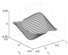
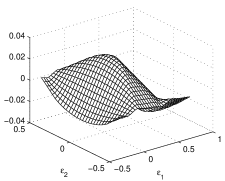
Figure 9: Map of the discretization error $x_{g}-\varepsilon_{1}$ (left) and $y_{g}-\varepsilon_{2}$ (right) for an array of triangular detectors as in Fig. 8, but calculated on a rectangular-elementary cell. The signal distribution is again a disk with radius $R=1.5\tau$.

Although the two sums in Eq. (LABEL:eq:COGtria) look identical, they actually differ by a phase factor contained in the first exponential. For Eq. (19), this phase difference is irrelevant for the square mean errors $\Delta_{x}^{2}$ and $\Delta_{y}^{2}$ that become proportional, and are given by:

$$\Delta_{x}^{2}=\tau_{1}^{2}\sum_{m=1}^{+\infty}\frac{1}{8m^{2}\pi^{2}}\Big{[}\big{|}\Phi(-\mathbf{L}_{m\,0})\big{|}^{2}+\big{|}\Phi(-\mathbf{L}_{m\,m})\big{|}^{2}\Big{]}$$ (34)

$$\Delta_{y}^{2}=\frac{4\tau_{2}^{2}}{9\tau_{1}^{2}}\Delta_{x}^{2}\ .$$

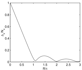
Figure 10: Average square errors of an array of triangular detectors ($\tau_{1}=\tau_{2}=1$) for a disk signal distribution with radius $R$ ranging from zero to $3\tau_{1}$ normalized to the square error of a Dirac $\delta$-distribution.

In the plots of $(x_{g}-\varepsilon_{1})$ and of $(y_{g}-\varepsilon_{2})$ shown in Fig. 9, the elementary cell is taken as a rectangle because, in the case of axisymmetric signal distribution, a few lines parallel to the $y$-axis have zero discretization error. Figure 10 shows $\Delta_{x,y}$. From the second equation (34), we can see that the normalized errors $\Delta_{x,y}$ are now identical, the errors are always proportional, and the normalization reabsorbs the constant. Here, too, the average square error is suppressed for the disk signal distribution of special sizes, which is always produced by the zeros of the J${}_{1}(\omega)$ Bessel function (FT of a disk).

5 Special Signal Distributions

5.1 Signal Distributions Free of Discretization Error

In the previous sections, we illustrated the properties of some detector arrays. Our selection only partially covers the richness of possible configurations allowed by the two-dimensional geometry as compared with the one-dimensional geometry. We encounter a similar large set of configurations for signal distributions free of discretization error.

The easiest case of band-limited functions has some additional properties. From Eq. (19), we can see that $\Phi(\boldsymbol{\omega})$ has two different band-limits: $\Phi(\omega_{x},\omega_{y})=0$ for $|\omega_{x}|\geq 2\pi/\tau_{1}$ and $|\omega_{y}|\geq 2\pi/\tau_{2}$. If the FT of $\varphi(\mathbf{x})$ has these limitations, $\Delta_{x}^{2}$ and $\Delta_{y}^{2}$ are always zero, no matter what type of detectors are considered, granted that the detector array has a periodicity controlled by parameters $\tau_{1}$ and $\tau_{2}$. Roughly speaking, we can say that, even in two dimensions, the origin of the discretization error $\Delta_{x,y}$ can be connected to the aliasing effects due to the improper sampling of the function f${}_{\boldsymbol{\varepsilon}}(\mathbf{x})$ with overly large sampling steps for the band-limits (if any) of the function $\varphi(\mathbf{x})$. The band boundaries which could eliminate the discretization error are twice those required by the Wittaker-Kotel’nikov-Shannon (WKS) sampling theorem [10, 6] for a complete reconstruction of the function f${}_{\boldsymbol{\varepsilon}}(\mathbf{x})$ from their sampled values at intervals $\tau_{1}$ and $\tau_{2}$.

As demonstrated in Ref. [6, 11], a band-limited function cannot be zero on any finite part of the plane. This property rules out these functions from the set of functions usually encountered in experimental position measurements. Here, the functions $\varphi(\mathbf{x})$ become zero after only a few $\tau_{1}$ or $\tau_{2}$, and no band-limitations can be invoked or postulated. The elimination of the COG discretization error can be obtained from other sources. We can see in some of the previous figures that the discretization error disappears for special forms and special sizes.

In the one-dimensional case, the interval function and all its convolutions with normalized functions have sizes without discretization error. In two dimensions, this set is much larger. It is evident from Eq. (19) that: All the signal distributions with the property of Eq. (17) with the same $\{\alpha,\tau_{1},\tau_{2}\}$ as the detector array are free of COG-discretization error. For example, for $\alpha=2$ we explicitly demonstrate that a hexagonal distribution has the property (17). Therefore, a hexagonal signal distribution with sizes $\tau_{1}$ and $\tau_{2}$ or any of their multiples (and all the other related parameters as described in Fig. 5) has an exact $x,y$-COG on an array of isosceles triangles with base $\tau_{1}$ and height $\tau_{2}$ and arranged as in Fig. 8. Highly irregular shapes such as those illustrated in Ref. [4] are prototypes of signal distributions free of the COG discretization errors. We can easily prove from the previous equations that even disconnected signal distributions have an exact COG. For example, any two triangles (one pointing upward and one downward) in Fig. 8 have exact COGs on the hexagon array in Fig. 5. Each triangle has a COG error, but, paired, the errors cancel out.

Evidently, all the convolutions of arbitrary functions with functions having the property (17) continue to maintain it and are free of COG-discretization errors. A rectangular signal distribution of dimensions $\tau_{1}$ and $\tau_{2}$ (or any of their multiples) is free of discretization error for any array with the same $\tau_{1}$, $\tau_{2}$ and any value of $\alpha$. We can easily figure out the geometric origin of the property. An array of rectangles of dimensions $\{\tau_{1},\tau_{2}\}$, where each line of detectors is shifted with respect to the previous line of a fixed amount $\sigma$ tessellate the plane. Therefore, Eq. (17) must hold, and due to $\alpha=\tau_{2}/\sigma$ any type of array with the values $\{\tau_{1},\tau_{2},\alpha\}$ is easily generated. Even the parallelogram and triangle arrays continue to tessellate the plane after a shift of one detector line with respect to another and when the shift is repeated in all the detector lines. In the following subsection, we will describe a few properties of arrays of shifted rectangles.

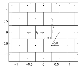
Figure 11: Array of shifted rectangular detectors. $\tau_{1}$ and $\tau_{2}$ are defined as usual. $\sigma$ is the shift of the detector centers of a row with respect to the detector centers of the row below them. Tan$(\theta)=\tau_{2}/\sigma$ is the bending angle of the line connecting the centers of two rectangles pertaining to two different rows.

5.2 Shifted Rectangles

To exemplify the property of an array of shifted detectors, we shall describe the easiest one, i.e., that of the array of shifted rectangles (Fig. 11). It is evident that, at the variation of the shift $\sigma$, all the values of $\alpha=\tan(\theta)=\tau_{2}/\sigma$ are explored, and Eq. (10)-(19) must be applied to the sampling. The FT of g${}^{r}(x,y)$ of a rectangle is given by:

$$\mathrm{G}^{r}(\omega_{x},\omega_{y})=\tau_{1}\tau_{2}\,\mathrm{sinc}(\frac{\omega_{x}\tau_{1}}{2})\,\mathrm{sinc}\big{(}\frac{\omega_{y}\tau_{2}}{2}\big{)}.$$

Writing Eq. (17) for this case, we get:

$$\mathrm{G}^{r}(-m\mathbf{r}_{1}-k\mathbf{r}_{2})=\tau_{1}\tau_{2}\,\mathrm{sinc}(-m\pi)\,\mathrm{sinc}\big{(}\frac{2m\pi\tau_{2}}{\tau_{1}\alpha}-k\pi\big{)}=\tau_{1}\tau_{2}\,\delta_{m,0}\,\delta_{k,0}\ .$$ (35)

where the first $sinc$-function eliminates any $m$ and $\alpha$ dependence in the second one. The tessellation condition is verified for any $\alpha$ as expected by naive intuition. Equation (35) is what we need to prove that a rectangular form of dimensions $\tau_{1}$ and $\tau_{2}$ (and all the multiples of these dimensions) is free of discretization error for any array with the same $\tau_{1}$ and $\tau_{2}$, any $\alpha$ and any form of detectors which tessellate the plane. We can easily verify that the same is true for parallelograms and triangles. The hexagons cannot be shifted.

5.3 Scaled Signal Distributions

In discussing Eq. (17), we considered an array of detectors covering the plane, but among the periodic forms that satisfy Eq. (17), we have to consider their scaled forms. For the scaling property of the FT, if we define $\mathrm{g}_{l}(\mathbf{x})=\mathrm{g}(\mathbf{x}/l)/l^{2}$ than $\mathrm{G}_{l}(\boldsymbol{\omega})=\mathrm{G}(l\boldsymbol{\omega})$. Thus, if $\mathrm{g}(\mathbf{x})$ satisfies Eq. (17), then $\mathrm{g}_{l}(\mathbf{x})$ satisfies the same equation for any positive integer $l$. The normalized signal distribution $\varphi(\mathbf{x})=\mathrm{g}_{l}(\mathbf{x})/(\tau_{1}\tau_{2})$ is free of discretization error. As detectors, the functions $\mathrm{g}_{l}(\mathbf{x})$ have crosstalk with the neighboring detectors.

5.4 Approximate Results

Some previous figures of the average square errors report deep minima for some R-values of disk-shaped signal distribution. These minima do not reach zero values of the square error, but are always suppressions of the COG discretization error worthy of exploration. For this reason, all the plots in Eq. (19) exhibit the error for the disk signal distribution. Cell bending $\alpha$ has some effect on the minima positions. For parallelograms and hexagons, we can see a slight shift in the minimum for $\Delta_{x}$ and $\Delta_{y}$ and $\alpha=2$, for larger $\alpha$-values the shift tends to disappear as can be verified from Eqs. (22) and (23) for parallelograms. The FT of a disk is $4J_{1}(R\omega)/(R\omega)$, and the discretized values of $\omega_{x}$ and $\omega_{y}$ modulate the effect of the zeros of $J_{1}(\omega)$ in Eq. (19), giving a shift of the minimum. The interesting aspect of this approximate result is its applicability to almost all the detector arrays as far as $\tau_{1}\sim\tau_{2}$.

6 Crosstalk and Loss

6.1 Loss

If the detectors in the array have generic (nonuniform) crosstalk or they have some losses, Eq. (16) need some modification. We must consider:

$$\mathrm{S}_{\boldsymbol{\varepsilon}}(0)=\sum_{nl}\mathrm{f}(n\mathbf{n}_{1}+l\mathbf{n}_{2}-\boldsymbol{\varepsilon})\leq 1\ .$$ (36)

The detector array does not generate a constant (over the plane) efficiency function, and in some regions the efficiency drops below one. Now S${}_{\boldsymbol{\varepsilon}}(0)$ retains its dependence on the position and form of the signal distribution, and Eq. (17) is no longer valid. To calculate the COG, we have to use Eq. (12) with the partial derivatives of $\Phi(\boldsymbol{\omega})$:

$$\mathbf{r}_{g}=\boldsymbol{\varepsilon}+\frac{i}{\tau_{1}\tau_{2}\mathrm{S}_{\boldsymbol{\varepsilon}}(0)}\,\sum_{m,\,k}\mathrm{e}^{i\mathbf{L}_{m\,k}\cdot\,\boldsymbol{\varepsilon}}[\,\mathrm{\mathbf{G}}_{\boldsymbol{\omega}}(-\mathbf{L}_{m\,k})\Phi(-\mathbf{L}_{m\,k})+\mathrm{G}(-\mathbf{L}_{m\,k})\boldsymbol{\Phi}_{\boldsymbol{\omega}}(-\mathbf{L}_{m\,k})\big{]}$$ (37)

$$\mathbf{L}_{m\,k}=m\mathbf{r}_{1}+k\mathbf{r}_{2}=\big{(}\frac{2m\pi}{\tau_{1}}\,;\,-\frac{2m\pi}{\tau_{1}\alpha}+\frac{2k\pi}{\tau_{2}}\big{)}\,.$$

Here, $\boldsymbol{\Phi}_{\boldsymbol{\omega}}=(\Phi_{x}\,;\,\Phi_{y})$ is the vector of the partial derivatives with respect to $\omega_{x}$ and $\omega_{y}$ of $\Phi(\omega_{x},\omega_{y})$. Equation (37) allows some simplification if the signal distribution is one of the special

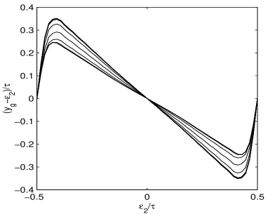
Figure 12: Set of error curves ($\varepsilon_{2}-\tau_{2}$) for a signal distribution formed by two disks, one of small radius (0.15 $\tau$) and considerable height (4.5), and a disk with a larger radius (1.5 $\tau$) and relative height 1; the detectors are squares with a region of loss at any border for a range of $0.025\tau$.

functions discussed in Section 4. If $\varphi(\mathbf{x})$ is a band-limited function with $\Phi(\omega_{x},\omega_{y})=0$ for $|\omega_{x}|\geq 2\pi/\tau_{1}$ and $|\omega_{y}\geq 2\pi/\tau_{2}$, the COG discretization error disappears for any type of loss or crosstalk; in this case, S${}_{\boldsymbol{\varepsilon}}(0)$ is always constant. If $\varphi(\mathbf{x})$ is one of the finite support functions which have no COG error in absence of loss (or crosstalk), S${}_{\boldsymbol{\varepsilon}}(0)$ is constant for any g$(\mathbf{x})$, and only the terms depending on the partial derivatives of $\Phi(\boldsymbol{\omega})$ remain in Eq. (37). For functions whose first partial derivatives pertain to previous class, even the last term of Eq. (37) disappears for any type of loss or crosstalk.

Figure 12 shows one of the loss effects, i.e., the introduction of a simultaneous dependence on $\varepsilon_{1}$ and $\varepsilon_{2}$ in the COG error, even for an array of detectors that in Section 2 was proved to be dependent on $\varepsilon_{1}$ or on $\varepsilon_{2}$, but not on both.

6.2 Uniform Crosstalk

Equations (8,13) give a definition of uniform crosstalk as a property of the function g$(\mathbf{x})$:

$$\sum_{nl}\mathrm{g}(n\tau_{1}+\frac{l\tau_{2}}{\alpha}-x;l\tau_{2}-y)=1\ \ \ \ \mathit{a.\ e.}$$ (38)

Let us examine the possibility of verifying or building functions g$(\mathbf{x})$ with uniform crosstalk. The crosstalk is an effect of a detector on its neighbors in the array, so the true physical form of the detectors partially loses its meaning. Theoretically, this effect can be of any type, even completely independent of the detector form. In practice, this is probably rare, so we will retain some of the detector properties. To generate uniform crosstalk which retains memory of the detector form, the rule is simple: Any convolution of detector functions g$(\mathbf{x})$ of the type considered in Section 4 with an arbitrary normalized function g${}_{2}(\mathbf{x})$, generates uniform crosstalk. This condition allows us to verify Eqs. (38) and (13). If g${}_{1}(\mathbf{x})$ is one of the functions g$(\mathbf{x})$ studied in Section 4 and its corresponding array tessellates the plane for a set of values $\{\tau_{1},\tau_{2},\alpha\}$, then g${}_{1}(\mathbf{x})$ definitely satisfies Eq. (17) and likewise any of its convolutions. It is evident that g$(\mathbf{x})$, convolution of g${}_{1}(\mathbf{x})$ and g${}_{2}(\mathbf{x})$ (or more), has no constant values over the detector surface. In fact, we assumed that g${}_{1}(\mathbf{x})$ tessellate the plane with constant values over a detector, and this cannot be true for all its convolutions. Thus, g$(\mathbf{x})$ can spread outside the physical boundaries of the detector and thereby generate an external crosstalk. Contrary to the intuition, this crosstalk does not induce a signal loss, and can improve the position reconstruction without deteriorating the energy measurement (if we are dealing with a calorimeter). Identical properties are valid for any integer scaling of the dimensions of g$(\mathbf{x})$ and for any of its convolutions.

6.3 A Form of the WKS-theorem

Equation (38) can even be the starting point for other mathematical extrapolations along the lines described in Refs. [10, 11]. We will limit to develop a connection to the nonseparable form of the WKS-theorem in two dimensions.

A straightforward extension of the WKS-theorem to a two-dimensional problem is executed with double application to the $x$ and $y$ variables. In this way, the sampling points are arranged on an orthogonal lattice, and the orthogonal set of functions is the tensorial product of the two one-dimensional set. For construction, each function of the set has a separable dependence from $x$ and $y$ that can be non optimal for some problems. Here we have a set of equations that allow a different expression of the theorem.

To directly use the equations in the previous sections, we will work in the dual space: The functions in the $\mathbf{x}$-space are range-limited (the dual form of band-limited) and the functions in the $\boldsymbol{\omega}$-space will be reconstructed by sampling at the appropriate frequencies.

Owing to the definitions we gave, the functions g$(\mathbf{x})$ for the parallelograms, hexagons, and triangles tessellate the plane and possess the property:

$$\mathrm{g}^{2}(\mathbf{x})=\mathrm{g}(\mathbf{x}).$$

For the convolution theorem, this implies:

$$\int_{\mathbb{R}^{2}}\mathrm{G}(\boldsymbol{\omega}-\boldsymbol{\omega}^{\prime})\mathrm{G}(\boldsymbol{\omega}^{\prime}-\boldsymbol{\omega}^{\prime\prime})\frac{\mathrm{d}\boldsymbol{\omega}^{\prime}}{4\pi^{2}}=\mathrm{G}(\boldsymbol{\omega}-\boldsymbol{\omega}^{\prime\prime})\,.$$

The reality of g$(\mathbf{x})$ gives G$(\boldsymbol{\omega})=$G${}^{*}(-\boldsymbol{\omega})$. Substituting this in the integral and taking $\boldsymbol{\omega}=m\mathbf{r}_{1}+l\mathbf{r}_{2}$ and $\boldsymbol{\omega}^{\prime\prime}=n\mathbf{r}_{1}+k\mathbf{r}_{2}$ with $m,n,l,k\in\mathbb{Z}^{4}$, Eq (17) imposes the orthogonality of the set of functions G${}_{m,l}(\boldsymbol{\omega})=\mathrm{G}(\boldsymbol{\omega}-m\mathbf{r}_{1}-l\mathbf{r}_{2})$. This is a direct consequence of Eq. (38) and the plane tessellation implemented by g$(\mathbf{x})$ (and obviously by g$(\mathbf{x})^{2}$).

For any function $\varphi(\mathbf{x})$ such that $\varphi(\mathbf{x})\mathrm{g}(\mathbf{x})=\varphi(\mathbf{x})$ (i.e.,for functions different from zero within the boundaries of g$(\mathbf{x})$), the FT can be written:

$$\Phi(\boldsymbol{\omega})=\sum_{m,l\in\,\mathbb{Z}^{2}}\Phi(m\mathbf{r}_{1}+l\mathbf{r}_{2})\frac{\mathrm{G}_{m,l}(\boldsymbol{\omega})}{\tau_{1}\tau_{2}}$$

$$\Phi(m\mathbf{r}_{1}+l\mathbf{r}_{2})=\int_{\mathbb{R}^{2}}\mathrm{G}^{*}(\boldsymbol{\omega}^{\prime}-m\mathbf{r}_{1}-l\mathbf{r}_{2})\Phi(\boldsymbol{\omega}^{\prime})\frac{\mathrm{d}\boldsymbol{\omega}^{\prime}}{4\pi^{2}}\,.$$

Again, given Eq. (17) for G$(\boldsymbol{\omega})$, $\Phi(m\mathbf{r}_{1}+l\mathbf{r}_{2})$ are the samples of the function $\Phi(\boldsymbol{\omega})$ at frequencies $m\mathbf{r}_{1}+l\mathbf{r}_{2}$. The completeness of the set of functions $\{$G${}_{m,l}(\boldsymbol{\omega})\}$ is more complicated to prove, but expressing the functions G${}_{m,l}(\boldsymbol{\omega})$ as FT of g$(\mathbf{x})$ and using two times the formal relation in Eq. (14), we can prove that:

$$\sum_{m,l\in\mathbb{Z}^{2}}\mathrm{G}_{m,l}^{*}(\boldsymbol{\omega}^{\prime})\mathrm{G}_{m,l}(\boldsymbol{\omega})=\tau_{1}\tau_{2}\mathrm{G}(\boldsymbol{\omega}-\boldsymbol{\omega}^{\prime})\,.$$

Substituting in the previous equations, the completeness is verified. The basis G^p is very similar to a double application of the one-dimensional WKS-theorem, and becomes separable for $\alpha\rightarrow\infty$. The bases G^h and G^t are nonseparable in a product of two functions dependent on $\omega_{x}$ and $\omega_{y}$, and involve functions whose FTs have support contained in a hexagon or in a pair of triangles. This approach provides a physical model for the WKS-theorem as a property of an array of constant efficiency detectors.

6.4 Crosstalk Free of the COG Discretization Error: the Ideal Detector

Uniformity is only one of the crosstalk properties. Evidently, the signal spreading almost always reduces the COG error, but some forms of crosstalk are free of the COG discretization error for any signal distribution. We saw above that it is possible to select special signal distributions free of the COG-discretization errors; however, very few choices are possible in the case of the signal distribution. The detailed physical process generating the signal is usually beyond the control of detectors. Conversely, the crosstalk can be under the control of the detector fabrication and, at least theoretically, some possibilities exist to converge toward some form of crosstalk as described. Even if no concrete example can be given, let us discuss which form of crosstalk is free of the COG discretization errors for any signal distribution in a two-dimensional geometry.

Previously, we discussed how to generate crosstalk g$(\mathbf{x})$ functions with constant efficiency over the array. With such g$(\mathbf{x})$, the signal collected by a detector affects its neighbors. From the point of view of the calculation of $\mathbf{r}_{g}$, Eq. (18) remains identical. The uniformity of g$(\mathbf{x})$ as expressed by Eq. (38), eliminates the partial derivatives of the function $\Phi(\boldsymbol{\omega})$ from the COG expression. A further condition can be imposed on g$(\mathbf{x})$ to eliminate even the partial derivatives of G$(\boldsymbol{\omega})$. We supposed above that g$(\mathbf{x})$ was the convolution of functions g${}_{1}(\mathbf{x})$ and g${}_{2}(\mathbf{x})$. The first, g${}_{1}(\mathbf{x})$, was constrained to tessellate the plane with the same $\{\tau_{1},\tau_{2},\alpha\}$ of this array, but no condition was posed on the g${}_{2}(\mathbf{x})$. If g${}_{2}(\mathbf{x})$ is constrained to tessellate the plane with the same $\{\tau_{1},\tau_{2},\alpha\}$, the partial derivatives G$(\boldsymbol{\omega})$ are zero for $\omega_{x}\rightarrow-2m\pi/\tau_{1}$ and $\omega_{y}\rightarrow 2\pi(m/\tau_{1}\alpha-k/\tau_{2})$: i.e.,

$$\mathrm{G}_{x}(a,b)=\mathrm{G}_{1x}(a,b)\mathrm{G}_{2}(a,b)+\mathrm{G}_{1}(a,b)\mathrm{G}_{2x}(a,b)$$ (39)

$$a=-\frac{2m\pi}{\tau_{1}}\ \ \ \ \ \ b=2\pi(\frac{m}{\tau_{1}\alpha}-\frac{k}{\tau_{2}})$$

$$\mathrm{G}_{1}(a,b)=\mathrm{G}_{2}(a,b)=0\ \ \ \ \ \ \mathrm{G}_{1x}(0,0)=\mathrm{G}_{2x}(0,0)=0,$$

and likewise for the $y$-partial derivative. It is evident that, if g$(\mathbf{x})$ is the convolution of three or more functions in addition to g₁ and g₂, the absence of the COG discretization error is maintained. In the two-dimensional case, the set of the simplest forms free of COG errors for any signal distribution is much larger then in one-dimension. We proved in [1] that a triangle with base $2\tau$ for g$(x)$ was the simplest shape for eliminating the COG error. Now, for $\alpha=2$, we can select two functions among hexagons, triangles, parallelograms, or shifted rectangles with the same $\{\tau_{1},\tau_{2}\}$ to cite only the G$(\omega_{x},\omega_{y})$ we explicitly calculated, but many more can be invented.

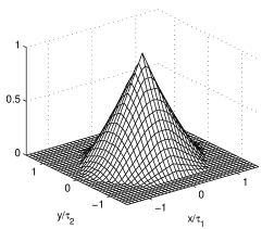
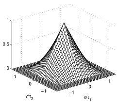
Figure 13: Convolution of two hexagons of an array with $\tau_{1}=\tau_{2}$ (left). Convolution of two rectangles (right). The first type of crosstalk eliminates the COG discretization error for any array of detectors with $\tau_{1}=\tau_{2}$ and $\alpha=2$; the second eliminates it even for any $\alpha$.

Figure 13 shows two forms of crosstalk. We can see that the convolution of two constant height hexagonal surface generates a surface with negligible edges much resembling a cone. The base is always hexagonal. In the convolution of two constant height square surfaces, two edges are present. If the two convolved forms are both sized $\tau_{1}$x$\,\tau_{2}$, their convolution is $2\tau_{1}$x$\,2\tau_{2}$. These are the smallest sizes. The convolution of any crosstalk function free of discretization error with any normalized function saves the property, but the size of the resulting function is the sum of the sizes of the two convolved functions.

With a set of steps giving Eq. (9), it can be proved that any function g$(x,y)$ with the following property is free of the COG discretization error for $x_{g}$ and for $y_{g}$:

$$\sum_{n,l=-\infty}^{+\infty}(n\tau_{1}+\frac{l\tau_{2}}{\alpha}-x)\ \mathrm{g}(n\tau_{1}+\frac{l\tau_{2}}{\alpha}-x;l\tau_{2}-y)=0\ \ \ (\text{a.\ e.})$$ (40)

$$\sum_{n,l=-\infty}^{+\infty}(l\tau_{2}-y)\ \mathrm{g}(n\tau_{1}+\frac{l\tau_{2}}{\alpha}-x;l\tau_{2}-y)=0\ \ \ \ \ \quad\quad (\text{a.\ e.})\ .$$

We are unable to give an example of detectors which implement or attempt to approach this feature. In the one-dimensional case, the silicon strip detector with floating strips probably approaches a crosstalk which tends to a form free of discretization error for any signal distribution.

It is useful to discuss the criticality of condition (40) in the presence of a size (or period) mismatch. For this,

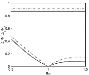
Figure 14: Effects of the crosstalk on a pair of near $\delta$-like signals. The upper curves are $\Delta_{x_{g}}$ and $\Delta_{y_{g}}$ for a square array without crosstalk. The lower curves are given by the presence of a square crosstalk and ranges running from $R/\tau=0.5$ up to $R/\tau=1.5$. For $R/\tau=1$, the error is completely suppressed.

we construct a simulation with a narrow signal distribution and a large discretization error on an array with $\tau_{1}=\tau_{2}=1$, and a crosstalk function dimensioned around the optimal value. A dramatic improvement — even for large discrepancies with respect to the exact value — can be seen in Fig. 14. The crosstalk is a square of varying dimensions. This form is probably of interest for the pixel detector of CMS [12], but it is impractical for homogeneous detectors where axisymmetric shapes are more probable. The smallest size axisymmetric crosstalk which heavily suppresses the COG discretization error is the disk of $R/\tau\approx 1.2$ due to the first zero of J${}_{1}(\omega)$ FT of a disk (in this case g$(x,y)$ has a range of $2.2\tau$). Even if this is not an exact suppression, it looks very efficient and almost independent of $\alpha$, at least for large (or small) $\alpha$ values.

Another approximate suppression of the COG error is given by the conoid form of the crosstalk, which is obtained by the convolution of two disks. Here the overlap of the zeros of J${}_{1}(\omega)^{2}$ almost completely suppresses the COG error beyond $R/\tau\approx 2$. Axial symmetry is granted even in this case, and the insensibility to the $\alpha$ values is more pronounced than in the case of a disk. On the basis of these considerations, Fig. 4 can be read as the effects of various types of crosstalk on a $\delta$-like signal distribution.

7 Finite Array of Detectors

7.1 Imaging on a Pixel Detector

Up to now, we have explored an infinite periodic array of detectors, and the sampling-function periodicity was the key property in extracting explicit analytical results. With a finite set of detectors, periodicity disappears and calculation of the convolutions is unavoidable. But, as proved in Ref. [1], the solution to the problem lies in the finite range of the signal distribution $\varphi(\mathbf{x})$ and the limited number of detectors ($2$x$3,\ 3$x$3,\ 5$x$5,\dots$). Without losing the locality property of $\mathbf{r}_{g}$, we can use a periodic repetition of $\varphi(\mathbf{x})$ (indicated with $\varphi^{p}(\mathbf{x})$) or the periodic repetition of the set of detectors. Since the second looks more involved analytically, we will use the first approach. The periodic $\varphi^{p}(\mathbf{x})$ explores the set of detectors, and if the periods are sufficiently ample, the (periodic) convolution with the sensor function g$(\mathbf{x})$ coincides with the convolution of $\varphi(\mathbf{x})$ on a period. As in [1], the periodic function $\varphi^{p}(\mathbf{x})$ with periods $T_{1}$ and $T_{2}$ is defined as (for $\,r,s\in\mathbb{Z}^{2}$ and with the vectors $\mathbf{T}_{1}=(T_{1}\,;\,0)$, and $\mathbf{T}_{2}=(0\,;\,T_{2})$):

$$\varphi^{p}(\mathbf{x})=\sum_{r,s}\varphi(\mathbf{x}-r\mathbf{T}_{1}-s\mathbf{T}_{2})\,.$$

The FT of $\varphi^{p}(\mathbf{x})$ (indicated with $\Phi^{p}(\boldsymbol{\omega})$) has components at frequencies that are multiples of the fundamental frequencies $2\pi/T_{1}$ and $2\pi/T_{2}$ and introducing the vectors $\mathbf{R}_{1}=(2\pi/T_{1}\,;\,0)$ and $\mathbf{R}_{2}=(0\,;\,2\pi/T_{2})$:

$$\Phi^{p}(\boldsymbol{\omega})=\frac{(2\pi)^{2}}{T_{1}T_{2}}\sum_{m,k}\delta(\boldsymbol{\omega}-m\mathbf{R}_{1}-k\mathbf{R}_{2})\,\Phi(m\,R_{1};k\,R_{2}),$$ (41)

where the amplitudes $\Phi(m\,R_{1};k\,R_{2})$ are the values of the FT of $\varphi(\mathbf{x})$ taken at the corresponding values. We will assume that $T_{1}$ and $T_{2}$ are larger than the region involved in the sampling (i.e., the set of sensors are well contained in a rectangle $T_{1}$x$T_{2}$), so we can write:

$$\mathrm{f}^{p}(n\mathbf{n}_{1}+l\mathbf{n}_{2}-\boldsymbol{\varepsilon})=\mathrm{f}(n\mathbf{n}_{1}+l\mathbf{n}_{2}-\boldsymbol{\varepsilon})\ \ \ \text{n,l}\ \epsilon\ I_{0}\ \ \ \varepsilon_{1},\varepsilon_{2}\ \epsilon\ C_{1}\,.$$

$$\mathrm{f}^{p}(\mathbf{x})=\sum_{m,k}\mathrm{e}^{i(m\,\mathbf{R}_{1}+k\,\mathbf{R}_{2})\cdot\,\mathbf{x}}\mathrm{G}(mR_{1}\,;\,kR_{2})\Phi(mR_{1}\,;kR_{2})\frac{1}{T_{1}T_{2}}\,.$$

Now, the set $I_{0}$ of the detector indexes $n$ and $l$ is some subset of integers and $\boldsymbol{\varepsilon}$ covers a detector. We define a function s${}^{p}_{\boldsymbol{\varepsilon}}(\mathbf{x})$ as:

$$\mathrm{s}^{p}_{\boldsymbol{\varepsilon}}(\mathbf{x})=\sum_{n,l\,\in\,I_{0}}\delta(\mathbf{x}-n\mathbf{n}_{1}-l\mathbf{n}_{2})\,\mathrm{f}^{p}(\mathbf{x}-\boldsymbol{\varepsilon})$$

where s${}^{p}_{\boldsymbol{\varepsilon}}(\mathbf{x})$ is expressed as sum of products of two $\mathbf{x}$-functions. The FT of s${}^{p}_{\boldsymbol{\varepsilon}}(\mathbf{x})$ is the convolution of the FTs of the two functions. However, f${}^{p}(\mathbf{x})$ is periodic and has a FT similar to that of Eq. (41). This eliminates the integrations in the convolution and blocks the integration variables to the values of their $\delta$-functions. Then, S${}^{p}_{\boldsymbol{\varepsilon}}(\boldsymbol{\omega})$ becomes:

$$\mathrm{S}^{p}_{\boldsymbol{\varepsilon}}(\boldsymbol{\omega})= \int_{\mathbb{R}^{2}}\frac{d\boldsymbol{\omega}}{4\pi^{2}}\mathrm{H}(\boldsymbol{\omega}-\boldsymbol{\omega}^{\prime})\mathrm{F}^{p}(\boldsymbol{\omega}^{\prime})$$ (42)

$$\mathrm{S}^{p}_{\boldsymbol{\varepsilon}}(\boldsymbol{\omega})= \frac{1}{T_{1}T_{2}}\sum_{m,k\,\in\,\mathbb{Z}^{2}}\ \sum_{n,l\,\in\,I_{0}}\mathrm{e}^{-i(n\mathbf{n}_{1}+l\mathbf{n}_{2})(\boldsymbol{\omega}-m\mathbf{R}_{1}-k\mathbf{R}_{2})}$$

$$\mathrm{e}^{-i(m\mathbf{R}_{1}+k\mathbf{R}_{2})\cdot\,\boldsymbol{\varepsilon}}\mathrm{G}(mR_{1};kR_{2})\Phi(mR_{1};kR_{2})\ ,$$

where H$(\boldsymbol{\omega})$ is the FT of the set of Dirac $\delta$-functions that define the detector positions.

Applying Eqs. (18) to Eq. (42), we can calculate the two components of $\mathbf{r}_{g}$. These equations can be easily generalized to a finite array of different detectors as the type discussed in [15], or to a subset of detectors of Penrose tessellation [5]. Each type of detector is introduced with its proper (different) f${}^{p}_{n,l}(\mathbf{x})$ produced by a g${}_{n,l}(\mathbf{x})$ function convolving the same signal distribution. The g${}_{n,l}(\mathbf{x})$ functions account for the properties of the detectors located in the points labelled by the indexes $\{n,l\}$. Then, we must modify Eq. (42) accordingly, introducing functions G${}_{n,l}(\boldsymbol{\omega})$, FT of g${}_{n,l}(\mathbf{x})$, that contain the shape, efficiency etc. of the detectors with their COGs in position $\{x_{n},y_{l}\}$.

7.2 3x3 and 5x5 Detector Arrays

Let us describe the $3$x$3$ and $5$x$5$ arrays of rectangular detectors of the same type. In Eq. (42), the two sets of indexes $n$ and $l$ run on the integers $\{-1,\ 0,\ 1\}$, for the $3$x$3$ array, and $\{-2,-1,\ 0,\ 1,\ 2\}$ for the $5$x$5$. H${}^{5\mathrm{x}5}(\boldsymbol{\omega})$ and H${}^{3\mathrm{x}3}(\boldsymbol{\omega})$ becomes:

$$\mathrm{H}^{5\mathrm{x}5}(\boldsymbol{\omega})= [2\cos(2\omega_{x}\tau_{1})+2\cos(2\omega_{x}\tau_{1})+1][2\cos(2\omega_{y}\tau_{2})+2\cos(2\omega_{y}\tau_{2})+1]$$ (43)

$$\mathrm{H}^{3\mathrm{x}3}(\boldsymbol{\omega})= [2\cos(2\omega_{x}\tau_{1})+1][2\cos(2\omega_{y}\tau_{2})+1]$$

and $x_{g}$ for a $3$x$3$ array becomes:

$$x^{3\mathrm{x}3}_{g}=\frac{i}{T_{1}T_{2}}\sum_{m,k} 2\tau_{1}\sin(mR_{1}\tau_{1})\big{[}2\cos(kR_{2}\tau_{2})+1\big{]}\,\mathrm{e}^{-i(m\mathbf{R}_{1}+k\mathbf{R}_{2})\,\cdot\,\boldsymbol{\varepsilon}}\,$$ (44)

$$\mathrm{G}(mR_{1};kR_{2})\,\Phi(mR_{1};kR_{2})\,.$$

Similar expressions can be easily obtained for $y_{g}$ and for a $5$x$5$ array. As discussed in [1], a set of discontinuities are present in $\mathbf{r}_{g}(\boldsymbol{\varepsilon})$ if the signal distribution extends beyond the limits of the array. In both cases, the discontinuities are located at the borders of the central detector. Near the borders, the suppressed tails of the signal distributions tend to differ, thereby inducing an error in the COGs. Beyond the borders, a different set of detectors are inserted in the algorithm, and the error changes sign, generating a

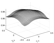
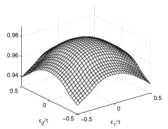
Figure 15: The surface on the left is the efficiency for energy collection of the $5$x$5$ algorithm (i.e., S${}^{5\mathrm{x}5}(0,0)$). The surface on the right is the efficiency of the $3$x$3$ algorithm (S${}^{3\mathrm{x}3}(0,0)$).

discontinuity.

To show how the $3$x$3$ and $5$x$5$ algorithms work, we will apply them to a detector similar to the CMS em calorimeter [13] with a signal distribution generated as described in [1] for a set of tracks. In [1], we explored the form of the average signal distribution generated by a set of random tracks whose parameters where tuned to reproduce the average lateral signal distribution of an em shower as extracted from the data in Ref. [14]. The shower’s axis is parallel to the detector’s $z$-axis, so the tracks’ useful parameters do not contain their $z$-origin. In the CMS em calorimeter, the crystals have a nonprojective geometry with a $3^{\circ}$x$\,3^{\circ}$ off-center pointing. In the simulation the shower axis is bent respect to the detector’s $z$-axis, and the longitudinal distribution of the track origins must be introduced. This can be produced by adding a $z$-dependent probability distribution of the track origins whose average reproduces the average longitudinal energy distribution of a $200$ GeV photon-shower as parameterized in [16]. The set of tracks are globally bent $3^{\circ}$ in $y$- and in $x$-direction to simulate the off-axis distortion of the CMS-crystals. The average over $150$ distributions is used to calculate the efficiency surfaces of the $5$x$5$ and $3$x$3$ energy reconstruction algorithms. It should be stressed that this is not a Monte Carlo simulation, but a toy model that allows easy calculation of S${}^{5\mathrm{x}5}(0,0)$ and S${}^{3\mathrm{x}3}(0,0)$. Most likely, the average signal distribution is realistic enough for our needs: In fact, the signal distribution is filtered by a low-pass filter and very few details are relevant to this simulation.

The bending of the em-shower axis renders the signal distribution slightly asymmetric. The COG shower does not coincide with the impact point of the photon on the face of the central crystal. To reconstruct the impact point, further assumptions are required. Our natural reference point is the COG signal distribution, which sets the maximum of the efficiency plots in the center of the detector. The range of allowed $\boldsymbol{\varepsilon}$-values is limited by the central-detector boundaries.

Figure 15 shows the efficiency plots of algorithms $5$x$5$ and $3$x$3$. There is evidently greater signal loss and greater suppression of the signal tails in the $3$x$3$ array. The marked reductions at the borders of the $5$x$5$ array are due to the loss at the boundaries between crystals. This loss is simulated as a dead space whose length is the fraction of effective radiation length of the interspersed material. In these plots, we neglect an effect of the asymmetry of the signal distribution that, at a pair of corners, moves the maximum collected energy on a nearby crystal not containing the COG shower.

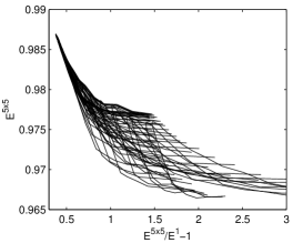
Figure 16: Energy collected by the 5x5 array E$\,{}^{5x5}$in function of the quantity E$\,{}^{5x5}/$E${}^{1}-1$. This plot cannot be reduced to a line as is usually done for the energy reconstruction.

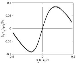
Figure 17: Set of plots for various values of $\varepsilon_{2}$ of COG error $\varepsilon_{1}-x_{g}$, each shown in function of $x_{g}$.

The efficiency surfaces of Fig. 15 show a decrease at the borders. The decrease is usually recovered by ad hoc reconstruction methods. One method [13] is to consider the plot of E$\,{}^{5\mathrm{x}5}$ in relation to E$\,{}^{5\mathrm{x}5}$/E${}^{1}-1$ and fit the resulting distribution (E¹ is the energy collected by the central detector). It is evident from Fig. 16 that this function cannot be fit to a line without introducing an effective broadening of the energy resolution. The functions E^5x5 and E¹ are surfaces and have a complex correspondence. It is our guess that accounting for them could improve the energy reconstruction.

The COG error $(\varepsilon_{1}-x_{g})$ in relation to $x_{g}$ is illustrated in Fig. 17 for an array of $3$x$3$ detectors. This quantity is a function of $\varepsilon_{1}$ and $\varepsilon_{2}$, but, contrary to expectations, the dependence on $\varepsilon_{2}$ is negligible. This almost decoupling of the $x_{g}$ error from $\varepsilon_{2}$ and $y_{g}$ error from $\varepsilon_{1}$ allows each error to be corrected independently with the methods discussed in [1]. A slight dependence of $x_{g}$ on $\varepsilon_{2}$ is probably introduced by the border regions where the maximum signal detector is not that containing the COG shower. These regions are at the corners of the central detector, where the signal spreads almost evenly over four detectors, and the COG error is very small.

7.3 Triangular Detectors

This subsection is devoted to describe the energy and position reconstructions in the Crystal Ball (CB) detector [2], a first-generation em calorimeter still in operation at the BNL [17] which is applied to the study of barionic resonances. This application illustrates the effectiveness of Eqs. (41,42) to a complex geometry such as that of the CB. As mentioned in Section 3.3, the CB calorimeter is composed of 672 optically isolated NaI(Tl) crystals. Each crystal is shaped as a truncated triangular pyramid, 40.6 cm long, pointing toward the interaction point, with 5.1 cm sides at the inner end and 12.7 cm sides at the outer end. The crystal setup is based on the geometry of an icosahedron having an equatorial plane that allows the separation of the ball into two hemispheres for easily opening. Each of the twenty main triangular faces of the icosahedron ($major\ triangles$) is divided into four $minor\ triangles$, each one consisting of nine individual crystals. Some crystals are removed at two sides of the equatorial plane to make room for the beam pipe.

Some details are ignored in the simulation. Having to work on a plane, we project a restricted set of triangular detectors. The significant differences in size of the top and bottom are neglected; each detector’s size will be that measured at the shower maximum ($40$ cm from the center of the CB for electron showers and $0.8$ radiation lengths more for photon showers). The energy reconstruction algorithm (as used long ago in the CB experiment in DESY at the DORIS II accelerator [18]) sums all the energy released in 12 crystals around the crystal with the maximum energy of the cluster and the maximum itself (E₁₃).

The triangles’ relative positions in the array are crucial. The $n$ and $l$ values for the downward triangles to be used in Eq. (42) are: $[(0,1)$ $(-1,1)$ $(-1,0)$ $(0,0)$ $(1,0)$ $(0,-1)$ $(1,-1)]$. The upward triangles have $n$ and $l$ given by: $[(-1,0)$ $(0,0)$ $(1,0)$ $(0,-1)$ $(1,-1)$ $(1,-2)]$. It should be recalled that the origin of the sampling for the upward triangles is shifted by $2\,\tau_{2}/3$ and $\alpha$ is $2\,\tau_{2}/\tau_{1}$. The triangles are equilateral with $\tau_{1}=3.37$ radiation lengths and high $\tau_{2}$. Using Eq. (12) in Eq. (42), we obtain $\mathbf{r}_{g}(\boldsymbol{\varepsilon})$. Due to the lack of symmetry, we must carefully account for the relative phases of the complex quantities involved.

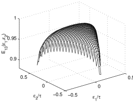
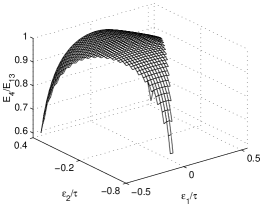
Figure 18: The surface on the left is S${}_{\varepsilon_{1},\varepsilon_{2}}(0,0)$ for the array of 13 crystals. $\varepsilon_{1}$ and $\varepsilon_{2}$ explore the central crystal. The surface on the right is the ration E${}_{4}/$E₁₃. Here, the efficiency drop at the borders of a crystal disappears, while the drop at the corners increases.

We apply Eqs. (41,42) to the set of triangles, remembering the differences of the upward and downward triangles as discussed in Section 3.3. We must use Eq. (29) in Eq. (42) for the upward triangles and its complex conjugate for the downward triangles. The average signal distribution is the model distribution generated as described in [1] to reproduce the lateral signal distribution of an em shower. Here no $z$-distribution of the tracks is needed due to the coincidence of the CB center with the interaction point (projective geometry). The loss at the crystal borders is probably underestimated, since the model assumes that all the photons convert. Theoretically, the projective geometry allows photons to escape detection with an efficiency dropping near zero.

The efficiency plot in Fig. 18 is calculated for the range of $\boldsymbol{\varepsilon}$-value covering the central triangle. As expected, the plot is a surface, and surfaces are the ratios with other partial sums of the collected energy. For example, histograms of E${}_{4}/$E₁₃ were used in cuts to reduce the $\pi_{0}$ contamination, where E₄ is the energy collected by the central crystal and by its three nearest ones. Even if our simulation of E${}_{4}/$E₁₃ recovers the drop in signal collection caused by the loss at the crystal borders, it is unable to recover the signal spread in neighboring crystals. Therefore, dealing with these distributions as parameters, effective broadening due to geometrical effects is introduced in the reconstructions, and good events are eliminated.

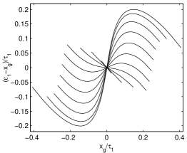
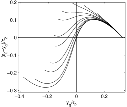
Figure 19: The COG error $(\varepsilon_{1}-x_{g})$ in function of $x_{g}$ (left), each curve plots a specific $\varepsilon_{2}$-value. The COG error $\varepsilon_{2}-y_{g}$ in function of $y_{g}$ (right), each curve plots a specific $\varepsilon_{1}$-value.

The COG error in CB, as shown in Fig. 19, is very large, and without correction, errors of the order of $\tau_{1}/4$ are often encountered. This is due to the very narrow core of our—very realistic—shower model that concentrates a large fraction of signal in the central crystal. The plots in Fig. 19 are rounded at the borders due to the signal collected by the lateral detectors, and the range of $x_{g}$-values covers almost all the central detector. In contrast to Fig. 17, $(\varepsilon_{1}-x_{g})$ has a strong dependence on $\varepsilon_{1}$ and $\varepsilon_{2}$, and, similarly $(\varepsilon_{2}-y_{g})$. It is evident that the correction of these COG errors is a very complex operation, and the programs developed by CB collaboration were accordingly complex.

This example illustrates one of the more complicated cases, but the application of our equations is not more involved than the case of an array of square detectors. The equations and considerations in Section 3.3 are crucial to rapidly generate the simulation.

8 Conclusions

The COG error calculation for a two-dimensional array of sensors has been explored in detail. All the relevant equations have been discussed to allow safe applications with similar or different systems. This approach generalizes the results of [1], with the evident complexity of the two-dimensional geometry. All the equations contain double infinite sums and look very involved. The sums converge rapidly and a fairly limited number of terms are required to get satisfactory results; the applications and figures presented were obtained with only a few lines of MATLAB [19] code.

Forms of crosstalk which save the signal collection efficiency, and those in which the COG algorithm is free of discretization errors for any form of signal distributions may be isolated. The set of special forms is now much larger than in the one-dimensional case. These properties are collected in easily verifiable conditions on the function g$(\mathbf{x})$.

The set of properties of the g$(\mathbf{x})$-functions without crosstalk made it possible to prove that orthogonal and complete bases can be extracted from their Fourier transforms, giving a nonseparable two-dimensional form of the Wittaker-Kotel’nikov-Shannon theorem.

A type of crosstalk, which turned out to be largely independent of the shape and periodicity of the array, was detected. This crosstalk only generates an approximate cancellation of the COG discretization error for any signal distribution. The effect is given by the first zero of the J₁-Bessel function which suppresses the first element of the COG error series. The fast decrease with the frequency of the Fourier-Series terms forming the COG error assigns an important contribution to the first term. The remaining terms contribute only slightly to the total COG-error. Not being exact, the result must be tested for the specific problem, but from the structure of the terms forming the COG errors, it can be inferred that the error reduction is substantial for any signal distribution.

To prove the previous general (or approximate) results, we worked with an infinite array of identical detectors, these equations can be used for detector optimizations.

In the experiments, reconstructions with a selection of detectors is a standard procedure to reduce the noise. To study the effects of these selections, we developed methods to handle a finite set of detectors. It is evident that the exact results are only of approximate validity in these cases. If the crosstalk completely suppresses the COG discretization error for any signal distribution in an infinite array, the suppression could not be complete for a finite set of detectors and could be (slightly) dependent upon the signal distribution.

The simulation of the energy reconstruction in an em-calorimeter such that of the CMS experiment highlights a position dependence of the reconstruction efficiency. This dependence does not appear to be recoverable using the standard tools for extracting parameters from ratios of signal collected by a different number of detectors. The $\boldsymbol{\varepsilon}$-dependence of these ratios does not allow their use as parameters. The fluctuations of the Monte Carlo simulations cover the distribution of their mean values due to the shower position.

References

- [1] G. Landi, Nucl. Instr. and Meth. A 485 (2002) 698 (also arXiv:1908.04447).
- [2] E.D. Bloom and C.W. Peck, Annu. Rev. Nucl. Part. Sci. 33 (1983) 143.
- [3] R.N. Bracewell, The Fourier Transform and Its Application. (McGraw-Hill, New York, NY, 1986).
- [4] M.C. Escher, J.W. Vermeulen, Escher on Escher: Exploring the Infinite. (H.N.Adams. New York, NY, 1989).
- [5] R. Penrose, The Emperor’s New Mind: Concerning Computers, Minds, and the Laws of Physics. (Oxford University Press, Oxford, UK, 1989)
- [6] D.C. Champeney, A Handbook of Fourier Theorems. (Cambridge University Press, Cambridge, UK, 1987).
- [7] B.V. Delft Electronische Producten, Roden, The Netherlands.
- [8] MATHEMATICA 3. Wolfram Research, Inc.
- [9] H. Dym, H.P. McKean, Fourier Series and Integrals. (Academic Press, London, 1972).
-
[10]
A.J. Jerri, Proceedings IEEE 65, 1565 (1977).
J.M. Whittaker, Proc. Math. Soc. 1, 169 (1929).
V.A. Kotel’nikov, Izd. Red. Upr. Svyazi RKKA (Moscow, URSS, 1933).
C.E. Shannon, Proc. IRE 37, 10 (1949). - [11] S. Mallat, A Wavelet Tour of Signal Processing. (Academic Press, London, UK, 1999).
- [12] CMS. The Tracker Project. TDR. CERN/LHCC 98-3.
- [13] CMS. The Electromagnetic Calorimeter. TDR. CERN/LHCC 97-33.
- [14] A.A. Lednev, Nucl. Instr. Meth. A 366, 298 (1995).
- [15] S. Hillert et. al., Nucl. Instr. Meth. A 458, 710 (2001).
- [16] E. Longo and I. Sestili, Nucl. Instr. Meth. 128, 283 (1975).
- [17] T.D.S. Stanislaus et al., Nucl. Instr. Meth. A 462, 463 (2001).
- [18] D. Antreasyan et al., Z. Phys. C 48, 553 (1990).
- [19] MATLAB 6.1, The MathWorks, Inc.