Density ratio model with data-adaptive basis function

Abstract

In many applications, we collect independent samples from interconnected populations. These population distributions share some latent structure, so it is advantageous to jointly analyze the samples. One effective way to connect the distributions is the semiparametric density ratio model (DRM). A key ingredient in the DRM is that the log density ratios are linear combinations of prespecified functions; the vector formed by these functions is called the basis function. A sensible basis function can often be chosen based on knowledge of the context, and DRM-based inference is effective even if the basis function is imperfect. However, a data-adaptive approach to the choice of basis function remains an interesting and important research problem. We propose an approach based on the classical functional principal component analysis (FPCA). Under some conditions, we show that this approach leads to consistent basis function estimation. Our simulation results show that the proposed adaptive choice leads to an efficiency gain. We use a real-data example to demonstrate the efficiency gain and the ease of our approach.

Keywords: Density estimation; Empirical likelihood; Functional principal component analysis; Multiple samples; Quantile estimation.

1 Introduction

This research is motivated by applications where multiple samples are collected from connected or similar populations. For example, the income distribution of individuals or households is a key economic indicator for a country. Economists are keenly interested in changes over time in income distributions. One may postulate a parametric model for these distributions, but a mild violation of the model assumptions may lead to dubious conclusions. Nonparametric approaches avoid such risks, at the cost of statistical efficiency. Semiparametric approaches offer a middle ground. Chen and Liu (2013) propose connecting the population distributions via the density ratio model (DRM) of Anderson (1979). Specifically, let the population distributions be $G_{k}(\cdot)$ for population $k=0,\ldots,m$, and let their respective density functions with respect to some $\sigma$-finite measure be $g_{k}(\cdot)$. The DRM postulates that

$$g_{k}(x)=g_{0}(x)\exp\{\alpha_{k}+\bm{\beta}_{k}^{\top}\bm{\mathrm{q}}(x)\},\hskip 14.22636ptk=1,\ldots,m,$$ (1)

for some known vector-valued basis function $\bm{\mathrm{q}}(\cdot)$ and unknown parameters $(\alpha_{k},\bm{\beta}_{k})$. We refer to distribution $G_{0}(\cdot)$ as the base distribution, but any $G_{k}(\cdot)$ could serve the same purpose. The DRM is closely connected with other semiparametric models such as the biased sampling model (Vardi, 1982, 1985; Qin, 2017), the exponential tilting model (Rathouz and Gao, 2009), and the proportional likelihood ratio model (Luo and Tsai, 2012). The DRM characterizes the common features of the multiple populations through the basis function $\bm{\mathrm{q}}(\cdot)$. There have been many interesting developments in inference under the DRM (Qin, 1993; Qin and Zhang, 1997; Fokianos et al., 2001; Qin, 1998; Chen and Liu, 2013; Cai et al., 2017; De Oliveira and Kedem, 2017; Sugiyama et al., 2012). The model has been adopted in a broad range of applications, including time series (Kedem et al., 2008), finite mixture models (Tan, 2009; Li et al., 2017), mean regression models (Huang and Rathouz, 2012), the detection of changes in lower percentiles (Chen et al., 2016), and the study of dominance relationships among multiple populations (Zhuang et al., 2019).

There has been much interest in both theory and methodological developments, and one challenging research problem is the choice of $\bm{\mathrm{q}}(\cdot)$. The existing results are usually obtained under the assumption that $\bm{\mathrm{q}}(\cdot)$ is correctly specified. There are also natural choices that lead to reliable inference conclusions. For example, one may set $\bm{\mathrm{q}}(x)=(x,x^{2})^{\top}$ when the data histograms resemble those of normal densities or use $\bm{\mathrm{q}}(x)=(|x|^{1/2},x,x^{2},\log(1+|x|))^{\top}$ to cover a large territory. Fokianos (2007) proposes choosing the basis function via selection criteria, such as the Akaike information criterion (AIC; Akaike, 1973) or the Bayesian information criterion (BIC; Schwarz, 1978). Chen and Liu (2013) suggest that if the basis function is rich but not perfect, empirical-likelihood-based quantile estimators are still more efficient than the sample quantiles. However, in some applications model misspecification is still an issue. Fokianos and Kaimi (2006) and Fokianos (2007) report increased bias in the estimation of model parameters and power loss in hypothesis tests if the basis function is underfitted, overfitted, or misspecified. An adaptive basis function can be useful in such situations.

In this paper, we propose an approach based on functional principal component analysis (FPCA; Ramsay and Silverman, 2005; Wang et al., 2016). FPCA identifies variability and similarity among the functions of interest through an “optimal” expansion of these functions. Accurate approximations can be obtained by linear combinations of a few eigenfunctions. For the DRM, we identify the most important eigenfunctions of the log density ratios $\{\log(g_{k}(x)/g_{0}(x)):k=0,\ldots,m\}$ through multiple samples and thus obtain a data-adaptive $\bm{\mathrm{q}}(\cdot)$. Under the assumption that the log density ratios belong to a low-dimensional space, the proposed estimators are consistent. Our simulation experiments show that when the data are generated from commonly used distributions, DRM analysis based on an adaptive basis function has a promising efficiency. In fact, it is often comparable with an analysis based on the “most suitable” basis function. Naturally, if the natural basis function for a multiple-sample dataset is unsuitable, the adaptive choice has a superior performance. Our real-data example confirms this finding.

2 Basis functions for DRM and FPCA

2.1 Overview of DRM

Let $\{x_{kj}:j=1,\ldots,n_{k};k=0,\ldots,m\}$ be $m+1$ independent samples, each consisting of independent and identically distributed (i.i.d.) observations from a distribution $G_{k}$. We assume that the population distributions $G_{k}$ satisfy the DRM as given in (1). However, we do not assume knowledge of the basis function $\bm{\mathrm{q}}(\cdot)$. Let $N=n_{0}+\cdots+n_{m}$. We propose a data-adaptive choice of $\bm{\mathrm{q}}(\cdot)$ under the assumption that $\rho_{k}=n_{k}/N$ has a nonzero limit for each $k$ as $N\to\infty$, while $m$ is constant. Without loss of generality, we will regard $\rho_{k}$ as a constant not evolving with $N$. This is sensible because the asymptotic results apply when $N$ is large and the proportions $\rho_{k}$ are not too close to zero. How the inference evolves with $N$ is not an issue in applications. With this understanding, we define

$$\bar{G}(x)=\sum_{k=0}^{m}\rho_{k}G_{k}(x)$$

to be a mixture distribution by regarding the $G_{k}(\cdot)$ as subpopulation distributions. Let $X$ be a generic random variable. We denote

$$\bar{E}\{h(X)\}=\int h(x)\mathrm{d}\bar{G}(x)$$

whenever the integration is well defined, for a generic function $h(\cdot)$. Next, we assume that the unknown vector-valued basis function satisfies $\bar{E}\{\bm{\mathrm{q}}(X)\}=\bm{0}.$ If it does not, we can write

$$\alpha_{k}+\bm{\beta}^{\top}\bm{\mathrm{q}}(x)=\alpha_{k}+\bm{\beta}^{\top}\bar{E}\{\bm{\mathrm{q}}(X)\}+\bm{\beta}^{\top}\big{[}\bm{\mathrm{q}}(x)-\bar{E}\{\bm{\mathrm{q}}(X)\}\big{]}$$

and replace $\bm{\mathrm{q}}(\cdot)$ by $\bm{\mathrm{q}}(\cdot)-\bar{E}\{\bm{\mathrm{q}}(X)\}$ to ensure that the assumption is satisfied when the expectation is finite.

After we obtain a data-adaptive choice of $\bm{\mathrm{q}}(\cdot)$, we will reuse the data to fit the DRM (1) to estimate $(\alpha_{k},\bm{\beta}_{k})$ based on the empirical likelihood; see $\S$ 5.1. We first need some FPCA theory.

2.2 Functional principal component analysis

Let $T$ be a closed subset of $\mathbb{R}$, $\mathscr{B}(T)$ the Borel $\sigma$-algebra on $T$, and ${\mathcal{M}}$ a probability measure, such that $(T,\mathscr{B}(T),{\mathcal{M}})$ forms a measure space. Let $L^{2}(T,{\mathcal{M}})$ be the space of all measurable real-valued functions on $T$ such that $\int_{T}f(t){\mathcal{M}}(\mathrm{d}t)=0$ and $\int_{T}f^{2}(t){\mathcal{M}}(\mathrm{d}t)<\infty.$ With ${\mathcal{M}}$ a probability measure, all square integrable functions can be centralized. Hence, we have not excluded many functions from the usual $L^{2}(T,{\mathcal{M}})$ space. For any $f,g\in L^{2}(T,{\mathcal{M}})$, define the inner product to be

$$\langle f,g\rangle=\int_{T}f(t)g(t){\mathcal{M}}(\mathrm{d}t).$$

According to the comment after Definition 1.6 of Conway (2007), $L^{2}(T,{\mathcal{M}})$ is a Hilbert space with norm $\|f\|_{2}=(\langle f,f\rangle)^{1/2}$.

Let $\Sigma(s,t)$ be a symmetric, nonnegative definite, and square integrable function with respect to ${\mathcal{M}}$, such that $\int_{T}\int_{T}\Sigma^{2}(s,t){\mathcal{M}}(\mathrm{d}s){\mathcal{M}}(\mathrm{d}t)<\infty,$ and for any $s,t\in T$, $\int\Sigma(s,t){\mathcal{M}}(\mathrm{d}s)=\int\Sigma(s,t){\mathcal{M}}(\mathrm{d}t)=0.$ For instance, $\Sigma(s,t)=(s-c)(t-c)$ with $c=\int t{\mathcal{M}}(\mathrm{d}t)$ is such a bivariate function when ${\mathcal{M}}$ has a finite second moment. Next, we define a Hilbert–Schmidt integral operator ${\mathcal{V}}$ (Arveson, 2006) as

$$[\mathcal{V}f](t)=\int_{T}\Sigma(s,t)f(s){\mathcal{M}}(\mathrm{d}s),$$ (2)

for any function $f\in L^{2}(T,{\mathcal{M}})$. It can be seen that $[\mathcal{V}f](t)\in L^{2}(T,{\mathcal{M}})$.

In the context of the DRM, let $q_{1}(\cdot),\ldots,q_{d}(\cdot)$ be $d$ distinct and orthonormal functions in $L^{2}(T,{\mathcal{M}})$. Let $\Sigma(s,t)=\sum_{j=1}^{d}\lambda_{j}q_{j}(s)q_{j}(t)$ for some positive values $\lambda_{1},\ldots,\lambda_{d}$. Clearly, its Hilbert–Schmidt integral operator ${\mathcal{V}}$ has $\{\lambda_{j},q_{j}(t)\}_{j=1}^{d}$ as its eigenvalues and eigenfunctions. Further, $[\mathcal{V}f](t)$ is always a linear combination of $\{q_{j}(t)\}_{j=1}^{d}$. Hence, ${\mathcal{V}}$ has no other nonzero eigenvalues. By the spectral theorem, any $f\in L^{2}(T,{\mathcal{M}})$ can be decomposed as $f(t)=\sum_{j=1}^{d}a_{j}q_{j}(t)+h(t),$ for some $h(t)$ such that $[\mathcal{V}h](t)=0$, and $a_{j}=\langle f,q_{j}\rangle$.

2.3 Applying FPCA to DRM

We now revise the DRM assumption so that the meaning of the notation in (1) aligns with that in $\S$ 2.2. Let ${\mathcal{X}}$ be the common support of population distributions $\{G_{k}(\cdot):k=0,\ldots,m\}$. We assume that there exist $d<m$ distinct and orthonormal functions $q_{1}(\cdot),\ldots,q_{d}(\cdot)$ of $L^{2}({\mathcal{X}},\bar{G})$ and unknown parameters in the form $(\alpha_{k},\bm{\beta}_{k})$ such that

$$Q_{k}(x)=\log\{g_{k}(x)/g_{0}(x)\}=\alpha_{k}+\bm{\beta}_{k}^{\top}\bm{\mathrm{q}}(x),$$

for $k=0,\ldots,m$, where $(\alpha_{0},\bm{\beta}_{0})=\bm{0}$ and $\bm{\mathrm{q}}(x)=(q_{1}(x),\ldots,q_{d}(x))^{\top}$.

By the Gram–Schmidt orthogonalization process (Conway, 2007), the existence of $\bm{\mathrm{q}}(\cdot)$ with these properties is guaranteed. We have required only that $\bm{\mathrm{q}}(\cdot)$ is square integrable with respect to $\bar{G}$. This condition imposes a minimum restriction on the DRM: the second moment of $\bm{\mathrm{q}}(X)$ must be finite. We hope that $d<m$ so that the DRM itself is meaningful in applications. For conceptual convenience and notational simplicity, denote

$$(\bar{\alpha},\bar{\bm{\beta}})=(m+1)^{-1}\sum_{k=0}^{m}(\alpha_{k},\bm{\beta}_{k});\hskip 14.22636pt\bar{Q}(x)=(m+1)^{-1}\sum_{k=0}^{m}Q_{k}(x)=\bar{\alpha}+\bar{\bm{\beta}}^{\top}\bm{\mathrm{q}}(x),$$

and introduce

$$Q^{c}_{k}(x)=\{Q_{k}(x)-\alpha_{k}\}-\{\bar{Q}(x)-\bar{\alpha}\}=\{\bm{\beta}_{k}-\bar{\bm{\beta}}\}^{\top}\bm{\mathrm{q}}(x).$$ (3)

The additional centralization step in the above definition is needed to ensure the symmetry of $G_{0},\ldots,G_{m}$. That is, the inference will not be affected by which population is regarded as $G_{0}$. We assume that the rank of the linear space formed by $\{Q^{c}_{0}(x),\ldots,Q^{c}_{m}(x)\}$ is $d$; if not, we simply replace $\bm{\mathrm{q}}(x)$ by one of the orthonormal bases of this space.

We now connect these definitions with FPCA. Let

$$\Sigma(s,t)=\sum_{k=0}^{m}Q^{c}_{k}(s)Q^{c}_{k}(t).$$ (4)

Under the finite second moment condition, we have $\int_{\mathcal{X}}\int_{\mathcal{X}}\Sigma^{2}(s,t)\mathrm{d}\bar{G}(s)\mathrm{d}\bar{G}(t)<\infty.$ (From now on, we will not specify the range of integration if it is obvious.) This leads to the corresponding Hilbert–Schmidt integral operator ${\mathcal{V}}$ defined in (2). For any $f\in L^{2}({\mathcal{X}},\bar{G})$, it can be seen that

$$[{\mathcal{V}}f](t)=\int\big{\{}\sum_{k=0}^{m}Q^{c}_{k}(s)Q^{c}_{k}(t)\big{\}}f(s)\mathrm{d}\bar{G}(s)=\sum_{k=0}^{m}\big{\{}\int Q^{c}_{k}(s)f(s)\mathrm{d}\bar{G}(s)\big{\}}Q^{c}_{k}(t),$$ (5)

which is a linear combination of the functions $\{Q^{c}_{k}(t):k=0,\ldots,m\}$. By definition of $Q^{c}_{k}(\cdot)$, the output of the operator $[{\mathcal{V}}f]$ is a linear combination of the functions in $\bm{\mathrm{q}}(\cdot)$. This implies that all the eigenfunctions of ${\mathcal{V}}$ with nonzero eigenvalues are in the linear space formed by $\bm{\mathrm{q}}(\cdot)$. It is clear that the rank of the linear space of eigenfunctions with nonzero eigenvalues is $d$.

In the problem of interest, we do not have full knowledge of $\Sigma(s,t)$ defined by (4). However, for every $k$ we can consistently estimate $Q^{c}_{k}(\cdot)$ based on data and thus obtain a consistent estimate of $\Sigma(s,t)$. We can then find an orthonormal basis of the nonzero eigenspace of ${\mathcal{V}}$, namely $\bm{\mathrm{q}}(\cdot)$.

Before we discuss estimation problems, we explain how to recover $\bm{\mathrm{q}}(\cdot)$ if we are given complete knowledge of $\{Q^{c}_{k}(\cdot):k=0,\ldots,m\}$. Let $\bm{M}$ be an $(m+1)\times(m+1)$ matrix with $(i,j)$th element

$$\bm{M}(i,j)=\langle Q^{c}_{i},Q^{c}_{j}\rangle=\bar{E}\{Q^{c}_{i}(X)Q^{c}_{j}(X)\},$$ (6)

where $i,j$ range from $0$ to $m$. By the conditions stated following (3), the rank of $\bm{M}$ is $d$. Let $\{\bm{p}_{j}=(p_{0,j},\ldots,p_{m,j})^{\top}:j=0,\ldots,d-1\}$ be a set of orthonormal eigenvectors of $\bm{M}$ corresponding to the eigenvalues $\lambda_{0}\geq\cdots\geq\lambda_{d-1}$. The following theorem reveals the connection between the eigensystem of $\bm{M}$ and the DRM basis function $\bm{\mathrm{q}}(x)$.

Theorem 2.1.

Given the notation specified in this section and the DRM assumptions, we have

(i) the nonzero eigenvalues of ${\mathcal{V}}$ are also $\lambda_{0}\geq\cdots\geq\lambda_{d-1}$;

(ii) for $j=0,\ldots,d-1$, the functions $\psi_{j}(x)=\lambda_{j}^{-1/2}\sum_{k=0}^{m}p_{k,j}Q_{k}^{c}(x)$ form a set of orthogonal, norm-one eigenfunctions of ${\mathcal{V}}$ with nonzero eigenvalues;

(iii) every function in $\bm{\mathrm{q}}(x)$ is a linear combination of $\{\psi_{j}(x):j=0,\ldots,d-1\}$.

Theorem 2.1 motivates a natural way to construct an adaptive basis function for statistical inference under the DRM; the proof is in the Appendix.

3 Adaptive basis function

3.1 Estimation of eigenfunctions

Following the developments in $\S$ 2, we first consistently estimate the eigenfunctions of ${\mathcal{V}}$ with nonzero eigenvalues. These will serve as an adaptive basis function for data analysis based on the DRM. There are numerous statistical, mathematical, and numerical issues. We first address the issue of consistent estimation of eigenfunctions.

Recall that $\{x_{rj}:j=1,\ldots,n_{r}\}$ is a random sample from population $G_{r}$. We estimate the density function via the kernel method (Rosenblatt, 1956; Parzen, 1962):

$$\hat{g}_{r}(x)=\max\Big{\{}\frac{1}{n_{r}h_{r}}\sum_{j=1}^{n_{r}}K\big{(}\frac{x-x_{rj}}{h_{r}}\big{)},C_{r}(\log N/N)^{2/5}\Big{\}},$$ (7)

for some kernel function $K(\cdot)$, positive constant $C_{r}$, and kernel bandwidth $h_{r}$. We modify the usual kernel density estimator slightly to avoid its value at any point being too close to $0$ for the consistency proof needed later. This technical step limits the value of $\log\hat{g}_{r}(x)$ even though $\hat{g}_{r}(x)$ is no longer a density function after this. It has purely technical significance, and we do not implement this step in the data analysis. Under mild conditions on $g_{r}(x)$ and for appropriate choices of the kernel function and bandwidth, the kernel density estimator $\hat{g}_{r}(x)$ is consistent. The specific conditions will be given in $\S$ 4.

Let $\bar{F}_{n}(x)=N^{-1}\sum_{k,j}\mathbbm{1}(x_{kj}\leq x)$ be the empirical distribution of the pooled data $\{x_{kj}:j=1,\ldots,n_{k};k=0,\ldots,m\}$. We now estimate the plain log density ratio $Q_{k}(x)$ by

$$\hat{Q}_{k}(x)=\log\{\hat{g}_{r}(x)/\hat{g}_{0}(x)\}-\int\log\{\hat{g}_{r}(x)/\hat{g}_{0}(x)\}\mathrm{d}\bar{F}_{n}(x)$$

and its centralized version by

$$\hat{Q}^{c}_{k}(x)=\hat{Q}_{k}(x)-(m+1)^{-1}\sum_{k=0}^{m}\hat{Q}_{k}(x).$$

We then estimate the $\bm{M}$ matrix with $(i,j)$th element

$$\hat{\bm{M}}({i,j})=\int\hat{Q}^{c}_{i}(x)\hat{Q}^{c}_{j}(x)\mathrm{d}\bar{F}_{n}(x).$$ (8)

We can see that $\hat{\bm{M}}$ is an empirical version of $\bm{M}$ defined in (6). Let the $d$ eigenvectors of $\hat{\bm{M}}$ be $\{\hat{\bm{p}}_{j}=(\hat{p}_{0,j},\ldots,\hat{p}_{m,j})^{\top}:j=0,\ldots,d-1\},$ with eigenvalues $\hat{\lambda}_{0}\geq\cdots\geq\hat{\lambda}_{d-1}$.

We may define an empirical integral operator in the same spirit, but it does not seem to be needed. Conceptually, in view of Theorem 2.1, we introduce the estimated eigenfunctions

$$\hat{\psi}_{j}(x)=\hat{\lambda}_{j}^{-1/2}\sum_{k=0}^{m}\hat{p}_{k,j}\hat{Q}^{c}_{k}(x),$$ (9)

for $j=0,\ldots,m$. If the estimators are consistent, we should have $\hat{\lambda}_{d-1}>0$. In a real-data analysis, we may have one or more $\hat{\lambda}_{d-j}$ very close to $0$ by some standard. If so, we could reduce the dimension of the basis function in the DRM assumption and reduce the assumed $d$ in the subsequent estimation.

Given $d$, we recommend a data-adaptive vector-valued basis function

$$\hat{\bm{\mathrm{q}}}(x)=(\hat{\psi}_{0}(x),\ldots,\hat{\psi}_{d-1}(x))^{\top}.$$ (10)

In this paper, we assume knowledge of $d$ in the theoretical development. In $\S$ 3.3 we suggest some data-adaptive approaches to choosing $d$.

3.2 Interpretation of estimated eigenfunctions

We trust that the variations between the log density ratios $\{Q_{r}^{c}(\cdot):r=0,\ldots,m\}$ can be well explained by the eigenfunctions corresponding to the largest eigenvalues, namely the functional principal components. Otherwise, the DRM will not be effective and is not recommended. In the data analysis, $\hat{\bm{M}}$ likely has $m$ nonzero eigenvalues. By the theory of FPCA, the eigenfunctions corresponding to the top $d$ eigenvalues explain the largest proportion of variation among all the function spaces of dimension $d$. Mathematically, the orthonormal basis formed by the eigenfunctions $\{\hat{\psi}_{j}(\cdot):j=0,\ldots,d-1\}$ minimizes the empirical mean squared error

$$\sum_{r=0}^{m}\int\Big{[}\hat{Q}_{r}^{c}(x)-\sum_{j=0}^{d-1}a_{r,j}f_{j}(x)\Big{]}^{2}\mathrm{d}\bar{F}_{n}(x)$$

with respect to all possible orthonormal bases $\{f_{j}(\cdot):j=0,\ldots,d-1\}$, where $a_{r,j}=\int\hat{Q}_{r}^{c}(x)f_{j}(x)\mathrm{d}\bar{F}_{n}(x)$. Hence, FPCA resembles classical principal component analysis.

3.3 Adaptive choice of number of eigenfunctions

The rank $d$ exists only in the theoretical development. If we regard the DRM as a gentle expansion of the normal model, then we use $\bm{\mathrm{q}}(x)=(x,x^{2})^{\top}$ and $d=2$. Otherwise, we must select a $d$ based on the data. By the theory of FPCA, the ratio $\hat{\lambda}_{j}/\sum_{j^{\prime}=0}^{m}\hat{\lambda}_{j^{\prime}}$ is the proportion of variation explained by the $j$th functional principal component. We therefore suggest choosing $d$ to be the smallest $J$ such that $\sum_{j=0}^{J-1}\hat{\lambda}_{j}/\sum_{j^{\prime}=0}^{m}\hat{\lambda}_{j^{\prime}}$ exceeds a threshold such as $90\%$ or $95\%$.

Information criteria such as AIC and BIC are commonly used in these situations. In $\S$ 5, we will develop a profile log empirical likelihood $\tilde{\ell}(\cdot)$ of the unknown model parameters $(\bm{\alpha},\bm{\beta})$ for the purposes of inference. Given a basis function $\bm{\mathrm{q}}(x)$ of dimension $J$ and with $(\hat{\bm{\alpha}},\hat{\bm{\beta}})$ the maximum likelihood estimator, we have a natural BIC for $\bm{\mathrm{q}}(x)$:

$$\mathrm{BIC}(\bm{\mathrm{q}})=-2\tilde{\ell}(\hat{\bm{\alpha}},\hat{\bm{\beta}})+mJ\log N.$$

BIC favours models that achieve a trade-off between complexity (measured by a cost of $\log N$ per extra parameter) and fitting the data well in terms of the likelihood. Our second proposal is therefore to choose up to $J$ principal eigenfunctions that minimize $\mathrm{BIC}(\bm{\mathrm{q}})$.

A good model fit has two components. We must try to catch the most variation between the log density ratios in the populations, and we must ensure that the model fits but does not overfit the data. These two goals may conflict, and we aim to address them both. In the simulations and the real-data example, we use a 95% threshold as discussed above to obtain $J_{1}$, and we use BIC to obtain $J_{2}$ from $\{1,2,3,4\}$. We then set $d=\max\{J_{1},J_{2}\}$ for the data analysis. This worked well in our simulations and the real-data example. If the plain BIC asks for $d>4$, then no meaningful latent structure is available. One should then consider whether the DRM is an appropriate model.

3.4 Adaptive choice of kernel bandwidth

The kernel bandwidth in (7) is an important factor in the data analysis. If density estimation is the ultimate goal, Silverman (1986) recommends a well-known rule-of-thumb bandwidth, and this choice is optimal when the true distribution is normal. It remains a good choice for a broad range of density functions. Unfortunately, based on pilot simulations, we find that this choice leads to nonsmooth basis functions (or ones with a large total variation). The subsequent DRM-based inference has unstable performance.

We instead use an adaptive version of Silverman (1986). Suppose we know the true eigenvalues and eigenfunctions. We may then choose a bandwidth such that the estimated eigensystem closely matches the known eigensystem. Based on this idea, we suggest minimizing

$$\sum_{j=0}^{d-1}\int[{\hat{\lambda}_{j}}^{-1/2}\hat{\psi}_{j}(x)-{\lambda_{j}}^{-1/2}\psi_{j}(x)]^{2}\mathrm{d}\bar{F}_{n}(x).$$ (11)

We consider the samples in an application to be generated from either normal or gamma distributions, based on background information. Specifically, we calculate the log density ratios $\{Q_{r}^{c}(\cdot):r=0,\ldots,m\}$ using normal or gamma density functions. We then obtain the “true” eigensystem characterized by $\{\lambda_{j},\psi_{j}(\cdot):j=0,1\}$. Then, (11) with $d=2$ is well defined. To reduce the computational cost, we set $h_{r}=kn_{r}^{-1/5}\hat{\sigma}_{r}$ for some $k$ to be decided, with $\hat{\sigma}_{r}$ being the sample standard deviation of the $r$th sample, for $r=0,\ldots,m$. We then minimize (11) with respect to a single variable $k$. In our simulations and the real-data example, we use this adaptive choice in (7). It performs better than our other choices, which we do not report.

4 Asymptotic properties of adaptive basis function

In this section, we show that, under some conditions, the space formed by $\{\hat{\psi}_{j}(x):j=0,\ldots,d-1\}$ defined in (9) converges to the space formed by $\{\psi_{j}(x):j=0,\ldots,d-1\}$. We present some asymptotic results here; the proofs are given in the Appendix.

Lemma 4.1.

Suppose we have $m+1$ random samples from multiple populations satisfying the conditions on the DRM given earlier. We assume that the population density functions $g_{0}(x),\ldots,g_{m}(x)$ have bounded second derivatives.

Moreover, the kernel function $K(\cdot)$ and bandwidth $h_{r}$ must satisfy the following conditions:

(A1) $K(\cdot)$ is symmetric, is bounded, has a continuous and bounded first derivative, and satisfies $\int x^{2}K(x)dx<\infty$.

(A2) $h_{r}=B_{r}(\log N/N)^{1/5}$ for some positive constant $B_{r}$ for $r=0,\ldots,m$.

Then, as the total sample size $N\to\infty$ and for $r=0,\ldots,m$, with the kernel density estimator $\hat{g}_{r}(x)$ defined by (7), we have $\sup_{x}|\hat{g}_{r}(x)-g_{r}(x)|=O\big{(}(\log N/N)^{2/5}\big{)}$ almost surely.

Density functions for which $g_{r}(x)$ does not satisfy the lemma conditions exist in theory but are likely not of concern in applications. For most kernel functions, the above lemma imposes specific conditions that are sufficient to apply Theorem 2.1.8 of Prakasa Rao (1983, p. 48) with $s=1$ and $\alpha=1$ leading to $\beta=2$. The original result requires $K(x)=0$ when $|x|>A$ for some constant $A$. We intend to use the standard normal density as the kernel function, so we wish to avoid this condition. The book contains an easy to comprehend proof (pp. 47–48), and we judge that the key inequalities remain valid when $K(\cdot)$ also has a bounded first derivative and a finite second moment. Another remark concerns the truncation operation in (7). It does not change the uniform rate because this estimator differs from the original kernel density estimator by no more than $O((\log N/N)^{2/5})$.

Our next result establishes the consistency of $\hat{\bm{M}}$ defined in (8) for $\bm{M}$ defined in (6).

Theorem 4.2 (Consistency of $\hat{\bm{M}}$).

Under the conditions in Lemma 4.1, assume that the density functions $g_{r}(\cdot)$ have finite upper bounds and that $\bar{E}\big{|}\log g_{r}(X)\big{|}^{3}<\infty$ for $r=0,\ldots,m$. Further, assume that the common support ${\mathcal{X}}$ is an interval of real numbers, and that there is a positive constant $C$ not depending on $N$ such that the ratio of the bandwidths $h_{i}/h_{j}<C$ for all $0\leq i,j\leq m$. Then, as $N\to\infty$, we have $\hat{\bm{M}}({i,j})-\bm{M}({i,j})\to 0$ in probability for all $0\leq i,j\leq m$.

Our focus is on the relevance of the conclusion and the ease of understanding; we therefore do not make the theorem conditions as weak as possible. In applications, one never knows whether the population distributions truly satisfy these conditions, but we trust that all conceivable application examples satisfy them.

The consistency of the matrix estimator $\hat{\bm{M}}$ leads to consistency of the eigensystem associated with $\hat{\bm{M}}$. For definitiveness, we assume that a set of orthonormal eigenvectors with descending eigenvalues of $\bm{M}$ have been fixed. As before, they are denoted $\lambda_{j},\bm{p}_{j}$ for $j=0,\ldots,d-1$. This is applicable even when $\bm{M}$ has equal nonzero eigenvalues.

Theorem 4.3 (Consistency of the eigensystem of $\hat{\bm{M}}$).

Under the conditions of Theorem 4.2, there exists a set of $d$ eigenvectors $\hat{\bm{p}}_{0},\ldots,\hat{\bm{p}}_{d-1}$ of $\hat{\bm{M}}$, with eigenvalues $\hat{\lambda}_{0}\geq\cdots\geq\hat{\lambda}_{d-1}$, such that for $j=0,\ldots,d-1$, we have (i) $\hat{\lambda}_{j}-\lambda_{j}\to 0$; (ii) $\hat{\bm{p}}_{j}-\bm{p}_{j}\to 0$; and (iii) for all $x\in{\mathcal{X}},\hat{\psi}_{j}(x)-\psi_{j}(x)\to 0$ as $N\to\infty$.

The eigenfunctions may not be unique, but the space that they span is. We recommend using $\{\hat{\psi}_{j}(x):j=0,\ldots,d-1\}$ to form an adaptive basis function (vector) when fitting the DRM. The above theorem implies that the log density ratios $\{Q_{r}^{c}(x):r=0,\ldots,m\}$ can be well approximated by linear functions of the recommended adaptive basis function.

5 Data analysis with adaptive basis function

5.1 Inference framework of EL under DRM

The DRM was proposed by Anderson (1979), and its theory and application have attracted much attention: see the references in the Introduction. For completeness, we provide a short description of the inference procedures here. We assume the DRM as given in (1), assume knowledge of $d$, and use $\bm{\mathrm{q}}(x)=\bm{\psi}(x)=(\psi_{0}(x),\ldots,\psi_{d-1}(x))^{\top}.$ There are $m+1$ independent random samples $\{x_{kj}:j=1,\ldots,n_{k};k=0,\ldots,m\}$ with population distributions $\{G_{k}(x):k=0,\ldots,m\}$ and total sample size $N=n_{0}+\cdots+n_{m}$. The sample proportions $\rho_{k}=n_{k}/N$ for $k=0,\ldots,m$ remain constant for asymptotic considerations.

Denote $p_{kj}=\mathrm{d}G_{0}(x_{kj})={\text{pr}}(X=x_{kj};G_{0})$, where the notation is no longer the elements of the eigenvectors of $\bm{M}$. Following the principle of the empirical likelihood (EL; Owen, 2001), the EL under the DRM is given by

$$L_{n}(G_{0},\ldots,G_{m})=\prod_{k,j}\mathrm{d}G_{k}(x_{kj})=\big{\{}\prod_{k,j}p_{kj}\big{\}}\times\exp\{\sum_{k,j}[\alpha_{k}+\bm{\beta}_{k}^{\top}\bm{\mathrm{q}}(x_{kj})]\Big{\}},$$

with $\alpha_{0}=0,\bm{\beta}_{0}=\bm{0}$ by convention. Since the EL function $L_{n}(G_{0},\ldots,G_{m})$ is also a function of the base distribution $G_{0}$ and model parameters $\bm{\alpha}^{\top}=(\alpha_{1},\ldots,\alpha_{m}),\bm{\beta}^{\top}=(\bm{\beta}_{1}^{\top},\ldots,\bm{\beta}_{m}^{\top}),$ we may write its logarithm as

$$\ell_{n}(\bm{\alpha},\bm{\beta},G_{0})=\log L_{n}(G_{0},\ldots,G_{m})=\sum_{k,j}\log(p_{kj})+\sum_{k,j}[\alpha_{k}+\bm{\beta}_{k}^{\top}\bm{\mathrm{q}}(x_{kj})].$$

In all cases, the summations or products with respect to $k,j$ are taken over the full ranges $j=1,\ldots,n_{k};k=0,\ldots,m$.

Inference on the population parameters is mostly based on the profile likelihood. The DRM assumptions and the fact that the $G_{r}$ are population distributions imply that for $r=0,\ldots,m$,

$$\int\exp\{\alpha_{r}+\bm{\beta}_{r}^{\top}\bm{\mathrm{q}}(x)\big{\}}\,\mathrm{d}G_{0}(x)=1.$$

By confining the support of $G_{0},\ldots,G_{m}$ to the observed data, we obtain the constraints

$$\sum_{k,j}p_{kj}\exp\{\alpha_{r}+\bm{\beta}_{r}^{\top}\bm{\mathrm{q}}(x_{kj})\big{\}}=1.$$ (12)

The profile log-EL of the model parameters $(\bm{\alpha},\bm{\beta})$ is defined to be the maximum of the log-EL over $G_{0}$ under constraints (12):

$$\tilde{\ell}_{n}(\bm{\alpha},\bm{\beta})=\sup_{G_{0}}\Big{\{}\ell_{n}(\bm{\alpha},\bm{\beta},G_{0}):\sum_{k,j}p_{kj}\exp\{\alpha_{r}+\bm{\beta}_{r}^{\top}\bm{\mathrm{q}}(x_{kj})\big{\}}=1,\leavevmode\nobreak\ \leavevmode\nobreak\ r=0,\ldots,m\Big{\}}.$$

Let $(\hat{\bm{\alpha}},\hat{\bm{\beta}})$ be the maximizer of the profile log-EL $\tilde{\ell}_{n}(\bm{\alpha},\bm{\beta})$. We then have the fitted values of $p_{kj}$

$$\hat{p}_{kj}=\Big{[}\sum_{r=0}^{m}n_{r}\exp\{\hat{\alpha}_{r}+\hat{\bm{\beta}}_{r}^{\top}\bm{\mathrm{q}}(x_{kj})\big{\}}\Big{]}^{-1}$$ (13)

and the fitted distribution functions

$$\hat{G}_{r}(x)=\sum_{k,j}\hat{p}_{kj}\exp\{\hat{\alpha}_{r}+\hat{\bm{\beta}}_{r}^{\top}\bm{\mathrm{q}}(x_{kj})\big{\}}\mathbbm{1}(x_{kj}\leq x),$$ (14)

where $\mathbbm{1}(\cdot)$ is the indicator function.

With these functions, we carry out inference on the population parameters by regarding them as functions of the population distributions. In this paper, we focus on population quantiles and density functions based on the fitted DRM with our adaptive basis function.

5.2 Density and quantile estimation

We now study the EL-DRM inference with the proposed adaptive basis function. We use the notation of (13) and (14), except that $\bm{\psi}(\cdot)$ is replaced by $\hat{\bm{\psi}}(\cdot)$ given in Theorem 4.3.

Many researchers have investigated density estimation; Silverman (1978) and Wied and Weißbach (2012) are two representative references. Kneip and Utikal (2001) give a convincing example of the relevance of density estimation in economics as well as FPCA-based inference. After obtaining $\hat{G}_{r}(\cdot)$ through the EL-DRM approach with the adaptive basis function, we update the density estimation via

$$\hat{g}_{r}^{\mbox{{\tiny{\sc drm}}}}(x)=\frac{1}{h_{r}^{{}^{\prime}}}\int K\big{(}\frac{x-y}{h_{r}^{{}^{\prime}}}\big{)}\mathrm{d}\hat{G}_{r}(y),$$ (15)

with $K(\cdot)$ and $h_{r}^{{}^{\prime}}$ being as in previous sections. We use Silverman’s bandwidth $h_{r}^{{}^{\prime}}=0.9n_{r}^{-1/5}\min\{\hat{\sigma}_{r},\hat{\mathrm{IQR}}/1.34\}$ (Silverman, 1986), with $\hat{\sigma}_{r},\hat{\mathrm{IQR}}$ being the standard deviation and interquartile range of the fitted distribution $\hat{G}_{r}$. Note that the kernel bandwidth in (15) is different from that in $\S$ 3 (particularly (7)). In our simulations and real-data analysis, we set $K(\cdot)$ to the standard normal density.

Quantiles are of importance in many applications. Chen and Liu (2013) study inference on quantiles under the DRM with prespecified basis functions $\bm{\mathrm{q}}(\cdot)$. We show that the approach remains valid and effective with our adaptive basis function. We estimate the quantiles at level $\tau_{r}\in(0,1)$ via

$$\hat{\xi}_{r}=\inf\{t:\hat{G}_{r}(t)\geq\tau_{r}\}.$$ (16)

We refer to $\{\hat{\xi}_{r}:r=0,\ldots,m\}$ as the EL-DRM quantile estimators. When the populations satisfy the DRM assumption with a correctly specified $\bm{\mathrm{q}}(\cdot)$, these estimators are consistent and asymptotically normal (Chen and Liu, 2013). They are more efficient (i.e., have smaller variances) than the empirical quantiles. With the adaptive basis function $\hat{\bm{\mathrm{q}}}(\cdot)$, the corresponding estimators should remain consistent. They remain competitive in terms of efficiency, as our simulation studies will show.

5.3 Other estimators

We regard the estimators of Kneip and Utikal (2001) as a competitor and give a brief overview here. They also consider the situation where multiple samples are available, drawn from distributions that have some common features. Instead of the DRM, they assume that the density functions $\{g_{r}(\cdot):r=0,\ldots,m\}$ have a low-dimensional representation:

$$g_{r}(x)=(m+1)^{-1}\sum_{r=0}^{m}g_{r}(x)+\sum_{j=1}^{L}\theta_{r,j}\varphi_{j}(x),\hskip 14.22636ptr=0,\ldots,m,$$ (17)

for some $L\leq m$, where $\{\varphi_{j}(\cdot):j=1,\ldots,L\}$ are orthonormal and obtained using FPCA via the Karhunen–Loève expansion (Rice and Silverman, 1991). They first obtain estimates of $\varphi_{j}(\cdot)$ and $\theta_{r,j}$ by applying FPCA to the kernel density estimators of $\{g_{r}(\cdot):r=0,\ldots,m\}$. They substitute these into (17) to update the density estimates. Kneip and Utikal (2001) do not discuss quantile estimation, although such estimates are readily available. Unlike the DRM, model (17) of Kneip and Utikal (2001) is not compatible with commonly used models such as the normal or gamma distribution family. Moreover, their density estimates may be negative, which limits their use in certain applications.

We also compare our estimators with the naive kernel density estimators with the Gaussian kernel and Silverman’s bandwidth for nonparametric density estimation, and the empirical quantiles for nonparametric quantile estimation.

6 Simulation Studies

In this section, we use simulations to study the performance of the EL-DRM inference with the proposed adaptive basis function. We explore density estimation and quantile estimation.

To evaluate the performance of a generic density estimator $\hat{g}_{r}(\cdot)$ of $g_{r}(\cdot)$, we use the integrated mean squared error (IMSE), which is calculated based on the simulation repetitions:

$$\mbox{IMSE}(\hat{g}_{r})=N_{\mathrm{rep}}^{-1}\sum_{\ell=1}^{N_{\mathrm{rep}}}\Big{\{}\int[\hat{g}_{r}(x)-g_{r}(x)]^{2}\mathrm{d}x\Big{\}}_{\ell},$$

where $N_{\mathrm{rep}}$ is the number of simulation repetitions and $\{\int[\hat{g}_{r}(x)-g_{r}(x)]^{2}\mathrm{d}x\}_{\ell}$ is the output from the $\ell$th simulation repetition. We use the plain mean squared error (MSE) to measure the performance of a generic quantile estimator $\hat{\xi}_{r}$ of $\xi_{r}$; it is calculated as

$$\mathrm{MSE}(\hat{\xi}_{r})=N_{\mathrm{rep}}^{-1}\sum_{\ell=1}^{N_{\mathrm{rep}}}\big{\{}\hat{\xi}_{r}-\xi_{r}\big{\}}^{2}_{\ell},$$

where $\{\hat{\xi}_{r}-\xi_{r}\}_{\ell}$ is the output from the $\ell$th simulation repetition.

We consider scenarios where the data are from $m+1=6$ distributions, satisfying the DRM with a basis function with $d<m$. In the experiments, we generate $1000$ sets of samples of sizes $n_{r}=500,1000$. Scenario 1: The samples are from normal distributions with the means $(18,18.5,18.5,17.5,19,18)$ and an equal variance $6$, so the most suitable basis function is $\bm{\mathrm{q}}(x)=x$. Scenario 2: The samples are from normal distributions with the means $(18,18.5,18.5,17.5,18,18)$ and variances $(6,6.5,7,6,6.5,6)$. With unequal variances, the most suitable basis function is $\bm{\mathrm{q}}(x)=(x,x^{2})^{\top}$. Scenario 3: The samples are from gamma distributions with the shape parameters $(6,6,7,7,8,8)$ and scale parameters $(1.5,1.4,1.3,1.2,1.1,1.0)$. The most suitable basis function is $\bm{\mathrm{q}}(x)=(x,\log x)^{\top}$. Scenario 4: Let $\phi(\cdot)$ be the density function of the standard normal and $(\xi_{1},\xi_{2})=(-0.6745,0.6745)$ the $25$th and $75$th percentiles. The samples are from distributions with the density functions

$$g_{j}(x)=\phi(x)\exp\left\{\alpha_{j}+\beta_{1,j}\phi(x-\xi_{1})+\beta_{2,j}\phi(x-\xi_{2})\right\},\hskip 14.22636ptj=0,\ldots,5,$$

with $(\beta_{1,0},\ldots,\beta_{1,5})=(0,2,1,0,-2,3)$, and $(\beta_{2,0},\ldots,\beta_{2,5})=(0,-3,1,-2,2,-1)$. The parameters $(\alpha_{0},\ldots,\alpha_{5})$ are normalizing constants. The means, standard deviations, and shapes of these distributions are similar; their densities are plotted in the Appendix. They satisfy the DRM with the most suitable basis function being $\bm{\mathrm{q}}(x)=(\phi(x-\xi_{1}),\phi(x-\xi_{2}))^{\top}$. Unlike the other scenarios, these distributions do not fit into any popular families, but the proposed DRM with the adaptive basis function can still be used. We call this a self-designed DRM.

We obtain the IMSEs of the density estimators and the simulated MSEs of the $10$th, $30$th, $50$th, $70$th, and $90$th percentiles; for the latter we report only the average MSEs across the $m+1$ distributions to save space. The simulation results are given in Table 1. We also include boxplots of these two performance measures in the Appendix. In Table 1, we use “$d$ FPCs” for the DRM with the adaptive basis function with $d$ eigenfunctions; “Adaptive” for the DRM with the adaptive basis function and the adaptive number of eigenfunctions as described in Section 3.3; “Rich” for the DRM with the rich basis function $\bm{\mathrm{q}}(x)=(|x|^{1/2},x,x^{2},\log(1+|x|))^{\top}$; “Truth” for the DRM with the most suitable $\bm{\mathrm{q}}(x)$ (given in the scenario description); “K&U $d$” for the method of Kneip and Utikal (2001) using $d$ orthonormal functions, as described in $\S$ 5.3; and “NP” for the nonparametric estimators. To save space, we include only the “$d$ FPCs” and “K&U $d$” methods with the best-performing $d$. In fact, the best-performing $d$ is the length of the most suitable $\bm{\mathrm{q}}(x)$ in all the scenarios considered.

Table 1 shows that the DRM estimates based on the adaptive basis functions and the best-performing $d$ have very low IMSE and MSE values. They are satisfactorily close to the DRM estimates based on the most suitable basis functions. If the number of eigenfunctions is also selected adaptively, the adaptive DRM remains highly competitive except in scenario 1. In all the scenarios, the proposed fully adaptive DRM estimators (“Adaptive” in the table) outperform the naive nonparametric estimators when averaged over the $6$ populations and $5$ quantiles: for density estimation the IMSE is $7\%$–$44\%$ smaller, and for quantile estimation the MSE is $7\%$–$28\%$ smaller. They considerably outperform the estimators of Kneip and Utikal (2001) in all but two cases (where the differences are marginal). We also observe that although the DRM estimates based on the rich basis function have high efficiency when the data are from the normal and gamma distribution families, they do not perform well in scenario 4. In this case, the rich basis function is substantially different from the most suitable basis function. We have performed additional simulations for data generated from distributions that do not fit into the DRM with an appropriate-sized basis function; these results are presented in the Appendix. When the distributions have common features, the fully adaptive DRM estimators have an efficiency gain over the nonparametric estimators in both the density and quantile estimation.

Table 1: Simulated IMSEs of density estimators and average MSEs of quantile estimators scaled by respective sample sizes

Method IMSE of density estimators Average MSE of quantile estimators $G_{0}$ $G_{1}$ $G_{2}$ $G_{3}$ $G_{4}$ $G_{5}$ avg. $10\%$ $30\%$ $50\%$ $70\%$ $90\%$ avg. Scenario 1: Normal with equal variances; $n_{r}=500$ 1 FPC $0.15$ $0.15$ $0.15$ $0.20$ $0.20$ $0.15$ $0.17$ $9.73$ $7.28$ $6.90$ $7.20$ $9.37$ $8.10$ Adaptive $0.25$ $0.24$ $0.25$ $0.25$ $0.25$ $0.25$ $0.25$ $13.67$ $8.39$ $7.26$ $8.08$ $13.31$ $10.14$ Rich $0.21$ $0.20$ $0.21$ $0.22$ $0.21$ $0.21$ $0.21$ $12.64$ $7.87$ $7.25$ $7.56$ $12.35$ $9.54$ Truth $0.14$ $0.14$ $0.14$ $0.15$ $0.14$ $0.14$ $0.14$ $8.19$ $6.62$ $6.43$ $6.55$ $7.99$ $7.16$ K&U 1 $0.20$ $0.20$ $0.20$ $0.24$ $0.23$ $0.20$ $0.21$ $15.83$ $8.20$ $6.89$ $8.26$ $15.40$ $10.92$ NP $0.39$ $0.38$ $0.38$ $0.39$ $0.37$ $0.39$ $0.38$ $17.22$ $10.54$ $9.10$ $10.21$ $16.87$ $12.79$ Scenario 1: Normal with equal variances; $n_{r}=1000$ 1 FPC $0.18$ $0.17$ $0.17$ $0.24$ $0.23$ $0.16$ $0.19$ $9.61$ $7.44$ $6.93$ $7.27$ $9.50$ $8.15$ Adaptive $0.25$ $0.24$ $0.23$ $0.27$ $0.27$ $0.23$ $0.25$ $12.19$ $7.95$ $7.03$ $7.64$ $11.78$ $9.32$ Rich $0.23$ $0.22$ $0.22$ $0.24$ $0.24$ $0.22$ $0.23$ $12.45$ $7.99$ $7.20$ $7.57$ $12.61$ $9.56$ Truth $0.17$ $0.16$ $0.16$ $0.17$ $0.17$ $0.16$ $0.17$ $8.10$ $6.74$ $6.49$ $6.64$ $8.01$ $7.20$ K&U 1 $0.25$ $0.24$ $0.24$ $0.27$ $0.27$ $0.24$ $0.25$ $18.51$ $8.70$ $6.86$ $8.71$ $18.28$ $12.21$ NP $0.46$ $0.45$ $0.44$ $0.46$ $0.47$ $0.45$ $0.45$ $17.92$ $10.27$ $9.05$ $10.12$ $17.67$ $13.01$ Scenario 2: Normal with unequal variances; $n_{r}=500$ 2 FPCs $0.26$ $0.19$ $0.20$ $0.24$ $0.22$ $0.21$ $0.22$ $14.06$ $8.47$ $7.26$ $7.80$ $12.92$ $10.10$ Adaptive $0.29$ $0.21$ $0.21$ $0.25$ $0.23$ $0.23$ $0.24$ $14.62$ $8.79$ $7.43$ $7.91$ $13.25$ $10.40$ Rich $0.22$ $0.20$ $0.20$ $0.22$ $0.20$ $0.21$ $0.21$ $12.74$ $8.02$ $7.35$ $7.61$ $12.62$ $9.67$ Truth $0.20$ $0.17$ $0.17$ $0.19$ $0.17$ $0.18$ $0.18$ $12.26$ $7.45$ $6.58$ $7.27$ $12.08$ $9.13$ K&U 2 $0.41$ $0.24$ $0.26$ $0.34$ $0.29$ $0.25$ $0.30$ $19.32$ $9.45$ $7.41$ $9.13$ $18.09$ $12.68$ NP $0.42$ $0.37$ $0.35$ $0.40$ $0.36$ $0.39$ $0.38$ $17.43$ $10.68$ $9.24$ $10.35$ $17.09$ $12.96$ Scenario 2: Normal with unequal variances; $n_{r}=1000$ 2 FPCs $0.28$ $0.21$ $0.21$ $0.27$ $0.25$ $0.21$ $0.24$ $13.72$ $8.27$ $7.12$ $7.79$ $12.97$ $9.97$ Adaptive $0.31$ $0.21$ $0.21$ $0.27$ $0.26$ $0.22$ $0.25$ $14.51$ $8.51$ $7.21$ $7.85$ $13.28$ $10.27$ Rich $0.25$ $0.22$ $0.21$ $0.25$ $0.24$ $0.22$ $0.23$ $12.72$ $8.08$ $7.26$ $7.64$ $12.79$ $9.70$ Truth $0.22$ $0.19$ $0.18$ $0.22$ $0.20$ $0.19$ $0.20$ $12.34$ $7.56$ $6.59$ $7.39$ $12.26$ $9.23$ K&U 2 $0.49$ $0.25$ $0.27$ $0.41$ $0.34$ $0.24$ $0.34$ $20.87$ $9.54$ $7.29$ $9.30$ $19.66$ $13.33$ NP $0.50$ $0.43$ $0.41$ $0.48$ $0.45$ $0.45$ $0.45$ $18.18$ $10.39$ $9.18$ $10.24$ $17.85$ $13.17$ Scenario 3: Gamma; $n_{r}=500$ 2 FPCs $0.16$ $0.20$ $0.20$ $0.19$ $0.26$ $0.22$ $0.20$ $11.96$ $12.15$ $14.42$ $20.72$ $46.68$ $21.19$ Adaptive $0.17$ $0.22$ $0.21$ $0.20$ $0.27$ $0.23$ $0.22$ $12.37$ $12.64$ $14.90$ $20.99$ $46.32$ $21.44$ Rich $0.18$ $0.21$ $0.19$ $0.20$ $0.20$ $0.20$ $0.20$ $10.49$ $10.89$ $13.18$ $18.51$ $43.11$ $19.24$ Truth $0.14$ $0.15$ $0.14$ $0.15$ $0.16$ $0.17$ $0.15$ $9.72$ $9.58$ $11.41$ $16.99$ $38.41$ $17.22$ K&U 2 $0.25$ $0.25$ $0.24$ $0.21$ $0.28$ $0.32$ $0.26$ $21.85$ $11.21$ $13.59$ $22.53$ $52.95$ $24.43$ NP $0.30$ $0.32$ $0.30$ $0.33$ $0.34$ $0.36$ $0.32$ $14.26$ $13.51$ $16.30$ $23.30$ $53.36$ $24.14$ Scenario 3: Gamma; $n_{r}=1000$ 2 FPCs $0.17$ $0.21$ $0.23$ $0.21$ $0.29$ $0.25$ $0.22$ $12.38$ $12.60$ $14.63$ $21.21$ $48.62$ $21.89$ Adaptive $0.18$ $0.22$ $0.23$ $0.22$ $0.30$ $0.25$ $0.23$ $12.40$ $12.76$ $14.88$ $21.40$ $48.05$ $21.90$ Rich $0.20$ $0.21$ $0.21$ $0.22$ $0.22$ $0.24$ $0.22$ $10.40$ $11.15$ $13.22$ $18.66$ $43.35$ $19.35$ Truth $0.16$ $0.16$ $0.16$ $0.17$ $0.17$ $0.19$ $0.17$ $9.74$ $9.74$ $11.43$ $17.16$ $38.35$ $17.29$ K&U 2 $0.29$ $0.28$ $0.28$ $0.23$ $0.30$ $0.39$ $0.29$ $24.12$ $11.42$ $13.61$ $22.92$ $57.31$ $25.88$ NP $0.35$ $0.37$ $0.37$ $0.40$ $0.39$ $0.44$ $0.39$ $14.14$ $13.67$ $16.42$ $23.79$ $54.80$ $24.56$ Scenario 4: Self-designed; $n_{r}=500$ 2 FPCs $0.67$ $1.08$ $1.01$ $0.76$ $1.18$ $1.17$ $0.98$ $2.62$ $1.45$ $1.30$ $1.60$ $3.39$ $2.07$ Adaptive $0.79$ $1.16$ $1.04$ $0.75$ $1.18$ $1.21$ $1.02$ $2.52$ $1.32$ $1.18$ $1.50$ $3.35$ $1.97$ Rich $0.98$ $4.05$ $1.00$ $0.91$ $6.03$ $2.71$ $2.61$ $2.93$ $2.91$ $2.35$ $3.10$ $3.58$ $2.98$ Truth $0.58$ $0.65$ $0.61$ $0.55$ $0.66$ $0.69$ $0.62$ $1.50$ $1.08$ $1.07$ $1.30$ $2.06$ $1.40$ K&U 2 $0.70$ $1.02$ $1.03$ $0.85$ $1.07$ $1.15$ $0.97$ $2.93$ $1.30$ $1.12$ $1.60$ $3.28$ $2.05$ NP $0.95$ $1.21$ $1.08$ $0.92$ $1.17$ $1.29$ $1.10$ $2.67$ $1.39$ $1.31$ $1.60$ $3.61$ $2.12$ Scenario 4: Self-designed; $n_{r}=1000$ 2 FPCs $0.78$ $1.24$ $1.08$ $0.89$ $1.39$ $1.26$ $1.11$ $2.68$ $1.42$ $1.27$ $1.66$ $3.59$ $2.12$ Adaptive $0.84$ $1.27$ $1.09$ $0.83$ $1.37$ $1.32$ $1.12$ $2.51$ $1.27$ $1.18$ $1.54$ $3.33$ $1.97$ Rich $1.43$ $7.43$ $1.33$ $1.24$ $11.41$ $4.59$ $4.57$ $4.12$ $4.69$ $3.56$ $5.01$ $4.92$ $4.46$ Truth $0.64$ $0.73$ $0.67$ $0.60$ $0.74$ $0.73$ $0.68$ $1.51$ $1.06$ $1.08$ $1.34$ $2.09$ $1.42$ K&U 2 $0.85$ $1.31$ $1.28$ $1.04$ $1.37$ $1.41$ $1.21$ $3.08$ $1.36$ $1.17$ $1.78$ $3.49$ $2.18$ NP $1.15$ $1.47$ $1.29$ $1.08$ $1.40$ $1.51$ $1.32$ $2.80$ $1.40$ $1.31$ $1.69$ $3.66$ $2.17$

7 Real-data analysis

In this section, we illustrate our approach using a real-world data set that was also used by Kneip and Utikal (2001). The data set is available on the UK Data Service website (beta.ukdataservice.ac.uk/datacatalogue/series/series?id=200016). The Family Expenditure Survey (FES; Office for National Statistics, 1961–2001) data contain annual cross-sectional samples on the incomes and expenditure of more than 7000 households; we select the years 1968 to 1988. Following Kneip and Utikal (2001), we used the log-transformed household relative income data in our data analysis. Household relative income is the ratio of the net income to the mean income of the surveyed households, which is often regarded as an important economic indicator for a country.

The raw FES data contain some outliers. We removed some negative values as well as $1\%$ of the extreme values from the lower and upper tails. After this simplistic cleaning, we had $21$ annual samples with similar ranges. See Figure 1 for the kernel density estimates with the Gaussian kernel and Silverman’s bandwidth. The samples are heavily right-tailed and exhibit two or more modes. One may therefore use finite normal or gamma mixture models for the analysis. The log-transformed household relative income distributions, however, clearly have common features. Hence, we examine the effectiveness of the inference based on the proposed DRM with the adaptive basis function.

We use samples from 1968–1981 as the training data and samples from 1982–1988 as the test data. Specifically, we first obtain the adaptive basis function (10) based on the training data. We plot the first three fitted eigenfunctions in a selected range in Figure 2. We create multiple samples by bootstrapping from the test data, and we fit the DRM with the adaptive basis function chosen by the training data. This procedure mimics the scenario of predicting the future aided by historical data. We use the sample sizes $n_{r}=500$ and $1000$ with $1000$ repetitions. We regard the kernel density estimates and empirical quantiles based on the full test data as the truth for the computation of the IMSE and MSE. The remaining procedures are the same as those applied to the simulated data. The results are given in Table 2, and we include boxplots of these performance measures in the Appendix.

The proposed DRM estimators with the fully adaptive basis functions (“Adaptive” in the table) outperform all the other estimators considered in this study. On average, our estimators are $54\%$ and $38\%$ more efficient than the nonparametric estimators. The estimators derived from Kneip and Utikal (2001) lose efficiency when the sample sizes are $1000$. We find that the adaptive approach usually selects $d=2$ eigenfunctions. This observation supports the claim that latent structure often exists in real-world data. In Figure 3, we plot the density estimators for 1982–1988 based on some of the methods, obtained by fitting the trained adaptive DRM and the trained model of Kneip and Utikal (2001) to the full test data for this period. The DRM estimates with the fully adaptive basis function successfully characterize the similarities and differences between the distributions. The estimates from Kneip and Utikal (2001) exaggerate the similarities and are insensitive to the differences.

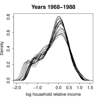
Figure 1: Kernel density estimators based on household relative income data for 1968–1988.

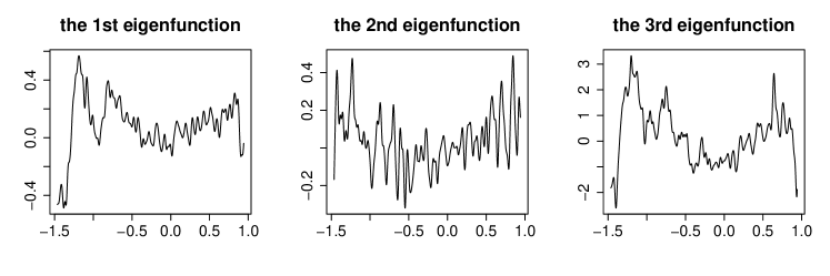
Figure 2: First three eigenfunctions obtained using data from 1968–1981.

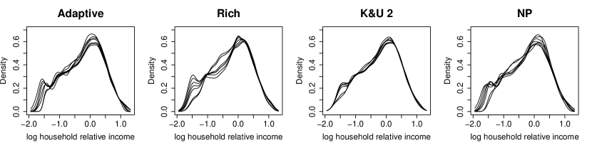
Figure 3: Estimated density functions for 1982–1988.

Table 2: Simulated IMSEs of density estimators and average MSEs of quantile estimators scaled by respective sample sizes

Method IMSE of density estimators Average MSE of quantile estimators $1982$ $1983$ $1984$ $1985$ $1986$ $1987$ $1988$ avg. $10\%$ $30\%$ $50\%$ $70\%$ $90\%$ avg. $n_{r}=500$ 1 FPC $1.00$ $1.13$ $0.75$ $0.66$ $0.61$ $0.62$ $0.54$ $0.76$ $1.21$ $0.45$ $0.26$ $0.12$ $0.20$ $0.45$ 2 FPCs $1.05$ $0.96$ $0.68$ $0.61$ $0.65$ $0.63$ $0.57$ $0.74$ $1.03$ $0.50$ $0.30$ $0.15$ $0.27$ $0.45$ Adaptive $1.05$ $0.96$ $0.68$ $0.61$ $0.65$ $0.63$ $0.57$ $0.74$ $1.03$ $0.50$ $0.30$ $0.15$ $0.27$ $0.45$ Rich $2.56$ $1.60$ $1.65$ $1.45$ $1.28$ $1.39$ $2.07$ $1.71$ $1.44$ $1.38$ $0.82$ $0.51$ $0.52$ $0.93$ K&U 1 $3.72$ $3.26$ $1.30$ $0.89$ $0.85$ $1.34$ $1.74$ $1.87$ $4.71$ $1.92$ $0.56$ $0.13$ $0.90$ $1.64$ K&U 2 $2.30$ $1.80$ $1.51$ $1.08$ $0.87$ $1.10$ $1.61$ $1.47$ $2.20$ $0.88$ $0.41$ $0.20$ $0.73$ $0.88$ NP $1.62$ $1.57$ $1.72$ $1.66$ $1.57$ $1.49$ $1.54$ $1.60$ $1.73$ $1.46$ $0.83$ $0.56$ $0.69$ $1.05$ $n_{r}=1000$ 1 FPC $1.57$ $1.96$ $1.09$ $0.98$ $1.01$ $1.05$ $0.83$ $1.21$ $1.86$ $0.62$ $0.37$ $0.16$ $0.31$ $0.66$ 2 FPCs $1.59$ $1.57$ $0.98$ $0.88$ $1.06$ $1.06$ $0.87$ $1.14$ $1.43$ $0.68$ $0.44$ $0.22$ $0.40$ $0.63$ Adaptive $1.59$ $1.57$ $0.98$ $0.88$ $1.06$ $1.06$ $0.88$ $1.15$ $1.43$ $0.69$ $0.44$ $0.22$ $0.40$ $0.64$ Rich $4.02$ $2.28$ $2.24$ $1.82$ $1.58$ $1.97$ $3.57$ $2.50$ $1.88$ $1.39$ $0.91$ $0.56$ $0.54$ $1.06$ K&U 1 $6.60$ $5.80$ $1.93$ $1.30$ $1.49$ $2.64$ $3.56$ $3.33$ $9.03$ $3.70$ $0.96$ $0.20$ $1.28$ $3.03$ K&U 2 $3.55$ $2.83$ $2.14$ $1.39$ $1.18$ $1.78$ $2.91$ $2.26$ $3.82$ $1.19$ $0.62$ $0.31$ $0.89$ $1.36$ NP $1.86$ $1.87$ $1.99$ $1.91$ $1.85$ $1.75$ $1.70$ $1.85$ $1.78$ $1.41$ $0.84$ $0.57$ $0.67$ $1.05$

Appendix

This Appendix includes proofs of the technical results and provides additional simulation results and figures. The additional experiments answer another important question: does the DRM perform well when the samples are from populations whose distributions are not connected through a few basis functions? The answer is positive, based on simulations with data sets generated from the Weibull and finite normal mixture distributions. We also include all the boxplots here to allow a more complete comparison of the various approaches. We will generally use the notation of the main paper.

Proof of Theorem 2.1

We show that the eigenvectors of $\bm{M}$ and eigenfunctions of the operator ${\mathcal{V}}$ are connected as stated in this theorem. Let

$$\bm{Q}(t)=(Q_{0}^{c}(t),\ldots,Q_{m}^{c}(t))^{\top}$$

so that we may write $\Sigma(s,t)=\bm{Q}^{\top}(s)\bm{Q}(t)$ and $\bm{M}=\int\bm{Q}(t)\bm{Q}^{\top}(t)\mathrm{d}\bar{G}(t)$. Define a matrix of eigenvectors and a diagonal matrix of eigenvalues of $\bm{M}$:

$$\bm{P}=[\bm{p}_{0},\ldots,\bm{p}_{d-1}];$$

$$\bm{\Lambda}=\mbox{diag}(\lambda_{0},\ldots,\lambda_{d-1}).$$

By the definition of eigenvalue and eigenvector, we have $\bm{M}\bm{P}=\bm{P}\bm{\Lambda}$. Next, we form a vector of possible eigenfunctions of ${\mathcal{V}}$:

$$\bm{\Psi}(t)=(\psi_{0}(t),\ldots,\psi_{d-1}(t))^{\top}=\bm{\Lambda}^{-1/2}\bm{P}^{\top}\bm{Q}(t).$$

With this preparation, we have

$${\mathcal{V}}\bm{\Psi}(t) = \int\bm{\Psi}(s)\Sigma(s,t)\mathrm{d}\bar{G}(s)$$

$$= \int\bm{\Lambda}^{-1/2}\bm{P}^{\top}\bm{Q}(s)\bm{Q}^{\top}(s)\bm{Q}(t)\mathrm{d}\bar{G}(s)$$

$$= \bm{\Lambda}^{-1/2}\bm{P}^{\top}\Big{\{}\int\bm{Q}(s)\bm{Q}^{\top}(s)\mathrm{d}\bar{G}(s)\Big{\}}\bm{Q}(t)$$

$$= \bm{\Lambda}^{-1/2}\{\bm{P}^{\top}\bm{M}\}\bm{Q}(t)$$

$$= \bm{\Lambda}^{-1/2}\bm{\Lambda}\bm{P}^{\top}\bm{Q}(t)$$

$$= \bm{\Lambda}\bm{\Psi}(t).$$

That is, ${\mathcal{V}}\bm{\Psi}(t)=\bm{\Lambda}\bm{\Psi}(t)$, which implies that $\bm{\Psi}(t)$ is indeed a vector of eigenfunctions with the eigenvalues $\lambda_{0},\ldots,\lambda_{d-1}$. This proves the first property stated in the theorem.

We next notice that

$$\int\bm{\Psi}(s)\bm{\Psi}^{\top}(s)\mathrm{d}\bar{G}(s)=\bm{\Lambda}^{-1/2}\bm{P}^{\top}\bm{M}\bm{P}\bm{\Lambda}^{-1/2}=\bm{I},$$

an identity matrix. This result confirms that the elements of $\bm{\Psi}(t)$ are orthonormal. This proves the second property stated in the theorem.

Finally, we note that the linear space spanned by $\{\bm{\Psi}_{j}(t),j=0,\ldots,d-1\}$ is a subspace of the space spanned by the elements of $\bm{\mathrm{q}}(t)$, and the ranks of both spaces are $d$. Therefore, these two spaces must be identical. This proves the third property of the theorem and completes the proof.

Proof of Theorem 4.2

This theorem states that $\hat{\bm{M}}$ is consistent for $\bm{M}$. The consistency of the eigenvalues and eigenvectors are consequences. Recall that for $0\leq i,j\leq m$,

$$\bm{M}(i,j) = \bar{E}\{\int Q^{c}_{i}(X)Q^{c}_{j}(X)\}=\int Q^{c}_{i}(x)Q^{c}_{j}(x)\mathrm{d}\bar{G}(x);$$

$$\hat{\bm{M}}({i,j}) = \int\hat{Q}^{c}_{i}(x)\hat{Q}^{c}_{j}(x)\mathrm{d}\bar{F}_{n}(x).$$

We prove this theorem by showing that for any $(i,j)$ in this range,

$$\hat{\bm{M}}(i,j)\to\bm{M}(i,j),$$

in probability, as the total sample size $N\to\infty$ under the DRM and under the model conditions specified in the theorem.

By the moment condition $\bar{E}|\log g_{i}(X)|^{3}<\infty$, it can be seen that $Q^{c}_{i}(X)$ has a finite second moment when $X$ has distribution $\bar{G}$. By the classical law of large numbers,

$$\int Q^{c}_{i}(x)Q^{c}_{j}(x)\mathrm{d}\bar{F}_{n}(x)\to\int Q^{c}_{i}(x)Q^{c}_{j}(x)\mathrm{d}\bar{G}(x)$$

almost surely. Hence, we need only show that

$$\int\{\hat{Q}^{c}_{i}(x)\hat{Q}^{c}_{j}(x)-Q^{c}_{i}(x)Q^{c}_{j}(x)\}\mathrm{d}\bar{F}_{n}(x)\to 0$$ (18)

in probability. Let us decompose this difference into

$$\hat{Q}^{c}_{i}(x)\hat{Q}^{c}_{j}(x)-Q^{c}_{i}(x)Q^{c}_{j}(x)$$ (19)

$$=\{\hat{Q}^{c}_{i}(x)-Q^{c}_{i}(x)\}\{\hat{Q}^{c}_{j}(x)-Q^{c}_{j}(x)\}$$

$$\hskip 10.00002pt+Q^{c}_{i}(x)\{\hat{Q}^{c}_{j}(x)-Q^{c}_{j}(x)\}+Q^{c}_{j}(x)\{\hat{Q}^{c}_{i}(x)-Q^{c}_{i}(x)\}.$$

By Cauchy’s inequality, we have a bound for the second term on the right-hand side of (19):

$$\Big{\{}\int{Q}^{c}_{i}(x)\{\hat{Q}^{c}_{j}(x)-Q^{c}_{j}(x)\}\mathrm{d}\bar{F}_{n}(x)\Big{\}}^{2}\leq\int\{{Q}^{c}_{i}(x)\}^{2}\mathrm{d}\bar{F}_{n}(x)\int\{\hat{Q}^{c}_{j}(x)-Q^{c}_{j}(x)\}^{2}\mathrm{d}\bar{F}_{n}(x).$$

Under the moment condition, the first multiplication factor in the above expression has a finite limit by the law of large numbers. Thus, if

$$\int\{\hat{Q}^{c}_{j}(x)-Q^{c}_{j}(x)\}^{2}\mathrm{d}\bar{F}_{n}(x)\to 0$$ (20)

in probability, then

$$\int{Q}^{c}_{i}(x)\{\hat{Q}^{c}_{j}(x)-Q^{c}_{j}(x)\}\mathrm{d}\bar{F}_{n}(x)\to 0.$$

We can use similar bounds from Cauchy’s inequality for the other terms in (19) to arrive at the same conclusion. These lead to (18). Hence, our task is reduced to proving (20).

We first show that for each $i$,

$$\int\{\log\hat{g}_{i}(x)-\log g_{i}(x)\}^{2}\mathrm{d}\bar{F}_{n}(x)\to 0.$$ (21)

Let ${\mathcal{X}}_{\delta,i}=\{x:g_{i}(x)\leq\delta\}$ with $\delta=N^{-1/3}$ to simplify the notation. We can see that

$$\int_{{\mathcal{X}}_{\delta,i}}|\log g_{i}(x)|^{2}\mathrm{d}\bar{F}_{n}(x) \leq\int_{{\mathcal{X}}_{\delta,i}}\frac{3|\log g_{i}(x)|^{3}}{\log N}\mathrm{d}\bar{F}_{n}(x)$$

$$\leq 3\log^{-1}N\int|\log g_{i}(x)|^{3}\mathrm{d}\bar{F}_{n}(x)\to 0,$$

since the second factor is $O_{p}(1)$ under the moment condition $\bar{E}|\log g_{i}(X)|^{3}<\infty$.

Since $\hat{g}_{i}(x)$ is uniformly consistent for $g_{i}(x)$, without loss of generality, we assume $\hat{g}_{i}(x)<1$ to simplify the presentation. Recall that $\hat{g}_{i}(x)\geq C_{i}(\log N/N)^{2/5}$ by design, so we get

$$|\log\hat{g}_{i}(x)|^{2}\leq\log^{2}N,$$

when $N$ is large enough. We have removed some harmless constants to simplify the expression. Note that by a well-known result about the empirical distribution, we have $\sup_{x}|\bar{F}_{n}(x)-\bar{G}(x)|=O((\log N/N)^{1/2})$. Hence,

$$\int_{{\mathcal{X}}_{\delta,i}}|\log\hat{g}_{i}(x)|^{2}\mathrm{d}\bar{F}_{n}(x)\leq(\log^{2}N)\bar{F}_{n}\{{\mathcal{X}}_{\delta,i}\}=O_{p}((\log N)^{-1})=o_{p}(1).$$

Combining two order assessments of the integration of $\log g_{i}(x)$ and $\log\hat{g}_{i}(x)$ on ${{\mathcal{X}}_{\delta,i}}$, we arrive at a partial conclusion of (21):

$$\int_{{\mathcal{X}}_{\delta,i}}\{\log\hat{g}_{i}(x)-\log g_{i}(x)\}^{2}\mathrm{d}\bar{F}_{n}(x)\to 0$$

in probability. We now use Lemma 4.1. Let ${{\mathcal{X}}}^{c}_{\delta,i}$ be the complement of ${\mathcal{X}}_{\delta,i}$. With $\delta=N^{-1/3}$ and $\sup_{x}|\hat{g}_{i}(x)-g_{i}(x)|=O((\log N/N)^{2/5})$, we have

$$\inf_{x\in{{\mathcal{X}}}^{c}_{\delta,i}}\hat{g}_{i}(x)=N^{-1/3}(1+o(1)).$$

For simplicity, we proceed as if $\inf_{x\in{{\mathcal{X}}}^{c}_{\delta,i}}\hat{g}_{i}(x)=N^{-1/3}$ so that

$$\sup_{x\in{{\mathcal{X}}}^{c}_{\delta,i}}|\log\hat{g}_{i}(x)-\log g_{i}(x)|^{2}\leq N^{2/3}\sup_{x\in{{\mathcal{X}}}^{c}_{\delta,i}}|\hat{g}_{i}(x)-g_{i}(x)|^{2}=o(1).$$

This implies

$$\int_{{\mathcal{X}}^{c}_{\delta,i}}|\log\hat{g}_{i}(x)-\log g_{i}(x)|^{2}\mathrm{d}\bar{F}_{n}(x)=o(1).$$

This completes the proof of (21).

Note that $\hat{Q}_{i}^{c}(x)-Q_{i}^{c}(x)$ is composed of various linear combinations of $\log\hat{g}_{i}(x)-\log g_{i}(x)$. We can easily see that (21) implies (20). We omit these tedious details here because they are conceptually simple.

Proof of Theorem 4.3

This theorem states that the eigenvalues and eigenvectors of $\hat{\bm{M}}$ are consistent for those of $\bm{M}$. Because the eigenvalues and eigenvectors are continuous functions of $\bm{M}$, and $\hat{\bm{M}}$ is consistent for $\bm{M}$ as proved in the previous section, the conclusions are obvious when all the eigenvalues are different. When some nonzero eigenvalues are equal, their eigenvectors form a linear space that is continuous with respect to $\bm{M}$. The consistency of subspaces suffices.

We have shown in the previous section, as a side fact, that $\hat{Q}^{c}_{r}(x)$ is consistent for $Q^{c}_{r}(x)$. Therefore, the consistency of $\hat{\psi}_{j}(x)$ is obvious by inspecting its definition. Interested readers are referred to a useful lemma in Kneip and Utikal (2001, Lemma A.1) for details regarding the relationship between the eigensystem of a matrix $A$ and the eigensystem of a perturbed matrix $A+B$.

Additional figures

We include here some additional figures for the simulation studies and real-data analysis in the main text.

Figure 4 presents the six density functions of Scenario 4, which satisfy the DRM with tailor-designed log density ratios. These distributions have similar shapes, but the commonly used basis functions under DRM do not work. This example highlights the need for adaptive basis functions.

Figures 5–8 present boxplots of two performance measures: the integrated squared errors (ISE) of the density estimators and the simulated squared errors (SE) of the quantile estimators. That is, these values are not averaged over $N_{\mathrm{rep}}=1000$ repetitions. The boxplots shed light on the sample distributions of these estimators, rather than merely their biases and variances. We include the estimators for the samples from the four scenarios presented in the main text. Figure 9 shows the boxplots of these two measures in the real-data example. The sample size is $1000$, and we have removed extreme values for clearer illustrations.

Our method is not always the best, but its performance is often close to that of the DRM with the “true” basis function. It outperforms the nonparametric methods in almost every case, and it usually outperforms the method of Kneip and Utikal (2001).

Figure 4: Density functions for the six self-designed distributions.

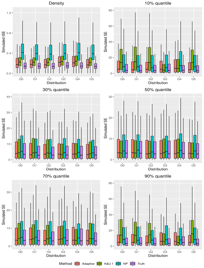
Figure 5: Boxplots of simulated ISEs of density estimators and simulated SEs of quantile estimators. Data generated from normal distributions with equal variances (Scenario 1).

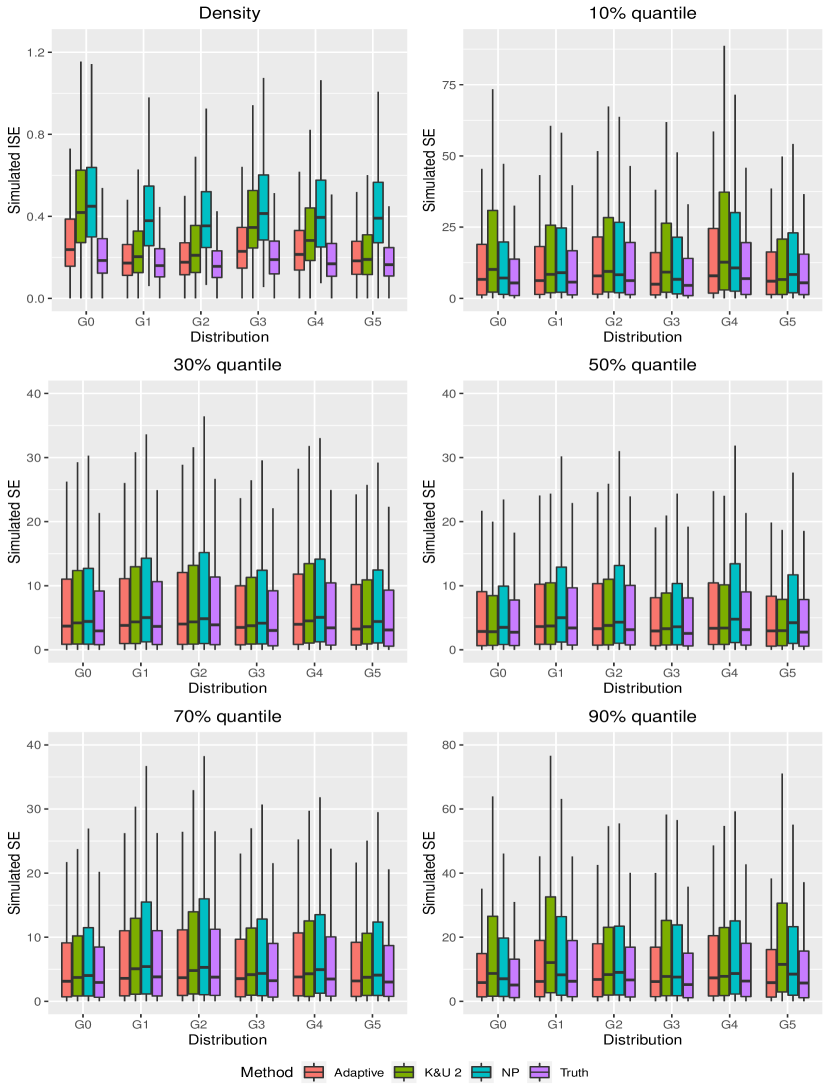
Figure 6: Boxplots of simulated ISEs of density estimators and simulated SEs of quantile estimators. Data generated from normal distributions with unequal variances (Scenario 2).

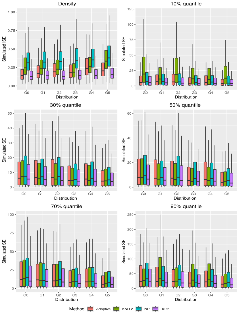
Figure 7: Boxplots of simulated ISEs of density estimators and simulated SEs of quantile estimators. Data generated from gamma distributions (Scenario 3).

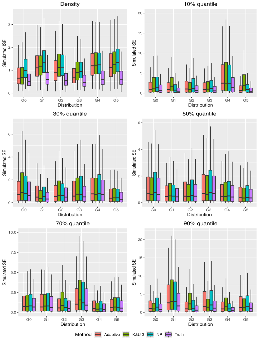
Figure 8: Boxplots of simulated ISEs of density estimators and simulated SEs of quantile estimators. Data generated from self-designed distributions (Scenario 4).

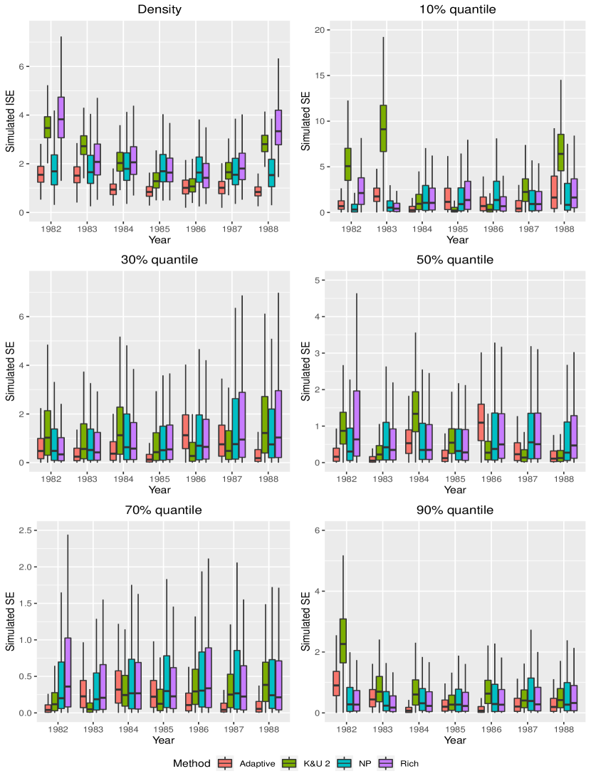
Figure 9: Boxplots of simulated ISEs of density estimators and simulated SEs of quantile estimators. Data from the real-data example.

Simulations based on multiple samples from distributions that do not satisfy DRM

While data from multiple populations of a similar nature should share some latent structure, there is no guarantee that there is always a helpful DRM with a meaningful basis function $\bm{\mathrm{q}}(x)$. Some studies suggest that a DRM coupled with a rich basis function such as $\bm{\mathrm{q}}(x)=(|x|^{1/2},x,x^{2},\log(1+|x|))^{\top}$ will work well. It is likely that a rich basis function will often but not always permit a good fit of the DRM to the data. In this section, we present simulation results based on data generated from Weibull distributions and finite mixture distributions. There is no apparent DRM with a sensible choice of basis function that includes these distributions. One may saturate the density ratio space to ensure validity, but such a DRM does not truly help in terms of connecting these populations.

We fit the data with the DRM using the proposed adaptive basis function with varying numbers of eigenfunctions. We also implement the method of Kneip and Utikal (2001) and fit a DRM coupled with a rich basis function. We wish to discover which approach will lead to consistent efficiency gains in the density and quantile estimation.

We first consider $m+1=6$ samples generated from six Weibull distributions. The probability density function of a Weibull random variable is

$$f(x;\lambda,k)=\frac{k}{\lambda}(x/\lambda)^{k-1}\exp\{-(x/\lambda)^{k}\},\hskip 14.22636ptx\geq 0,$$

where $k,\lambda$ are positive values known as the shape and scale parameters. We set the shape parameters to $(4.5,5,6,6.5,7,7.5)$ and the scale parameters to $(10,9,11,11.5,12.5,12)$.

We next consider $m+1=6$ samples from six two-component normal mixture distributions. These distributions are as follows:

$$G_{j}=\lambda_{j}N(\mu_{1,j},\sigma_{1,j}^{2})+(1-\lambda_{j})N(\mu_{2,j},\sigma_{2,j}^{2}),\hskip 14.22636ptj=0,1,\ldots,5.$$

We choose the six mixture distributions as follows. We set the mixing proportions to $(\lambda_{0},\ldots,\lambda_{5})=(0.5,0.5,0.3,0.5,0.4,0.2)$; the component means to $(\mu_{1,0},\ldots,\mu_{1,5})=(15,15,15.5,16,14.5,15)$ and $(\mu_{2,0},\ldots,\mu_{2,5})=(18,18,17,19,17,16)$; and the component variances to $(\sigma_{1,0}^{2},\ldots,\sigma_{1,5}^{2})=(3,3,3.5,3,3.5,3)$ and $(\sigma_{2,0}^{2},\ldots,\sigma_{2,5}^{2})=(3,3.5,4,4,4.5,3)$.

In both scenarios, we generate $1000$ sets of independent and multiple samples of sizes $n_{r}=500,1000$. Table 3 gives the IMSEs of the density estimators and the average MSEs of the quantile estimators across the five quantile levels 10%, 30%, 50%, 70%, and 90%. The abbreviations used in this table are the same as those in the main text. Based on the simulation results, we find that the DRM-based estimators have a worthwhile gain in efficiency compared to purely nonparametric data analysis. The use of a single eigenfunction should be avoided. The fully adaptive basis functions work well in most cases, and the rich basis function seems to have the best performance. If one uses sufficient orthonormal functions in the method of Kneip and Utikal (2001), the resulting estimates are in line with the nonparametric estimates.

In summary, for these two examples, applying the DRM with either a fully adaptive basis function or the rich basis function can lead to efficiency gains. In applications, one cannot know if the rich basis will work well, and therefore we recommend the fully adaptive DRM approach.

Table 3: Simulated IMSEs of density estimators and average MSEs of quantile estimators scaled by respective sample sizes.

Method IMSE of density estimators Average MSE of quantile estimators $G_{0}$ $G_{1}$ $G_{2}$ $G_{3}$ $G_{4}$ $G_{5}$ avg. $10\%$ $30\%$ $50\%$ $70\%$ $90\%$ avg. $n_{r}=500$, Weibull 1 FPC $0.67$ $1.23$ $0.31$ $0.31$ $0.56$ $0.73$ $0.64$ $31.58$ $11.77$ $5.91$ $7.19$ $21.89$ $15.67$ 2 FPCs $0.32$ $0.51$ $0.28$ $0.29$ $0.34$ $0.35$ $0.35$ $12.52$ $7.14$ $5.45$ $4.87$ $6.33$ $7.26$ Adaptive $0.43$ $0.70$ $0.30$ $0.29$ $0.43$ $0.45$ $0.43$ $18.11$ $8.49$ $5.51$ $5.36$ $10.40$ $9.57$ Rich $0.33$ $0.35$ $0.27$ $0.28$ $0.33$ $0.34$ $0.32$ $11.82$ $6.52$ $5.08$ $4.77$ $5.70$ $6.78$ K&U 1 $0.21$ $0.69$ $2.29$ $1.27$ $2.21$ $0.77$ $1.24$ $49.69$ $13.32$ $11.72$ $23.57$ $52.68$ $30.20$ K&U 2 $0.29$ $0.41$ $0.44$ $0.30$ $0.45$ $0.66$ $0.43$ $17.76$ $7.14$ $5.01$ $5.08$ $10.64$ $9.12$ NP $0.42$ $0.49$ $0.46$ $0.51$ $0.51$ $0.55$ $0.49$ $15.15$ $8.08$ $6.21$ $5.84$ $7.69$ $8.59$ $n_{r}=1000$, Weibull 1 FPC $1.29$ $1.90$ $0.41$ $0.40$ $0.87$ $1.24$ $1.02$ $56.84$ $18.51$ $6.53$ $8.35$ $36.29$ $25.30$ 2 FPCs $0.37$ $0.60$ $0.32$ $0.32$ $0.40$ $0.44$ $0.41$ $12.91$ $7.48$ $5.58$ $4.86$ $6.55$ $7.47$ Adaptive $0.37$ $0.59$ $0.32$ $0.32$ $0.40$ $0.44$ $0.41$ $12.91$ $7.29$ $5.48$ $4.86$ $6.57$ $7.42$ Rich $0.40$ $0.40$ $0.30$ $0.31$ $0.35$ $0.42$ $0.36$ $12.08$ $6.39$ $5.11$ $4.89$ $5.63$ $6.82$ K&U 1 $0.26$ $1.19$ $4.31$ $2.29$ $4.41$ $1.24$ $2.28$ $88.26$ $20.10$ $19.14$ $43.17$ $96.79$ $53.49$ K&U 2 $0.36$ $0.51$ $0.62$ $0.34$ $0.54$ $1.04$ $0.57$ $22.56$ $7.70$ $5.34$ $5.35$ $11.99$ $10.59$ NP $0.48$ $0.57$ $0.57$ $0.61$ $0.59$ $0.67$ $0.58$ $15.05$ $7.94$ $6.13$ $5.97$ $7.62$ $8.54$ $n_{r}=500$, normal mixture 1 FPC $0.28$ $0.36$ $0.74$ $0.78$ $1.09$ $0.76$ $0.67$ $62.96$ $31.63$ $16.68$ $10.82$ $14.20$ $27.26$ 2 FPCs $0.27$ $0.23$ $0.31$ $0.39$ $0.26$ $0.36$ $0.30$ $9.76$ $7.47$ $7.22$ $7.74$ $11.84$ $8.81$ 3 FPCs $0.33$ $0.30$ $0.40$ $0.36$ $0.31$ $0.41$ $0.35$ $9.94$ $7.62$ $8.00$ $8.49$ $11.92$ $9.20$ 4 FPCs $0.39$ $0.37$ $0.42$ $0.36$ $0.35$ $0.44$ $0.39$ $10.38$ $7.78$ $8.27$ $8.78$ $12.29$ $9.50$ Adaptive $0.27$ $0.23$ $0.32$ $0.39$ $0.27$ $0.36$ $0.31$ $9.95$ $7.59$ $7.33$ $7.77$ $11.84$ $8.90$ Rich $0.27$ $0.25$ $0.32$ $0.29$ $0.26$ $0.31$ $0.28$ $9.07$ $7.01$ $6.96$ $7.72$ $11.11$ $8.37$ K&U 1 $0.30$ $0.24$ $1.10$ $0.62$ $0.64$ $1.22$ $0.69$ $48.23$ $20.27$ $10.25$ $8.60$ $27.80$ $23.03$ K&U 2 $0.34$ $0.27$ $0.61$ $0.43$ $0.38$ $0.63$ $0.44$ $17.03$ $8.79$ $7.85$ $8.79$ $21.22$ $12.74$ K&U 3 $0.33$ $0.32$ $0.46$ $0.40$ $0.37$ $0.52$ $0.40$ $14.79$ $7.76$ $7.26$ $8.47$ $16.17$ $10.89$ K&U 4 $0.37$ $0.37$ $0.45$ $0.39$ $0.39$ $0.52$ $0.41$ $14.33$ $7.58$ $7.21$ $8.44$ $15.40$ $10.59$ NP $0.39$ $0.40$ $0.46$ $0.39$ $0.39$ $0.53$ $0.43$ $12.15$ $8.48$ $8.67$ $9.53$ $14.08$ $10.58$ $n_{r}=1000$, normal mixture 1 FPC $0.45$ $0.59$ $1.31$ $1.28$ $2.07$ $1.20$ $1.15$ $119.08$ $56.71$ $25.46$ $12.27$ $15.54$ $45.81$ 2 FPCs $0.38$ $0.27$ $0.38$ $0.54$ $0.30$ $0.42$ $0.38$ $9.99$ $8.14$ $8.09$ $8.36$ $12.12$ $9.34$ 3 FPCs $0.40$ $0.32$ $0.42$ $0.42$ $0.34$ $0.46$ $0.39$ $10.06$ $7.76$ $8.19$ $8.68$ $11.69$ $9.28$ 4 FPCs $0.41$ $0.40$ $0.43$ $0.39$ $0.37$ $0.50$ $0.42$ $10.20$ $7.79$ $8.22$ $8.76$ $11.80$ $9.36$ Adaptive $0.38$ $0.27$ $0.38$ $0.54$ $0.30$ $0.42$ $0.38$ $9.97$ $8.12$ $8.08$ $8.35$ $12.10$ $9.33$ Rich $0.36$ $0.29$ $0.39$ $0.34$ $0.29$ $0.35$ $0.34$ $9.51$ $7.40$ $7.06$ $8.09$ $10.96$ $8.60$ K&U 1 $0.51$ $0.40$ $2.00$ $0.97$ $1.28$ $2.06$ $1.20$ $86.96$ $35.82$ $14.78$ $9.26$ $40.05$ $37.37$ K&U 2 $0.48$ $0.32$ $1.01$ $0.57$ $0.48$ $0.84$ $0.62$ $18.94$ $10.26$ $9.38$ $9.57$ $29.15$ $15.46$ K&U 3 $0.38$ $0.37$ $0.55$ $0.46$ $0.44$ $0.65$ $0.48$ $16.31$ $8.16$ $7.57$ $8.80$ $16.85$ $11.54$ K&U 4 $0.43$ $0.43$ $0.53$ $0.46$ $0.46$ $0.65$ $0.49$ $15.61$ $7.96$ $7.47$ $8.76$ $16.17$ $11.19$ NP $0.47$ $0.48$ $0.53$ $0.46$ $0.46$ $0.66$ $0.51$ $12.37$ $8.65$ $8.77$ $9.57$ $13.94$ $10.66$

References

• Akaike (1973) H. Akaike. Information theory and an extension of the maximum likelihood principle. In B. N. Petrov and F. Csáki, editors, Second International Symposium on Information Theory, pages 267–281. Budapest: Académiai Kiadó, 1973.
• Anderson (1979) J. Anderson. Multivariate logistic compounds. Biometrika, 66(1):17–26, 1979.
• Arveson (2006) W. Arveson. A Short Course on Spectral Theory, volume 209. Springer Science & Business Media, 2006.
• Cai et al. (2017) S. Cai, J. Chen, and J. V. Zidek. Hypothesis testing in the presence of multiple samples under density ratio models. Statistica Sinica, 27:761–783, 2017.
• Chen and Liu (2013) J. Chen and Y. Liu. Quantile and quantile-function estimations under density ratio model. The Annals of Statistics, 41(3):1669–1692, 2013.
• Chen et al. (2016) J. Chen, P. Li, Y. Liu, and J. V. Zidek. Monitoring test under nonparametric random effects model. arXiv:1610.05809, 2016.
• Conway (2007) J. B. Conway. A Course in Functional Analysis, volume 96 of Graduate Texts in Mathematics. Springer New York, 2007.
• De Oliveira and Kedem (2017) V. De Oliveira and B. Kedem. Bayesian analysis of a density ratio model. The Canadian Journal of Statistics, 45(3):274–289, 2017.
• Fokianos (2007) K. Fokianos. Density ratio model selection. Journal of Statistical Computation and Simulation, 77(9):805–819, 2007.
• Fokianos and Kaimi (2006) K. Fokianos and I. Kaimi. On the effect of misspecifying the density ratio model. Annals of the Institute of Statistical Mathematics, 58(3):475–497, 2006.
• Fokianos et al. (2001) K. Fokianos, B. Kedem, J. Qin, and D. A. Short. A semiparametric approach to the one-way layout. Technometrics, 43(1):56–65, 2001.
• Huang and Rathouz (2012) A. Huang and P. J. Rathouz. Proportional likelihood ratio models for mean regression. Biometrika, 99(1):223–229, 2012.
• Kedem et al. (2008) B. Kedem, G. Lu, R. Wei, and P. D. Williams. Forecasting mortality rates via density ratio modeling. The Canadian Journal of Statistics, 36(2):193–206, 2008.
• Kneip and Utikal (2001) A. Kneip and K. J. Utikal. Inference for density families using functional principal component analysis. Journal of the American Statistical Association, 96(454):519–542, 2001.
• Li et al. (2017) P. Li, Y. Liu, and J. Qin. Semiparametric inference in a genetic mixture model. Journal of the American Statistical Association, 112(519):1250–1260, 2017.
• Luo and Tsai (2012) X. Luo and W. Y. Tsai. A proportional likelihood ratio model. Biometrika, 99(1):211–222, 2012.
• Office for National Statistics (1961–2001) Office for National Statistics. Family expenditure survey, 1961–2001, 1961–2001. UK Data Archive. GB 1956 FES, https://archiveshub.jisc.ac.uk/data/gb1956-fes.
• Owen (2001) A. B. Owen. Empirical Likelihood. Chapman & Hall/CRC, New York, 2001.
• Parzen (1962) E. Parzen. On estimation of a probability density function and mode. The Annals of Mathematical Statistics, 33(3):1065–1076, 1962.
• Prakasa Rao (1983) B. Prakasa Rao. Nonparametric Functional Estimation. Academic Press, New York, 1983.
• Qin (1993) J. Qin. Empirical likelihood in biased sample problems. The Annals of Statistics, 21(3):1182–1196, 1993.
• Qin (1998) J. Qin. Inferences for case-control and semiparametric two-sample density ratio models. Biometrika, 85(3):619–630, 1998.
• Qin (2017) J. Qin. Biased Sampling, Over-identified Parameter Problems and Beyond. Springer, 2017.
• Qin and Zhang (1997) J. Qin and B. Zhang. A goodness-of-fit test for logistic regression models based on case-control data. Biometrika, 84(3):609–618, 1997.
• Ramsay and Silverman (2005) J. Ramsay and B. Silverman. Functional Data Analysis. Springer Science & Business Media, 2005.
• Rathouz and Gao (2009) P. J. Rathouz and L. Gao. Generalized linear models with unspecified reference distribution. Biostatistics, 10(2):205–218, 2009.
• Rice and Silverman (1991) J. A. Rice and B. W. Silverman. Estimating the mean and covariance structure nonparametrically when the data are curves. Journal of the Royal Statistical Society: Series B (Methodological), 53(1):233–243, 1991.
• Rosenblatt (1956) M. Rosenblatt. Remarks on some nonparametric estimates of a density function. The Annals of Mathematical Statistics, 27(3):832–837, 1956.
• Schwarz (1978) G. Schwarz. Estimating the dimension of a model. The Annals of Statistics, 6(2):461–464, 1978.
• Silverman (1978) B. W. Silverman. Weak and strong uniform consistency of the kernel estimate of a density and its derivatives. The Annals of Statistics, pages 177–184, 1978.
• Silverman (1986) B. W. Silverman. Density Estimation for Statistics and Data Analysis, volume 26. CRC Press, 1986.
• Sugiyama et al. (2012) M. Sugiyama, T. Suzuki, and T. Kanamori. Density Ratio Estimation in Machine Learning. Cambridge University Press, 2012.
• Tan (2009) Z. Tan. A note on profile likelihood for exponential tilt mixture models. Biometrika, 96(1):229–236, 2009.
• Vardi (1982) Y. Vardi. Nonparametric estimation in the presence of length bias. The Annals of Statistics, 10(2):616–620, 1982.
• Vardi (1985) Y. Vardi. Empirical distributions in selection bias models. The Annals of Statistics, 13(1):178–203, 1985.
• Wang et al. (2016) J.-L. Wang, J.-M. Chiou, and H.-G. Müller. Functional data analysis. Annual Review of Statistics and Its Application, 3:257–295, 2016.
• Wied and Weißbach (2012) D. Wied and R. Weißbach. Consistency of the kernel density estimator: A survey. Statistical Papers, 53(1):1–21, 2012.
• Zhuang et al. (2019) W. Zhuang, B. Hu, and J. Chen. Semiparametric inference for the dominance index under the density ratio model. Biometrika, 106(1):229–241, 2019.