Target Localization using Bistatic and Multistatic Radar with 5G NR Waveform
Abstract
Joint communication and sensing allows the utilization of common spectral resources for communication and localization, reducing the cost of deployment. By using fifth generation (5G) New Radio (NR) (i.e., the 3rd Generation Partnership Project Radio Access Network for 5G) reference signals, conventionally used for communication, this paper shows sub-meter precision localization is possible at millimeter wave frequencies. We derive the geometric dilution of precision of a bistatic radar configuration, a theoretical metric that characterizes how the target location estimation error varies as a function of the bistatic geometry and measurement errors. We develop a 5G NR compliant software test bench to characterize the measurement errors when estimating the time difference of arrival and angle of arrival with 5G NR waveforms. The test bench is further utilized to demonstrate the accuracy of target localization and velocity estimation in several indoor and outdoor bistatic and multistatic configurations and to show that on average, the bistatic configuration can achieve a location accuracy of 10.0 cm over a bistatic range of 25 m, which can be further improved by deploying a multistatic radar configuration.
Index Terms:
5G NR; Bistatic Radar; Multistatic Radar; geometric dilution of precision (GDOP); 3GPP; localization; positioning; position locationI Introduction
As communication systems move towards higher frequency bands, significantly wider system bandwidths become available. The frequency range 2 (FR2) defined in the 3rd Generation Partnership Project (3GPP) fifth generation (5G) New Radio (NR) encompasses millimeter wave (mmWave) frequencies from 24.25 to 52.6 GHz and allows a maximum system bandwidth of 400 MHz. As the wireless industry moves towards frequencies above 90 GHz (and eventually Terahertz frequencies) in the future, spectrum spanning several Gigahertz will become available [1, 2]. While mobile communication systems evolved with emergency 911 (E-911) capabilities bolted on to the infrastructure to provide position location to within 100 m as part of early second and third generation cellular systems [3], future wireless systems will exploit massive bandwidths to provide simultaneous communications and sensing capabilities. Centimeter level localization [4] is one such application that can be made possible by joint communication and sensing (JCS) without the need of additional sensing hardware, thus reducing cost, control overhead, and power consumption that used to be required to build a separate localization system [5, 6, 3].
For user equipment (UE) positioning, the current 3GPP standards uses measurement techniques, such as observed time-difference of arrival (OTDOA) and uplink time difference of arrival (UTDOA), where the UE to be localized must transmit or receive a reference signal [4]. In OTDOA positioning, the UE receives known reference signals (the positioning reference signal (PRS)) from multiple base stations (BSs) and the propagation time differences of the reference signal are measured. In UTDOA positioning, the UE transmits reference signals (the sounding reference signal (SRS)) and the propagation time differences are measured at multiple BSs [4]. In addition to UE positioning, OTDOA and UTDOA measurements may enable JCS applications such as device-free target localization, wherein the target to be localized is not required to transmit or receive signals. In assisted living facilities, device-free localization could be used for fall detection [7]. In vehicle-to-everything (V2X) applications, device-free localization is required for pedestrian avoidance. Security applications such as intrusion detection in homes and offices are made possible via device-free localization without the knowledge or cooperation of the intruder [8].
Radars have long been used for target detection and localization. With JCS, radar functionality can be incorporated into BS and UE [6]. In monostatic radar configurations, a single node (e.g., a UE or a BS in the network) is used for both transmission and reception. The architecture of a monostatic radar may be half-duplex, wherein the node must transmit and receive over two non-overlapping time intervals, or full-duplex, wherein the node may simultaneously transmit and receive. Half-duplex monostatic radars may suffer from the drawback that the radar may not be able to sense nearby targets. The minimum radar sensing distance, which is the minimum distance the target (to be localized) must be from the radar transmitter, may be very large. Half-duplex monostatic radars cannot detect target reflections until the transmitted pulse completely leaves the transmitter (TX) antenna and the radar switches from TX to receiver (RX) mode, during which targets closer than the minimum radar sensing distance cannot be detected. For example, for a 5G NR system at mmWave with 120 kHz subcarrier spacing, assuming that the minimum pulse duration is at least an OFDM symbol duration, i.e., 8.33 us, the minimum radar sensing distance would be 1.25 km due to the speed of radiowave propagation.
Full-duplex monostatic radars can eliminate the long minimum ranging distance problem; however, the challenge of self-interference must then be addressed. Self-interference may be canceled through active RF cancellation methods, while preserving the reflected target echo [9]. The suitability of LTE reference signals for target localization was analyzed in [10], by using the ambiguity function, which is the output of the matched filter at the RX when the known radar waveform is used as the filter input. The LTE reference signals were found to be suitable for full duplex monostatic radar applications, with a range resolution of 7.56 m using a bandwidth of 20 MHz [10].
Bistatic and multistatic radar configurations, the focus of the rest of the paper, require two or more nodes to operate, wherein full duplex communication is not required because the TX and RX are not collocated. Therefore, bistatic and multistatic configurations are easier to implement with current communication hardware than monostatic configuration. Besides nodes of mobile wireless communication systems (e.g., BS, UE) implicitly form bistatic or multistatic configurations with potential targets, hence network nodes may be used for target localization as well as for communications [6].
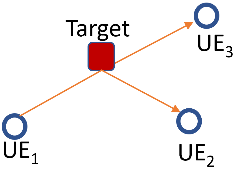
In this work, we analyze the localization accuracy of bistatic and multistatic radar using the 5G NR demodulation reference signal (DMRS). We provide an overview of bistatic and multistatic target localization techniques, where an analytical framework is also presented to calculate the GDOP, a metric to characterize the target location estimation error as a function of the bistatic geometry and the measurement errors. Prior works in [11, 12] calculated the GDOP with Angle of Arrival (AOA) and time of arrival (TOA) measurements with bistatic and multistatic radar. In this work we extend such analysis to calculate the GDOP with AOA and Time-Difference of Arrival (TDOA) measurements with a bistatic radar. We further develop a 5G NR compliant software test bench, consisting of an easy to use software simulation platform in MATLAB, to derive the TDOA and AOA measurements errors using 5G NR DMRS for measurements under different bistatic scenarios, i.e. varying the TX-target-RX separation and target radar cross-section (RCS) in ideal channel conditions. The AOA and TDOA measurement errors are then used to derive the target location estimation errors for different bistatic as well as multistatic scenarios. We show that for a given target, the GDOP can be used as a metric by which to select the best nodes for localization, as well as the mode of operation of each node (transmit or receive). For instance, as seen in Fig. 1, for the given target, bistatic measurements using nodes UE1 and UE2 may be preferred over the measurements using nodes UE1 and UE3 for target localization due to lower GDOP. We explicitly derive the GDOP in Section II-B.
The rest of the paper is organized as follows: Section II provides an overview of bistatic and multistatic target localization techniques along with the details of GDOP. The details of 5G NR compliant test bench used to derive the AOA and TDOA measurement errors are given in Section III. Section IV provides simulation results of target location estimation errors for various bistatic and multistatic scenarios. Section V concludes the paper.
II Localization in Bi/Multi-static Radar Configuration
II-A Bistatic Localization Geometry
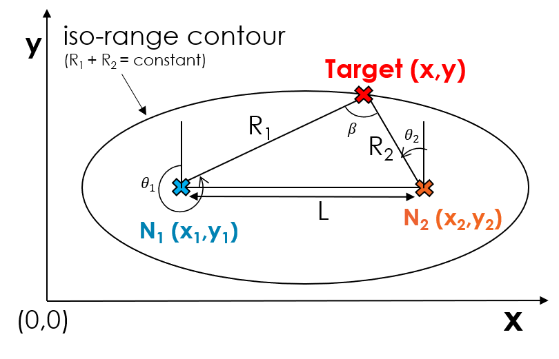
The bistatic radar configurations employs two nodes, and , at different known locations , and , respectively. A known signal, called a reference signal, may be transmitted from either node. The unknown position of the target is determined by measuring the TDOA and AOA of the reference signal at the RX node. The bistatic radar has two modes of operation — in mode 1, transmits the reference signal to and in mode 2, transmits the reference signal to . We now discuss how the position of the target is determined in mode 1, and it will be clear that a symmetric procedure is applicable to mode 2.
In mode 1, the bistatic RX () measures the time delay between the direct signal from the TX () and the signal reflected off the target, i.e., the TDOA :
| (1) |
where is the distance of the target from , is the distance of the target from , L is the distance between and , and is the speed of light. Target locations where is constant lie on an ellipse (with focii at and ) called the iso-range contour, as shown in Fig 2. also measures the AOA () of the reflected signal. Using the TDOA and AOA, can be calculated as follows [13]:
| (2) |
Finally, the position of the target () is estimated to be ).
The TDOA and AOA estimation performance of a bistatic radar depends on the signal-to-noise ratio (SNR) at the RX, given by [14]:
| (3) |
where is the TX power in watts, and are the TX and RX antenna gains, is the wavelength of the transmitted signal, is the bistatic RCS of the target, k is the Boltzmann constant ( J/K), is the RX noise temperature, and is the noise bandwidth at the RX. Note that constant SNR curves (called Cassini curves) do not coincide with iso-range contour, i.e., the SNR received at the RX varies for different target locations on an iso-range [14].
II-B Bistatic target localization GDOP with TDOA and AOA measurements
The GDOP expresses the sensitivity of the target location estimate to measurement errors, (e.g., errors in TDOA, AOA) as well as errors in the known location of and . High GDOP indicates that the radar geometry is very sensitive to error in measurements – a slight error in measurements leads to large position location error. A low GDOP is preferred, where the position location error is insensitive to measurement errors.
GDOP has been calculated for various radar localization methods, such as systems where only TOA is measured or for hybrid TOA/AOA localization methods [11]. Although the GDOP of joint AOA and TDOA has been calculated using two transmitting reference nodes [15], to the best of our knowledge, the GDOP of a bistatic radar measuring AOA and TDOA for device-free passive localization has not been examined, as shall now be derived.
The measured TDOA and AOA can be expressed in terms of the coordinates of the target, , and as follows [11]:
| (4) | ||||
| (5) |
where for the AOA measurement at node and , respectively.
Taking the total derivative of the measurements, , , and with respect to the coordinates of the target, , and we find:
| (6) | |||
| (7) | |||
| (8) |
| (9) | |||
| (10) | |||
| (11) |
Let , where
| (12) | |||
| (13) | |||
| (14) |
For small errors, the differentials of the target position , TDOA (), AOA ( and ), node positions and are approximately equal to the estimation errors [11]. Let , and denote the estimation errors of target position, and node position in vector form, respectively. We now evaluate the relation between and the geometry of the nodes.
In mode 1, since is measured at , let denote the measurements in vector form. Taking the total derivative of the measurement vector, we obtain:
| (15) |
where
| (16) | ||||
| (17) |
Thus,
| (18) | ||||
| (19) |
where is the error covariance matrix, , = diag(, ) assuming the TDOA and AOA measurement errors are uncorrelated, and = diag(, , , ) assuming the errors in the node positions are uncorrelated. and are the variances in measured TDOA and AOA respectively, while , , , and are the variances in the coordinates of and . Note that , the target position estimation error, is a function of the position of the target on the iso-range contour with different points on the contour having different target location error even though the TDOA and AOA errors are the same. Finally,
| (20) |
The GDOP can be similarly derived for mode 2 by by replacing with in the definitions of , and .
II-C Extension to Multistatic Configurations
In scenarios when there are more than two nodes capable of performing TDOA and AOA measurements from other reference nodes, the position of the target may be obtained by estimating the target position for different node pairs and then combining the estimates in an intelligent manner. Measurements at the nodes may be treated as soft information [16]. The measurements from each node pair may be sent to a central server (or to one of the nodes involved in the measurements), where a single position estimate is obtained using soft information from all the nodes. One method to determine the target position is to minimize , the weighted least squares loss metric defined as [17]:
| (21) |
where there are node pairs conducting measurements, and are weighting parameters assigned to TDOA and AOA measurements, respectively ( has units while is unit-less), and are the measured TDOA and AOA at the node pair, respectively, while and are defined as in (4) and (5), respectively, and are the weights assigned to each node pair, inversely proportionate to the predicted positioning error of the node pair (). Weighted averaging with ensures that node pairs with poor geometry (high ) will have a lower impact on the position estimate. The optimization problem may be solved by techniques such as the Levenberg–Marquardt algorithm [18].
III Bi/Multi-static Configuration with 5G NR
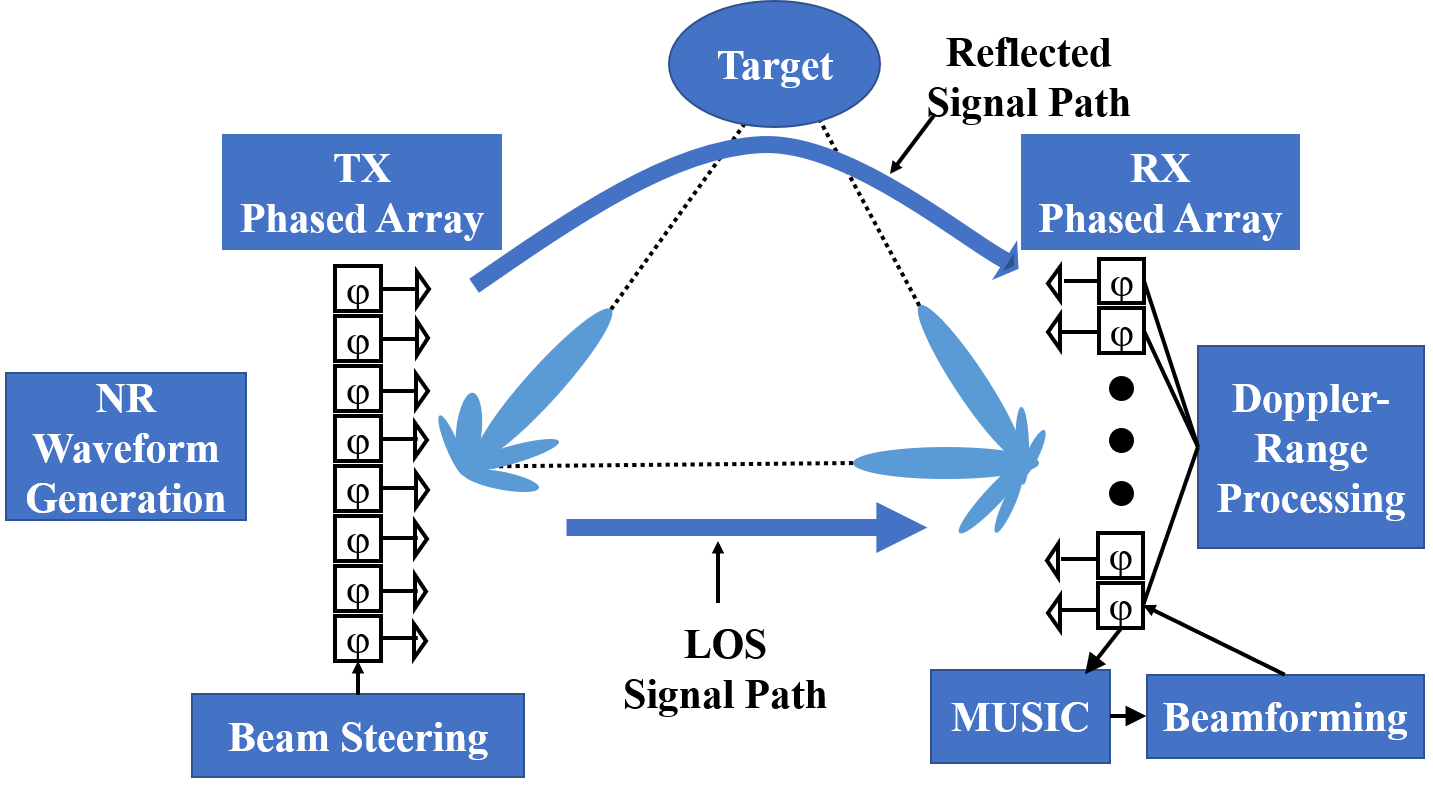
Before real-world deployment, link-level simulations help determine the feasibility of localization solutions. With the help of the Phased Array MATLAB toolbox, we developed a 5G NR compliant test bench to quantify the measurements errors in TDOA and AOA for different bistatic radar configurations in order to evaluate the localization performance of a 5G NR system with radar capabilities, as illustrated in Fig. 3.
Highly directional antenna arrays used at mmWave frequencies have narrower beamwidth; to ensure that the direct signal and the reflected signal are received at the RX with adequate strength, the RX needed to use two RF chains to simultaneously beamform in two directions, one towards the target, and the other towards the TX. An RX with one RF chain which can steer towards only one direction at a time, may first steer towards the TX to receive the direct signal, and then after a fixed time interval (an integral multiple of the periodicity of the reference signal transmission) steer towards the target to receive the reflected signal. The fixed time interval is subtracted from the time at which the reflected signal arrives at the RX to derive the TDOA.
In real-world bistatic radar implementations, the TX antenna array is electrically swept across different steering angles since the direction of the target is not known. However, since this work focuses on quantifying the performance of the radar system and not the performance of the beamsweeping algorithm, we assumed that the TX was steered directly towards the target. The AOAs of the signals at the RX were estimated via the MUSIC algorithm [19, 20].
The TDOA of the direct signal and the reflected signal was estimated via matched filtering, wherein the received waveform was correlated with a time-reversed copy of the transmitted waveform. The TDOA estimate is the time delay between the peaks in the correlation function. To ensure that the reflected signal power of weak targets received using the RX beam directed towards the target was not swamped by the direct signal, a scaled copy of the signal received from the direct path using the RX beam directed towards the TX was removed from the reflected signal received by the RX.
To measure the Doppler shift in the received signal, the NR waveform generated by the TX was repeatedly transmitted as a train of 64 waveforms, which were each passed through a matched filter at the RX. The RX generated a Range-Doppler plot by calculating the discrete Fourier transform (DFT) of the matched filter response of each waveform and determining the common Doppler frequency present in all waveforms [21]. If the Doppler frequency measured by the bistatic radar is , the velocity of the target is given by [14]:
| (22) |
where c is the speed of light and is the carrier frequency. Alternatively, a Kalman filter could be used to track a moving target and estimate the velocity[22].
When radar clutter [6], multipath, and interference from other TXs (currently not modeled in the test bench) are considered, the localization performance will likely be degraded.
IV Performance Evaluation
As described in Section II-A, the target localization algorithms used in this paper rely on two types of measurements — AOA and TDOA. Therefore, we first simulated the error of both measurements using the 5G NR test bench and then used the mean absolute error of the simulated measurements to evaluate the target localization accuracy.
The target position and velocity estimation simulations were conducted at 28 GHz using the DMRS as the reference signal. To emulate target localization in a real NR system, randomly generated data was transmitted along with DMRS (i.e., on resource elements not occupied by DMRS), however it was assumed that the RX had no knowledge of the transmitted data and that the matched filter at the RX was designed to match the DMRS signal alone. A single DMRS symbol was transmitted per time slot (DMRS Additional Position = 0), with six subcarriers utilized per resource block (DMRS Configuration Type-I) [23]. Since no impact was observed by simulating other DMRS configurations (i.e., with different density of DMRS in time or/and frequency), we only present the results with DMRS Configuration Type-I.
A broader antenna beamwidth at the TX compared to the RX ensured that the line-of-sight (LOS) signal path did not fall in a deep antenna null when the TX was steered towards the target. Hence, the TX antenna had 8 while the RX antenna had 16 elements. The maximum effective isotropic radiated power was set to 43 dBm and the RX noise figure was set to 13 dB [24]. A SCS of 120 kHz was chosen for the simulations with a bandwidth of 100 MHz and 400 MHz.
An analysis of the TDOA and AOA errors was conducted for three bistatic scenarios with different bistatic ranges () to simulate different short and mid range bistatic applications, for example, localization for VR gaming, first responders indoors, and vehicles outdoors. Scenario 1 with L = 3 m and m, scenario 2 with L = 15 m and m, and scenario 3 with L = 25 m and m were simulated. Increasing further resulted in very low SNR at the RX node, in which case MUSIC for AOA estimation would fail.
The target was assumed to be isotropic, i.e., a constant bistatic RCS for all orientations. The bistatic RCS of the target was set to -20 dBm2 in scenario 1 in order to model a target with low scattering power (e.g., a person) [25], and 0 dBm2 in scenario 2 and 3 to model a more reflective target (e.g., vehicles) [25]. For localization accuracy evaluation, the target, TX, and RX were assumed to be stationary.
IV-A TDOA and AOA Estimation Errors
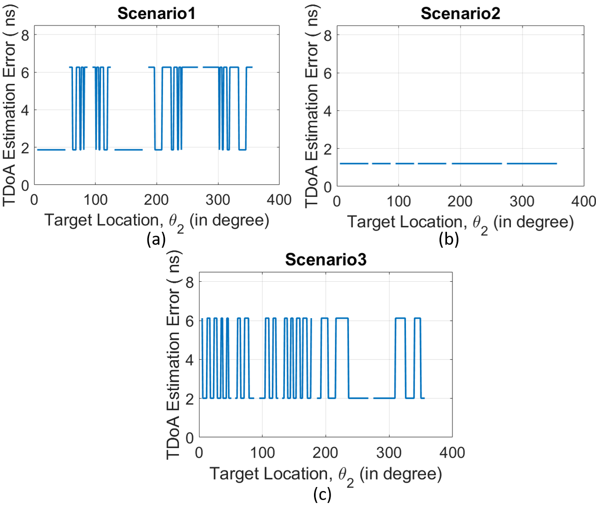
TDOA estimation errors for the three scenarios are plotted in Fig. 4 for different points on the iso-range contour with RF bandwidth of 100 MHz. The main source of error for TDOA measurements was the finite resolution of the measured time. The true TDOA in scenario 1 was 10.0 ns. Due to the finite TDOA resolution of 8.14 ns (assuming an I/Q sampling rate of 122.88 MHz when the signal bandwidth is 100 MHz), at different points on the iso-range contour, the TDOA was estimated to be 8.14 ns or ( =) 16.28 ns (integral multiples of the TDOA resolution), due to which TDOA error oscillated between 1.86 ns and 6.28 ns in Fig. 4(a).
Similarly in scenario 2, the true TDOA is 50 ns, yet the radar estimates the TDOA to be one quantization step below the true value, at ( =) 48.84 ns, due to which an error of 1.16 ns is observed in Fig. 4(b). Finally, in scenario 3, the true TDOA is 83.4 ns which falls between ( =) 81.4 ns and ( =) 89.5 ns, due to which the TDOA error oscillated between 2.0 ns and 6.1 ns in Fig. 4(c).
Increasing the RF bandwidth from 100 MHz to 400 MHz improved the TDOA estimation accuracy as the minimum time resolution improved from 8.14 ns to 2.03 ns. The absolute mean TDOA errors (over the corresponding iso-range contour) were 4.2 ns, 1.21 ns, and 3.55 ns for scenarios 1, 2, and 3, respectively, when a RF bandwidth of 100 MHz was simulated. Increasing the bandwidth to 400 MHz, reduced the absolute mean TDOA errors to 0.17 ns, 1.21 ns, and 0.02 ns.
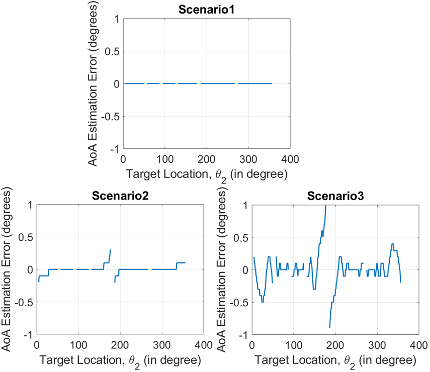
MUSIC was able to very accurately estimate the AOA, as seen in Fig. 5 (with bandwidth of 100 MHz), with sub-degree accuracy achieved at all points on the iso-range contour. As the distance between the target and the nodes increased, the performance of MUSIC deteriorated due to the worsening SNR, however sub-degree accuracy was achieved at all points on the iso-range curve for all three scenarios, with nearly no AOA error for scenario 1 with nodes 3 m apart.
The discontinuities in the error plots of Fig. 4 and 5 occur since the TDOA and AOA could not be measured when the target, the TX and the RX were collinear (at = 90∘, 270∘) as the LOS signal would completely swamp the signal reflected from the target. The boresight of the phased arrays was oriented along the line joining the two nodes. The TDOA and AOA of targets perpendicular to boresight could not be determined due to antenna nulls directed towards the target.
As RF bandwidth was increased from 100 MHz to 400 MHz, a slight decrease in AOA accuracy was observed since the noise power () increased by 6 dB. For example, the absolute mean AOA (over the corresponding iso-range contour) were 0∘, 0.03∘, and 0.16∘ for scenarios 1, 2, and 3, respectively with bandwidth of 100 MHz, which became 0∘, 0.03∘, and 0.23∘, respectively with bandwidth of 400 MHz.
IV-B Utilizing TDOA and AOA estimation errors to evaluate localization performance
To evaluate the target localization performance, the mean absolute AOA and TDOA errors over all points on the iso-range contour were used. The error in the known locations of and was assumed to be 0.01 m. A low error in the TX/RX locations was selected to focus on the effect of errors in AOA and TDOA measurements. The location estimation errors after taking the measurement errors into account were evaluated for all three scenarios via the bistatic localization technique described in Section II-A for both modes of radar operation. By channel reciprocity, the mean absolute measurement errors were equal for both modes of operation.
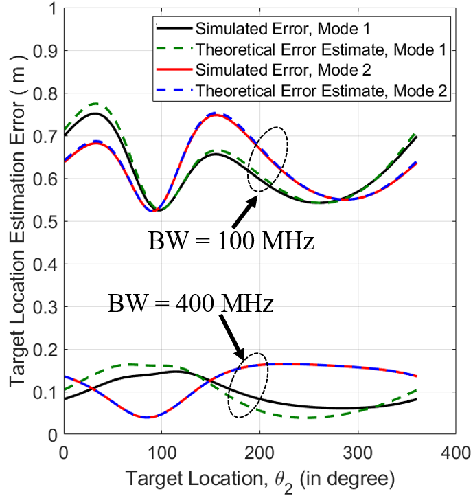
The simulation results for scenario 3 are depicted in Fig. 6, illustrating how the relative distances and angles between the target and the nodes affects the location estimation errors with the same measurement errors, as noted in Section II-B. Although increasing the bandwidth from 100 MHz to 400 MHz slightly decreased the AOA accuracy, the increase in time resolution had a greater impact on position location accuracy, which improved at 400 MHz. In mode 1, the mean localization error dropped from 0.62 m to 0.10 m when the bandwidth was increased from 100 MHz to 400 MHz. In mode 2, the mean localization error dropped from 0.65 m to 0.12 m. The results for the other scenarios follow a similar trend and are omitted due to lack of space. The error predicted from GDOP analysis (using (18)) is also plotted in Fig. 6. As seen in Fig. 6, there is a clear preference of one mode of radar operation over another at different points on the iso-range contour. Since there is very good agreement between the localization error and the error predicted from the GDOP analysis, for a given target location on the iso-range, the GDOP analysis may be used to determine the direction of the transmission ( to or to ) that minimizes the target localization error. Further, if more than two nodes are available for target localization, the set of nodes with lowest predicted GDOP could be selected.
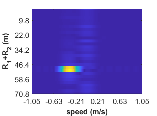
The bistatic radar determined the target velocity with very high accuracy, as illustrated in Fig. 7. The target, located on the iso-range contour at an angle of was moving in the direction normal to the tangent of the iso-range contour, radially inwards at a speed of 0.2 m/s. The velocity estimation error was 0.008 m/s in scenario 3, with a similar performance observed for the other scenarios.
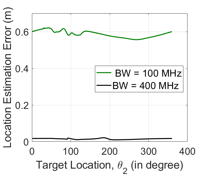
The localization accuracy with the weighted least squares multistatic localization technique described in Section II-C was also evaluated for a multi-static configuration using the mean absolute errors determined from the 5G test bench with system bandwidths of 100 MHz and 400 MHz. One TX node and three RX nodes were used to localize the target. The RX nodes were uniformly placed on a circle with radius centered at the TX. The weighting factors and in (II-C) were set to 1. A comparison of performance of the weighted least squares algorithms in scenario 3 (with a bistatic range of 25 m) is provided in Fig. 8 (similar trend was observed for other scenarios). The mean localization error was 0.58 m and 0.02 m, respectively, when a signal bandwidth of 100 MHz and 400 MHz was used. The results suggest that multistatic localization outperforms bistatic localization, particularly for scenarios with good node geometry (low GDOP) and at wider bandwidths. Hence, the RX must share the measurements (TDOA and AOA) with a central processing unit (e.g., located at the TX), rather than individually calculating a bistatic target estimate. The localization performance was limited by TX-RX location estimation error at 400 MHz (0.01 m), while the performance was limited by the error in the AoA estimates (0.16∘) and TDoA estimates (3.55 ns) at 100 MHz.
V Conclusions and Future Work
With 5G NR, 3GPP has specified operation at mmWave frequencies (FR2). The large available bandwidths in these bands enable both very high data rate communications, and enhanced positioning and localization. This paper focuses on the localization aspect, and provides an analytical method to select the bi/multi-static configuration for a given target location, to minimize the location estimation error. Using simulations with a 5G NR test bench operating at 28 GHz, we evaluated the TDOA and AOA estimation errors for various deployments in ideal channel conditions. We then used the mean TDOA and AOA estimation errors to estimate the target location in a bistatic configuration, for all target locations on the iso-range, and compared it to the analytical prediction. The good alignment between the simulation and the theoretical analysis indicates that GDOP may be used to select the nodes used in the bistatic configuration for target localization.
For example, in a bistatic configuration with = 50 m and baseline L = 25 m, with TDOA and AOA errors derived from the 5G NR simulation, the mean localization error over the iso-range was 0.62 m (0.10 m) with signal bandwidth of 100 MHz (400 MHz). We observed that the minimum TDOA resolution (driven by system bandwidth) limits the localization performance. Lastly, for the same scenario, we showed that the multi-static configuration (using least squares) reduced the localization error to 0.02 m. Future work may include evaluating the performance of other 5G NR reference signals, utilizing other TDOA estimation techniques such as channel estimation based approaches [7], and investigating the effect of radar clutter and multipath on the localization error.
References
- [1] T. S. Rappaport et al., “Wireless Communications and Applications Above 100 GHz: Opportunities and Challenges for 6G and Beyond,” IEEE Access, vol. 7, June 2019.
- [2] O. Kanhere and T. S. Rappaport, “Position Location for Futuristic Cellular Communications: 5G and Beyond,” IEEE Communications Magazine, vol. 59, no. 1, pp. 70–75, 2021.
- [3] T. S. Rappaport, J. H. Reed, and B. D. Woerner, “Position location using wireless communications on highways of the future,” IEEE Commun. Magazine, vol. 34, no. 10, Oct. 1996.
- [4] O. Kanhere and T. S. Rappaport, “Millimeter Wave Position Location using Multipath Differentiation for 3GPP using Field Measurements,” in Proc. IEEE GLOBECOM 2020, Dec. 2020, pp. 1–7.
- [5] F. Liu et al., “Joint Radar and Communication Design: Applications, State-of-the-Art, and the Road Ahead,” IEEE Trans. Commun., vol. 68, no. 6, 2020.
- [6] M. Rahman, J. Zhang, K. Wu, X. Huang, Y. Guo, S. Chen, and J. Yuan, “Enabling Joint Communication and Radio Sensing in Mobile Networks-A Survey,” arXiv preprint arXiv:2006.07559, Sept. 2020.
- [7] Y. Wang, K. Wu, and L. M. Ni, “WiFall: Device-Free Fall Detection by Wireless Networks,” IEEE Trans. Mobile Comput., vol. 16, no. 2, Feb. 2017.
- [8] M. Youssef, M. Mah, and A. Agrawala, “Challenges: device-free passive localization for wireless environments,” in Mobicom, Sept. 2007.
- [9] C. Baquero Barneto et al., “Full-Duplex OFDM Radar With LTE and 5G NR Waveforms: Challenges, Solutions, and Measurements,” IEEE TMTT, vol. 67, no. 10, pp. 4042–4054, Oct. 2019.
- [10] A. Evers and J. A. Jackson, “Analysis of an LTE waveform for radar applications,” in 2014 IEEE Radar Conf., May 2014.
- [11] F. Kong, X, Ren, N. Zheng, G. Chen, and J. Zheng, “A hybrid TOA/AOA positioning method based on GDOP-weighted fusion and its Accuracy Analysis,” in 2016 IEEE IMCEC, Oct. 2016.
- [12] X. Lv, K. Liu, and P. Hu, “Geometry Influence on GDOP in TOA and AOA Positioning Systems,” in 2010 Second Int. Conf. on Networks Security, Wireless Commun. and Trusted Computing, vol. 2, Apr. 2010.
- [13] T. Johnsen, B. Hafskjold, and K. E. Olsen, “Tracking and data fusion in bi- and multistatic radar: a simulation study of geometry dependent uncertainties, filter selection and their influence,” in IEEE Int. Radar Conf., 2005., May 2005.
- [14] H. Kuschel, D. Cristallini, and K. E. Olsen, “Tutorial: Passive radar tutorial,” IEEE Aerosp. and Electron. Syst. Mag., vol. 34, no. 2, 2019.
- [15] C. Liu, J. Yang, and F. Wang, “Joint TDOA and AOA location algorithm,” J. Syst. Eng. and Electron., vol. 24, no. 2, Apr. 2013.
- [16] A. Conti et al., “Soft Information for Localization-of-Things,” Proceedings of the IEEE, vol. 107, no. 11, Nov. 2019.
- [17] S. Al-Jazzar, M. Ghogho, and D. McLernon, “A Joint TOA/AOA Constrained Minimization Method for Locating Wireless Devices in Non-Line-of-Sight Environment,” IEEE Transactions on Vehicular Technology, vol. 58, no. 1, Apr. 2009.
- [18] J. J. Moré, “The Levenberg-Marquardt algorithm: implementation and theory,” in Numerical analysis. Springer, 1978.
- [19] R. Schmidt, “Multiple emitter location and signal parameter estimation,” IEEE Trans. on Ant. and Prop., vol. 34, no. 3, Mar. 1986.
- [20] T. S. Rappaport and J. C. Liberti, Smart Antennas for Wireless CDMA. IEEE Press, 1999.
- [21] D. Koks, “How to create and manipulate radar range-Doppler plots,” DST Organisation Edinburgh (Australia), Tech. Rep., 2014.
- [22] O. Kanhere and T. S. Rappaport, “Outdoor sub-THz Position Location and Tracking using Field Measurements,” in 2021 IEEE International Conference on Communications (ICC), June 2021, pp. 1–6.
- [23] TSG RAN; NR; Physical channels and modulation (Release 16), v16.1.0, 3GPP TS 38.211, March 2020.
- [24] 3GPP, “User Equipment (UE) radio transmission and reception; Part 2: Range 2 Standalone,” TS 38.101-2 V16.4.0, July 2020.
- [25] T. Motomura, K. Uchiyama, and A. Kajiwara, “Measurement results of vehicular RCS characteristics for 79GHz millimeter band,” in 2018 IEEE WiSNet, 2018.