Exploring the effect of streamed social media data variations on social network analysis

Abstract

To study the effects of Online Social Network (OSN) activity on real-world offline events, researchers need access to OSN data, the reliability of which has particular implications for social network analysis. This relates not only to the completeness of any collected dataset, but also to constructing meaningful social and information networks from them. In this multidisciplinary study, we consider the question of constructing traditional social networks from OSN data and then present several measurement case studies showing how variations in collected OSN data affects social network analyses. To this end we developed a systematic comparison methodology, which we applied to five pairs of parallel datasets collected from Twitter in four case studies. We found considerable differences in several of the datasets collected with different tools and that these variations significantly alter the results of subsequent analyses.

Our results lead to a set of guidelines for researchers planning to collect online data streams to infer social networks.

1 Introduction

Online activities can be associated with dramatic offline effects, such as voter fraud misinformation contributing to the 6 January 2020 riots and invasion of the US Capitol building in Washington DC (Scott, 2021), COVID-19 misinformation leading to panic buying of toilet paper (Yap, 2020), online narratives incorrectly attributing Australia’s “Black Summer” bushfires to arson amplifying attention to it in the media (Weber et al., 2020a), and attempts to influence domestic and foreign politics (Ratkiewicz et al., 2011; Woolley, 2016; Morstatter et al., 2018; Woolley and Howard, 2018). For researchers to successfully analyse online activity and provide advice about protection from such events, they must be able to reliably analyse data from online social networks (OSNs).

Social Network Analysis (SNA) facilitates exploration of social behaviours and processes. OSNs are often considered convenient proxies for offline social networks, because they seem to offer a wide range of data on a broad spectrum of individuals, their expressed opinions and inter-relationships. It is assumed that the social networks present on OSNs can inform the study of information dissemination and opinion formation, contributing to an understanding of offline community attitudes. Though such claims are prevalent in the social media literature, there are serious questions about their validity due to an absence of SNA theory on online behaviour, the mapping between online and offline phenomena, and the repeatability of such studies. In particular, the issue of reliable data collection is fundamental. Collection of OSN data is often prone to inaccurate boundary specifications due to sampling issues, collection methodology choices, as well as platform constraints.

Previous work has considered the question of data reliability from a sampling perspective (Morstatter et al., 2013; González-Bailón et al., 2014; Joseph et al., 2014; Paik and Lin, 2015), biases (Ruths and Pfeffer, 2014; Tromble et al., 2017; Pfeffer et al., 2018; Olteanu et al., 2019) and the danger of making invalid generalisations using “big data” approaches lacking nuanced interpretation of the data (Lazer et al., 2014; Tufekci, 2014; Falzon et al., 2017; Venturini et al., 2018). Analyses of incomplete networks exist (Holzmann et al., 2018), but this paper specifically considers the questions of data reliability for SNA, considering not only the significance of online interactions to discover meaningful social networks, but also how sampling and boundary issues can complicate analyses of the networks constructed. Through an exploration of modelling and collection issues, and a measurement study examining the reliability of simultaneously collected, or parallel, datasets, this multidisciplinary study addresses the following research questions:

• To what extent do datasets obtained with social media collection tools differ, even when the tools are configured with the same search settings?

• How do variations in collections affect the results of social network analyses?

Our work makes the following contributions:

1. Discussion of the challenges mapping OSN data to meaningful social and information networks;

2. A methodology for systematic dataset comparison;

3. Recommendations for the use and evaluation of social media collection tools; and

4. Five original social media datasets collected in parallel, and relevant analysis code.

This paper extends Weber et al. (2020b) by including further detail in the methodology, incorporating further analyses and related visualisations and expanding the number of case studies considered from one to four. A discussion section also draws together observations from the case studies and explores ideas for a measure of dataset reliability.

1.1 Paper Overview

This paper continues with five sections: 1) challenges obtaining and modelling social networks from OSN data for SNA: 2) systematic parallel dataset comparison methodology; 3) results from using our methodology in a number of case studies; 4) discussion of our findings and exploration of the notion of a measure of reliability; and 5) recommendations for social media researchers and analysts, plus directions for future research.

2 Social networks from social media

Using SNA to explore social behaviours and processes from OSN data presents many challenges. Most easily accessible OSN data consists of timestamped interactions, rather than details of long-standing relationships, which form the basis of SNA theory. Additionally, although interactions on different OSNs are superficially similar, how they are implemented may subtly alter their interpretation. They offer a window onto online behaviour only, and any implications for offline relations and behaviour are unclear. Beyond modelling and reasoning with the data is the question of collection – accessing the right data to construct meaningful social networks is challenging. OSNs provide a limited subset of their data through a variety of mechanisms, balancing privacy and competitive advantage with openness and transparency.

2.1 Interactions and relationships online

SNA provides concepts and tools to model social relationships among actors. It is based on the premise that an actor’s position in the network impacts their ability to access opportunities and resources and therefore allows us to understand social behaviours and processes in network terms (Borgatti et al., 2013). Given the availability, nature and structure of much OSN data, the use of network-based techniques is a natural choice for the analysis of online social behaviour.

There is, however, an important distinction between the relatively stable, long-term relationships that are typically studied in SNA and the social connections among online actors (Wasserman and Faust, 1994; Nasim, 2016; Borgatti et al., 2009). On social media, accounts can easily fulfil the role of actors, but precisely what constitutes a relationship is unclear. An obvious candidate is the friend or follower relationship common to most OSNs, but, due to how OSNs present their specific features to users, each online community develops its own social relation culture. Therefore, such connections do not necessarily easily translate between OSNs. Is a Facebook friendship really the same as a follow on Twitter, even if reciprocated? And how do each relate to offline friendships?

Table 1: Equivalent social media interaction primitives.

OSN	POST	REPOST	REPLY	MENTION	TAG	LIKE
Twitter	tweet	retweet	reply tweet	@mention	#hashtags	favourite
Facebook	post	share	comment	mention	#hashtag	reactions
Tumblr	post	repost	comment	@mention	#tag	heart
Reddit	post	crosspost	comment	/u/mention	subreddit	up/down vote

OSNs offer ways to establish and maintain relations with others. This is done through interactions, many of which are common between OSNs, such as replying to the posts of others, mentioning others (causing the mentioning post to appear in the mentioned user’s activity feed), using hashtags to reach broader communities, or sharing or reposting another’s post to one’s followers or friends. A sample of interactions with equivalents on different OSNs is offered in Table 1. (N.B. We distinguish interactions from follow or friending actions, which are used to define information flows and are persistent once created, requiring no further manipulation.) Specific interactions may be visible to different accounts, intentionally or incidentally (cf. replying to one post versus using a hashtag). Exploration of these differences may lead to an understanding of the author’s intent and the identity of the intended audience. Is replying to a politician’s Facebook post a way to connect directly with the politician, or is it a way to engage with the rest of the community replying to the post, either by specifically engaging with dialogue or merely signalling one’s presence with a comment of support or dismay? A reply could be all of these things but, in particular, it is evidence of engagement at a particular time and indicates information flow between individuals (Bagrow et al., 2019). Since most online interactions are directed towards a particular individual or group they offer an opportunity to study the flow of information and influence. On the other hand, although friend and follower connections may indicate community membership, they obscure the currency of that connection. Through their dynamic interactions, a user who liked a Star Wars page ten years ago can be distinguished from one who not only liked it, but posted original content to it on a monthly basis. Therefore, we specifically focus on interactions rather than friend and follower relations in this study.

2.2 Social Network Analysis theory

Relationships between individuals in a social network may last for extended periods of time, vary in strength, and be based upon a variety of factors, not all of which are easily measurable. Because of the richness of the concept of social relationships, data collection is often a qualitative activity, involving directly surveying community members for their perceptions of their direct relations and then perhaps augmenting that data with observation data such as recorded interactions (e.g., meeting attendance, emails, phone calls). It is tempting to believe that this richness should be discoverable in the vast amount of interaction data available from OSNs, but there are issues to consider:

1. links between social media accounts may vary in type and across OSNs — it is unclear how they contribute to any particular relationship;

2. what is observed online is only a partial record of interactions in a relationship, where interactions may occur via other OSNs or online media, or entirely offline; and

3. collection strategies and OSN constraints may also hamper the ability to obtain a complete dataset.

Although many interactions seem common across OSNs (e.g., a retweet on Twitter, a repost on Tumblr and a share on Facebook), nuances in how they are implemented and how data retrieved about them is modeled (beyond questions of semantics) may confound direct comparison. For example, a Twitter retweet refers directly to the original tweet, obscuring any chain of accounts through which it passed to the retweeter (Ruths and Pfeffer, 2014). There are efforts to probabilistically regenerate such chains (Rizoiu et al., 2018; Gray et al., 2020), but, in any case, is one account sharing the post further evidence of a relationship? What if it is reciprocated once, or three times? What if the reciprocation occurs only over some interval of time? These questions require careful consideration before SNA can be applied to OSN data.

2.3 Challenges obtaining OSN data

Social media data is typically accessed via an OSN’s Application Programming Interfaces (APIs), which place constraints on how true a picture researchers can form of any relationship. Via its API an OSN can control: how much data is available, through rate limiting, biased or at least non-transparent sampling, and temporal constraints; what types of data are available, through its data model; and how precisely data can be specified, through its query syntax. Many OSNs offer commercial access, which provides more extensive access for a price, though use of such services in research raises questions of repeatability (Ruths and Pfeffer, 2014). This is done to protect users’ privacy but also to maintain competitive advantage. Researchers must often rely on the cost-free APIs, which present further issues. Twitter’s 1% Sample API has been found to provide highly similar samples to different clients and it is therefore unclear whether these are truly representative of Twitter traffic (Joseph et al., 2014; Paik and Lin, 2015). If the samples were truly random, then they ought to be quite distinct, with only minimal overlap. Studying social media data therefore raises questions about the “the coverage and representativeness” (González-Bailón et al., 2014, p.17) of the sample obtained and how it therefore “affects the networks of communication that can be reconstructed from the messages sampled” (González-Bailón et al., 2014, p.17).

Empirical studies have compared the inconsistencies between collecting data from search and streaming APIs using the same or different lists of hashtags. Differences have been discovered between the free streaming API and the full (commercial) “firehose” API (Morstatter et al., 2013). There is general agreement in the literature that the consistency of networks inferred from two streaming samples is greater when there is a high volume of tweets even when the list of hashtags is different (González-Bailón et al., 2014). More concerning is the ability to tamper with Twitter’s sample API to insert messages (Pfeffer et al., 2018), introducing unknown biases at this early stage of data collection (Tromble et al., 2017; Olteanu et al., 2019).

Taking a purely “big data” approach can also lead to inappropriate generalisations and conclusions (Lazer et al., 2014; Tufekci, 2014). This is well illustrated, for example, by the range of motivations behind retweeting behaviour including affirmation, sarcasm, disgust and disagreement (Tufekci, 2014). Similarly, in the study of collective action, there are important social interactions that occur offline (Venturini et al., 2018). Furthermore, relying solely on observable online behaviours risks overlooking passive consumers, resulting in underestimating the true extent to which social media can influence people (Falzon et al., 2017).

OSN APIs provide data by streaming it live or through retrieval services, both of which make use of OSN-specific query syntaxes. Conceptually, therefore, there are two primary collection approaches to consider: 1) focusing on a user or users as seeds (e.g., Gruzd, 2011; Morstatter et al., 2018; Keller et al., 2017) using a snowball strategy (Goodman, 1961) and 2) using keywords or filter terms (e.g., Ratkiewicz et al., 2011; Ferrara, 2017; Morstatter et al., 2018; Woolley and Howard, 2018; Bessi and Ferrara, 2016; Nasim et al., 2018). Focusing on seeds can reveal the flow of information within the communities around the seeds, while a keyword-based collection provides the ebb and flow of conversation related to a topic. These approaches can be combined, as exemplified by Morstatter et al. (2018) in their study of the $2017$ German election: an initial keyword-based collection was conducted for eleven days to identify the most active accounts, the usernames of which were then used as keywords in a six week collection.

Once a reasonable dataset is obtained, there may be benefit in stripping junk content included by automated accounts such as bots (Ferrara et al., 2016; Davis et al., 2016). The question of whether to remove content from social bots (bots that actively pretend to be human) depends on the research question at hand; because humans are easily fooled by social bots (Cresci et al., 2017; Nasim et al., 2018), their contribution to discussions may still be valid (unlike, e.g., that of a sport score announcement bot). Several studies have examined how humans and bots interact, especially within political discussions (Bessi and Ferrara, 2016; Rizoiu et al., 2018; Woolley and Howard, 2018).

So far, the following has been established:

• The OSN information used to form ties in social networks requires careful consideration to ensure meaningfulness; and

• Uncertainty regarding the completeness of OSN data must be acccounted for.

We are now in a position to empirically examine the issue of repeatability, by comparing simultaneously retrieved collections.

3 Methodology

Our initial hypothesis was that if the same collection strategies were used at the same time, then each OSN would provide the same data, regardless of the collection tool used. Consequently, social networks built from such data using the same methodology should be highly similar, in terms of both network and node level measurements. Our methodology consisted of these steps:

1. Conduct simultaneous collections on an OSN using the same collection criteria with different tools.

2. Compare statistics across datasets.

3. Construct sample social networks from the data collected and compare network-level statistics.

4. Compare the networks at the node level.

5. Compare the networks at the cluster level.

Examining the parallel datasets in each of these ways provides the opportunity for the analyst to develop a well-rounded understanding of the participants in an online discussion, their behaviour, how they relate to each other and the communities they form.

3.1 Scope

The scope of this work includes datasets obtained via streaming APIs filtered with keywords. Other collection styles may start with seed accounts, and collect their data and the data of accounts connected to them, either through interaction (e.g., via comments, replies or mentions) or via follower links. Such collections (especially follower networks) often require the collection of data that is prohibitive to obtain, is immediately out of date, and provides no real indication of strength of relationships, as discussed in Section 2.1. Additionally, in the absence of a domain-focused research question to inform the choice of seed accounts, no particular accounts would make sensible seeds, so here we rely on keyword-based collections.

3.2 Data collection

Twitter was chosen as the source OSN due to the availability of its data, the fact that the data it provides was thought to be highly regular (Joseph et al., 2014), and because it has similar interaction primitives to other major OSNs. Twitter is also widely used in academia for research that makes predictions, in particular predictions about population-level events, behavioural patterns and information flows, such as studies of predicting social unrest (Tuke et al., 2020) or misinformation (Wu et al., 2016). The validity of these predictions is fundamentally based on the consistency of the underlying (accessible) data. Two very different collection tools were chosen:

Twarc is an open source library which wraps Twitter’s API, and provided the baseline.

RAPID (Real-time Analytics Platform for Interactive Data Mining) (Lim et al., 2018) is a social media collection and data analysis platform for Twitter and Reddit. It enables filtering of OSN live streams, as well as dynamic topic tracking, meaning it can update filter criteria in real time, adding terms popular in recent posts and removing unused ones.

Both tools facilitate filtering Twitter’s Standard live stream with keywords, providing datasets of tweets as JSON objects.

3.3 Constructing social networks

A social network is constructed from dyads of pair-wise relations between nodes, which in our case are Twitter accounts. The node ties denote intermittent relations between accounts, inferred from observed interactions (Nasim, 2016; Borgatti et al., 2009). Like any choice of knowledge representation, different networks can be constructed to address different research questions. For example, a network to study information flow could draw an arc from node A to B if account B retweets A’s tweet (implying B has read and perhaps agreed with A’s tweet); alternatively, the same interaction could be used to draw an arc from B to A if the relation is to imply an attribution of status or influence (A has influence because B has supported it through a retweet). Networks can be constructed based on direct or inferred relations, including retweeting, replying or mentioning, which we discuss below, or through the shared use of hashtags or URLs, reciprocation or minimum levels of interaction, or friend/follower connections. Morstatter et al. (2018) constructed networks of accounts based on retweets and mentions to discover communities active during the 2017 German election, valuing mentions and retweets equally to mean one account reacting to another. URL sharing behaviour is often studied in the detection and classification of spam and political campaigns (Cao et al., 2015; Wu et al., 2018; Giglietto et al., 2020). Some require more complex calculation such as linking accounts through their participation in detected events (Nasim et al., 2018). Of course, applications for social network analysis exist outside the online sphere, e.g., in narrative analysis (Edwards et al., 2018), and require similar considerations with regard to network design. In the absence of clear alternative research questions, we will examine the social relationships implied by direct interactions and retweet networks (due to their frequency in the literature) and thus we will focus only on the three types of network construction discussed below.

Here, we consider three social networks built from interaction types common to many OSNs: ‘mention networks’, ‘reply networks’, and ‘retweet networks’ (e.g., retweets are analogous to Facebook shares or Tumblr reposts, and replies analogous to comments on posts on Reddit, as shown in Table 1). We define a social network, $G$=$(V,E)$, of accounts $u\in V$ linked by directed, weighted edges $(u_{i},u_{j})\in E$ based on the criteria below.

Mention Networks. Twitter users can mention one or more other users in a tweet. In a mention network, an edge $(u_{i},u_{j})$ exists iff $u_{i}$ mentions $u_{j}$ in a tweet, and the weight corresponds to the number of times $u_{i}$ has mentioned $u_{j}$.

Reply networks. A tweet can be a reply to one other tweet. In a reply network, an edge $(u_{i},u_{j})$ exists iff $u_{i}$ replies to a tweet by $u_{j}$, and the weight corresponds to the number of replies $u_{i}$ has made to $u_{j}$’s tweets.

Retweet networks. A user can repost or ‘retweet’ another’s tweet on their own timeline (visible to their followers). Though retweets are not necessarily direct interactions (Ruths and Pfeffer, 2014), they can be used to determine an account’s reach, and are widely used in the literature (e.g., Vo et al., 2017; Rizoiu et al., 2018; Woolley and Howard, 2018; Morstatter et al., 2018). In a retweet network, an edge $(u_{i},u_{j})$ exists iff $u_{i}$ retweets a tweet by $u_{j}$, and its weight corresponds to the number of $u_{j}$’s tweets $u_{i}$ has retweeted.

Examining networks of the three types built from the same dataset, replies (Figure 1b) are the least common of the three interaction types, and all are dominated by a single large component. Mention networks exhibit relatively high cohesiveness. The similarity between retweets (Figure 1c) and mentions (Figure 1a) is because the data model of a retweet includes a mention of the retweeted account.

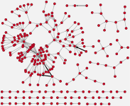
(a) Mentions.

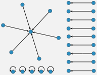
(b) Replies.

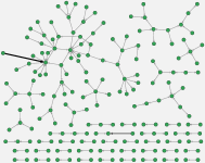
(c) Retweets.

Figure 1: Sample networks of accounts built from 5 minutes of Twitter data. Nodes may appear in one or more networks, depending on their behaviour during the sampled period. The diagrams were constructed with visone (https://visone.info).

3.4 Analyses

At this point, comparative analysis can be applied to the parallel tweet datasets, initially by examining OSN-specific features and then the mention, reply and retweet networks constructed from them. When analysing these networks, it is relevant to note that SNA posits two important axioms on which most network measures are based: network structure affects collective outcomes; and positions within networks affect actor outcomes (Robins, 2015). Furthermore, we should expect minor differences in collections to be amplified in resulting social networks (Holzmann et al., 2018).

3.4.1 Dataset statistics

To compare the parallel datasets we examined a number of features, their frequencies and several maximums. The first of these relate to the absolute count of the following features:

• Tweets: The number of tweets in the corpus.

• Accounts: The number of unique accounts that posted tweets in the corpus (i.e., does not include those that were only mentioned or whose tweets were retweeted).

• Retweets: The number of tweets which were native retweets (i.e., created by clicking the ‘retweet’ button on the Twitter user interface, rather than manually typing in “RT @original_author: original text”, which is another valid, though time consuming, way to post a retweet).

• Quotes: The number of tweets which were quote tweets (non-native retweets, or retweets with comments).

• Replies: The number of tweets which were replies, including replies to tweets outside of the corpus.

• URLs: The number of tweets using URLs, the number of unique URLs used and the number of URL uses.

• Hashtags: The number of tweets using hashtags, the number of unique hashtags used and the number of hashtag uses.

• Mentions: The number of tweets containing mentions of other accounts, the number of unique mentioned accounts, and the number of mentions overall.

The remainder relate to the highest values of the following features:

• Tweeting account: The most prolific account and the number of tweets they posted.

• Mentioned account: The most mentioned account and the number of times they were mentioned.

• Retweeted tweet: The most retweeted tweet and how often it was retweeted.

• Replied-to tweet: The tweet with the most direct replies, and the number of those replies.

• Used hashtags: The first and second most used hashtags, and the number of times they were used.

• URLs: The most used URL, and the number of times it was used.

Based on these figures, we account for major discrepancies between the datasets, which can guide post-processing (e.g., spam filtering). Depending on the application domain, it may be appropriate to also consider comparing the distributions of particular features, rather than just their maximum values.

3.4.2 Network statistics

The following network statistics are used to assess differences in the constructed networks: number of nodes, edges, average degree, density, mean edge weight, component count and the size and diameter of the largest, Louvain (Blondel et al., 2008) cluster count and the size of the largest, reciprocity, transitivity, and maximum k-cores. These measures provide us with an understanding of the ‘shape’ of the networks in terms of how broad and dense they are and the strength of the connections within.

3.4.3 Centrality values

Centrality measures offer a way to consider the importance of individual nodes within a network (Newman, 2010). The centrality measures considered here include: degree centrality, indicating how many other nodes one node is directly linked to; betweenness centrality, referring to the number of shortest paths in the network that a node is on and thus to what degree the node acts as a bridge between other nodes; closeness centrality, which provides a sense of how topologically close a node is to the other nodes in a network; and eigenvector centrality, which measures how connected a node is to other highly-connected nodes. Eigenvector centrality is often compared with Google’s PageRank algorithm (Brin and Page, 1998), which gives a measure of the importance of nodes (e.g., websites) based on references to them by other important nodes or by many nodes. The interested reader is referred to (Robins, 2015; Wasserman and Faust, 1994) for more detail.

Only centrality measures for mention and reply networks are considered, as edges in retweet networks are not direct interactions (Ruths and Pfeffer, 2014).

Given the set of nodes in each corresponding pair of networks is not guaranteed to be identical, it is not possible to directly compare the centrality values of each node, so instead we rank the nodes in each network by the centrality values, take the top $1,000$ from each list, further constrain the lists to only the nodes common to both lists, and then compare the rankings. We initially compare the rankings visually using scatter plots, where a node’s rank in the first and second list is shown on the $x$ and $y$ axes, respectively. A statistical measure of the similarity of the two rankings (of common nodes) is obtained with the Kendall $\tau$ coefficient, with Spearman’s $\rho$ coefficient used as a confirmation measure. To classify the strength of the correlations, we followed the guidance of Dancey and Reidy (2011, p.175), who posit that a coefficient of $0.0-0.1$ is uncorrelated, $0.11-0.4$ is weak, $0.41-0.7$ is moderate, $0.71-0.90$ is strong, and $0.91-1.0$ is perfect.

3.4.4 Cluster comparison

The final step is to consider the clusters discoverable in the mention, reply and retweet networks and compare their membership. We first compare the distribution of the sizes of the twenty largest Louvain clusters (Blondel et al., 2008) visually. The Louvain method was chosen because it works well with large and small networks (Yang et al., 2016) and is used well known in the literature (e.g., Morstatter et al., 2018; Nasim et al., 2018; Nizzoli et al., 2020).

We use the Adjusted Rand index (Hubert and Arabie, 1985) to compare membership. This considers two networks of the same nodes that have been partitioned into subsets. When considered in pairs, there are nodes that appear in the same subset in both partitions ($a$), and there are (many) pairs of nodes that do not appear in the same subsets in either partition ($b$), and the rest appear in the same subset in one of the partitions but not in the other. Defining the total of possible pairings of the $n$ nodes ($\frac{n(n-1)}{2}$) as $c$, the Rand index, $R$, is simply $R=\frac{a+b}{c}$. The Adjusted Rand index (ARI) corrects for chance and provides a value in the range $[-1,1]$ where $0$ implies that the two partitions are random with respect to one another and $1$ implies they are identical.

4 Evaluation Case Studies

Several case studies were conducted to evaluate the comparison methodology, the requirements for which developed progressively, each new case study’s requirements informed by lessons from the previous. The collections varied in the tools used for the parallel collections. As mentioned, Twarc was employed as a baseline, while RAPID was used with topic tracking enabled and disabled, and the tool Tweepy was used in only one case study as a second baseline. The first case study consisted of two parallel Twitter datasets relating to an Australian panel discussion television programme with a prominent online community; the first datasets were collected over the running of the programme (4 hours) and the second covered the following day’s discussion (15 hours), both employing RAPID’s topic tracking feature to broaden the conversation. The second case study examined discussion surrounding Australian Rules Football over a longer period (3 days), without RAPID’s topic tracking. The third also examined the online sports discussion, but over a longer time again (6 days) and only making use of RAPID with no topic tracking. The final case study incorporated a third tool to act as a further baseline and covered a regional but large election day, during which a significant amount of activity was expected. These conditions are summarised in Table 2.

Table 2: Summary of data collection conditions.

Case Study	Collection	Duration	Tool 1	Tool 2	Tool 3
1	Q&A Part 1	4 hours	Twarc	RAPID (topic tracking)	—
	Q&A Part 2	15 hours	Twarc	RAPID (topic tracking)	—
2	AFL1	3 days	Twarc	RAPID (no topic tracking)	—
3	AFL2	6 days	RAPID (no topic tracking)	RAPID (no topic tracking)	—
4	Election	1 day	Twarc	RAPID (with topic tracking)	Tweepy

A summary of the corpora collected is presented in Table 3. As noted above, when topic tracking was employed with RAPID, some of the tweets it collected did not contain any of the initial keywords. These datasets are given the label ‘RAPID-E’. Prior to comparison with the corresponding Twarc datasets, the RAPID-E datasets were filtered to retain only tweets containing at least one of the original keywords. The AFL2 case study used RAPID with no expansion with two sets of Twitter credentials simultaneously; in this case the datasets are labelled ‘RAPID1’ and ‘RAPID2’. A third collection tool, Tweepy, was included in the Election Day case study to act as a second baseline.

Table 3: Summary statistics for the datasets used in this paper.

	Dataset	Tweets	Accounts
Q&A Part 1	Twarc	27,389	7,057
	RAPID	15,930	4,970
	RAPID-E	17,675	5,547
Q&A Part 2	Twarc	15,490	5,799
	RAPID	11,719	4,708
	RAPID-E	23,583	8,854
AFL1	Twarc	44,470	16,821
	RAPID	21,799	11,573
AFL2	RAPID1	30,103	14,231
	RAPID2	30,115	14,232
Election Day	Twarc	39,297	10,860
	Tweepy	36,172	10,242
	RAPID	39,556	10,893
	RAPID-E	46,526	12,696

4.1 Case Study 1: Q&A, #qanda and the effect of topic tracking

Initially, to obtain a moderately active portion of activity, we collected data from Twitter’s Standard live stream relevant to an Australian television panel show, Q&A, that invites its viewers to participate in the discussion live. A particular broadcast in $2018$ was chosen due to the expectation of high levels of activity given the planned discussion topic. As a result, the filter keywords used were ‘qanda’ and two terms that identified a panel member (available on request). We collected two parallel datasets:

Q&A Part 1: Four hours starting $30$ minutes before the hour-long programme, to allow for contributions from the country’s major timezones; and

Q&A Part 2: From 6am to 9pm the following day, capturing further related online discussions.

Twarc acted as the baseline collection as it provides direct access to Twitter’s API, while RAPID was configured to use topic tracking via co-occurrence keyword expansion (Lim et al., 2018), meaning it would progressively add keywords to the original set if they appeared sufficiently frequently (five times in ten minutes). Expanded datasets such as these are referred to as ‘RAPID-E’; it was filtered back to just the tweets containing the original keywords and labelled ‘RAPID’ to enable fair comparison with the ‘Twarc’ dataset. We expected the moderate activity observed would not breach rate limits, and thus RAPID should capture all tweets captured by Twarc. This was not the case.

	Dataset	All	Unique		Retweets		All	Unique
		Tweets	Tweets				Accounts	Accounts
Q&A Part 1	Twarc	27,389	11,481	(41.9%)	14,191	(51.8%)	7,057	2,090	(29.6%)
(20:00-00:00)	RAPID	15,930	22	(0.1%)	8,744	(54.9%)	4,970	3	(0.1%)
	RAPID-E	17,675	1,767	(10.0%)	9,767	(55.3%)	5,547	527	(9.5%)
Q&A Part 2	Twarc	15,490	4,089	(26.4%)	10,988	(70.9%)	5,799	1,128	(19.5%)
(06:00-21:00)	RAPID	11,719	318	(2.7%)	8,051	(68.7%)	4,708	37	(0.8%)
	RAPID-E	23,583	12,180	(51.6%)	13,679	(58.0%)	8,854	4,007	(45.3%)

Table 4: Summary statistics for the Q&A Parts 1 and 2 datasets.

4.1.1 Comparison of collection statistics

The first striking difference between the datasets was the number of tweets collected and the effect on the number of contributors (Table 4). RAPID collected fewer tweets by fewer accounts, but the datasets were close to subsets of the Twarc datasets. Between 26% and 42% of the tweets collected by Twarc were missed by RAPID, but the proportion of retweets in each part is similar (52% and 55% for Part 1 and 69% and 71% for Part 2). In both parts, very few accounts appear in only the RAPID collections. Discussions with RAPID’s developers revealed it dumps tweets that miss the filter terms from the textual parts of tweets (e.g., the body, the author’s screen name, and the author’s profile description). The extra tweets RAPID collected were relevant and in English (based on manual inspection) but posted by different accounts (unique to RAPID-E). Of the tweets that RAPID collected which contained the keywords, they were posted by almost the same accounts as Twarc, but simply did not contain the same tweets.

The benefit of topic tracking via keyword expansion is yet to be strongly evaluated, but this study indicates there are benefits (relevant tweets that omit the original filter terms are picked up once related terms are added) as well as costs (tweets that include the original filter terms but are not collected). RAPID’s expansion strategies are modifiable to optimise data collection, however we chose not to make use of this capability to prevent obscuring the current comparative study. The rest of this analysis explores how much of a difference the keyword expansion makes with regard to SNA.

Table 5: Detailed statistics of Q&A Parts 1 and 2.

	Q&A Part 1		Q&A Part 2
	RAPID	Twarc	RAPID	Twarc
Tweets	15,930	27,389	11,719	15,490
Quotes	325	1,203	498	1,232
Replies	1,446	2,067	1,715	1,731
Tweets with hashtags	10,043	15,591	3,912	3,961
Tweets with URLs	2,470	4,029	3,106	4,074
Most prolific account	Account $a_{1}$	Account $a_{1}$	Account $a_{2}$	Account $a_{3}$
Tweets by most prolific account	103	146	57	68
Most retweeted tweet	Tweet $t_{1}$	Tweet $t_{1}$	Tweet $t_{2}$	Tweet $t_{2}$
Most retweeted tweet count	260	288	385	385
Most replied to tweet	Tweet $t_{3}$	Tweet $t_{3}$	Tweet $t_{4}$	Tweet $t_{4}$
Most replied to tweet count	55	121	58	58
Tweets with mentions	11,314	18,253	10,472	13,514
Most mentioned account	Account $a_{4}$	Account $a_{4}$	Account $a_{4}$	Account $a_{4}$
Mentions of most mentioned account	2,883	3,853	2,753	2,752
Hashtags uses	15,700	23,557	7,672	7,862
Unique hashtags	1,015	1,438	960	1,082
Most used hashtag	#qanda	#qanda	#qanda	#qanda
Uses of most used hashtag	10,065	15,644	2,545	2,549
Next most used hashtag	#auspol	#auspol	#auspol	#auspol
Uses of next most used hashtag	1,381	2,103	1,652	1,349
URLs uses	913	1,650	1,602	2,411
Unique URLs	399	560	658	790
Most used URL	http://wp.me/p2WW3S-Gg	http://wp.me/p2WW3S-Gg	Tweet $t_{5}$ URL	Tweet $t_{6}$ URL
Uses of most used URL	49	128	71	81

Table 6: The top ten most used hashtags in the Q&A datasets (ignoring case and anonymising names).

Q&A Part 1				Q&A Part 2
RAPID		Twarc		RAPID		Twarc
15,930 tweets		27,389 tweets		11,719 tweets		15,490 tweets
Hashtag	Count	Hashtag	Count	Hashtag	Count	Hashtag	Count
qanda	10,065	qanda	15,644	qanda	2,545	qanda	2,549
auspol	1,381	auspol	2,103	auspol	1,652	auspol	1,349
ulurustatement	179	nbn	223	Surname of $a_{4}$	179	Surname of $a_{4}$	179
nbn	178	ulurustatement	187	nbn	135	nbn	133
Surname of $a_{4}$	137	Surname of $a_{4}$	179	breaking	85	ulurustatement	73
marriageequality	125	marriageequality	145	ulurustatement	72	pmlive	71
felizjueves	114	felizjueves	128	qldpol	65	qldpol	64
climate	73	ssm	80	nswpol	65	nswpol	63
8kasımdünyadelilergünü	61	climate	77	pmlive	64	marriageequality	53
ssm	60	libspill	76	marriageequality	53	springst	49

Table 5 reveals that although feature counts vary significantly, many of the most common values are the same (e.g., most retweeted tweet, most mentioned account, most used hashtags). Many are approximately proportional to corpus size (Twarc is 1.72 and 1.32 times larger than RAPID for Parts 1 and 2, respectively), but with notable exceptions and no apparent pattern. Some values are remarkably similar, despite the size of the corpora they arise from being so different. For example, Twarc picked up nearly $8,000$ more hashtag uses than RAPID in Part 1, but fewer than $200$ more in Part 2. Notably, although the most prolific account is different in Part 2, the most mentioned account is the same for both Parts 1 and 2, potentially implying that account has had similarly high influence in both parallel datasets. Furthermore, both datasets shared almost all the same top ten hashtags, though in different orders (see Table 6). Approximately $5,000$ of the extra hashtag uses are of ‘#qanda’. In Part 2, again, the top ten hashtags are nearly the same, but this time the usage counts are similar, except for ‘#auspol’ being used $22\%$ more often in RAPID ($1,652$ times compared with $1,349$), which would account for the overall difference of $190$ uses when combined with the noise of lesser used hashtags. The most used URL in Part 1 is a shortened form of a link to a political party policy comparison resource prepared by an account prominent in the #auspol Twitter discussion. In the longer collection, the most prominent URL is overtaken by retweets, one by @QandA (Tweet $t_{5}$) and one by @SkyNewsAust, an official news media account (Tweet $t_{6}$).

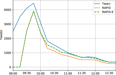
(a) Q&A Part 1.

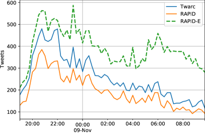
(b) Q&A Part 2.

Figure 2: Twitter activity in the Q&A Parts 1 and 2 dataset over time (in 15 minute blocks).

Moving beyond the bare statistics, the timelines shown in Figures 2a and 2b show the clear differences in tweets retrieved. Though the Twarc and pared back RAPID timelines appear at least proportionately similar, it is firstly notable that the RAPID-E dataset captured so much less data in Part 1 (Figure 2a) and so much more in Part 2 (Figure 2b), particularly from approximately 4 a.m. onwards (UTC). One possible explanation for this is that the discussion on the night of the episode was far more directly focused on the episode themes and had less opportunity to drift to other issues, especially while informed and guided by what was being broadcast at the time. In contrast, those discussing the episode the following day would have had more opportunity to broaden the discussion to other topics, and RAPID’s topic tracking attended to that, apparently at the cost of tweets matching the exact filter terms. Word clouds of the terms drawn from the first and last $5,000$ tweets of the RAPID-E dataset appear to offer mild support for this (Figure 3). Terms are sized according to their frequency. The discussion across the day focuses on the #auspol hashtag, but #qanda is more prominent early on. Mentions of anonymised IDs 1 and 18 are prominent early but shift to ID 6 later. All of these IDS refer to the same individual, but by Twitter handle and first name early on and by surname later in the day. Figure 3c, showing the top terms unique to the evening discussion, indicates that the discussion shifts to humanitarian concerns, perhaps due to events of the day. The early discussion (Figure 3a) seems to mention individuals much more than later, as indicated by the greater size of anonymised IDs. This fact alone implies that the early discussion was focused more directly on the the Q&A episode, as the topics it covered related to particular relationships and events involving those individuals.

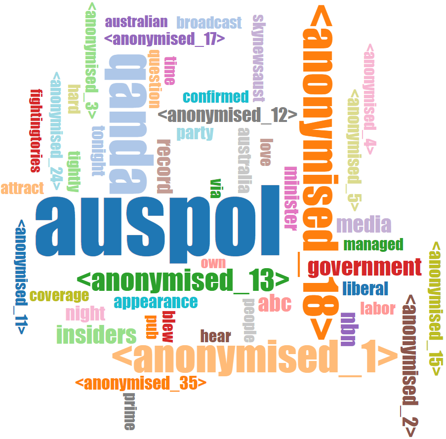
(a) From the first 5000 tweets.

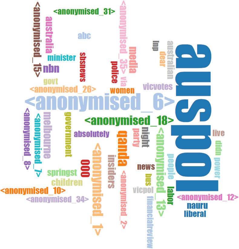
(b) From the last 5000 tweets.

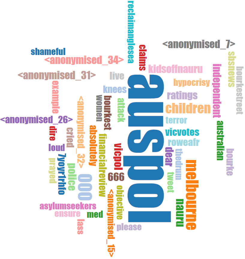
(c) Unique to the last 5000 tweets.

Figure 3: Word clouds of the $50$ most used terms (anonymised) in the first and last $5,000$ tweets of the Q&A Part 2 RAPID-E dataset, and the top $50$ terms unique to the last $5,000$ tweets.

The second notable feature is that the RAPID tool appeared to miss many of the available tweets in the first half an hour of the Part 1 collection. RAPID-E’s first half hour includes only six tweets, the first of which was at 9 a.m. (UTC), while RAPID’s only includes four tweets, the first of which was at 9:15 a.m. It is unclear why the tool missed the tweets that Twarc captured, but a discrepancy such as this suggests it was not by design. The reason that the RAPID-E included tweets without the key terms early on in the specified timeframe is that the collection was running prior to the cut-off at 9 a.m. (UTC), tracking topics while it ran, as a ‘burn-in’ period, and we have extracted just these specific periods (UTC 0900 to 1300, and UTC 1900 to 1000 the next day) to study, post collection.

4.1.2 Comparison of network statistics

Given the differences in datasets, we expect differences in the derived social networks (Tables 7 and 8) (Holzmann et al., 2018). We also present the proportional balance between each dataset’s statistics in Figures 4 and 5. Each network is dominated by a single large component, comprising over 90% of nodes in the retweet and mention networks, and around 70% in the reply networks. The distributions of component sizes appear to follow a power law, resulting in corresponding high numbers of detected clusters.

Table 7: Q&A Part 1 network statistics.

	RETWEET		MENTION		REPLY
	RAPID	Twarc	RAPID	Twarc	RAPID	Twarc
Nodes	3,234	4,426	4,535	6,119	1,184	1,490
Edges	7,855	12,327	13,144	19,576	1,231	1,631
Average degree	2.429	2.785	2.898	3.199	1.040	1.095
Density	0.001	0.001	0.001	0.001	0.001	0.001
Mean edge weight	1.113	1.151	1.268	1.300	1.175	1.267
Components	74	95	86	108	164	192
Largest component	3,061	4,115	4,326	5,819	829	1,081
- Diameter	12	12	10	11	15	15
Clusters	93	115	109	134	186	219
Largest cluster	318	540	731	1,348	169	229
Reciprocity	0.004	0.007	0.025	0.025	0.106	0.099
Transitivity	0.026	0.034	0.065	0.063	0.024	0.021
Maximum k-core	11	14	13	16	2	3

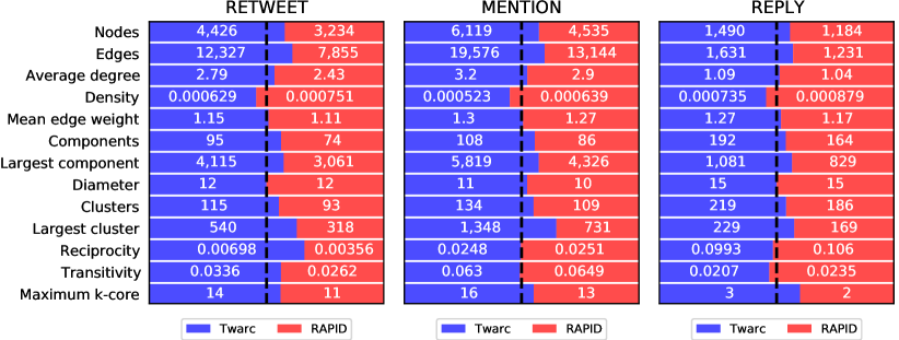
Figure 4: The proportional balance between Twarc and RAPID statistics of the retweet, mention and reply networks built from the Q&A Part 1 datasets.

Table 8: Q&A Part 2 network statistics.

	RETWEET		MENTION		REPLY
	RAPID	Twarc	RAPID	Twarc	RAPID	Twarc
Nodes	3,594	4,591	5,198	6,205	1,492	1,507
Edges	7,344	10,110	14,802	18,184	1,560	1,576
Average degree	2.043	2.202	2.848	2.931	1.046	1.046
Density	0.001	0.000	0.001	0.000	0.001	0.001
Mean edge weight	1.096	1.087	1.245	1.222	1.099	1.098
Components	118	176	123	179	196	201
Largest component	3,308	4,085	4,854	5,612	1,073	1,080
- Diameter	12	11	10	10	15	15
Clusters	138	197	158	210	221	226
Largest cluster	471	727	1,090	1,513	122	123
Reciprocity	0.004	0.004	0.024	0.025	0.072	0.071
Transitivity	0.027	0.026	0.084	0.079	0.016	0.016
Maxmium k-core	9	10	11	14	3	3

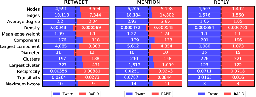
Figure 5: The proportional balance between Twarc and RAPID statistics of the retweet, mention and reply networks built from the Q&A Part 2 datasets.

Network structure statistics like density, diameter (of the largest component in disconnected networks), reciprocity and transitivity may offer insight into social behaviours such as influence and information gathering. The high component counts in all networks lead to low densities and correspondingly low transitivities, as the potential number of triads is limited by the connectivity of nodes. That said, the largest components were consistently larger in the Twarc datasets, but the diameters of the corresponding largest components from each dataset were remarkably similar, implying that the extra nodes and edges were in the components’ centres rather than on the periphery. This increase in internal structures improves connectivity and therefore the number of nodes to which any one node could pass information (and therefore influence) or, at least, reduces the length of paths between nodes so information can pass more quickly. The similarities in transitivity imply the increase may not be significant, however, with networks of these sizes. Reciprocity values may provide insight into information gathering, which often relies on patterns of to-and-fro communication as a person asks a question and others respond. Interestingly, the only significant difference in reciprocity is in the Part 1 retweet networks, with the Twarc dataset having a reciprocity nearly double that of the RAPID dataset (though still small). The Twarc dataset includes 60% more retweets than the corresponding RAPID dataset and 40% more accounts (Table 4), which may account for the discrepancy. Given the network sizes, the reciprocity values indicate low degrees of conversation, mostly in the reply networks. Interestingly, mean edge weights are very low ($1.3$ at most), implying that most interactions between accounts in all networks happen only once, despite these being corpora of issue-based discussions.

The proportional statistical differences between the corresponding datasets are highlighted in Figure 4 for Part 1 and Figure 5 for Part 2. Part 1’s Twarc networks were larger, both in nodes and edges, but less dense, than the RAPID ones, and the largest component in each network is larger by a significant proportion of the extra nodes (it is not clear what portion of the extra nodes are members of the largest components, however). An increase in components also led to an corresponding increase in detected clusters, and an increase in the size of the largest detected cluster. As mentioned earlier, the increase in internal structures leads to a higher maximum k-core value. Though the proportional differences in reciprocity in the retweet networks are high, the values themselves remain low. Part 2’s reply networks are remarkably similar despite the Twarc dataset having $26\%$ more tweets. The differences in Part 2’s retweet and mention networks are similar to those of Part 1.

That the differences in retweet and mention networks are so proportionately similar across both Parts 1 and 2 is notable because the retweet network is not based on direct interactions, while the mention network is. Retweeting a tweet links a retweeter, X, back to the original author, Y, of a tweet, rather than any intermediate account, even if the retweet passed through several accounts on its way between Y and X. It is possible that these datasets were sufficiently constrained both in size and timespan and focus of the participants (by which we mean they engaged in the discussion by following the #qanda hashtag), that there was little opportunity to build up chains of retweets.

Next we look at two major categories of network analysis: indexing, for the computation of node-level properties, such as centrality; and grouping, for the computation of specific groups of nodes, such as clustering.

4.1.3 Comparison of centralities

Centrality measures can tell us about the influence an individual has over their neighbourhood, though the timing of interactions should ideally be taken into account to get a better understanding of their dynamic aspects (e.g., Falzon et al. 2018). If networks are constructed from partial data, network-level metrics (e.g., radius, shortest paths, cluster detection) and neighbourhood-aware measures (e.g., eigenvector and Katz centrality) may vary and not be meaningful (Holzmann et al., 2018).

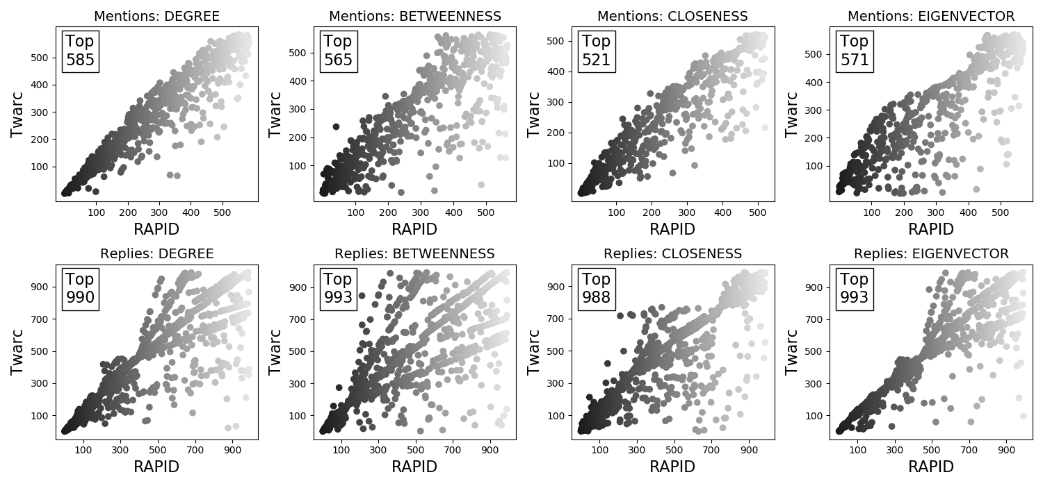
(a) Q&A Part 1.

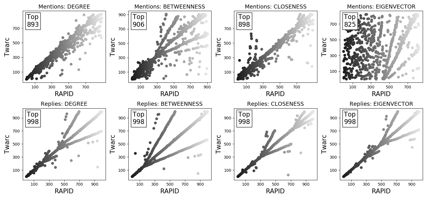
(b) Q&A Part 2.

Figure 6: Centrality ranking comparison scatter plots of the mention and reply networks built from the Q&A Parts 1 and 2 datasets. In each plot, each point represents a node’s ranking in the RAPID and Twarc lists of centralities (common nodes amongst the top $1,000$ of each list). The number of nodes appearing in both lists is inset. Point darkness indicates rank on the $x$ axis (darker = higher).

We compare centralities of corresponding networks using scatter plots of node rankings, as per Section 3.4 (Figure 6). The symmetrical structures come from corresponding shifts in order: if an item appears higher in one list, then it displaces another, leading to the evident fork-like patterns. There is considerable variation in most centrality rankings for both mention and reply networks in Part 1 (Figure 6a) but much less in Part 2 (Figure 6b), apart from the ranking of eigenvector centralities for the mention networks, which lacks almost any alignment between the RAPID and Twarc node rankings, despite the high number of common nodes ($825$). This implies that the neighbourhoods of nodes differ between the Twarc and RAPID mention networks, but the top ranked nodes are similar though their orders differ greatly. Furthermore, the relatively few common nodes in Part 1’s Twarc mention networks ($521$ to $585$) and greater edge count (Tables 7) could indicate that the extra edges significantly affect the node rankings. However, Part 2’s Twarc mentions networks also had many more edges, but many more nodes in common (approximately $900$). Thus it must have been how the mentions were distributed in the datasets that differed, rather than simply their number. It is not clear that Part 1’s four hour duration (cf. Part 2’s $15$ hours) explains this. Instead, if we look at the $11,480$ tweets unique to Twarc in Part 1 (cf. fewer than $4,000$ are unique to Twarc in Part 2, Table 4), only $622$ are replies, whereas $6,915$ include mentions. There are also $34\%$ more unique accounts in the Part 1 Twarc dataset, but only $19\%$ more in the Part 2 Twarc dataset (Table 4). Each mention refers to one of these accounts and forms an extra edge in the mention network, thus altering the network’s structure and the centrality values of many of its nodes; this is likely where the variation in rankings originates.

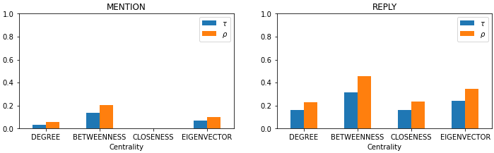
(a) Q&A Part 1.

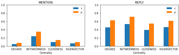
(b) Q&A Part 2.

Figure 7: Centrality ranking comparisons using Kendall $\tau$ and Spearman’s $\rho$ coefficients for corresponding mention and reply networks made from the Q&A Parts 1 and 2 datasets.

The Kendall $\tau$ and Spearman’s $\rho$ coefficients were calculated comparing the corresponding lists of nodes, each pair ranked by one of the four centrality measures (Figure 7). Although somewhat proportional, it is notable how different the coefficient values are, especially in Part 2. While Twarc produced more tweets than RAPID (Table 4), and more unique accounts, the corresponding mention and reply node counts are not significantly higher (Tables 7 and 8). In fact, the node counts in the Part 1 reply networks are correspondingly lower than in the Part 2 reply networks, even though both Part 2 datasets were smaller. Edge counts in the mention networks were very different (Twarc had many more) but were quite similar in the reply networks.

The biggest variation was in the mention networks from Part 1 (Figure 6a and Table 7), due to the large number of extra mentions from Twarc. It is notable that the Kendall’s $\tau$ was low for all mention networks (Figure 7), especially for degree and closeness centrality. It is worth noting the minor differences in the degree and immediate neighbours of nodes impacts degree and closeness centralities significantly, and, correspondingly, their relative rankings. In contrast, rankings for betweenness and eigenvector centrality, which rely more on global network structure, remained relatively stable.

4.1.4 Comparison of clusters

We finally compare the networks via largest clusters (Figure 8). The reply network clusters are relatively similar, and the largest mention and reply clusters differ the most. The ARI scores (Table 9) confirm that the reply clusters were most similar for Parts 1 and 2 ($0.738$ and $0.756$, respectively), possibly due to the small size of the reply networks. The mention and retweet clusters for Part 2 were more similar than those of Part 1 ($0.437$ and $0.468$ compared to $0.320$ and $0.350$), possibly due to the longer collection period. In Part 1, there is a chance the networks are different due to RAPID’s expansion strategy. Changes to filter keywords may have collected posts of other vocal accounts not using the original keywords, at the cost of the posts which did.

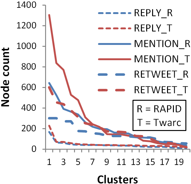
(a) Q&A Part 1.

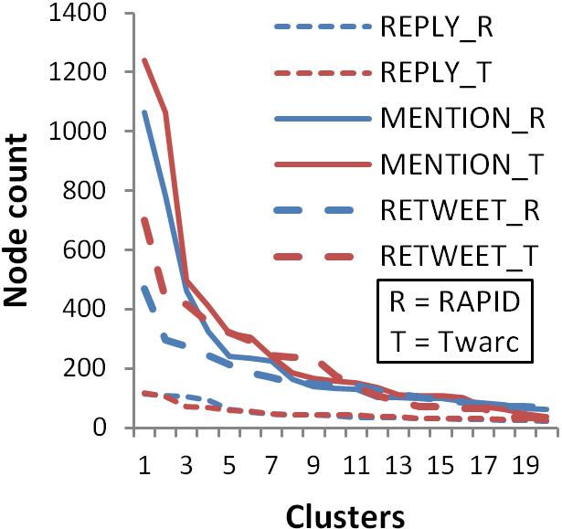
(b) Q&A Part 2.

Figure 8: The largest retweet, mention and reply clusters built from the Q&A Parts 1 and 2 datasets.

	RETWEET	MENTION	REPLY
Q&A Part 1	0.320	0.350	0.738
Q&A Part 2	0.437	0.468	0.756

Table 9: Adjusted Rand index scores for the clusters found in the corresponding retweet, mention and reply networks built from the Q&A Parts 1 and 2 datasets.

4.1.5 Summary of findings

Overall, Twarc and RAPID provided very different views into the Twitter activity surrounding the Q&A episode in question, both on the evening of and the day after. This includes variations in basic collection statistics, network statistics for retweet, mention and reply networks built from the collected data, centrality measures of the nodes in the networks and comparison of detected clusters. The extra tweets collected by the Twarc collections appear to have resulted in greater numbers of connections internal to the largest components, which may have implications for the analysis of influence, as reachability correspondingly increases. Deeper study of reply content is required to inform patterns of information gathering.

We are left with the open question of how reliable social media can be as a data source, if conducting simultaneous collection activities with the same query criteria can provide such different networks. Is the variation due to the platform providing a random sample of the overall data or an effect of the tool being used?

We next considered a more tightly controlled comparison of Twarc and RAPID, disabling RAPID’s expansion strategies so that the tools performed as similarly as possible.

4.2 Case Study 2: A weekend of AFL without topic tracking

RAPID’s topic tracking feature broadens the scope of of the collection at the cost of strictly matching tweets, resulting in distinctly different corresponding corpora. Although the rankings of the most central nodes in networks built from the corpora appear relatively stable, the question remains of why the corpora were so different in size. In this section, we discuss a case study in which we disabled RAPID’s topic tracking feature, expecting the resulting corresponding corpora to increase in similarity, especially over a longer period collection. Figure 9 indicates that again, initially at least, it appeared that Twarc and RAPID produced very different, but proportional over time, datasets. Constraining the datasets to only those tweets with a “lang” property of “en” or “und” resulted in much more similar datasets.

Table 10: Summary dataset statistics of the AFL1 collection.

Dataset	All	Unique		Retweets		All	Unique
	Tweets	Tweets				Accounts	Accounts
Twarc	44,461	22,731	(51.1%)	11,482	(25.8%)	16,821	5,274	(31.4%)
RAPID	21,799	69	(0.3%)	7,047	(32.3%)	11,573	26	(0.2%)
Twarc-en	25,231	4,065	(16.1%)	8,531	(33.8%)	12,399	1,187	(9.6%)
RAPID-en	21,235	69	(0.3%)	6,849	(32.3%)	11,238	26	(0.2%)

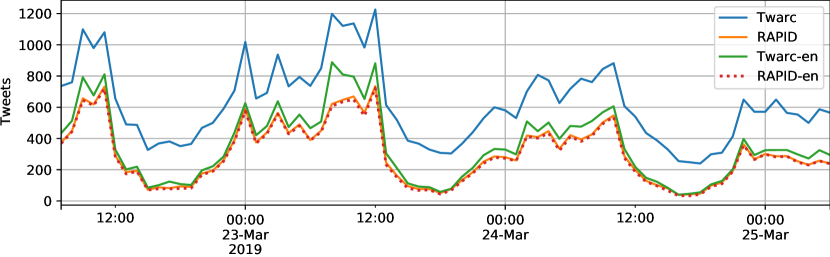
Figure 9: Twitter activity in the AFL1 dataset over time (in 60 minute blocks).

4.2.1 Comparison of collection statistics

We conducted two parallel collections under the term “afl” over a three day period in March 2019 using RAPID without topic tracking and Twarc. This collection is labelled “AFL1” in Tables 2 and 3 and further detail is offered in Table 10. The datasets obtained appear to be dramatically different: RAPID collected just shy of 22k tweets while Twarc found approximately twice that number with around 45k tweets, with 21,730 in common. Interestingly, as can be seen in Figure 9, the extra tweets appear to occur relatively evenly and consistently over time, rather than spiking. On closer inspection, it became apparent that the balance in languages was different, with 36% of the Twarc collection having lang property of ‘jp’ (Japanese) and 52% ‘en’ (English), while RAPID consisted of 94% English tweets (Figure 10). When both collections were trimmed to tweets with a lang property of ‘en’ or ‘und’ (undefined), they reduced to $25,231$ tweets (Twarc) and $21,235$ tweets (RAPID), with 21,166 in common, which still leaves more than 4,000 tweets specific to Twarc (Figure 11). Twitter populates this field based on a variety of factors including the account’s preferred language but also on built-in language detection facilities, with varying degrees of success. The “AFL1” dataset, reduced to only posts with a lang property of ‘en’ or ‘und’ is referred to as “AFL1-en” henceforth.

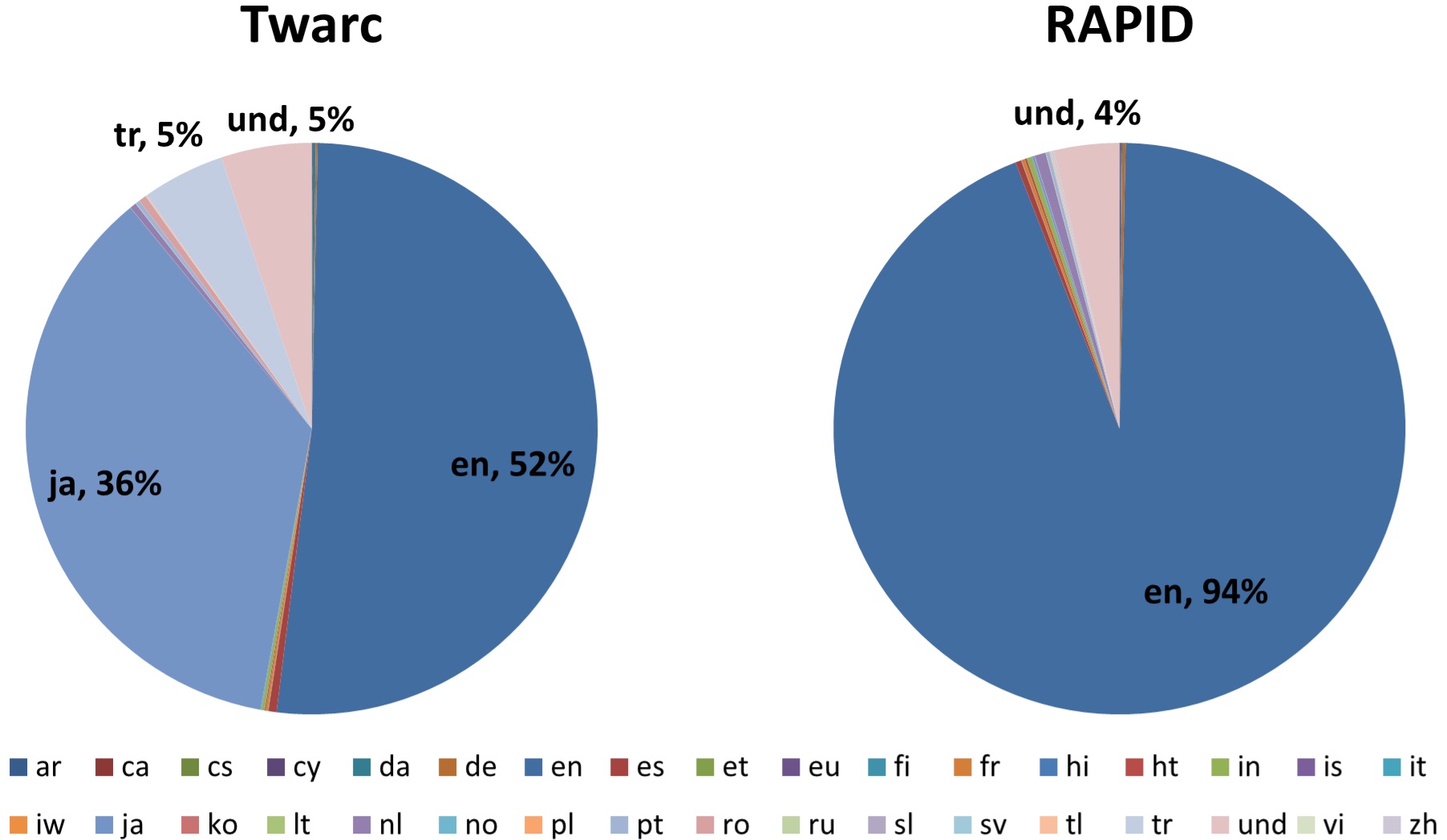
Figure 10: Language distributions of the RAPID and Twarc collections using the filter term “afl”.

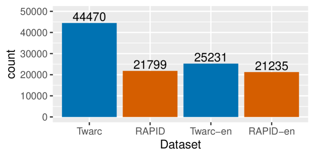
Figure 11: Tweet counts from the RAPID and Twarc collections using the filter term “afl”.

As previously mentioned, RAPID does not retain tweets which do not contain filter terms in text-related portions of the tweets. In the Twarc collection, the term ‘afl’ appeared in the domain of a website that many of the Japanese tweets referred to, belonging to an online marketplace. These tweets were dropped by RAPID and did not appear in the final collection.

Only $69$ tweets were unique to the RAPID AFL1-en dataset, and they appear to be AFL-related sports discussions. The $4,065$ tweets unique to the Twarc dataset comprise $2,595$ English tweets and $1,470$ with “und” for the lang value. This field is populated by Twitter based on language detection algorithms. When a language cannot be detected, such as when there is not sufficient free text to analyse, the value “und” is used. Inspection of the tweets indicates the reason for this: the undefined tweets include $884$ retweets, $1,366$ tweets with URLs, $116$ with hashtags, and $916$ with mentions. Of the “und” tweets with URLs, the vast majority ($1,188$) refer to a Japanese online electronics marketplace ($771$) and a Japanese online media platform ($417$). The next largest group refer to $38$ retweets, some of the official @AFL account ($9$), though there are $16$ and $5$ retweets of two accounts that Botometer (Davis et al., 2016) scored at $4.2$ and $4.4$ out of $5$, respectively, as bot-like, and both refer to the previously mentioned Japanese electronics marketplace. The top $12$ most used hashtags in the English subset relate to the AFL, while the top $14$ for the “und” subset are all Japanese terms, except for “iphone” (at number 9). The top term (in Japanese) is the name of the marketplace. The English tweets are mostly related to the AFL, though there is considerable obvious content from bot-like accounts, with several accounts posting the same content (offers of live streams of the matches) repeatedly within a short space of time (their messages appear adjacent in the timeline).

Property	Twarc-en	RAPID-en
Tweets	25,231	21,235
Accounts	12,399	11,238
Retweets	8,531	6,849
Quotes	2,291	1,615
Replies	6,185	5,936
Tweets with hashtags	7,606	6,911
Tweets with URLs	10,266	7,345
Most prolific account	Account $a_{5}$	Account $a_{5}$
Tweets by most prolific account	363	362
Most retweeted tweet	Tweet $t_{5}$	Tweet $t_{5}$
Most retweeted tweet count	529	529
Most replied to tweet	Tweet $t_{6}$	Tweet $t_{6}$
Most replied to tweet count	141	141
Tweets with mentions	17,467	15,230
Most mentioned account	Account $a_{6}$	Account $a_{6}$
Mentions of most mentioned account	7,131	7,130
Hashtag uses	17,352	15,886
Unique hashtags	2,381	2,249
Most used hashtag	#afl	#afl
Most used hashtag count	4,523	4,522
Next most used hashtag	#aflpiescats	#aflpiescats
Uses of next most used hashtag	1,575	1,482
URL uses	6,557	3,552
Unique URLs	2,843	2,043
Most used URL	http://watchrugby.net/AFL/	http://watchrugby.net/AFL/
Uses of most used URL	494	251

Table 11: Statistics of the AFL1-en RAPID and Twarc datasets.

Once reduced to a relatively comparable state, the “AFL1-en” parallel datasets can be examined in more detail. It is understood that the tweets they consist of will differ, given that rate-limiting constraints may have caused each to receive different tweets. The statistics in Table 11 bear this out with the Twarc dataset statistics being approximately proportionately larger when compared with the RAPID dataset statistics. The author IDs have been anonymised, but the most mentioned account is the official @AFL account, while the most prolific author appears to be automated to some degree, having posted nearly $35,000$ tweets in two years and a Botometer (Davis et al., 2016) Complete Automation Probability (CAP) of $68\%$, many seemingly promote the AFL, tennis, and a singer. The most replied to tweet was posted by an Australian NBA player and the most retweeted tweet was of an amusing video of an AFL supporter.

4.2.2 Comparison of network statistics

	RETWEET		MENTION		REPLY
	RAPID-en	Twarc-en	RAPID-en	Twarc-en	RAPID-en	Twarc-en
Number of nodes	5,584	6,430	11,566	12,525	4,705	4,759
Number of edges	5,881	6,977	22,310	23,937	4,928	5,005
Average degree	1.053	1.085	1.929	1.911	1.047	1.052
Density	0.000	0.000	0.000	0.000	0.000	0.000
Mean edge weight	1.165	1.223	1.308	1.329	1.205	1.236
Components	494	536	666	713	791	798
Largest component	3,946	4,233	9,416	9,789	2,951	3,017
- Diameter	16	16	17	17	16	16
Clusters	544	579	736	781	861	863
Largest cluster	659	753	2,177	2,125	851	844
Reciprocity	0.004	0.005	0.057	0.055	0.139	0.131
Transitivity	0.035	0.038	0.143	0.152	0.039	0.034
Maximum k-core	4	4	9	11	4	4

Table 12: Comparative statistics for networks generated from the RAPID and Twarc datasets for the ALF1-en collection.

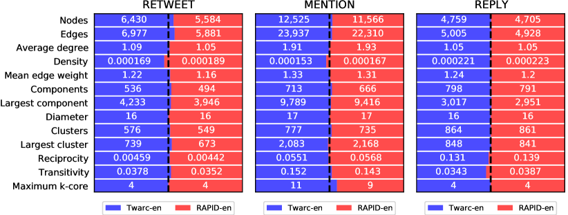
Figure 12: The proportional balance betweet Twarc and RAPID statistics of the retweet, mention and reply networks built from the AFL1-en datasets.

The network statistics Table 12 indicate that the networks were much more similar than in the Q&A case study, though there are still notable differences. The largest components of the retweet, mention and reply networks are, at most, 15% larger by node count, and the largest components are correspondingly similar, though their diameters and densities indicate they are much more sparse than the corresponding Q&A ones, with corresponding implications for the opportunity to influence. In contrast, in sporting discussions, there is less motivation to attempt to convert fellow sports fans to cheer for one’s team than there is in a political discussion. Certainly in this study, politics has tended to generate more discussion than sports in general, and the nature of the discussions is also different. The reciprocity values here are much higher than in the Q&A case study, implying the presence of more communication among the communities that do exist. Another difference that lends weight to this interpretation is the average degree of nodes in the networks. In the Q&A retweet and mention networks, the average degrees were around 2-2.5 and 3, respectively, implying some repetition in connectivity, whereas in the sporting discussing the average degrees are around 1 and 2, respectively, implying much less continued interaction. As indicated in Figure 12, the degree values of the Twarc and RAPID networks are highly similar.

The number of tweets and accounts in the AFL1-en datasets (Table 11), coupled with the number of nodes and edges in the derived mention and reply networks (Table 12), indicate that although the AFL1-en collections differed by nearly $4,000$ tweets, the number of accounts was not significantly different (approximately $10\%$ more in Twarc) with a corresponding increase in nodes and edges in the mention network (8.3% and 7.3%, respectively) but only $54$ and $77$ (1.1% and 1.6%, respectively) more in the reply network.

4.2.3 Comparison of centralities

Considering the similarity of interaction networks constructed from the respective AFL1-en datasets, we compare the relative ranking of the the top network nodes by various centrality values (with an upper bound of $1,000$ nodes). Figure 13 shows scatterplots of the relative rankings of nodes common to corresponding networks, and Figure 14 plots the Kendall Tau and Spearman’s coefficients of the corresponding relative rankings. As with the Q&A collection, the centrality of nodes in the reply networks show more similarity than those in the mention networks, which is likely due to their relative size; Table 12 indicates a significant discrepancy in the reply and mention network sizes and average degree. Closeness is notably low in similarity, though the high component count would account for that. It is apparent the the most central nodes in both network types mostly maintain their ordering for the first several hundred nodes, but all begin to diverge at some point. A few isolated nodes change their ranking significantly, such as those in the top left of the mentions betweenness and closeness plots, degrading their rankings (appearing above the diagonal), and those in the reply closeness and eigenvector plots, improving their rankings (appearing below the diagonal), but the majority diverge in a trident pattern, implying lower ranked nodes improve their rankings swapping out higher ranked nodes at progressively greater distances. The reason for the consistency is unclear. Minor variations would ensure that nodes’ centrality values varied and thus their rankings could easily vary significantly, especially due to the high number of components. The high K-core values for the mention networks are likely to explain the high betweenness and eigenvector centrality values, as the highest ranked of these will reside in the larger components, which will have the greater likelihood of being similar across the networks.

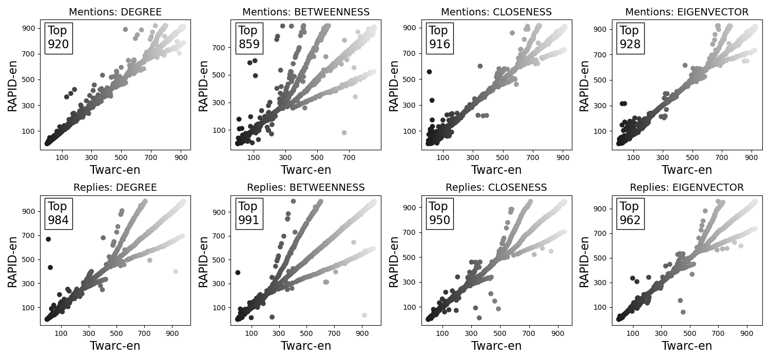
Figure 13: Centrality ranking comparison scatter plots of the mention and reply networks built from the AFL1-en datasets. In each plot, each point represents a node’s ranking in the RAPID-en and Twarc-en lists of centralities (common nodes amongst the top $1,000$ of each list). The number of nodes appearing in both lists is inset. Point darkness indicates rank on the $x$ axis (darker = higher).

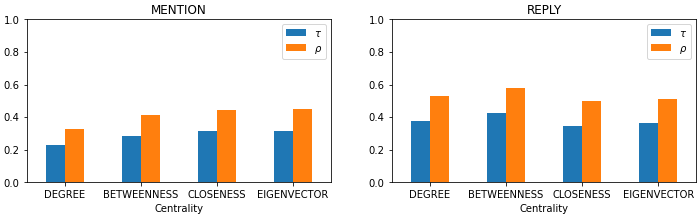
Figure 14: Centrality ranking comparisons from the RAPID and Twarc datasets of the AFL1-en collection using Kendall Tau scores and Spearman’s Coefficients.

4.2.4 Comparison of clusters

Comparing the clusters detected with the Louvain method (Blondel et al., 2008) in the retweet, mention and reply networks results in ARI values in Table 13. This implies that although the networks consisted of many components, the clusters they formed were highly similar for retweet and reply networks, and only slightly less so for the mention networks, despite the fact that the Twarc mention network included more than $2,000$ more mention edges.

RETWEET	MENTION	REPLY
0.818	0.675	0.853

Table 13: Adjusted Rand index scores for the clusters found in the networks built from the RAPID and Twarc datasets for the AFL1-en collection.

4.2.5 Summary of findings

This case study makes it clear that the tool used for collection can have a significant effect on the data collected and the resulting analytic results. It was serendipitous that the filter term chosen was “afl”, because a more specific term or set of terms is unlikely to have captured the non-English content that Twarc did. This highlighted the fact that RAPID was post-processing and filtering the tweets it collected, and raises general questions for social media data collection: Do other collection tools, especially commercial ones, do this post-processing too, as a “convenience” or “value-add” to their users? Do they make it clear if and when they do? The validity of evidence-based conclusions rests on these details. Even when both datasets were filtered to ensure some degree of consistency, there remained large differences in the networks constructed from them. Minor differences in datasets may result in amplified differences in analyses.

A further, even more fundamental, question remained after this case study, which is addressed by the next subsection: Does the same tool provide the same data over two simultaneous collections with identical filter terms?

4.3 Case Study 3: Tracking AFL Twitter activity with RAPID

Table 14: Summary dataset statistics of the AFL2 collection.

Dataset	All	Unique		Retweets		All	Unique
	Tweets	Tweets				Accounts	Accounts
RAPID1	30,103	-	(0.0%)	9,215	(30.6%)	14,231	-	(0.0%)
RAPID2	30,115	12	(0.0%)	9,215	(30.6%)	14,232	1	(0.0%)

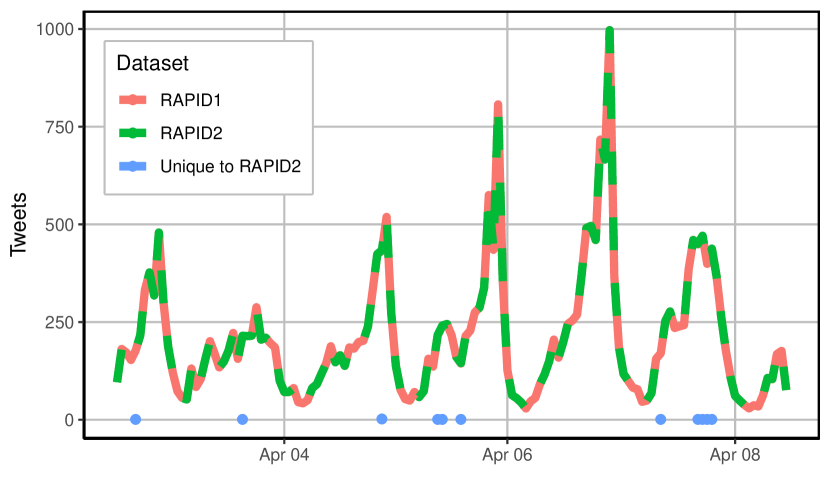
Figure 15: Twitter activity in the AFL2 dataset over time (in 60 minute blocks). Thick and dashed lines are used here to highlight how the timeseries overlap almost exactly. The timestamps of tweets unique to RAPID2 are shown as blue points.

Given it appeared that different collection tools could produce different results using the same inputs, the question of whether APIs are delivering consistent content for all clients remained. A second collection (“AFL2” in Table 4) was initiated over a longer period (six days) using the same filter term and tool (RAPID), but with different API credentials. One set of credentials belonged to a relatively new and unused account (created in 2018 having posted only 3 tweets) and the other to a well-established account (created in 2009 and having posted 17k tweets). This resulted in two highly similar, but not quite identical, datasets, with sizes $30,103$ and $30,115$ tweets; their timeline is shown in Figure 15. The first dataset was a proper subset of the second, so the difference of $12$ posts can be regarded as due to noise or minor differences in timing. A brief examination revealed these extra tweets (shown in blue in the Figure) were all about AFL or other sports in Australia, and their timing appeared random. Further confirmation of the similarity between datasets can be seen in Table 15 where the most prolific account, most retweeted tweet, most replied to tweet and most mentioned account details are all identical. Again, the most mentioned account is the official @AFL account.

Property	RAPID1	RAPID2
Tweet count	30,103	30,115
Retweet count	9,215	9,215
Account count	14,231	14,232
Quote count	2,340	2,341
Reply count	9,229	9,229
Tweets with hashtags	8,623	8,627
Tweets with URLs	11,467	11,474
Most prolific account	Account $a_{7}$	Account $a_{7}$
Most prolific account tweet count	612	612
Most retweeted tweet	Tweet $t_{7}$	Tweet $t_{7}$
Most retweeted tweet count	269	269
Most replied to tweet	Tweet $t_{8}$	Tweet $t_{8}$
Most replied to tweet count	206	206
Tweets with mentions	22,083	22,083
Most mentioned account	Account $a_{6}$	Account $a_{6}$
Most mentioned account count	10,468	10,468
Hashtag uses	20,136	20,140
Unique hashtags	3,337	3,337
Most used hashtag	#afl	#afl
Most used hashtag count	5,096	5,096
Next most used hashtag	#afldeesdons	#afldeesdons
Uses of next most used hashtag	759	759
URL uses	5,702	5,709
Unique URLs	3,580	3,587
Most used URL	http://watchrugby.net/AFL/	http://watchrugby.net/AFL/
Most used URL count	341	341

Table 15: Statistics of two parallel datasets collected using RAPID with the filter term “afl” over a six day period with different API credentials.

4.3.1 Comparison of network statistics

			MENTION		REPLY
Dataset	Tweets	Accounts	Nodes	Edges	Nodes	Edges
RAPID1	30,103	14,231	15,323	31,859	6,778	7,655
RAPID2	30,115	14,232	15,323	31,859	6,778	7,655

Table 16: Selected comparative statistics for networks generated from the two RAPID datasets for the AFL2 collection.

Due to the similarity of the datasets, the retweet, mention and reply networks generated from them were almost identical, and only a summary of the structures is provided in Table 16. Details of the networks are provided in Figure 16, which show that the only differences occur in the detected clusters. In particular, the largest cluster detected in the RAPID2 mention network is around $3\%$ larger than the corresponding cluster from the RAPID1 mention network. This is likely due to an element of randomness used in the Louvain algorithm (Blondel et al., 2008).

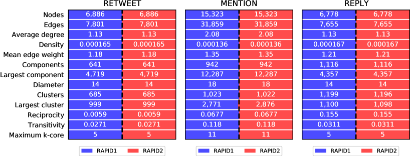
Figure 16: The proportional balance between the RAPID1 and RAPID2 statistics of the retweet, mention and reply networks built from the AFL2 datasets.

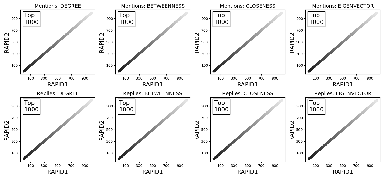
Figure 17: Centrality ranking comparison scatter plots of the mention and reply networks built from the AFL2 datasets. In each plot, each point represents a node’s ranking in the RAPID1 and RAPID2 lists of centralities (common nodes amongst the top $1,000$ of each list). The number of nodes appearing in both lists is inset. Point darkness indicates rank on the $x$ axis (darker = higher).

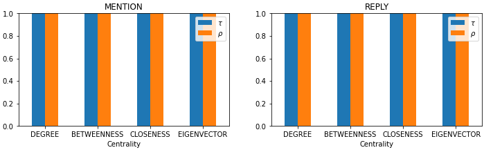
Figure 18: Centrality ranking comparisons from the two RAPID datasets of the AFL2 collection using Kendall Tau scores and Spearman’s Coefficients.

4.3.2 Comparison of centralities and clusters

The similarity of the networks based on their statistics is further confirmed by a comparison of their centrality rankings, which indicates that their structures are all but identical. A visual inspection of their respective rankings in Figure 17 reveals no major differences, and the Kendall Tau and Spearman’s coefficients indicate their rankings are, in fact identical (Figure 18).

RETWEET	MENTION	REPLY
0.916	0.808	0.865

Table 17: Adjusted Rand index scores for the clusters found in the networks built from the RAPID and Twarc datasets for the AFL2 collection.

Interestingly, the high degree of similarity does not extend to the membership of detected clusters using the ARI measure (Table 17). Presumably, the sensitivity of the measure indicates that these scores must be as close to the maximum as we could expect due to the degree of randomness inherent in Louvain clustering. For a score of $1.0$ each pair of detected clusters would need to match perfectly, across the thousands of nodes in the networks, so any minor variation will reduce that score.

4.3.3 Summary of findings

This evidence suggests that the results provided by the Twitter API (if not other platforms’ APIs) are consistent, regardless of the consumer. It is clearly important that a researcher understand how their collection tool works to guarantee their understanding of the results returned. In this regard, open source solutions are, as the name implies, more transparent than closed source solutions. The benefit gained as a result of more tailored filtering must be balanced against the initial effort required to understand how the APIs are employed by the tool used and what modifications tools make to the data they collect.

4.4 Case Study 4: Election Day

A final case study highlights the importance of continuous network connectivity, and awareness of when that condition is not met. To consider a more focused collection activity and to consider a second open source collection tool (thus similar to the baseline tool, Twarc), a collection was conducted over an election day (24 hour period) in early 2019, using RAPID, Twarc and Tweepy, each configured with the same filter terms: #nswvotes, #nswelection, #nswpol, and #nswvotes2019. RAPID and Twarc collected slightly below 40k tweets each while Tweepy collected around 36k tweets, but suffered from network outages on two occasions for approximately $110$ and $96$ minutes each time (see Figure 19). In the resulting datasets (highlights of which are shown in Table 18), $285$ tweets were unique to RAPID, three to Twarc, and $19$ were shared by Twarc and Tweepy but not RAPID. The vast majority of the Tweepy dataset’s $36,172$ tweets appeared in all three datasets, while Tweepy missed the $3,118$ further tweets that appeared in both Twarc and RAPID datasets. In fact, by examining the periods where Tweepy lost its connection, around 6 p.m. (UTC) and again approximately six hours later, Twarc retained $3,036$ tweets while RAPID retained $3,055$ tweets (RAPID-E collected $3,918$ during these periods), so it is possible that if Tweepy’s connection had stayed up, the Tweepy dataset might have been very similar to Twarc and RAPID, especially as the remainder of the collection behaviour of the tools appears almost identical in the timeline.

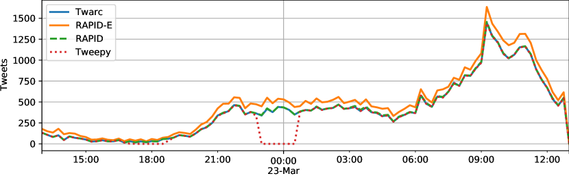
Figure 19: Twitter activity in the Election Day dataset over time (in 15 minute blocks). Dashed and dotted lines are used here to highlight how the timeseries overlap almost exactly.

Dataset	All	Unique		Retweets		All	Unique
	Tweets	Tweets				Accounts	Accounts
Twarc	39,293	3	(0.0%)	26,412	(67.2%)	10,860	1	(0.0%)
RAPID	39,556	285	(0.7%)	26,612	(67.3%)	10,893	36	(0.3%)
RAPID-E	46,526	7,255	(15.6%)	30,735	(66.1%)	12,696	1,839	(14.5%)
Tweepy	36,172	0	(0.0%)	24,276	(67.1%)	10,242	0	(0.0%)

Table 18: Summary dataset statistics of the Election Day collection.

4.4.1 Comparison of collection statistics

The collection statistics are highly similar and are provided primarily for completeness. The effect of Tweepy’s disconnection is highlighted by the differences in its statistics from Twarc as the baseline. Although more than $3,000$ tweets were missed, only a few hundred accounts, quotes, replies and tweets with URLs were missed. Several thousand retweets were missed as well as tweets with hashtags and mentions, but the effect on the features with the highest counts is limited. The most prolific account, most retweeted tweet, most replied to tweet, most mentioned accounts, hashtags and URLs are all the same.

Property	Twarc	RAPID	Tweepy
Tweets	39,297	39,556	36,172
Accounts	10,860	10,893	10,242
Retweets	26,412	26,612	24,276
Quotes	3,590	3,610	3,363
Replies	1,374	1,381	1,252
Tweets with hashtags	21,582	21,686	19,977
Tweets with URLs	7,829	7,860	7,194
Most prolific account	Account $a_{8}$	Account $a_{8}$	Account $a_{8}$
Tweets by most prolific account	212	211	212
Most retweeted tweet	Tweet $t_{9}$	Tweet $t_{9}$	Tweet $t_{9}$
Most retweeted tweet count	368	367	278
Most replied to tweet	Tweet $t_{10}$	Tweet $t_{10}$	Tweet $t_{10}$
Most replied to tweet count	25	26	24
Tweets with mentions	30,626	30,848	28,154
Most mentioned account	Account $a_{9}$	Account $a_{9}$	Account $a_{9}$
Mentions of most mentioned account	2,442	2,443	2,187
Hashtag uses	51,288	51,470	47,106
Unique hashtags	2,450	2,458	2,306
Most used hashtag	#nswvotes	#nswvotes	#nswvotes
Most used hashtag count	11,739	11,731	10,901
Next most used hashtag	#nswvotes2019	#nswvotes2019	#nswvotes2019
Uses of next most used hashtag	7,606	7,602	6,968
URL uses	3,766	3,761	3,478
Unique URLs	1,374	1,374	1,258
Most used URL	URL 1*	URL 1*	URL 1*
Uses of most used URL	100	100	100

Table 19: Statistics of the Twarc, RAPID, and Tweepy datasets collected in parallel over a $24$ hour period. ^*https://www.fiverr.com/s2/ee030ef08d

4.4.2 Comparison of network statistics

Continuing the similarities in the collection statistics, statistics drawn from retweet, mention and reply networks built from the Election Day datasets are also strikingly resilient, despite the Tweepy networks including several hundred fewer nodes (Table 20). This is borne out by the proportional differences between Twarc and RAPID in Figure 20, where the only significant difference is the size of the largest detected cluster (again, likely due to the randomness inherent in Louvain (Blondel et al., 2008)), and then in the proportional differences in all the statistics across the Twarc and Tweepy networks in Figure 21.

	RETWEET			MENTION			REPLY
	Twarc	RAPID	Tweepy	Twarc	RAPID	Tweepy	Twarc	RAPID	Tweepy
Number of nodes	8,620	8,649	8,193	10,117	10,161	9,600	1,234	1,238	1,147
Number of edges	22,895	23,056	21,122	36,360	36,589	33,595	1,174	1,181	1074
Average degree	2.656	2.666	2.578	3.594	3.601	3.500	0.951	0.954	0.936
Density	0.000	0.000	0.000	0.000	0.000	0.000	0.001	0.001	0.001
Mean edge weight	1.154	1.154	1.149	1.217	1.218	1.209	1.170	1.169	1.166
Component count	183	183	183	183	183	178	298	297	286
Largest component	8,199	8,228	7,779	9,687	9,731	9,146	642	648	569
- Diameter	13	13	13	12	12	12	18	18	19
Clusters	207	210	210	209	209	204	319	316	304
Largest cluster	1,243	1,503	1,405	1,507	1,585	1,582	54	53	53
Reciprocity	0.009	0.009	0.009	0.020	0.020	0.019	0.012	0.012	0.011
Transitivity	0.035	0.035	0.032	0.060	0.060	0.058	0.001	0.001	0.001
Maximum k-core	15	15	14	20	20	19	2	2	2

Table 20: Comparative statistics for networks generated from the Twarc, RAPID and Tweepy datasets for the Election Day collection.

Figure 20: The proportional balance between Twarc and RAPID statistics of the retweet, mention and reply networks built from the Twarc and RAPID datasets.

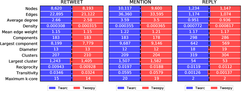
Figure 21: The proportional balance between Twarc and RAPID statistics of the retweet, mention and reply networks built from the Twarc and Tweepy datasets.

4.4.3 Comparison of centralities

Examining the centralities of the mention and reply networks built from the Election Day datasets, comparing RAPID and Tweepy against the Twarc baseline shows, as expected, only minor variations in the RAPID dataset which only occur among the lower ranked nodes (Figure 22) and more widespread differences with the Tweepy networks (Figure 23). Statistically, Twarc and RAPID’s mention network centrality rankings, shown in Figure 24, had Kendall $\tau$ values around $0.35$ to $0.4$ and Spearman’s coefficients around $0.45$ to $0.6$, while the reply networks’ values were higher, with $\tau$ around $0.5$ and Spearman’s coefficient around $0.7$, possibly due to the smaller size of the reply networks. These values are all approaching or exceeding the $\tau$ value of $0.4$ to $0.6$ that was regarded as reasonably to highly similar, mentioned in Section 3.4. The ranking similarity statistics calculated by comparing the Twarc and Tweepy baselines are notably lower (Figure 25, though even the reply networks’ betweenness and closeness comparisons are moderately similar with $\tau$ around $0.4$ and Spearman’s coefficient around $0.5$ to $0.6$.

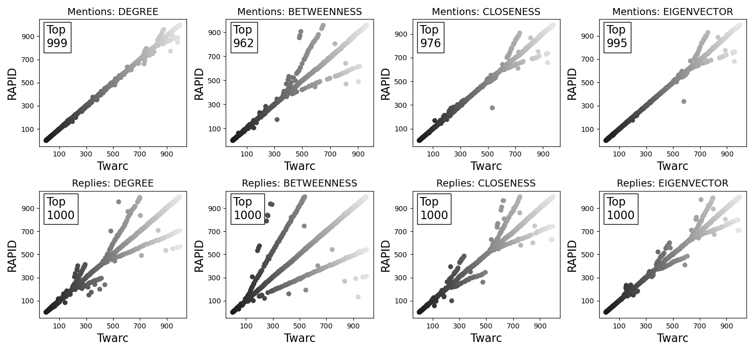
Figure 22: Centrality ranking comparison scatter plots of the mention and reply networks built from the Twarc and RAPID Election Day datasets. In each plot, each point represents a node’s ranking in the RAPID1 and RAPID2 lists of centralities (common nodes amongst the top $1,000$ of each list). The number of nodes appearing in both lists is inset. Point darkness indicates rank on the $x$ axis (darker = higher).

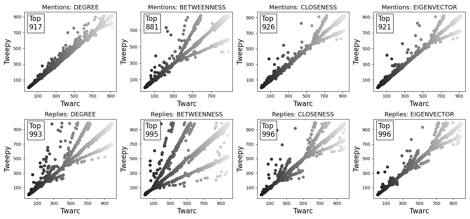
Figure 23: Centrality ranking comparison scatter plots of the mention and reply networks built from the Twarc and Tweepy Election Day datasets. In each plot, each point represents a node’s ranking in the RAPID1 and RAPID2 lists of centralities (common nodes amongst the top $1,000$ of each list). The number of nodes appearing in both lists is inset. Point darkness indicates rank on the $x$ axis (darker = higher).

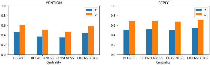
Figure 24: Centrality ranking comparisons from the Twarc and RAPID datasets of the Election Day collection using Kendall Tau scores and Spearman’s Coefficients.

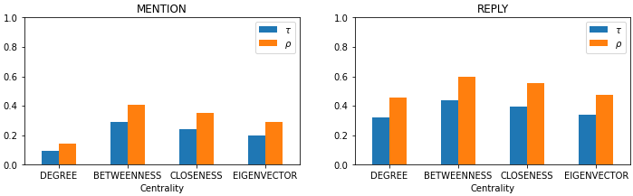
Figure 25: Centrality ranking comparisons from the Twarc and Tweepy datasets of the Election Day collection using Kendall Tau scores and Spearman’s Coefficients.

4.4.4 Comparison of clusters

Despite the similarities between the Twarc and RAPID networks, the cluster membership still varies significantly, with the highest similarity being found amongst the (smaller) reply networks, as can be seen in the ARI scores in Table 21. The clusters found in the Twarc and Tweepy networks are less similar, almost in line with the differences in network sizes: the retweet networks had fewer nodes than the mention networks, and the ARI scores are less different, and the reply networks were the smallest and had the smallest difference between ARI scores.

	RETWEET	MENTION	REPLY
Twarc/RAPID	0.547	0.656	0.737
Twarc/Tweepy	0.453	0.534	0.703

Table 21: Adjusted Rand index scores for the clusters found in the corresponding retweet, mention and reply networks built from the Election Day datasets.

4.4.5 Summary of findings

This final case study provides us with further confidence that the differences observed early on in the Q&A datasets are primarily caused by enhancements provided by the RAPID platform and the differences in the AFL1 datasets were due, in part, to the choice of “afl” as the lone filter term. The Election Day collection used several specific filter terms and ran long enough to collect several tens of thousands of tweets, enough time to avoid minor differences in start and stop times. Even the differences that did occur did not result in significant effects on several networks constructed from the data or on network analysis measures calculated over those networks.

5 Discussion

The case studies presented highlight how decisions regarding collection specification, such as the filter terms used or their number, and the collection duration, can result in datasets that trigger features in complex collection tools, quite apart from configuration of such tools to dynamically change the collection specification (e.g., use of RAPID’s topic tracking feature). The primary variations explored here involved filter terms although collection duration also varied, depending on the collection event. The biggest variations in parallel datasets appeared when few filter terms were used and when they were short (i.e., having few characters), resulting in incidental noise from posts in unexpected languages (#qanda) or with unexpected acronyms and from elements in post metadata (#afl). When multiple terms were used, and when those terms were not valid words in a language (e.g., variations on #nswelec), the parallel datasets were much more similar. Although it might be common sense to encourage careful design of collection specifications, these case studies highlight the value in (and danger in not) being more specific, by dictating the language of posts required as well as using multiple filter terms.

When variations in datasets occurred, the extra tweets resulted in the introduction of new nodes (accounts) in retweet, mention and reply networks, the majority of which were located within the largest connected network components (relatively few appeared as new, independent components). This consistently reduced the density of the retweet, mention and reply networks, but rarely affected the diameter of the largest component (Q&A Part 2’s retweet network is an exception here), implying that the new nodes appear in the core of the components, rather than on the periphery. Consequently, the extra nodes increased reciprocity, transitivity, and sometimes maximum k-core values in retweet and mention networks, but rarely changed reply networks. Reply interactions occurred least frequently in all datasets, and so reply networks were the least different in raw size (nodes and edges).

The effects of collection variation were most prominent in centrality scores, particularly when the collection event involved direct interaction between participants (e.g., issue- or theme-based discussions such as during Q&A and over weekends of football) and less straightforward information dissemination (e.g., during an election campaign). The ranking of nodes by centrality varied most in the mention and reply networks of Q&A Part 1, even though more than half the top thousand ranked nodes in each pair of parallel networks were the same (an average of $560.5$ for mentions and $991$ for replies). The forking patterns appearing in scatter plots imply the presence of groups of nodes with adjacent centrality rankings, which then swapped when new nodes were added, possibly through impacting the internal topology of the largest components in some way. Spearman’s $\rho$ and Kendall $\tau$ correlation coefficients were consistently higher for reply networks than mention networks, possibly due to their smaller size. No particular patterns in differences between centrality types were observed, which implies the differences between pairs of parallel networks did not result in significantly different topologies.

A final lesson drawn from the use of ARI scores is that even clustering of highly similar (e.g., almost identical) networks (in Case Study $4$), result in ARI scores around $0.7$, meaning that ARI scores around $0.4$ can be seen as confirmation cluster membership is, in fact, quite similar.

The central purpose of this paper is to draw attention to unexpected variations in datasets collected from social media streams and the networks constructed from them. This is especially relevant when it is known that the stream is limited (either through platform rate-limiting or through platform algorithms, as occurs with, say, Twitter’s 1% sample stream). An obvious follow-up question is whether or not an objective measure of reliability is feasible. This relates closely to the question of how representative samples provided by platforms are of their entire data holdings, e.g., as studied by  Morstatter et al. (2013); González-Bailón et al. (2014); Joseph et al. (2014), but that question relies on examining the choices made by the platform in deciding what to include in the sample they offer. Here, similar to Paik & Lin Paik and Lin (2015), our interest is in confirming that the data we request from a platform (with filter terms) matches what it has, or is at least representative of what it has (if rate-limits are encountered). Such a measure might rely on comparing the distributions of various features in our result dataset and the overall dataset (held by the platform), such as the accounts and the number of tweets they post, the number of hashtags, URLs, and mentioned used and replies, quotes and retweets made. Only the platform has sufficient information to provide this measure, and there may be significant value in them doing it for free or low cost streams they provide to researchers, analysts and other social media mass consumers. Providing a measure of representativeness (indicating reliability) along with results could: 1) encourage consumers to pay for the higher cost streams, while also 2) providing consumers with more certainty in any conclusions they draw from the results they analyse. A measure of reliability rather than representativeness could be more useful also, because there may be good reason for the results of filters that the platform provides to not be truly representative – this would be the case when the full dataset includes significant amounts of spam or pornography. The reliability measure would indicate how representative the provided results are compared with the full results.

6 Conclusion

Under a variety of conditions, the collection tools employed in several use cases provided different views of specific online discussions. These differences manifested as variations in collection statistics, and network-level and node-level statistics for retweet, mention and reply social networks built from the collected data. Extra tweets were most often collected by Twarc, and these appear to have resulted in more connections in the largest components without affecting their diameters. This may affect results of diffusion analysis, as reachability correspondingly increases. Deeper study of reply content is required to inform discussion patterns.

How reliable social media can be as a source for research without deep knowledge of the effects of collection tools on analyses is an open question. If a tool adds value through analytics, what is the nature of the effect? This paper provides a methodology to explore those effects. A canonical measure of the reliability of a dataset would be valuable to the research and broader social media analysis community. This measure would explain how complete the results of a search or filter of live posts is, and if it is not complete, how representative the provided sample results are of the complete results. Only the platforms have this information to hand, however there would be benefits for them to do so, including as an enticement to consumers to pay for greater access to platform data holdings, as well as helping inform consumers of the degree to which they can depend on analyses of the data they receive.

We recommend the following to those using OSN data:

• Be aware of tool biases and their effects.

• Take care to specify filter and search conditions with keywords that capture relevant data and avoid irrelevant data, and make use of metadata filters to avoid unwanted content, e.g., constraining language code. Beware of short filter terms and ones that are meaningful in non-target languages.

• Check the integrity of data. We observed gaps and minor inconsistencies in the Election case study due to connection failures as well as the appearance of duplicate tweets, identical in data and metadata.

There are a number of avenues by which to expand this research:

• Consolidate and expand the methodology so that it may be applied to other OSNs and collection tools, especially proprietary ones. A method to shed light on the biases of tools would be of great value to the community.

• Introduce content analysis to the comparison. If social networks built from parallel datasets vary, what is the effect on analyses of the discussion? Are text analysis methods robust enough to overcome differences or is it possible to draw entirely different conclusions, depending on the method used?

• Examine differences in information flow based on clusters rather than just individual nodes to help inform questions about broad information flow within the networks. If the differences are moderate, then we may draw confidence that overall flows of influence in a network may remain relatively steady, even with variations in the collection.

• Although OSNs are similar when the interaction primitives they offer are considered, the way in which their feature sets are presented in user interfaces create a platform-specific interaction culture, and that affects the observable behaviour of its users, which may in turn affect analyses. An exploration of how platform culture manifests itself and differs would help inform the search for higher level social activities such as coordination (Grimme et al., 2018; Pacheco et al., 2020; Weber and Neumann, 2020; Graham et al., 2020).

• Key for future social media research is to develop processes for repeatable analysis, including access to common datasets, both of which underpin the practice of benchmarking. Currently, OSN terms and conditions often hamper researchers exchanging datasets, so new techniques cannot easily be evaluated on the same data, raising questions of fair comparison. For example, Twitter requires that only tweet IDs are shared, forcing the next researcher to ‘re-hydrate’ the tweets by downloading them again from Twitter’s servers. By the time a new researcher does this, the data may have changed: metadata, such as retweet and like counts are constantly incremented; tweets and entire accounts may have been deleted or removed through suspension or account closure; or accounts may become private and inaccessible.

Finally: Does it matter if a streamed collection is not necessarily either complete or representative? As long as a researcher makes clear how they conducted a collection and using what tools and configuration, does it not still result in an analysis of behaviour that occurred online? The answer is that it very much depends on the conclusions being drawn. Yes, the collection represents real activity that occurred, but it may not be complete, and conclusions drawn from it may be unintentionally misinformed and lacking in nuance. We have seen that variations in collections have an impact on network size and structure. This may result in different community compositions and affect centrality analyses, consequently misleading influential account identification and expected diffusion patterns. A firm understanding of the data and how it was obtained is therefore vital.

Declarations

Funding

Mehwish Nasim acknowledges that this work has been partially supported by the Cyber Security Research Centre Limited whose activities are partially funded by the Australian Government’s Cooperative Research Centres Programme.

Conflicts of interest/Competing interests

Not applicable.

Availability of data and material

The data (the identifiers of tweets only, as per Twitter’s terms and conditions) used in this study are available at https://github.com/weberdc/socmed_sna.

Code availability

The data manipulation and analysis software written for this study is available at https://github.com/weberdc/socmed_sna.

Authors’ contributions

All authors contributed to the study conception and design. Data collection was performed by Derek Weber, Lewis Mitchell, and Mehwish Nasim, and analysis was performed by Derek Weber, while advised by Mehwish Nasim, Lewis Mitchell and Lucia Falzon. The first draft of the manuscript was written primarily by Derek Weber with contributions from the other authors, and all authors commented on previous versions of the manuscript. All authors read, edited and approved the final manuscript.

Ethics approval

All data were collected, stored, processed and analysed according to two ethics protocols #170316 and H-2018-045, approved by the University of Adelaide’s human research and ethics committee.

Consent to participate

Not applicable.

Consent for publication

All authors consent to this work being published.

References

- Bagrow et al. (2019) Bagrow JP, Liu X, Mitchell L (2019) Information flow reveals prediction limits in online social activity. Nature Human Behaviour 3(2):122–128, DOI 10.1038/s41562-018-0510-5
- Bessi and Ferrara (2016) Bessi A, Ferrara E (2016) Social bots distort the 2016 U.S. Presidential election online discussion. First Monday 21(11), URL http://firstmonday.org/ojs/index.php/fm/article/view/7090
- Blondel et al. (2008) Blondel VD, Guillaume JL, Lambiotte R, Lefebvre E (2008) Fast unfolding of communities in large networks. Journal of Statistical Mechanics: Theory and Experiment 2008(10):P10008, DOI 10.1088/1742-5468/2008/10/p10008
- Borgatti et al. (2009) Borgatti SP, Mehra A, Brass DJ, Labianca G (2009) Network analysis in the social sciences. Science 323(5916):892–895, DOI 10.1126/science.1165821
- Borgatti et al. (2013) Borgatti SP, Everett MG, Johnson JC (2013) Analyzing social networks, 1st edn. SAGE, Los Angeles
- Brin and Page (1998) Brin S, Page L (1998) The anatomy of a large-scale hypertextual web search engine. Computer networks and ISDN systems 30(1-7):107–117
- Cao et al. (2015) Cao C, Caverlee J, Lee K, Ge H, Chung J (2015) Organic or organized?: Exploring URL sharing behavior. In: CIKM, ACM, pp 513–522
- Cresci et al. (2017) Cresci S, Pietro RD, Petrocchi M, Spognardi A, Tesconi M (2017) The paradigm-shift of social spambots: Evidence, theories, and tools for the arms race. In: WWW (Companion Volume), ACM, pp 963–972
- Dancey and Reidy (2011) Dancey C, Reidy J (2011) Statistics without maths for psychology, 5th edn. Prentice Hall/Pearson, Harlow, England New York
- Davis et al. (2016) Davis CA, Varol O, Ferrara E, Flammini A, Menczer F (2016) BotOrNot: A system to evaluate social bots. In: WWW (Companion Volume), ACM, pp 273–274
- Edwards et al. (2018) Edwards M, Mitchell L, Tuke J, Roughan M (2018) The one comparing narrative social network extraction techniques. arXiv preprint arXiv:181101467
- Falzon et al. (2017) Falzon L, McCurrie C, Dunn J (2017) Representation and analysis of Twitter activity: A dynamic network perspective. In: ASONAM, ACM, pp 1183–1190
- Falzon et al. (2018) Falzon L, Quintane E, Dunn J, Robins G (2018) Embedding time in positions: Temporal measures of centrality for social network analysis. Social Networks 54:168–178
- Ferrara (2017) Ferrara E (2017) Disinformation and social bot operations in the run up to the 2017 French presidential election. First Monday 22(8)
- Ferrara et al. (2016) Ferrara E, Varol O, Davis CA, Menczer F, Flammini A (2016) The rise of social bots. Communications of the ACM 59(7):96–104
- Giglietto et al. (2020) Giglietto F, Righetti N, Rossi L, Marino G (2020) It takes a village to manipulate the media: Coordinated link sharing behavior during 2018 and 2019 Italian elections. Information, Communication & Society pp 1–25, DOI 10.1080/1369118x.2020.1739732
- González-Bailón et al. (2014) González-Bailón S, Wang N, Rivero A, Borge-Holthoefer J, Moreno Y (2014) Assessing the bias in samples of large online networks. Social Networks 38:16–27
- Goodman (1961) Goodman LA (1961) Snowball sampling. The Annals of Mathematical Statistics 32(1):148–170, DOI 10.1214/aoms/1177705148
- Graham et al. (2020) Graham T, Bruns A, Angus D, Hurcombe E, Hames S (2020) #IStandWithDan versus #DictatorDan: the polarised dynamics of Twitter discussions about Victoria’s COVID-19 restrictions. Media International Australia p 1329878X2098178, DOI 10.1177/1329878x20981780
- Gray et al. (2020) Gray C, Mitchell L, Roughan M (2020) Bayesian inference of network structure from information cascades. IEEE Transactions on Signal and Information Processing over Networks 6:371–381
- Grimme et al. (2018) Grimme C, Assenmacher D, Adam L (2018) Changing perspectives: Is it sufficient to detect social bots? In: Meiselwitz G (ed) Social Computing and Social Media. User Experience and Behavior, Springer International Publishing, Cham, pp 445–461
- Gruzd (2011) Gruzd A (2011) Imagining Twitter as an imagined community. American Behavioral Scientist 55(10):1294–1318
- Holzmann et al. (2018) Holzmann H, Anand A, Khosla M (2018) Delusive PageRank in incomplete graphs. In: COMPLEX NETWORKS (1), Springer, Studies in Computational Intelligence, vol 812, pp 104–117
- Hubert and Arabie (1985) Hubert L, Arabie P (1985) Comparing partitions. Journal of Classification 2(1):193–218, DOI 10.1007/BF01908075
- Joseph et al. (2014) Joseph K, Landwehr PM, Carley KM (2014) Two 1%s don’t make a whole: Comparing simultaneous samples from Twitter’s streaming API. In: Kennedy WG, Agarwal N, Yang SJ (eds) Social Computing, Behavioral-Cultural Modeling and Prediction, Springer International Publishing, Cham, pp 75–83
- Keller et al. (2017) Keller F, Schoch D, Stier S, Yang J (2017) How to manipulate social media: Analyzing political astroturfing using ground truth data from South Korea. In: ICWSM, AAAI Press, pp 564–567
- Lazer et al. (2014) Lazer D, Kennedy R, King G, Vespignani A (2014) The Parable of Google Flu: Traps in Big Data Analysis. Science (New York, NY) 343:1203–5, DOI 10.1126/science.1248506
- Lim et al. (2018) Lim K, Jayasekara S, Karunasekera S, Harwood A, Falzon L, Dunn J, Burgess G (2018) RAPID: Real-time Analytics Platform for Interactive Data Mining. In: ECML/PKDD (3), Springer, LNCS, vol 11053, pp 649–653
- Morstatter et al. (2013) Morstatter F, Pfeffer J, Liu H, Carley KM (2013) Is the sample good enough? comparing data from Twitter’s streaming API with Twitter’s firehose. In: ICWSM, AAAI Press, pp 400–408
- Morstatter et al. (2018) Morstatter F, Shao Y, Galstyan A, Karunasekera S (2018) From Alt-Right to Alt-Rechts: Twitter analysis of the 2017 German Federal Election. In: WWW (Companion Volume), ACM, pp 621–628
- Nasim (2016) Nasim M (2016) Inferring social relations from online and communication networks. PhD thesis, Computer and Information Science
- Nasim et al. (2018) Nasim M, Nguyen A, Lothian N, Cope R, Mitchell L (2018) Real-time detection of content polluters in partially observable Twitter networks. In: WWW (Companion Volume), ACM, pp 1331–1339
- Newman (2010) Newman MEJ (2010) Networks : An Introduction. Oxford University Press
- Nizzoli et al. (2020) Nizzoli L, Tardelli S, Avvenuti M, Cresci S, Tesconi M (2020) Coordinated behavior on social media in 2019 UK general election. CoRR abs/2008.08370, 2008.08370v1
- Olteanu et al. (2019) Olteanu A, Castillo C, Diaz F, Kıcıman E (2019) Social data: Biases, methodological pitfalls, and ethical boundaries. Frontiers in Big Data 2:13, DOI 10.3389/fdata.2019.00013
- Pacheco et al. (2020) Pacheco D, Flammini A, Menczer F (2020) Unveiling coordinated groups behind White Helmets disinformation. In: WWW (Companion Volume), ACM / IW3C2, pp 611–616
- Paik and Lin (2015) Paik JH, Lin J (2015) Do multiple listeners to the public Twitter sample stream receive the same tweets? In: TAIA
- Pfeffer et al. (2018) Pfeffer J, Mayer K, Morstatter F (2018) Tampering with Twitter’s sample API. EPJ Data Science 7(1):50
- Ratkiewicz et al. (2011) Ratkiewicz J, Conover M, Meiss M, Gonçalves B, Flammini A, Menczer F (2011) Detecting and tracking political abuse in social media. In: ICWSM, AAAI Press, pp 297–304
- Rizoiu et al. (2018) Rizoiu MA, Graham T, Zhang R, Zhang Y, Ackland R, Xie L (2018) #DebateNight: The role and influence of socialbots on Twitter during the 1st 2016 U.S. Presidential debate. In: ICWSM, AAAI Press, pp 300–309
- Robins (2015) Robins G (2015) Doing social network research: network-based research design for social scientists. Sage
- Ruths and Pfeffer (2014) Ruths D, Pfeffer J (2014) Social media for large studies of behavior. Science 346(6213):1063–1064, DOI 10.1126/science.346.6213.1063
-
Scott (2021)
Scott M (2021) Capitol Hill riot lays bare what’s wrong with social media.
https://www.politico.eu/article/us-capitol-hill-riots-lay-bare-whats-wrong
-social-media-donald-trump-facebook-twitter/, last accessed on 8 February 2021. - Tromble et al. (2017) Tromble R, Storz A, Stockmann D (2017) We don’t know what we don’t know: When and how the use of Twitter’s public APIs biases scientific inference. In: SSRN, pp 1–26
- Tufekci (2014) Tufekci Z (2014) Big questions for social media Big Data: Representativeness, validity and other methodological pitfalls. In: ICWSM, The AAAI Press, pp 505–514
- Tuke et al. (2020) Tuke J, Nguyen A, Nasim M, Mellor D, Wickramasinghe A, Bean N, Mitchell L (2020) Pachinko prediction: A bayesian method for event prediction from social media data. Information Processing & Management 57(2):102147
- Venturini et al. (2018) Venturini T, Munk A, Jacomy M (2018) Actor-network vs network analysis vs digital networks are we talking about the same networks? In: Ribes V, Vertesi J (eds) Digital STS: A Handbook and Fieldguide, Palgrave Macmillan, New York, pp 510–524
- Vo et al. (2017) Vo N, Lee K, Cao C, Tran T, Choi H (2017) Revealing and detecting malicious retweeter groups. In: ASONAM, ACM, pp 363–368
- Wasserman and Faust (1994) Wasserman S, Faust K (1994) Social network analysis: Methods and applications, vol 8. Cambridge University Press
- Weber and Neumann (2020) Weber D, Neumann F (2020) Who’s in the gang? Revealing coordinating communities in social media. In: ASONAM, ACM
- Weber et al. (2020a) Weber D, Nasim M, Falzon L, Mitchell L (2020a) #ArsonEmergency and Australia’s “Black Summer”: Polarisation and misinformation on social media. In: MISDOOM, Springer, Lecture Notes in Computer Science, vol 12259, pp 159–173
- Weber et al. (2020b) Weber D, Nasim M, Mitchell L, Falzon L (2020b) A method to evaluate the reliability of social media data for social network analysis. In: ASONAM, ACM
- Woolley and Howard (2018) Woolley S, Howard P (eds) (2018) Computational Propaganda: Political Parties, Politicians, and Political Manipulation on Social Media, Oxford University Press, chap 8, pp 185–211. Oxford Studies in Digital Politics, DOI 10.1093/oso/9780190931407.001.0001
- Woolley (2016) Woolley SC (2016) Automating power: Social bot interference in global politics. First Monday 21(4), DOI 10.5210/fm.v21i4.6161
- Wu et al. (2016) Wu L, Morstatter F, Hu X, Liu H (2016) Mining misinformation in social media. Big data in complex and social networks pp 123–152
- Wu et al. (2018) Wu T, Wen S, Xiang Y, Zhou W (2018) Twitter spam detection: Survey of new approaches and comparative study. Computers & Security 76:265–284, DOI 10.1016/j.cose.2017.11.013
- Yang et al. (2016) Yang Z, Algesheimer R, Tessone CJ (2016) A comparative analysis of community detection algorithms on artificial networks. Scientific Reports 6(30750):1–16, DOI 10.1038/srep30750
- Yap (2020) Yap AJ (2020) Coronavirus: Why people are panic buying loo rolls and how to stop it. https://theconversation.com/coronavirus-why-people-are-panic-buying-loo-roll-and-how-to-stop-it-133115, last accessed on 10 March 2020.