Measuring Model Biases in the Absence of Ground Truth

Abstract.

The measurement of bias in machine learning often focuses on model performance across identity subgroups (such as $man$ and $woman$) with respect to groundtruth labels (Hardt et al., 2016). However, these methods do not directly measure the associations that a model may have learned, for example between labels and identity subgroups. Further, measuring a model’s bias requires a fully annotated evaluation dataset which may not be easily available in practice.

We present an elegant mathematical solution that tackles both issues simultaneously, using image classification as a working example. By treating a classification model’s predictions for a given image as a set of labels analogous to a “bag of words” (Jurafsky and Martin, 2009), we rank the biases that a model has learned with respect to different identity labels. We use $\{man,woman\}$ as a concrete example of an identity label set (although this set need not be binary), and present rankings for the labels that are most biased towards one identity or the other. We demonstrate how the statistical properties of different association metrics can lead to different rankings of the most “gender biased” labels, and conclude that normalized pointwise mutual information ($nPMI$) is most useful in practice. Finally, we announce an open-sourced $nPMI$ visualization tool using TensorBoard.

1. Introduction

The impact of algorithmic bias in computer vision models has been well-documented (c.f., Buolamwini and Gebru, 2018; Snow, 2018). Examples of the negative fairness impacts of machine learning models include decreased pedestrian detection accuracy on darker skin tones (Wilson et al., 2019), gender stereotyping in image captioning (Burns et al., 2018), and perceived racial identities impacting unrelated labels (Stock and Cisse, 2018). Many of these examples are directly related to currently deployed technology, which highlights the urgency of solving these fairness problems as adoption of these technologies continues to grow.

Many common metrics for quantifying fairness in machine learning models, such as Statistical Parity (Dwork et al., 2011), Equality of Opportunity (Hardt et al., 2016) and Predictive Parity (Chouldechova, 2016), rely on datasets with a significant amount of ground truth annotations for each label under analysis. However, some of the most commonly used datasets in computer vision have relatively sparse ground truth (Kuznetsova et al., 2018). One reason for this is the significant growth in the number of predicted labels. The benchmark challenge dataset PASCAL VOC introduced in 2008 had only 20 categories (Everingham et al., 2015), while less than 10 years later, the benchmark challenge dataset ImageNet provided hundreds of categories (Russakovsky et al., 2015). As systems have rapidly improved, it is now common to use the full set of ImageNet categories, which number more than 20,000 (Deng et al., 2009; Stanford Vision Lab, 2020).

While large label spaces offer a more fine-grained ontology of the visual world, they also increase the cost of implementing groundtruth-dependent fairness metrics. This concern is compounded by the common practice of collecting training datasets from multiple online resources (Lin et al., 2014). This can lead to patterns where specific labels are omitted in a biased way, either through human bias (e.g., crowdsourcing where certain valid labels or tags are omitted systematically) or through algorithmic bias (e.g., selecting labels for human verification based on the predictions of another model (Kuznetsova et al., 2018)). If the ground truth annotations in a sparsely labelled dataset are potentially biased, then the premise of a fairness metric that “normalizes” model prediction patterns to groundtruth patterns may be incomplete. In light of this difficulty, we argue that it is important to develop bias metrics that do not explicitly rely on “unbiased” ground truth labels.

In this work, we introduce a novel approach for measuring problematic model biases, focusing on the associations between model predictions directly. This has several advantages compared to common fairness approaches in the context of large label spaces, making it possible to identify biases after the regular practice of running model inference over a dataset. We study several different metrics that measure associations between labels, building upon work in Natural Language Processing (Church and Hanks, 1990) and information theory. We perform experiments on these association metrics using the Open Images Dataset (Kuznetsova et al., 2018) which has a large enough label space to illustrate how this framework can be generally applied, but we note that the focus of this paper is on introducing the relevant techniques and do not require any specific dataset. We demonstrate that normalized pointwise mutual information ($nPMI$) is particularly useful for detecting the associations between model predictions and sensitive identity labels in this setting, and can uncover stereotype-aligned associations that the model has learned. This metric is particularly promising because:

• It requires no ground truth annotations.

• It provides a method for uncovering biases that the model itself has learned.

• It can be used to provide insight into per-label associations between model predictions and identity attributes.

• Biases for both low- and high-frequency labels are able to be detected and compared.

Finally we announce an open-sourced visualization tool in TensorBoard that allows users to explore patterns of label bias in large datasets using the $nPMI$ metric.

2. Related Work

In 1990, Church and Hanks (Church and Hanks, 1990) introduced a novel approach to quantifying associations between words based on mutual information (Shannon, 1948; Fano, 1961) and inspired by psycholinguistic work on word norms (Toglia and Battig, 1978) that catalogue words that people closely associate. For example, subjects respond more quickly to the word nurse if it follows a highly associated word such as doctor (Greenwald et al., 1998; Caliskan et al., 2017). Church and Hanks’ proposed metric applies mutual information to words using a pointwise approach, measuring co-occurrences of distinct word pairs rather than averaging over all words. This enables a quantification of the question, ”How closely related are these words?” by measuring their co-occurrence rates relative to chance in the dataset of interest. In this case, the dataset of interest is a computer vision evaluation dataset, and the words are the labels that the model predicts.

This information theoretic approach to uncovering word associations became a prominent method in the field of Natural Language Processing, with applications ranging from measuring topic coherence (Aletras and Stevenson, 2013) to collocation extraction (Bouma, 2009) to great effect, although often requiring a good deal of preprocessing in order to incorporate details of a sentence’s syntactic structure. However, without preprocessing, this method functions to simply measure word associations regardless of their order in sentences or relationship to one another, treating words as an unordered set of tokens (a so-called ”bag-of-words”) (Harris, 1954).

As we show, this simple approach can be newly applied to an emergent problem in the machine learning ethics space: The identification of problematic associations that an ML model has learned. This approach is comparable to measuring correlations, although the common correlation metric of Spearman Rank (Spearman, 1904) operates on assumptions that are not suitable for this task, such as linearity and monotonicity. The related correlation metric of the Kendall Rank Correlation (Kendall, 1938) does not require such behavior, and we include comparisons with this approach.

Additionally, many potentially applicable metrics for this problem rely on simple counts of paired words, which does not take into consideration how the words are distributed with other words (e.g., sentence syntax or context); we will elaborate on how this information can be formally incorporated into a bias metric in the Discussion and Future Work sections.

This work is motivated by recent research on fairness in machine learning (e.g., (Hardt et al., 2016)), which at a high level seeks to define criteria that result in equal outcomes across different subpopulations. The focus in this paper is complementary to previous fairness work, honing in on ways to identify and quantify the specific problematic associations that a model may learn rather than providing an overall measurement of a model’s unfairness. It also offers an alternative to fairness metrics that rely on comprehensive ground truth labelling, which is not always available for large datasets.

Open Images Dataset.

The Open Images dataset we use in this work was chosen because it is open-sourced, with millions of diverse images and a large label space of thousands of visual concepts (see (Kuznetsova et al., 2018) for more details). Furthermore, the dataset comes with pre-computed labels generated by a non-trivial algorithm that combines machine-generated predictions and human-verification; this allowed us to focus on analysis of label associations (rather than training a new classifier ourselves) and uncover the most common concepts related to sensitive characteristics, which in this dataset are ${man}$ and ${woman}$.

We now turn to a formal description of the problem we seek to solve.

3. Problem Definition

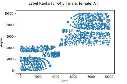
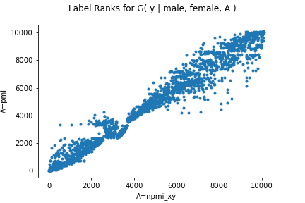
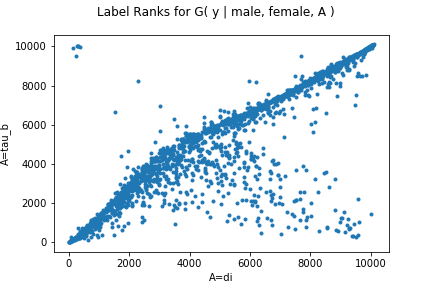
Figure 1. Label ranking shifts for metric-to-metric comparison. Each point represents the rank of a single label when sorted by $G(y|x_{1},x_{2},A(\cdot))$ (i.e., the label rank by gap). The coordinates represent the rankings by gap for different association metrics $A(\cdot)$ on the $x$ and $y$ axes. A highly-correlated plot along $y=x$ would imply that the two metrics lead to very similar bias rankings according to $G(\cdot)$.

We have a dataset $\mathcal{D}$ which contains image examples and labels generated by a image classifier. This classifier takes one image example and predicts “Is label $y_{i}$ relevant to the image?” for each label in $\mathcal{L}=\{y_{1},y_{2},...,y_{n}\}$. We infer $P(y_{i})$ and $P(y_{i},y_{j})$ from $\mathcal{D}$ such that for a given random image in $\mathcal{D}$, $P(y_{i})$ is the probability of having $y_{i}$ as positive prediction and $P(y_{i},y_{j})$ is the joint probability of having both $y_{i}$ and $y_{j}$ as positive predictions. We further assume that we have identity labels $x_{1},x_{2},...x_{n}\in\mathcal{L}$ that belong to some sensitive identity group for which we wish to compute a bias metric (e.g., $man$ and $woman$ as labels for gender). These identity labels may even be generated by the same process that generates the labels $y$, as in our case where $man$, $woman$ and all other $y$ are elements of $\mathcal{L}$ predicted by the classifier. We then measure bias with respect to these identity labels for all other labels $y\in\mathcal{L}$. As the size of this label space $|\mathcal{L}|$ approaches tens of thousands and increases year by year for modern machine learning models, it is important to have a simple bias metric that can be computed and reasoned about at scale.

For ease of discussion in the rest of this paper, we denote any generic association metric $A(x_{j},y)$, where $x_{j}$ is an identity label and $y$ is any other label. We define an association gap for label $y$ between two identity labels $[x_{1},x_{2}]$ with respect to the association metric $A(x_{j},y)$ as $G(y|x_{1},x_{2},A(\cdot))=A(x_{1},y)-A(x_{2},y)$. For example, the association between the labels $woman$ and $bike$, $A(woman,bike)$ can be compared to the association between the labels $man$ and $bike$, $A(man,bike)$. The difference between them is the association gap for the label $bike$:

$G(bike|woman,man,A(\cdot))$ =
$A(woman,bike)$ - $A(man,bike)$

We use this association gap $G(\cdot)$ as a measurement of “bias” or “skew” of a given label across sensitive identity subgroups.

The first objective we are interested in is the question “Is the prediction of label $y$ biased towards either $x_{1}$ or $x_{2}$?”. The second objective is then ranking the labels $y$ by the size of this bias. If $x_{1}$ and $x_{2}$ both belong to the same identity group (e.g., $man$ and $woman$ are both labels for “gender”), then one may consider these measurements to approximate the gender bias.

We choose this gender example because of the abundance of these specific labels in the Open Images Dataset, however this choice should not be interpreted to mean that gender representation is one-dimensional, nor that paired labels are required for the general¹ approach. Nonetheless, this simplification is important because it allows us to demonstrate how a single per-label approximation of “bias” can be measured between paired labels, and we leave details of further expansions, including calculations across multiple sensitive identity labels, to the Discussion section.

3.1. Association Metrics

We consider several sets of related association metrics $A(\cdot)$ that can be applied given the constraints of the problem at hand – limited groundtruth, non-linearity, and limited assumptions about the underlying distribution of the data. All of these metrics share in common the general intuition of measuring how labels associate with each other in a dataset, but as we will demonstrate, they yield very different results due to differences in how they quantify this notion of “association”.

We first consider fairness metrics as types of association metrics. One of the most common fairness metrics, Demographic (or Statistical) Parity (Dwork et al., 2011; Berk, 2016; Hardt et al., 2016), a quantification of the legal doctrine of Disparate Impact (Barocas and Selbst, 2014), can be applied directly for the given task constraints. Other metrics that are possible to adopt for this task include those based on Intersection-over-Union (IOU) measurements, and metrics based on correlation and statistical tests. We next describe these metrics in further detail and their relationship to the task at hand. In summary, we compare the following families of metrics:

• Fairnesss: Demographic Parity ($DP$)

• Entropy: Pointwise Mutual Information ($PMI$), Normalized Pointwise Mutual Information ($nPMI$).

• IOU: Sørensen-Dice Coefficient ($SDC$), Jaccard Index ($JI$).

• Correlation and Statistical Tests: Kendall Rank Correlation ($\tau_{b}$), Log-Likelihood Ratio ($LLR$), $t$-test.

One of the important aspects of our problem setting is the counts of images with labels and label intersections, i.e., $C(y)$, $C(x_{1},y)$, and $C(x_{2},y)$. These values can span a large range for different labels $y$ in the label set $\mathcal{L}$, depending on how common they are in the dataset. Some metrics are theoretically more sensitive to the frequencies/counts of the label $y$ as determined by their nonzero partial derivatives with respect to $P(y)$ (see Table 2). However, as we further discuss in the Experiments and Discussion sections, our experiments indicate that in practice, metrics with non-zero partial derivatives are surprisingly better able to capture biases across a range of label frequencies than metrics with a zero partial derivative. Differential sensitivity to label frequency could be problematic in practice for two reasons:

1. It would not be possible to compare $G(y|x_{1},x_{2},A(\cdot))$ between different labels $y$ with different marginal frequencies (counts) $C(y)$. For example, the ideal bias metric should be able to capture gender bias equally well for both $car$ and $Nissan$ $Maxima$ even though the first label is more common than the second.

2. The alternative, bucketizing labels by marginal frequency and setting distinct thresholds per bucket, would add significantly more hyperparameters and essentially amount to manual frequency-normalization.

The following sections contain basic explanations of these metrics for a general audience, with the running example of $bike,man,$ and $woman$. We leave further mathematical analyses of the metrics to the Appendix. However, integral to the application of $nPMI$ in this task is the choice of normalization factor, and so we discuss this in further detail in the Normalizing $PMI$ subsection.  
 
Demographic Parity

$$G(y|x_{1},x_{2},DP)=P(y|x_{1})-P(y|x_{2})$$

Demographic Parity focuses on differences between the conditional probability of $y$ given $x_{1}$ and $x_{2}$: How likely $bike$ is for $man$ vs $woman$.  

Entropy

$$G(y|x_{1},x_{2},PMI)=ln\left(\frac{P(x_{1},y)}{P(x_{1})P(y)}\right)-ln\left(\frac{P(x_{2},y)}{P(x_{2})P(y)}\right)$$

Pointwise Mutual Information, adapted from information theory, is the main entropy-based metric studied here. In this form, we are analyzing the entropy difference between $\left[x_{1},y\right]$ and $\left[x_{2},y\right]$. This essentially examines the dependence of, for example, the ${bike}$ label distribution on two other label distributions: ${man}$ and ${woman}$.

Remaining Metrics

We use the Sørensen-Dice Coefficient ($SDC$), which has the commonly-used F1-score as one of its variants; the Jaccard Index ($JI$), a common metric in Computer Vision also known as Intersection Over Union (IOU); Log-Likelihood Ratio ($LLR$), a classic flexible comparison approach; Kendall Rank Correlation, which is also known as $\tau_{b}$-correlation, and is the particular correlation method that can be reasonably applied in this setting; and the $t\mathchar 45\relax test$, a common statistical significance test that can be adapted in this setting (Jurafsky and Martin, 2009). Each of these metrics have different behaviours, however, we limit our mathematical explanation to the Appendix, as we found these metrics are either less useful in practice or behave similarly to other metrics in this use case.

3.2. Normalizing PMI

One major challenge in our problem setting is the sensitivity of these association metrics to the frequencies/counts of the labels in $\mathcal{L}$. Some metrics are weighted more heavily towards common labels (i.e., large marginal counts, $C(y)$) in spite of differences in their joint probabilities with identity labels ($P(x_{1},y),P(x_{2},y)$). The opposite is true for other metrics, which are weighted towards rare labels with smaller marginal frequencies. In order to compensate for this problem, several different normalization techniques have been applied to $PMI$ (Bouma, 2009; Role and Nadif., 2011). Common normalizations include:

• $nPMI_{y}$: Normalizing each term by $P(y)$.

• $nPMI_{xy}$: Normalizing the two terms by $P(x_{1},y)$ and $P(x_{2},y)$, respectively.

• $PMI^{2}$: Using $P(x_{1},y)^{2}$ and $P(x_{2},y)^{2}$ instead of $P(x_{1},y)$ and $P(x_{2},y)$, the normalization effects of which are further illustrated in the Appendix.

Each of these normalization methods have different impacts on the $PMI$ metric. The main advantage of these normalizations is the ability to compare association gaps between label pairs $[y_{1},y_{2}]$ (e.g., comparing the gender skews of two labels like Long Hair and Dido Flip) even if $P(y_{1})$ and $P(y_{2})$ are very different. In the Experiments section, we discuss which of these is most effective and meaningful for the fairness and bias use case motivating this work.

4. Experiments

In order to compare these metrics, we use the Open Images Dataset (OID) (Kuznetsova et al., 2018) described above in the Related Works section. This dataset is useful for demonstrating realistic bias detection use cases because of the number of distinct labels that may be applied to the images (the dataset itself is annotated with nearly 20,000 labels). The label space is also diverse, including objects (cat, car, tree), materials (leather, basketball), moments/actions (blowing out candles, woman playing guitar), and scene descriptors and attributes (beautiful, smiling, forest). We seek to measure the gender bias as described above for each of these labels, and compare these bias values directly in order to determine which of the labels are most skewed towards associating with the labels $man$ and $woman$.

In our experiments, we apply each of the association metrics $A(x_{j},y)$ to the machine-generated predictions for identity labels $x_{1}=man,x_{2}=woman$ and all other labels $y$ in the Open Images Dataset. We then compute the gap value $G(\cdot)$ between the identity labels for each label $y$ and sort, providing a ranking of labels that are most biased towards $x_{1}$ or $x_{2}$. As we will show, sorting labels by this association gap creates different rankings for different association metrics. We examine which labels are ranked within the top 100 for the different association metrics in the Top 100 Labels by Metric Gaps subsection.

4.1. Label Ranks

The first experiment we performed is to compute the association metrics and the gaps between them for different labels – $A(x_{1},y)$, $A(x_{2},y)$ and $G(y|x_{1},x_{2},A(\cdot))$ – over the OID dataset. We then sorted the labels by $G(\cdot)$ and studied how the ranking by gap differed between different association metrics $A(\cdot)$. Figure 1 shows examples of these metric-to-metric comparisons of label rankings by gap (all other metric comparisons can be found in the Appendix). We can see that a single label can have quite a different ranking depending on the metric.

When comparing metrics, we found that they grouped together in a few clusters based on similar ranking patterns when sorting by $G(y|man,woman,A(\cdot))$. In the first cluster, pairwise comparisons between $PMI$, $PMI^{2}$ and $LLR$ show linear relationships when sorting labels by $G(\cdot)$. Indeed, while some labels show modest changes in rank between these metrics, they share all of their top 100 labels, and $>99\%$ of label pairs maintain the same relative ranking between metrics. By contrast, there are only $7$ labels in common between the top 100 labels of $PMI^{2}$ and $SDC$. Due to the similar behavior of this cluster of metrics, we chose to focus on $PMI$ as representative of these 3 metrics moving forward (see the Appendix for further details on these relationships).

Metrics	Min/Max	Min/Max	Min/Max
	$C(y)$	$C(x_{1},y)$	$C(x_{2},y)$
$PMI$	15 / 10,551	1 / 1,059	8 / 7,755
$PMI^{2}$	15 / 10,551	1 / 1,059	8 / 7,755
$LLR$	15 / 10,551	1 / 1,059	8 / 7,755
$DP$	6,104 / 785,045	628 / 239,950	5,347 / 197,795
$JI$	4,158 / 562,445	399 / 144,185	3,359 / 183,132
$SDC$	2,906 / 562,445	139 / 144,185	2,563 / 183,132
$nPMI_{y}$	35 / 562,445	1/144,185	9 / 183,132
$nPMI_{xy}$	34 / 270,748	1 / 144,185	20 / 183,132
$\tau_{b}$	6,104 / 785,045	628 / 207,723	5,347 / 183,132
$t\mathchar 45\relax test$	960 / 562,445	72 / 144,185	870 / 183,132

Table 1. Minimum and maximum counts $C(y)$ of the top 100 labels with the largest association gaps for each metric. Note that these min/max values for $C(y)$ vary by orders of magnitude for different metrics. A larger version of this table is available in Appendix, Table 7.

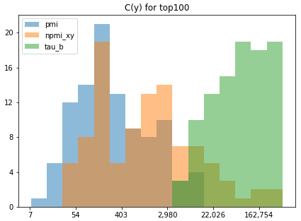
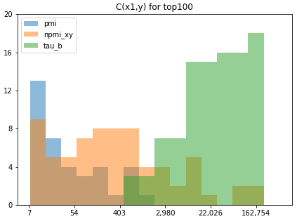
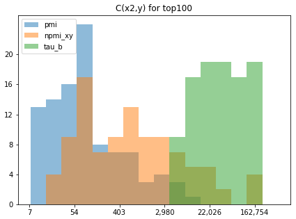
Figure 2. Top 100 count distributions for $PMI$, $nPMI_{xy}$, and $\tau_{b}$

The distribution of $C(y)$, $C(x_{1},y)$, and $C(x_{2},y)$ for the top 100 labels sorted by gap $G(y|x_{1},x_{2},A(\cdot))$ for $PMI$, $nPMI_{xy}$, and $\tau_{b}$. The $x$-axis is the logarithmic-scaled bins and the $y$-axis is the number of labels which have the corresponding count values in that bin.

Similar results were obtained for another cluster of metrics: $DP$, $JI$, and $SDC$. All pairwise comparisons generated linear plots, with about 70% of the top 100 labels shared in common between these metrics when sorted by $G(\cdot)$. Furthermore, about 95% of pairs of those overlapping labels maintained the same relative ranking between metrics. Similar to the $PMI$ cluster, we chose to focus on Demographic Parity ($DP$) as the representative metric from its cluster, due to its mathematical simplicity and prominence in fairness literature.

We next sought to understand how incremental changes to the counts of the labels, $C(y)$, affect these association gap rankings in a real dataset (see Appendix Section E.2). To achieve this, we added a fake label to the real labels of OID, setting initial values for its counts and co-occurences in the dataset, $P(y)$, $P(x_{1},y)$, and $P(x_{2},y)$. Then we incrementally increased or decreased the count of label $y$, and measured whether its bias ranking in $G$ would change relative to the other labels in OID. We repeated this procedure for different orders of magnitude of label count $C(y)$ while maintaining the ratio $P(x_{1},y)/P(x_{2},y)$ as constant.

$\partial p(y)$ $\partial p(x_{1},y)$ $\partial p(x_{2},y)$ $\partial$DP $0$ $\frac{1}{p(x_{1})}$ $\frac{-1}{p(x_{2})}$ $\partial$PMI $0$ $\frac{1}{p(x_{1},y)}$ $\frac{-1}{p(x_{2},y)}$ $\partial nPMI_{y}$ $\frac{ln(\frac{p(x_{2}|y)}{p(x_{1}|y)})}{ln^{2}(p(y))p(y)}$ $\frac{1}{ln(p(y))p(x_{1},y)}$ $\frac{-1}{ln(p(y))p(x_{2},y)}$ $\partial nPMI_{xy}$ $\frac{1}{ln(p(x_{1},y))p(y)}-\frac{1}{ln(p(x_{2},y))p(y)}$ $\frac{ln(p(y))-ln(p(x_{1}))}{ln^{2}(p(x_{1},y))p(x_{1},y)}$ $\frac{ln(p(x_{2}))-ln(p(y))}{ln^{2}(p(x_{2},y))p(x_{2},y)}$ $\partial PMI^{2}$ 0 $\frac{2}{p(x_{1},y)}$ $\frac{-2}{p(x_{2},y)}$ $\partial$SDC see Appendix C $\frac{1}{p(x_{1})+p(y)}$ $\frac{-1}{p(x_{2})+p(y)}$ $\partial$JI see Appendix C $\frac{p(x_{1})+p(y)}{(p(x_{1})+p(y)-p(x_{1},y))^{2}}$ $\frac{p(x_{2})+p(y)}{(p(x_{2})+p(y)-p(x_{2},y))^{2}}$ $\partial$LLR $0$ $\frac{1}{p(x_{1},y)}$ $\frac{-1}{p(x_{2},y)}$ $\partial\tau_{b}$ see Appendix C $\frac{(2-\frac{4}{n})}{\sqrt{(p(x_{1})-p(x_{1})^{2})(p(y)-p(y)^{2})}}$ $\frac{(\frac{4}{n}-2)}{\sqrt{(p(x_{2})-p(x_{2})^{2})(p(y)-p(y)^{2})}}$ $\partial t\mathchar 45\relax test\_gap$ $\frac{\sqrt{p(x_{2})}-\sqrt{p(x_{1})}}{2\sqrt{p(y)}}$ $\frac{1}{\sqrt{p(x_{1})p(y)}}$ $\frac{-1}{\sqrt{p(x_{2})p(y)}}$ This table shows the partial derivatives of the metrics with respect to $P(y)$, $P(x_{1},y)$, and $P(x_{2},y)$. This provides a quantification of the theoretical sensitivity of the metrics for different probability values of $P(y)$, $P(x_{1},y)$, and $P(x_{2},y)$. We see similar experimental results for the metrics with similar orientations (see Appendix).

Table 2. Metric orientations.

This experiment allowed us to determine whether the theoretical sensitivities of each metric to label frequency $P(y)$, as determined by partial derivatives $\partial{A(\cdot)}/\partial{P(y)}$ (see Table 2), would hold in the context of real-world data, where the underlying distribution of label frequencies may not be uniform. If certain subregions of the label distribution are relatively sparse, for example, then the gap ranking of our hypothetical label may not change even if $\partial{A(\cdot)}/\partial{C(y)}\neq 0$. However, in practice we do not observe this behavior in the tested settings (see Appendix for plots of these experiments), where label rank moves with label count roughly as predicted by the partial derivatives in Table 2. In fact, we observed that metrics with larger partial derivatives for $x_{1}$, $x_{2}$, or $y$ often led to a larger change in rank. For example, slightly increasing $P(x_{1},y)$ when $y$ always co-occurs with $x_{1}$, $P(y)=P(x_{1},y)$ affects ranking more for $A=nPMI_{y}$ compared to $A=PMI$ (see Appendix).

4.2. Top 100 Labels by Metric Gaps

When applying these metrics to fairness and bias use cases, model users may be most interested in surfacing the labels with the largest association gaps. If one filters results to a “top K” label set, then the normalization chosen could lead to vastly different sets of labels (e.g., as mentioned earlier, $PMI^{2}$ and $SDC$ only shared 7 labels in their top 100 set for OID).

To further analyze this issue, we calculated simple values for each metric’s top 100 labels sorted by $G(\cdot)$: minimum and maximum values of $C(y)$, $C(x_{1},y)$ and $C(x_{2},y)$ as shown in Table 1. The most salient point is that the clusters of metrics from the Label Ranks subsection also appear to hold in this analysis as well; $PMI$, $PMI^{2}$, and $LLR$ have low $C(y)$, $C(x_{1},y)$ and $C(x_{2},y)$ ranges, whereas $DP$, $JI$, and $SDC$ have relatively high ranges. Another straightforward observation we can make is that the $nPMI_{y}$ and $nPMI_{xy}$ ranges are much broader than the first two clusters, and include the other metrics’ ranges especially for the joint co-occurrences, $C(x_{1},y)$ and $C(x_{2},y)$.

To demonstrate this point more clearly, we plot the distributions of these counts for $PMI$, $nPMI_{xy}$ and $\tau_{b}$ skews in Figure 2 (all other combinations can be found in the Appendix). These three metric distributions show that gap calculations based on $PMI$ (blue distribution) exclusively rank labels with low counts in the top 100 most skewed labels, where $\tau_{b}$ calculations (green distribution) almost exclusively rank labels with much higher counts. The exception is $nPMI_{y}$ and $nPMI_{xy}$ (orange distribution); these two metrics are capable of capturing labels across a range of marginal frequencies. In other words, ranking labels by $PMI$ gaps is likely to highlight rare labels, ranking by $\tau_{b}$ will highlight common labels, and ranking by $nPMI_{xy}$ will highlight both rare and common labels.

An example of this relationship between association metric choice and label commonality can be seen in Table 3 (note, here we use Demographic Parity instead of $\tau_{b}$ because they behave similarly in this respect). In this table, we show the “Top 15 labels” most heavily skewed towards $woman$ relative to $man$ according to $DP$, unnormalized $PMI$, and $nPMI_{xy}$. $DP$ almost exclusively highlights common labels predicted for over 100,000 images in the dataset (e.g., Happiness and Fashion), whereas $PMI$ largely highlights rarer labels predicted for less than 1,000 images (e.g., Treggings and Boho-chic). By contrast, $nPMI_{xy}$ highlights both common and rare labels (e.g., Long Hair as well as Boho-chic).

5. Discussion

Metric $A$	$DP$		$PMI$		$nPMI_{xy}$
Ranks	Label $y$	Count	Label $y$	Count	Label $y$	Count
0		265,853	Dido Flip	140		610
1		270,748	Webcam Model	184	Dido Flip	140
2		221,017	Boho-chic	151		2,906
3		166,186		610	Eye Liner	3,144
4	Beauty	562,445	Treggings	126	Long Hair	56,832
5	Long Hair	56,832	Mascara	539	Mascara	539
6	Happiness	117,562		145	Lipstick	8,688
7	Hairstyle	145,151	Lace Wig	70	Step Cutting	6,104
8	Smile	144,694	Eyelash Extension	1,167	Model	10,551
9	Fashion	238,100	Bohemian Style	460	Eye Shadow	1,235
10	Fashion Designer	101,854		78	Photo Shoot	8,775
11	Iris	120,411	Gravure Idole	200	Eyelash Extension	1,167
12	Skin	202,360		165	Boho-chic	460
13	Textile	231,628	Eye Shadow	1,235	Webcam Model	151
14	Adolescence	221,940		156	Bohemian Style	184

Table 3. Top 15 labels skewed towards $woman$.

Ranking by the gap of label $y$ between $woman$ $x_{1}$ and $man$ $x_{2}$, according to $G(y|x_{1},x_{2},A(\cdot))$. Identity label names are omitted.

In the previous section, we first showed that some association metrics behave very similarly when ranking labels from the Open Images Dataset (OID). We then showed that the mathematical orientations and sensitivity of these metrics align with experimental results from OID. Finally, we showed that the different normalizations affect whether labels with high or low marginal frequencies are likely to be detected as having a significant bias according to $G(y|x_{1},x_{2},A(\cdot))$ in this dataset. We arrive at the conclusion that the $nPMI$ metrics are preferable to other commonly used association metrics in the problem setting of detecting biases without groundtruth labels.

What is the intuition behind this particular association metric as a bias metric? All of the studied entropy-based metrics (gaps in $nPMI$ as well as $PMI$) approximately correspond to whether one identity label $x_{1}$ co-occurs with the target label $y$ more often than another identity label $x_{2}$ relative to chance levels. This chance-level normalization is important because even completely unbiased labels would still co-occur at some baseline rate by chance alone.

The further normalization of $PMI$ by either the marginal or joint probability ($nPMI_{y}$ and $nPMI_{xy}$, respectively) takes this one step further in practice by surfacing labels with larger marginal counts at higher ranks in $G(y|x_{1},x_{2},nPMI)$ alongside labels with smaller marginal counts. This is a somewhat surprising result, because in theory $PMI$ should already be independent of the marginal frequency of $P(y)$ (because $\partial{PMI}/\partial{p(y)}=0$), whereas this derivative for $nPMI$ is non-zero. When we examined this pattern in practice, the labels with smaller counts can achieve very large $P(x_{1},y)$/$P(x_{2},y)$ ratios (and therefore their bias rankings can get very high) merely by reducing the denominator to a single image example. $PMI$ is unable to compensate for this noise, whereas the normalizations we use for $nPMI$ allow us to capture a significant amount of common labels in the top 100 labels by $G(y|x_{1},x_{2},nPMI)$ in spite of this pattern. This result is indicated by the ranges in Table 1 and Figure 2, as well as the set of both common and rare labels for $nPMI$ in Table 3.

Indeed, if the evaluation set is properly designed to match the distribution of use cases of a classification model “in the wild”, then we argue more common labels that have a smaller $P(x_{1},y)$/$P(x_{2},y)$ ratio are still critical to audit for biases. Normalization strategies must be titrated carefully to balance this simple ratio of joint probabilities with the label’s rarity in the dataset.

An alternative solution to this problem could be bucketing labels by their marginal frequency. We argue this is a suboptimal solution for two reasons. First, determining even a single threshold hyperparameter is a painful process for defining fairness constraints. Systems that prevent models from being published if their fairness discrepancies exceed a threshold would then be required to titrate this threshold for every bucket. Secondly, bucketing labels by frequency is essentially a manual and discontinuous form of normalization; we argue that building normalization into the metric directly is a more elegant solution.

Finally, to enable detailed investigation of the model predictions, we implemented and open-sourced a tool to visualize $nPMI$ metrics as a TensorBoard plugin for developers (see Figure 3). It allows users to investigate discrepancies between two or more identity labels and their pairwise comparisons. Users can visualize probabilities, image counts, sample and label distributions, and filter, flag, and download these results.

Figure 3. Open-sourced tool we implemented for bias investigation.

In A, annotations are filtered by an association metric, in this case the $nPMI$ difference ($nPMI\_{gap}$) between $male$ and $female$. In B, distribution of association values. In C, the filtered annotations view. In D, different models or datasets can be selected for display. In E, a parallel coordinates visualization of selected annotations to assess where association differences come from.

6. Conclusion and Future Work

In this paper we have described association metrics that can measure gaps – biases or skews – towards specific labels in the large label space of current computer vision classification models. These metrics do not require ground truth annotations, which allows them to be applied in contexts where it is difficult to apply standard fairness metrics such as Equality of Opportunity (Hardt et al., 2016). According to our experiments, Normalized Pointwise Mutual Information ($nPMI$) is a particularly useful metric for measuring specific biases in a real-world dataset with a large label space, e.g., the Open Images Dataset.

This paper also introduces several questions for future work. The first is whether $nPMI$ is also similarly useful as a bias metric in small label spaces (e.g., credit and loan applications). Second, if we were to have exhaustive ground truth labels for such a dataset, how would the sensitivity of $nPMI$ in detecting biases compare to ground-truth-dependent fairness metrics? Finally, in this work we treated the labels predicted for an image as a flat set. However, just like sentences have rich syntactic structure beyond the “bag-of-words” model in NLP, images also have rich structure and relationships between objects that are not captured by mere rates of binary co-occurrence. This opens up the possibility that within-image label relationships could be leveraged to better understand how concepts are associated in a large computer vision dataset. We leave these questions for future work.

Appendix

The following sections break down all of the different metrics we examined. In Section A, Gap Calculations, we present the calculations of the label association metric gaps, a measurement of the skew with respect to the given sensitive labels $x_{1}$ and $x_{2}$, such as $woman$ $(x_{1})$ and $man$ $(x_{2})$. In Section C, Metric Orientations, we present the derivations to calculate their orientations, which represent the theoretical sensitivities of each metric to various marginal or joint label probabilities.

Appendix A Gap Calculations

• Demographic Parity ($DP$):

  $$DP\_gap=p(y|x_{1})-p(y|x_{2})$$

• Sørensen-Dice Coefficient ($SDC$):

  $$SDC\_gap=\frac{p(x_{1},y)}{p(x_{1})+p(y)}-\frac{p(x_{2},y)}{p(x_{2})+p(y)}$$

• Jaccard Index ($JI$):

  $$JI\_gap=\frac{p(x_{1},y)}{p(x_{1})+p(y)-p(x_{1},y)}-\frac{p(x_{2},y)}{p(x_{2})+p(y)-p(x_{2},y)}$$

• Log-Likelihood Ratio ($LLR$):

  $$LLR\_gap=ln(p(x_{1}|y))-ln(p(x_{2}|y))$$

• Pointwise Mutual Information ($PMI$):

  $$PMI\_gap=ln\left(\frac{p(x_{1},y)}{p(x_{1})p(y)}\right)-ln\left(\frac{p(x_{2},y)}{p(x_{2})p(y)}\right)$$

• Normalized Pointwise Mutual Information, p(y) normalization ($nPMI_{y}$):

  $$nPMI_{y}\_gap=\frac{ln\left(\frac{p(x_{1},y)}{p(x_{1})p(y)}\right)}{ln\left(p(y)\right)}-\frac{ln\left(\frac{p(x_{2},y)}{p(x_{2})p(y)}\right)}{ln\left(p(y)\right)}$$

• Normalized Pointwise Mutual Information, p(x,y) normalization ($nPMI_{xy}$):

  $$nPMI_{xy}\_gap=\frac{ln\left(\frac{p(x_{1},y)}{p(x_{1})p(y)}\right)}{ln\left(p(x_{1},y)\right)}-\frac{ln\left(\frac{p(x_{2},y)}{p(x_{2})p(y)}\right)}{ln\left(p(x_{2},y)\right)}$$

• Squared Pointwise Mutual Information ($PMI^{2}$):

  $$PMI^{2}\_gap=ln\left(\frac{p(x_{1},y)^{2}}{p(x_{1})p(y)}\right)-ln\left(\frac{p(x_{2},y)^{2}}{p(x_{2})p(y)}\right)$$

• Kendall Rank Correlation ($\tau_{b}$):

  $$\tau_{b}=\frac{n_{c}-n_{d}}{\sqrt{(n_{0}-n_{1})(n_{0}-n_{2})}}$$

  $$\tau_{b}\_gap=\tau_{b}(l_{1}=x_{1},l_{2}=y)-\tau_{b}(l_{1}=x_{2},l_{2}=y)$$

• t-test:

  $$t\mathchar 45\relax test\_gap=\frac{p(x_{1},y)-p(x_{1})p(y)}{\sqrt{p(x_{1})p(y)}}-\frac{p(x_{2},y)-p(x_{2})p(y)}{\sqrt{p(x_{2})p(y)}}$$

Appendix B Mathematical Reductions

• PMI:

  (1) $$\begin{split}PMI\_gap=ln\left(\frac{p(x_{1},y)}{p(x_{1})p(y)}\right)-ln\left(\frac{p(x_{2},y)}{p(x_{2})p(y)}\right)\end{split}$$

  (2) $$\begin{split}PMI\_gap=ln\left(\frac{p(x_{1},y)}{p(x_{1})p(y)}.\frac{p(x_{2})p(y)}{p(x_{2},y)}\right)\end{split}$$

  (3) $$\begin{split}PMI\_gap=ln\left(\frac{p(x_{1},y)}{p(x_{1})}.\frac{p(x_{2})}{p(x_{2},y)}\right)\end{split}$$

  (4) $$\begin{split}PMI\_gap=ln\left(\frac{p(y|x_{1})}{p(y|x_{2})}\right)\end{split}$$

  (5) $$\begin{split}PMI\_gap=ln(p(y|x_{1}))-ln(p(y|x_{2}))\end{split}$$

• nPMI p(y) normalization:

  (6) $$\begin{split}nPMI\_gap=\frac{ln\left(\frac{p(x_{1},y)}{p(x_{1})p(y)}\right)}{ln\left(p(y)\right)}-\frac{ln\left(\frac{p(x_{2},y)}{p(x_{2})p(y)}\right)}{ln\left(p(y)\right)}\end{split}$$

  (7) $$\begin{split}nPMI\_gap=\frac{ln(p(y|x_{1}))-ln(p(y|x_{2}))}{ln(p(y))}\end{split}$$

• nPMI p(x,y) normalization:

  (8) $$\begin{split}nPMI\_gap=\frac{ln\left(\frac{p(x_{1},y)}{p(x_{1})p(y)}\right)}{ln\left(p(x_{1},y)\right)}-\frac{ln\left(\frac{p(x_{2},y)}{p(x_{2})p(y)}\right)}{ln\left(p(x_{2},y)\right)}\end{split}$$

  (9) $$\begin{split}nPMI\_gap=ln\left({\left(\frac{p(x_{1},y)}{p(x_{1})p(y)}\right)}^{1/ln(p(x_{1},y))}\right)-ln\left({\left(\frac{p(x_{2},y)}{p(x_{2})p(y)}\right)}^{1/ln(p(x_{2},y))}\right)\end{split}$$

  (10) $$\begin{split}nPMI\_gap=ln\left(\frac{{\left(\frac{p(x_{1},y)}{p(x_{1})p(y)}\right)}^{1/ln(p(x_{1},y))}}{{\left(\frac{p(x_{2},y)}{p(x_{2})p(y)}\right)^{1/ln(p(x_{2},y))}}}\right)\end{split}$$

  (11) $$\begin{split}nPMI\_gap=ln\left(\frac{{\left(\frac{p(x_{1},y)}{p(x_{1})}\right)}^{1/ln(p(x_{1},y))}}{{\left(\frac{p(x_{2},y)}{p(x_{2})}\right)^{1/ln(p(x_{2},y))}}}.{p(y)}^{(1/ln(p(x_{1},y))-1/ln(p(x_{2},y)))}\right)\end{split}$$

  (12) $$\begin{split}nPMI\_gap=ln\left(\frac{{\left(\frac{p(x_{1},y)}{p(x_{1})}\right)}^{1/ln(p(x_{1},y))}}{{\left(\frac{p(x_{2},y)}{p(x_{2})}\right)^{1/ln(p(x_{2},y))}}}\right)+ln\left({p(y)}^{(1/ln(p(x_{1},y))-1/ln(p(x_{2},y)))}\right)\end{split}$$

  (13) $$\begin{split}nPMI\_gap=ln\left(\frac{{p(y|x_{1})}^{1/ln(p(x_{1},y))}}{{p(y|x_{2})^{1/ln(p(x_{2},y))}}}\right)+ln(p(y)).\left(\frac{1}{ln(p(x_{1},y))}-\frac{1}{ln(p(x_{2},y))}\right)\end{split}$$

  (14) $$\begin{split}nPMI\_gap=\frac{ln(p(y|x_{1}))}{ln(p(x_{1},y))}-\frac{ln(p(y|x_{2}))}{ln(p(x_{2},y))}+ln(p(y)).\left(\frac{ln(\frac{p(x_{2},y)}{p(x_{1},y)})}{ln(p(x_{1},y))ln(p(x_{2},y))}\right)\end{split}$$

  (15) $$\begin{split}nPMI\_gap=\frac{ln(p(x_{2}))}{ln(p(x_{2},y))}-\frac{ln(p(x_{1}))}{ln(p(x_{1},y))}+\frac{ln(p(y))ln(\frac{p(x_{2},y)}{p(x_{1},y)})}{ln(p(x_{1},y))ln(p(x_{2},y))}\end{split}$$

  (16) $$\begin{split}nPMI\_gap=\frac{ln(p(x_{2}))}{ln(p(x_{2},y))}-\frac{ln(p(x_{1}))}{ln(p(x_{1},y))}+\frac{ln(p(y))}{ln(p(x_{1},y))}-\frac{ln(p(y))}{ln(p(x_{2},y))}\end{split}$$

• PMI²:

  (18) $$\begin{split}PMI^{2}\_gap=ln\left(\frac{p(x_{1},y)^{2}}{p(x_{1})p(y)}\right)-ln\left(\frac{p(x_{2},y)^{2}}{p(x_{2})p(y)}\right)\end{split}$$

  (19) $$\begin{split}PMI^{2}\_gap=ln\left(\frac{p(x_{1},y)^{2}}{p(x_{1})p(y)}.\frac{p(x_{2})p(y)}{p(x_{2},y)^{2}}\right)\end{split}$$

  (20) $$\begin{split}PMI^{2}\_gap=ln\left(\frac{p(x_{1},y)^{2}}{p(x_{1})}.\frac{p(x_{2})}{p(x_{2},y)^{2}}\right)\end{split}$$

  (21) $$\begin{split}PMI^{2}\_gap=ln\left(\frac{p(y|x_{1})p(x_{1},y)}{p(y|x_{2})p(x_{2},y)}\right)\end{split}$$

  (22) $$\begin{split}PMI^{2}\_gap=ln(p(y|x_{1}))-ln(p(y|x_{2}))+ln(p(x_{1},y))-ln(p(x_{2},y))\end{split}$$

• Kendall Rank Correlation ($\tau_{b}$):
  

  Formal definition:

  $$\tau_{b}=\frac{n_{c}-n_{d}}{\sqrt{(n_{0}-n_{1})(n_{0}-n_{2})}}$$

  • $n_{0}=n(n-1)/2$

  • $n_{1}=\sum_{i}t_{i}(t_{i}-1)/2$

  • $n_{2}=\sum_{j}u_{j}(u_{j}-1)/2$

  • $n_{c}$ is number of concordant pairs

  • $n_{d}$ is number of discordant pairs

  • $n_{c}$ is number of concordant pairs

  • $t_{i}$ is number of tied values in the $i^{th}$ group of ties for the first quantity

  • $u_{j}$ is number of tied values in the $j^{th}$ group of ties for the second quantity

  New notations for our use case:

  $$\tau_{b}(l_{1}=x_{1},l_{2}=y)=\frac{n_{c}(l_{1}=x_{1},l_{2}=y)-n_{d}(l_{1}=x_{1},l_{2}=y)}{\sqrt{({n\choose 2}-n_{s}(l=x_{1}))({n\choose 2}-n_{s}(l=y))}}$$

  • $n_{c}(l_{1},l_{2})={C_{l_{1}=0,l_{2}=0}\choose 2}+{C_{l_{1}=1,l_{2}=1}\choose 2}$

  • $n_{d}(l_{1},l_{2})={C_{l_{1}=0,l_{2}=1}\choose 2}+{C_{l_{1}=1,l_{2}=0}\choose 2}$

  • $n_{s}(l)={C_{l=0}\choose 2}+{C_{l=1}\choose 2}$

  • $C_{conditions}$ is number of examples which satisfies the conditions

  • $n$ number of examples in data set

  (23) $$\begin{split}\tau_{b}(l_{1}=x,l_{2}=y)=\frac{n^{2}(1-2p(x)-2p(y)+2p(x,y)+2p(x)p(y))+n(2p(x)+2p(y)-4p(x,y)-1)}{n^{2}\sqrt{(p(x)-p(x)^{2})(p(y)-p(y)^{2})}}\end{split}$$

  (24) $$\begin{split}\tau_{b}\_gap=\tau_{b}(l_{1}=x_{1},l_{2}=y)-\tau_{b}(l_{1}=x_{2},l_{2}=y)\end{split}$$

Appendix C Metric Orientations

In this section, we derive the orientations of each metric, which can be thought of as the sensitivity of each metric to the given label probability. Table 4 provides a summary, followed by the longer forms.

Table 4. Metric Orientations

	$\partial p(y)$	$\partial p(x_{1},y)$	$\partial p(x_{2},y)$
$\partial$DP	$0$	$\frac{1}{p(x_{1})}$	$\frac{-1}{p(x_{2})}$
$\partial$PMI	$0$	$\frac{1}{p(x_{1},y)}$	$\frac{-1}{p(x_{2},y)}$
$\partial nPMI_{y}$	$\frac{ln(\frac{p(x_{2}|y)}{p(x_{1}|y)})}{ln^{2}(p(y))p(y)}$	$\frac{1}{ln(p(y))p(x_{1},y)}$	$\frac{-1}{ln(p(y))p(x_{2},y)}$
$\partial nPMI_{xy}$	$\frac{1}{ln(p(x_{1},y))p(y)}-\frac{1}{ln(p(x_{2},y))p(y)}$	$\frac{ln(p(y))-ln(p(x_{1}))}{ln^{2}(p(x_{1},y))p(x_{1},y)}$	$\frac{ln(p(x_{2}))-ln(p(y))}{ln^{2}(p(x_{2},y))p(x_{2},y)}$
$\partial PMI^{2}$	0	$\frac{2}{p(x_{1},y)}$	$\frac{-2}{p(x_{2},y)}$
$\partial$SDC	$\frac{p(x_{2},y)}{(p(x_{2})+p(y))^{2}}-\frac{p(x_{1},y)}{(p(x_{1})+p(y))^{2}}$	$\frac{1}{p(x_{1})+p(y)}$	$\frac{-1}{p(x_{2})+p(y)}$
$\partial$JI	$\frac{p(x_{1},y)}{p(x_{1})+p(y)-p(x_{1},y)}-\frac{p(x_{2},y)}{p(x_{2})+p(y)-p(x_{2},y)}$	$\frac{p(x_{1})+p(y)}{(p(x_{1})+p(y)-p(x_{1},y))^{2}}$	$\frac{p(x_{2})+p(y)}{(p(x_{2})+p(y)-p(x_{2},y))^{2}}$
$\partial$LLR	$0$	$\frac{1}{p(x_{1},y)}$	$\frac{-1}{p(x_{2},y)}$
$\partial\tau_{b}$	annoyingly long	$\frac{(2-\frac{4}{n})}{\sqrt{(p(x_{1})-p(x_{1})^{2})(p(y)-p(y)^{2})}}$	$\frac{(\frac{4}{n}-2)}{\sqrt{(p(x_{2})-p(x_{2})^{2})(p(y)-p(y)^{2})}}$
$\partial t\mathchar 45\relax test\_gap$	$\frac{\sqrt{p(x_{2})}-\sqrt{p(x_{1})}}{2\sqrt{p(y)}}$	$\frac{1}{\sqrt{p(x_{1})*p(y)}}$	$\frac{-1}{\sqrt{p(x_{2})*p(y)}}$

• Demographic Parity:

  (25) $$\begin{split}DP\_gap={}&p(y|x_{1})-p(y|x_{2})\end{split}$$

  (26) $$\begin{split}\frac{\partial DP\_gap}{\partial p(y)}={}&0\end{split}$$

  (27) $$\begin{split}\frac{\partial DP\_gap}{\partial p(x_{1},y)}={}&\frac{1}{p(x_{1})}\end{split}$$

  (28) $$\begin{split}\frac{\partial DP\_gap}{\partial p(x_{2},y)}={}&\frac{-1}{p(x_{2})}\end{split}$$

• Sørensen-Dice Coefficient:

  (29) $$\begin{split}SDC\_gap=\frac{p(x_{1},y)}{p(x_{1})+p(y)}-\frac{p(x_{2},y)}{p(x_{2})+p(y)}\end{split}$$

  (30) $$\begin{split}\frac{\partial SDC\_gap}{\partial p(y)}=\frac{p(x_{2},y)}{(p(x_{2})+p(y))^{2}}-\frac{p(x_{1},y)}{(p(x_{1})+p(y))^{2}}\end{split}$$

  (31) $$\begin{split}\frac{\partial SDC\_gap}{\partial p(x_{1},y)}=\frac{1}{p(x_{1})+p(y)}\end{split}$$

  (32) $$\begin{split}\frac{\partial SDC\_gap}{\partial p(x_{2},y)}=\frac{-1}{p(x_{2})+p(y)}\end{split}$$

• Jaccard Index:

  (34) $$\begin{split}JI\_gap=\frac{p(x_{1},y)}{p(x_{1})+p(y)-p(x_{1},y)}-\frac{p(x_{2},y)}{p(x_{2})+p(y)-p(x_{2},y)}\end{split}$$

  (35) $$\begin{split}\frac{\partial JI\_gap}{\partial p(y)}=\frac{p(x_{2},y)}{(p(x_{2})+p(y)-p(x_{2},y))^{2}}-\frac{p(x_{1},y)}{(p(x_{1})+p(y)-p(x_{1},y))^{2}}\end{split}$$

  (36) $$\begin{split}\frac{\partial JI\_gap}{\partial p(x_{1},y)}=\frac{p(x_{1})+p(y)}{(p(x_{1})+p(y)-p(x_{1},y))^{2}}\end{split}$$

  (37) $$\begin{split}\frac{\partial JI\_gap}{\partial p(x_{2},y)}=\frac{p(x_{2})+p(y)}{(p(x_{2})+p(y)-p(x_{2},y))^{2}}\end{split}$$

• Log-Likelihood Ratio:

  (39) $$\begin{split}LLR\_gap=ln(p(x_{1}|y))-ln(p(x_{2}|y))\end{split}$$

  (40) $$\begin{split}\frac{\partial LLR\_gap}{\partial p(y)}=\frac{p(x_{2},y)}{p(x_{2}|y)p(y)^{2}}-\frac{p(x_{1},y)}{p(x_{1}|y)p(y)^{2}}=0\end{split}$$

  (41) $$\begin{split}\frac{\partial LLR\_gap}{\partial p(x_{1},y)}=\frac{1}{p(x_{1}|y)p(y)}=\frac{1}{p(x_{1},y)}\end{split}$$

  (42) $$\begin{split}\frac{\partial LLR\_gap}{\partial p(x_{2},y)}=\frac{-1}{p(x_{2},y)}\end{split}$$

• PMI:

  (44) $$\begin{split}PMI\_gap=ln(p(y|x_{1}))-ln(p(y|x_{2}))\end{split}$$

  (45) $$\begin{split}\frac{\partial PMI\_gap}{\partial p(y)}=0\end{split}$$

  (46) $$\begin{split}\frac{\partial PMI\_gap}{\partial p(x_{1},y)}=\frac{1}{p(x_{1},y)}\end{split}$$

  (47) $$\begin{split}\frac{\partial PMI\_gap}{\partial p(x_{2},y)}=\frac{1}{p(x_{2},y)}\end{split}$$

• PMI²:

  (48) $$\begin{split}PMI^{2}\_gap=ln(p(y|x_{1}))-ln(p(y|x_{2}))+ln(p(x_{1},y))-ln(p(x_{2},y))\end{split}$$

  (49) $$\begin{split}\frac{\partial PMI^{2}\_gap}{\partial p(y)}=0\end{split}$$

  (50) $$\begin{split}\frac{\partial PMI^{2}\_gap}{\partial p(x_{1},y)}=\frac{2}{p(x_{1},y)}\end{split}$$

  (51) $$\begin{split}\frac{\partial PMI^{2}\_gap}{\partial p(x_{2},y)}=\frac{-2}{p(x_{2},y)}\end{split}$$

• nPMI, normalized by p(y) :

  (52) $$\begin{split}nPMI\_gap=\frac{ln(p(y|x_{1}))}{ln(p(y))}-\frac{ln(p(y|x_{2}))}{ln(p(y))}\end{split}$$

  (53) $$\begin{split}\frac{\partial nPMI\_gap}{\partial p(y)}=\frac{ln(p(y|x_{2}))}{ln^{2}(p(y))p(y)}-\frac{ln(p(y|x_{1}))}{ln^{2}(p(y))p(y)}=\frac{ln(\frac{p(x_{2}|y)}{p(x_{1}|y)})}{ln^{2}(p(y))p(y)}\end{split}$$

  (54) $$\begin{split}\frac{\partial nPMI\_gap}{\partial p(x_{1},y)}=\frac{1}{ln(p(y))p(x_{1},y)}\end{split}$$

  (55) $$\begin{split}\frac{\partial nPMI\_gap}{\partial p(x_{2},y)}=\frac{-1}{ln(p(y))p(x_{2},y)}\end{split}$$

• nPMI, normalized by p(x,y) :

  (56) $$\begin{split}nPMI\_gap=\frac{ln(p(x_{2}))}{ln(p(x_{2},y))}-\frac{ln(p(x_{1}))}{ln(p(x_{1},y))}+\frac{ln(p(y))}{ln(p(x_{1},y))}-\frac{ln(p(y))}{ln(p(x_{2},y))}\end{split}$$

  (57) $$\begin{split}\frac{\partial nPMI\_gap}{\partial p(y)}=\frac{1}{ln(p(x_{1},y))p(y)}-\frac{1}{ln(p(x_{2},y))p(y)}\end{split}$$

  (58) $$\begin{split}\frac{\partial nPMI\_gap}{\partial p(x_{1},y)}=\frac{ln(p(y))-ln(p(x_{1}))}{ln^{2}(p(x_{1},y))p(x_{1},y)}\end{split}$$

  (59) $$\begin{split}\frac{\partial nPMI\_gap}{\partial p(x_{1},y)}=\frac{ln(p(x_{2}))-ln(p(y))}{ln^{2}(p(x_{2},y))p(x_{2},y)}\end{split}$$

• Kendall rank correlation ($\tau_{b}$):
  

  (61) $$\begin{split}\tau_{b}\_gap=\tau_{b}(l_{1}=x_{1},l_{2}=y)-\tau_{b}(l_{1}=x_{2},l_{2}=y)\end{split}$$

  (62) $$\begin{split}\frac{\partial\tau_{b}\_gap}{\partial p(x_{1},y)}=\frac{(2-\frac{4}{n})}{\sqrt{(p(x_{1})-p(x_{1})^{2})(p(y)-p(y)^{2})}}\end{split}$$

  (63) $$\begin{split}\frac{\partial\tau_{b}\_gap}{\partial p(x_{2},y)}=\frac{(2-\frac{4}{n})}{\sqrt{(p(x_{2})-p(x_{2})^{2})(p(y)-p(y)^{2})}}\end{split}$$

• $t\mathchar 45\relax test$:
  

  (65) $$\begin{split}t\mathchar 45\relax test\_gap=\frac{p(x_{1},y)-p(x_{1})*p(y)}{\sqrt{p(x_{1})*p(y)}}-\frac{p(x_{2},y)-p(x_{2})*p(y)}{\sqrt{p(x_{2})*p(y)}}\end{split}$$

  (66) $$\begin{split}\frac{\partial t\mathchar 45\relax test\_gap}{\partial p(y)}=\frac{\sqrt{p(x_{2})}-\sqrt{p(x_{1})}}{2\sqrt{p(y)}}\end{split}$$

  (67) $$\begin{split}\frac{\partial t\mathchar 45\relax test\_gap}{\partial p(x_{1},y)}=\frac{1}{\sqrt{p(x_{1})*p(y)}}\end{split}$$

  (68) $$\begin{split}\frac{\partial t\mathchar 45\relax test\_gap}{\partial p(x_{2},y)}=\frac{-1}{\sqrt{p(x_{2})*p(y)}}\end{split}$$

Appendix D Comparison Tables

Table 5. Mean/Std of top 100 Male Association Gaps

Scales of top 100 ($x_{1}=man$)
Metrics	Mean/Std $C(y)$	Mean/Std $C(x_{1},y)$
$DP$	$101.38(\pm 199.32)$	$1.00(\pm 0.00)$
$nPMI_{xy}$	$24371.15(\pm 27597.10)$	$237.92(\pm 604.29)$
$nPMI_{y}$	$75160.45(\pm 119779.13)$	$5680.44(\pm 17193.19)$
$PMI$	$1875.86(\pm 3344.23)$	$2.43(\pm 4.72)$
$PMI^{2}$	$831.43(\pm 620.02)$	$1.09(\pm 0.32)$
$SDC$	$676.33(\pm 412.23)$	$1.00(\pm 0.00)$
$\tau_{b}$	$189294.69(\pm 149505.10)$	$24524.89(\pm 32673.77)$

Table 6. Mean/Std of top 100 Male-Female Association Gaps

Counts for top 100 gaps($x_{1}$=MALE, $x_{2}$=FEMALE)
Metrics	Mean/Std $C(y)$	Mean/Std $C(x_{1},y)$	Mean/Std $C(x_{2},y)$
$DP$	154960.81($\pm$147823.81)	71552.62 ($\pm$67400.44)	70398.07($\pm$56824.32)
$JI$	70403.46 ($\pm$86766.14)	29670.94 ($\pm$35381.09)	35723.13($\pm$39308.46)
$LLR$	1020.60 ($\pm$1971.77)	57.95 ($\pm$178.59)	558.36 ($\pm$1420.15)
$nPMI_{xy}$	13869.42 ($\pm$46244.17)	5771.73 ($\pm$23564.63)	9664.46 ($\pm$31475.19)
$nPMI_{y}$	23156.11 ($\pm$73662.90)	6632.79 ($\pm$25631.26)	10376.39 ($\pm$33559.27)
$PMI$	1020.60 ($\pm$1971.77)	57.95 ($\pm$178.59)	558.36 ($\pm$1420.15)
$PMI^{2}$	1020.60 ($\pm$1971.77)	57.95 ($\pm$178.59)	558.36 ($\pm$1420.15)
$SDC$	67648.20 ($\pm$87258.41)	28193.83 ($\pm$35295.25)	34443.22 ($\pm$39501.21)
$\tau_{b}$	134076.65 ($\pm$144354.70)	53845.80 ($\pm$58016.12)	56032.09 ($\pm$52124.92)

Table 7. Minimum/Maximum of top 100 Male-Female Association Gaps

Metrics	Min/Max $C(y)$	Min/Max $C(x_{1},y)$	Min/Max $C(x_{2},y)$
$PMI$	15 / 10,551	1 / 1,059	8 / 7,755
$PMI^{2}$	15 / 10,551	1 / 1,059	8 / 7,755
$LLR$	15 / 10,551	1 / 1,059	8 / 7,755
$DP$	6,104 / 785,045	628 / 239,950	5,347 / 197,795
$JI$	4,158 / 562,445	399 / 144,185	3,359 / 183,132
$SDC$	2,906 / 562,445	139 / 144,185	2,563 / 183,132
$nPMI_{y}$	35 / 562,445	1 / 144,185	9 / 183,132
$nPMI_{xy}$	34 / 270,748	1 / 144,185	20 / 183,132
$\tau_{b}$	6,104 / 785,045	628 / 207,723	5,347 / 183,132
$t\mathchar 45\relax test$	960 / 562,445	72 / 144,185	870 / 183,132

Appendix E Comparison Plots

E.1. Overall Rank Changes

Table 8. Demographic Parity (di), Jaccard Index (ji), Sørensen-Dice Coefficient (sdc) Comparison

Table 9. Pointwise Mutual Information (pmi), Squared PMI (pmi_2), Log-Likelihood Ratio (ll) Comparison

Table 10. Demographic Parity (di), Pointwise Mutual Information (pmi), Normalized Pointwise Mutual Information (npmi_xy), $\tau_{b}$ (tau_b) Comparison

E.2. Movement plots

Table 11. Demographic Parity (di), Jaccard Index (ji), Sørensen-Dice Coefficient (sdc) Comparison

Table 12. Pointwise Mutual Information (pmi), Squared PMI (pmi_2), Log-Likelihood Ratio (ll) Comparison

Table 13. Demographic Parity (di), Pointwise Mutual Information (pmi), Normalized Pointwise Mutual Information (npmi_xy), $\tau_{b}$ (tau_b) Comparison

Table 14. Example Top Results

	DP		PMI		nPMIxy
Ranks	Label	Count	Label	Count	Label	Count
0	Female	265853	Dido Flip	140		610
1	Woman	270748	Webcam Model	184	Dido Flip	140
2	Girl	221017	Boho-chic	151		2906
3	Lady	166186		610	Eye Liner	3144
4	Beauty	562445	Treggings	126	Long Hair	56832
5	Long Hair	56832	Mascara	539	Mascara	539
6	Happiness	117562		145	Lipstick	8688
7	Hairstyle	145151	Lace Wig	70	Step Cutting	6104
8	Smile	144694	Eyelash Extension	1167	Model	10551
9	Fashion	238100	Bohemian Style	460	Eye Shadow	1235
10	Fashion Designer	101854		78	Photo Shoot	8775
11	Iris	120411	Gravure Idole	200	Eyelash Extension	1167
12	Skin	202360		165	Boho-chic	460
13	Textile	231628	Eye Shadow	1235	Webcam Model	151
14	Adolescence	221940		156	Bohemian Style	184

References

- (1)
- Aletras and Stevenson (2013) Nikolaos Aletras and Mark Stevenson. 2013. Evaluating Topic Coherence Using Distributional Semantics. In Proceedings of the 10th International Conference on Computational Semantics (IWCS 2013) – Long Papers. Association for Computational Linguistics, Potsdam, Germany, 13–22. https://www.aclweb.org/anthology/W13-0102
- Barocas and Selbst (2014) Solon Barocas and Andrew D. Selbst. 2014. Big Data’s Disparate Impact. SSRN eLibrary (2014).
- Berk (2016) Richard Berk. 2016. A primer on fairness in criminal justice risk assessments. The Criminologist 41, 6 (2016), 6–9.
- Bouma (2009) G. Bouma. 2009. Normalized (pointwise) mutual information in collocation extraction.
- Buolamwini and Gebru (2018) Joy Buolamwini and Timnit Gebru. 2018. Gender Shades: Intersectional Accuracy Disparities in Commercial Gender Classification (Proceedings of Machine Learning Research, Vol. 81), Sorelle A. Friedler and Christo Wilson (Eds.). PMLR, New York, NY, USA, 77–91. http://proceedings.mlr.press/v81/buolamwini18a.html
- Burns et al. (2018) Kaylee Burns, Lisa Anne Hendricks, Trevor Darrell, and Anna Rohrbach. 2018. Women also Snowboard: Overcoming Bias in Captioning Models. CoRR abs/1803.09797 (2018). arXiv:1803.09797 http://arxiv.org/abs/1803.09797
- Caliskan et al. (2017) Aylin Caliskan, Joanna J. Bryson, and Arvind Narayanan. 2017. Semantics derived automatically from language corpora contain human-like biases. Science 356, 6334 (2017), 183–186. https://doi.org/10.1126/science.aal4230 arXiv:https://science.sciencemag.org/content/356/6334/183.full.pdf
- Chouldechova (2016) Alexandra Chouldechova. 2016. Fair prediction with disparate impact: A study of bias in recidivism prediction instruments. arXiv:1610.07524 [stat.AP]
- Church and Hanks (1990) Kenneth Ward Church and Patrick Hanks. 1990. Word Association Norms, Mutual Information, and Lexicography. Computational Linguistics 16, 1 (1990), 22–29. https://www.aclweb.org/anthology/J90-1003
- Deng et al. (2009) J. Deng, W. Dong, R. Socher, L.-J. Li, K. Li, and L. Fei-Fei. 2009. ImageNet: A Large-Scale Hierarchical Image Database. In CVPR09.
- Dwork et al. (2011) Cynthia Dwork, Moritz Hardt, Toniann Pitassi, Omer Reingold, and Richard S. Zemel. 2011. Fairness Through Awareness. CoRR abs/1104.3913 (2011). arXiv:1104.3913 http://arxiv.org/abs/1104.3913
- Everingham et al. (2015) Mark Everingham, S. M. Ali Eslami, Luc Van Gool, Christopher K. I. Williams, John Winn, and Andrew Zisserman. 2015. The Pascal Visual Object Classes Challenge: A Retrospective. International Journal of Computer Vision 111, 1 (Jan. 2015), 98–136. https://doi.org/10.1007/s11263-014-0733-5
- Fano (1961) Robert M Fano. 1961. Transmission of information: A statistical theory of communications. American Journal of Physics 29 (1961), 793–794.
- Greenwald et al. (1998) A. G. Greenwald, D. E. McGhee, and J. L. Schwartz. 1998. Measuring individual differences in implicit cognition: the implicit association test. Journal of personality and social psychology 74 (1998). Issue 6.
- Hardt et al. (2016) Moritz Hardt, Eric Price, and Nathan Srebro. 2016. Equality of Opportunity in Supervised Learning. arXiv:1610.02413 [cs.LG]
- Harris (1954) Zellig Harris. 1954. Distributional structure. Word 10, 2-3 (1954), 146–162. https://doi.org/10.1007/978-94-009-8467-7_1
- Jurafsky and Martin (2009) Dan Jurafsky and James H. Martin. 2009. Speech and language processing : an introduction to natural language processing, computational linguistics, and speech recognition. Pearson Prentice Hall, Upper Saddle River, N.J. http://www.amazon.com/Speech-Language-Processing-2nd-Edition/dp/0131873210/ref=pd_bxgy_b_img_y
- Kendall (1938) M. G. Kendall. 1938. A New Measure of Rank Correlation. Biometrika 30, 1-2 (06 1938), 81–93. arXiv:https://academic.oup.com/biomet/article-pdf/30/1-2/81/423380/30-1-2-81.pdf https://doi.org/10.1093/biomet/30.1-2.81
- Kuznetsova et al. (2018) Alina Kuznetsova, Hassan Rom, Neil Alldrin, Jasper R. R. Uijlings, Ivan Krasin, Jordi Pont-Tuset, Shahab Kamali, Stefan Popov, Matteo Malloci, Tom Duerig, and Vittorio Ferrari. 2018. The Open Images Dataset V4: Unified image classification, object detection, and visual relationship detection at scale. CoRR abs/1811.00982 (2018). arXiv:1811.00982 http://arxiv.org/abs/1811.00982
- Lin et al. (2014) Tsung-Yi Lin, Michael Maire, Serge J. Belongie, Lubomir D. Bourdev, Ross B. Girshick, James Hays, Pietro Perona, Deva Ramanan, Piotr Dollár, and C. Lawrence Zitnick. 2014. Microsoft COCO: Common Objects in Context. CoRR abs/1405.0312 (2014). arXiv:1405.0312 http://arxiv.org/abs/1405.0312
- Role and Nadif. (2011) FranÇois Role and Mohamed Nadif. 2011. Handling the Impact of Low Frequency Events on Co-Occurrence Based Measures of Word Similarity - A Case Study of Pointwise Mutual Information. In Proceedings of the International Conference on Knowledge Discovery and Information Retrieval - KDIR, (IC3K 2011). SciTePress, 218–223.
- Russakovsky et al. (2015) Olga Russakovsky, Jia Deng, Hao Su, Jonathan Krause, Sanjeev Satheesh, Sean Ma, Zhiheng Huang, Andrej Karpathy, Aditya Khosla, Michael Bernstein, Alexander C. Berg, and Li Fei-Fei. 2015. ImageNet Large Scale Visual Recognition Challenge. International Journal of Computer Vision (IJCV) 115, 3 (2015), 211–252. https://doi.org/10.1007/s11263-015-0816-y
- Shannon (1948) Claude E. Shannon. 1948. A mathematical theory of communication. Bell Syst. Tech. J. 27, 3 (1948), 379–423. http://dblp.uni-trier.de/db/journals/bstj/bstj27.html#Shannon48
- Snow (2018) Jacob Snow. 2018. Amazon’s Face Recognition Falsely Matched 28 Members of Congress With Mugshots. (2018).
- Spearman (1904) C. Spearman. 1904. The Proof and Measurement of Association Between Two Things. American Journal of Psychology 15 (1904), 88–103.
- Stanford Vision Lab (2020) Stanford Vision Lab. 2020. ImageNet. http://image-net.org/explore (2020). accessed 6.Oct.2020.
- Stock and Cisse (2018) Pierre Stock and Moustapha Cisse. 2018. Convnets and imagenet beyond accuracy: Understanding mistakes and uncovering biases. In Proceedings of the European Conference on Computer Vision (ECCV). 498–512.
- Toglia and Battig (1978) M. P. Toglia and W. F. Battig. 1978. Handbook of semantic word norms. Lawrence Erlbaum.
- Wilson et al. (2019) Benjamin Wilson, Judy Hoffman, and Jamie Morgenstern. 2019. Predictive Inequity in Object Detection. CoRR abs/1902.11097 (2019). arXiv:1902.11097 http://arxiv.org/abs/1902.11097