Unified Robust Training for Graph Neural Networks against Label Noise

Abstract

Graph neural networks (GNNs) have achieved state-of-the-art performance for node classification on graphs. The vast majority of existing works assume that genuine node labels are always provided for training. However, there has been very little research effort on how to improve the robustness of GNNs in the presence of label noise. Learning with label noise has been primarily studied in the context of image classification, but these techniques cannot be directly applied to graph-structured data, due to two major challenges—label sparsity and label dependency—faced by learning on graphs. In this paper, we propose a new framework, UnionNET, for learning with noisy labels on graphs under a semi-supervised setting. Our approach provides a unified solution for robustly training GNNs and performing label correction simultaneously. The key idea is to perform label aggregation to estimate node-level class probability distributions, which are used to guide sample reweighting and label correction. Compared with existing works, UnionNET has two appealing advantages. First, it requires no extra clean supervision, or explicit estimation of the noise transition matrix. Second, a unified learning framework is proposed to robustly train GNNs in an end-to-end manner. Experimental results show that our proposed approach: (1) is effective in improving model robustness against different types and levels of label noise; (2) yields significant improvements over state-of-the-art baselines.

1 Introduction

Nowadays, graph-structured data is being generated across many high-impact applications, ranging from financial fraud detection in transaction networks to gene interaction analysis, from cyber security in computer networks to social network analysis. To ingest rich information on graph data, it is of paramount importance to learn effective node representations that encode both node attributes and graph topology. To this end, graph neural networks (GNNs) have been proposed, built upon the success of deep neural networks (DNNs) on grid-structured data (e.g., images, etc.). GNNs have abilities to integrate both node attributes and graph topology by recursively aggregating node features across the graph. GNNs have achieved state-of-the-art performance on many graph related tasks, such as node classification or link prediction.

The core of GNNs is to learn neural network primitives that generate node representations by passing, transforming, and aggregating node features from local neighborhoods [3]. As such, nearby nodes would have similar node representations [20]. By generalizing convolutional neural networks to graph data, graph convolutional networks (GCNs) [10] define the convolution operation via a neighborhood aggregation function in the Fourier domain. The convolution of GCNs is a special form of Laplacian smoothing on graphs [11], which mixes the features of a node and its nearby neighbors. However, this smoothing operation can be disrupted when the training data is corrupted with label noise. As the training proceeds, GCNs would completely fit noisy labels, resulting in degraded performance and poor generalization. Hence, one key challenge is how to improve the robustness of GNNs against label noise.

Learning with noisy labels has been extensively studied on image classification. Label noise naturally stems from inter-observer variability, human annotator’s error, and errors in crowdsourced annotations [9]. Existing methods attempt to correct the loss function by directly estimating a noise transition matrix [15, 19], or by adding extra layers to model the noise transition matrix [17, 4]. However, it is difficult to accurately estimate the noise transition matrix particularly with a large number of classes. Alternative methods such as MentorNet [8] and Co-teaching [6] seek to separate clean samples from noisy samples, and use only the most likely clean samples to update model training. Other methods [2, 16] reweight each sample in the gradient update of the loss function, according to model’s predicted probabilities. However, they require a large number of labeled samples or an extra clean set for training. Otherwise, reweighting would be unreliable and result in poor performance.

The aforementioned learning techniques, however, cannot be directly applied to tackle label noise on graphs. This is attributed to two significant challenges. (1) Label sparsity: graphs with inter-connected nodes are arguably harder to label than individual images. Very often, graphs are sparsely labeled, with only a small set of labeled nodes provided for training. Hence, we cannot simply drop “bad nodes” with corrupted labels like previous methods using “small-loss trick” [6, 8]. (2) Label dependency: graph nodes exhibit strong label dependency, so nodes with high structural proximity (directly or indirectly connected) tend to have a similar label. This presses a strong need to fully exploit graph topology and sparse node labels when training a robust model against label noise.

To tackle these challenges, we propose a novel approach for robustly learning GNN models against noisy labels under semi-supervised settings. Our approach provides a unified robust training framework for graph neural networks (UnionNET) that performs sample reweighting and label correction simulatenously. The core idea is twofold: (1) leverage random walks to perform label aggregation among nodes with structural proximity. (2) estimate node-level class distribution to guide sample reweighting and label correction. Intuitively, noisy labels could cause disordered predictions around context nodes, thus its derived node class distribution could in turn reflect the reliability of given labels. This provides an effective way to assess the reliability of given labels, guided by which sample reweighting and label correction are expected to weaken unreliable supervision and encourage label smoothing around context nodes. We verify the effectiveness of our proposed approach through experiments and ablation studies on real-world networks, demonstrating its superiority over competitive baselines.

2 Related Work

2.1 Learning with Noisy Labels

Learning with noisy labels has been widely studied in the context of image classification. The first line of research focuses on correcting the loss function, by directly estimating the noise transition matrix between noisy labels and ground true labels [15, 19], or adding an extra softmax layer to estimate the noise transition matrix [17, 4]. However, it is non-trivial to estimate the noise transition matrix accurately. [22] used the negative Box-Cox transformation to improve the robustness of standard cross entropy loss but with worse converging capacity. The second line of approaches seek to separate clean samples from noisy ones, and use only the most likely clean samples to guide network training. MentorNet [8] pre-trains an extra network on a clean set to select clean samples. Co-teaching [6] trains two peer networks to select small-loss samples to train each other. Decoupling [13] updates two networks using only samples with which they disagree. In our setting with very few labeled nodes, we cannot simply drop “bad nodes” as they are still useful to infer the labels of nearby nodes. The third category takes a reweighting approach. [2] utilized a two-component Beta Mixture Model to estimate the probability of a sample being mislabeled, which is used to reweight the sample in the gradient update. It was further improved by combining with mixup augmentation [21]. [16] proposed a meta-learning algorithm that allowed the network to put more weights on the samples with the closest gradient directions with the clean data. Unlike these reweighting methods that rely on the predicted probabilities, our method assigns weights to each node by leveraging topology structure, which is less prone to label noise. Several other methods are concerned with the problem of label correction. [7] chose class prototypes based on sample distance density to correct labels, incurring significant computational overhead. [18] proposed a self-training approach to correct the labels. However, this method discards the original given labels, leading to degraded performance with high noise rates. Our work integrates sample reweighting with label correction, yielding remarkable gains with high noise rates.

2.2 Graph Neural Networks

GNNs have emerged as a new class of deep learning models on graphs. Various types of GNNs, such as GCN [10], graph attention network (GAT) [20], GraphSAGE [5], are proposed in recent years. These models have shown competitive results on node classification, assuming that genuine node labels are provided for training purposes. To date, there has been little research work on robustly training a GNN against label noise. [14] studied the problem of learning GNNs with symmetric label noise. This method adopts a backward loss correction [15] for graph classification. [1] analyzed the robustness of traditional collective node classification methods on graphs (such as label propagation) towards random label noise, but it did not propose new solutions to tackle this problem. To the best of our knowledge, our work is the first to study the problem of learning robust GNNs for semi-supervised node classification on graphs with both symmetric and asymmetric label noise. Our method provides a unified learning framework and does not require explicit estimation of the noise transition matrix.

3 Problem Definition

Given an undirected graph $G=\{\mathcal{V},\mathcal{E},\mathbf{X}\}$, where $\mathcal{V}$ denotes a set of $n$ nodes, and $\mathcal{E}$ denotes a set of edges connecting nodes. $\mathbf{X}=[\mathbf{x}_{1},\mathbf{x}_{2},\ldots,\mathbf{x}_{n}]^{T}\in\mathcal{R}^{n\times d}$ denotes the node feature matrix, where $\mathbf{x}_{i}\in\mathcal{R}^{d}$ is $d$-dimensional feature vector of node $v_{i}$. Let $A\in\mathcal{R}^{n\times n}$ denote the adjacent matrix.

We consider semi-supervised node classification, where only a small fraction of nodes are labeled. Let $\mathcal{L}=\{(\mathbf{x}_{i},\mathbf{y}_{i})\}_{i=1}^{|L|}$ denote the set of labeled nodes, where $\mathbf{x}_{i}$ is feature vector of node $v_{i}$, and $\mathbf{y}_{i}=\{y_{i1},y_{i2},\dots,y_{im}\}$ is the one-hot encoding of node $v_{i}$’s class label, with $y_{ij}\in\{0,1\}$ and $m$ being the number of classes. The rest of nodes belong to the unlabeled set $\mathcal{U}$. Under the GNN learning framework, the aim is to learn a representation $\mathbf{h}_{\mathbf{x}_{i}}$ for each node $v_{i}$ such that its class label can be correctly predicted by $f(\mathbf{h}_{\mathbf{x}_{i}})$. For node classification, the standard cross entropy loss is used as the objective function:

$$\small\mathcal{J}(f(\mathbf{h}_{\mathbf{x}}),\mathbf{y})=-\sum_{i\in|L|}\sum_{j\in m}\mathbf{y}_{ij}\log(f(\mathbf{h}_{\mathbf{x}_{i}})_{j}).$$ (1)

However, when class labels in $\mathcal{L}$ are corrupted with label noise, the standard cross entropy would cause the GNN training to overfit incorrect labels, and in turn lead to degraded classification performance. Therefore, in our work, we aim to train a robust GNN model that is less sensitive to label noise.

Formally, given a small set of noisy labeled nodes $\mathcal{L}$, we aim to: (1) learn node representations $\mathbf{h}$ for all nodes $\mathcal{V}$, and (2) learn a model $f(\mathbf{h})$ to predict the labels of unlabeled nodes in $\mathcal{U}$ with maximum classification performance.

4 The UnionNET Learning Framework

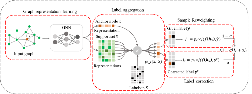
Figure 1: Overview of the UnionNET Framework. The key idea is to infer the reliability of the given labels through estimating node-level class probability distributions via label aggregation. Based on this, the corresponding label weights and corrected labels are obtained to update model parameters during training.

To effectively tackle label noise on graphs, one desirable solution should consider the following key aspects. First, since only a small set of labeled nodes are available for training, we cannot simply drop “bad nodes” using “small-loss trick” [6, 8]. Second, graph nodes that share similar structural context exhibit label dependency. Thus, we propose a unified framework, UnionNET, for robustly training a GNN and performing label correction, as shown in Fig 1.

Taking a given graph as input, a GNN is first applied to learn node representations and generate the predicted label for each node. Then, label information is aggregated to estimate a class probability distribution per node. This aggregation is operated on a support set constructed by collecting context nodes with high structural proximity. According to node-level class probability distributions, our algorithm generates label weights and corrected labels for each labeled node. Those corrected labels generated from the support set could potentially provide extra “correct” supervision. Taken together, both given labels reweighted by label weights and corrected labels are used to update model parameters.

4.1 Label Aggregation

On graphs, it is well studied that nodes with high structural proximity tend to have the same labels [12, 23]. The supervision from noisy labels however disrupt such label smoothness around context nodes. Nevertheless, their smoothness degree could provide a reference to assess the reliability of given labels. Hence, we design a label aggregator that aggregates label information for each labeled node from its context nodes to estimate its class probability distribution. Specifically, we perform random walks to collect context nodes with higher-order proximity. For each labeled node $\hat{\mathbf{x}}\in\mathcal{L}$, called anchor node, we construct a support set of size $k$, denoted as $S=\{(\mathbf{x}_{i},\mathbf{y}_{i})|\hat{\mathbf{x}}\}^{k}$, where $\mathbf{x}_{i}$ is the supportive node in $S$ and $\mathbf{y}_{i}$ is one-hot encoding of $\mathbf{x}_{i}$’s class label. During a random walk, if node $\mathbf{x}_{i}\in\mathcal{L}$, the given label $\mathbf{y}_{i}$ is collected in $S$. Otherwise, the predicted label is used.

Given anchor node $\hat{\mathbf{x}}$ and its support set $\mathcal{S}$, we derive a node-level class probability distribution $P(\mathbf{y}|\hat{\mathbf{x}},S)$ over $m$ classes. It signifies the probabilities of the anchor node belonging to $m$ classes in reference of its support set. Particularly, we specify a non-parametric attention mechanism given by,

$$P(\mathbf{y}|\hat{\mathbf{x}},S)=\sum_{\mathbf{x}_{i}\in S}\mathcal{A}(\hat{\mathbf{x}},\mathbf{x}_{i})\mathbf{y}_{i}=\sum_{\mathbf{x}_{i}\in S}\frac{\exp(\mathbf{h}_{\mathbf{x}_{i}}^{T}\mathbf{h}_{\hat{\mathbf{x}}})}{\sum_{\mathbf{x}_{j}\in S}\exp(\mathbf{h}_{\mathbf{x}_{j}}^{T}\mathbf{h}_{\hat{\mathbf{x}}})}\mathbf{y}_{i}.$$ (2)

Here, the probability of the anchor node belonging to each class is calculated according to its proximity with nearby nodes in the support set. We define the proximity as the inner product in the embedding space, and apply softmax to measure the contribution made by each label in the support set to estimating the anchor node’ class probability distribution. In the support set, if a node has a higher similarity with the anchor node (i.e., higher inner product), its label would contribute more to $P(\mathbf{y}|\hat{\mathbf{x}},S)$, and vice verse. This simple yet effective mechanism estimates a class probability distribution for each node, which is used to guide sample reweighting and label correction.

4.2 Sample Reweighting

For GNNs, the standard cross entropy loss implicitly puts more emphasis on the samples for which the predicted labels disagree with the provided labels during gradient update. This mechanism enables faster convergence and better fitting to the training data. However, if there exist corrupted labels in the training set, this implicit weighting scheme would conversely push the model to overfit noisy labels, leading to degraded performance [22]. To mitigate this, we devise a reweighting scheme for each node according to the reliability of its given label, so that the loss of reliable labels could contribute more during gradient update.

Specifically, we define the reweighting score of anchor node $\hat{\mathbf{x}}$ as:

$$p_{r}(\hat{\mathbf{y}}|\hat{\mathbf{x}},S)=\sum_{\mathbf{x}_{i}\in S,\mathbf{y}_{i}=\hat{\mathbf{y}}}\frac{\exp(\mathbf{h}_{\mathbf{x}_{i}}^{T}\mathbf{h}_{\hat{\mathbf{x}}})}{\sum_{\mathbf{x}_{j}\in S}\exp(\mathbf{h}_{\mathbf{x}_{j}}^{T}\mathbf{h}_{\hat{\mathbf{x}}})}\mathbf{y}_{i}.$$ (3)

The loss function for the labeled nodes is thus defined as:

$$\mathcal{J}_{r}=-\sum_{\hat{\mathbf{x}}\in\mathcal{L}}p_{r}(\hat{\mathbf{y}}|\hat{\mathbf{x}},S)\times\hat{\mathbf{y}}\log(f(\mathbf{h}_{\hat{\mathbf{x}}})),$$ (4)

where $p_{r}(\hat{\mathbf{y}}|\hat{\mathbf{x}},S)$ is the weight imposed on each labeled node $\hat{\mathbf{x}}$ according to the aggregated label information. If the given label $\hat{\mathbf{y}}$ is highly consistent with nearby labels, its gradient would be back-propagated as it is. Otherwise, it would be penalized by the weight during back-propagation.

4.3 Label Correction

The reweighting method reduces the sensitivity of the standard cross entropy to noisy labels, and boosts the robustness of the model. As labeled nodes are limited for training, we also augment the set of labeled nodes by correcting noisy labels. Accordingly, we define the label correction loss as

$$\mathcal{J}_{c}=-\sum_{\hat{\mathbf{x}}\in\mathcal{L}}p_{c}(\mathbf{y}^{c}|\hat{\mathbf{x}},S)\times\mathbf{y}^{c}\log(f(\mathbf{h}_{\hat{\mathbf{x}}})),$$ (5)

$$p_{c}(\mathbf{y}^{c}|\hat{\mathbf{x}},S)=\max_{\mathbf{y}_{i}}P(\mathbf{y}_{i}|\hat{\mathbf{x}},S)=\max_{\mathbf{y}_{i}}\sum_{\mathbf{x}_{i}\in S}\frac{\exp(\mathbf{h}_{\mathbf{x}_{i}}^{T}\mathbf{h}_{\hat{\mathbf{x}}})}{\sum_{\mathbf{x}_{j}\in S}\exp(\mathbf{h}_{\mathbf{x}_{j}}^{T}\mathbf{h}_{\hat{\mathbf{x}}})}\mathbf{y}_{i}.$$ (6)

This provides additional supervision for $\hat{\mathbf{x}}$ with the corrected label $\mathbf{y}^{c}$, encouraging it to have the same label with the most consistent one in its support set. This approach aggregates labels from context nodes via a linear combination based on their similarity in the embedding space. It thus helps diminish the gradient update of corrupted labels, and boosts the supervision from consistent labels.

However, in the presence of extreme label noise, this approach would produce biased correction that deviates far away from its original prior distribution over the training data. This bias could exacerbate the overfitting problem caused by noisy labels. To overcome this, we employ a KL-divergence loss between the prior and predicted distributions to push them as close as possible [18]. It is given by:

$$\mathcal{J}_{p}=\sum_{j=1}^{m}p_{j}\log\frac{p_{j}}{\overline{f(\mathbf{h}_{\mathbf{X}})}_{j}},$$ (7)

Where $p_{j}$ is the prior probability of class $j$ in $\mathcal{L}$, and $\overline{f(\mathbf{h}_{\mathbf{X}})}_{j}=\frac{1}{|L|}\sum_{\mathbf{x}\in\mathcal{L}}f(\mathbf{h}_{\mathbf{x}})_{j}$ is the mean value of predicted probability distribution on the training set.

4.4 Model Training

The training of UnionNET is given in Algorithm 1, which consists of the pre-training phase (Step 1-4) and the training phase (Step 6-11). The pre-training is employed to obtain a parameterized GNN. The pre-trained GNN then generates node representations $\mathbf{h}$, which are used to compute sample weights and corrected labels. After that, model parameters are updated according to the loss function:

$$\mathcal{J}_{f}=(1-\alpha)\mathcal{J}_{r}+\alpha\mathcal{J}_{c}+\beta\mathcal{J}_{p}.$$ (8)

Compared with GNNs with the standard cross entropy loss, the training of UnionNET incurs an extra computational complexity of $\mathcal{O}(|L|ml)$ to estimate node-level class distributions, where $|L|$ is number of labeled nodes, $m$ is number of classes, and $l$ is number of nodes including context nodes in the support set.

Input: Graph $G=\{\mathcal{V},\mathcal{E},\mathbf{X}\}$, node sets ${\mathcal{L},\mathcal{U}}$, $\alpha$, $\beta$

Output: label predictions

1 Initialize network parameters;

2

3for $t=0;t<epoches;t=t+1$ do

4       if $t<$ start_epoch then

5             pre-train the network according to Eq.(1);

6      else

7             Generate node representations $\mathbf{h}_{\mathbf{x}}$;

8             Construct support set S for each node $\hat{\mathbf{x}}\in\mathcal{L}$;

9             Aggregate labels to produce node-level class distribution $P(\mathbf{y}|\hat{\mathbf{x}},S)$;

10             Compute weight $p_{r}(\hat{\mathbf{y}}|\hat{\mathbf{x}},S)$ using Eq.(3);

11             Generate corrected label $\mathbf{y}^{c}$ and its weight $p_{c}(\mathbf{y}^{c}|\hat{\mathbf{x}},S)$ using Eq.(6);

12             Update parameters by descending gradient of Eq.(8)

13      

return Label predictions

Algorithm 1 Robust training for GNNs against label noise

5 Experiments

Datasets and Baselines. Three benchmark datasets are used in our experiments: Cora, Citeseer, and Pubmed. We use the same data split as in [10], with 500 nodes for validation, 1000 nodes for testing, and the remaining for training. Of these training sets, only a small fraction of nodes are labeled (3.6% on Citeseer, 5.2% on Cora, 0.3% on Pubmed) and the rest of nodes are unlabeled. Details about the datasets can be found in [10].

As far as we are concerned, there has not yet been any method exclusively proposed to deal with the label noise problem on GNNs for semi-supervised node classification. We select three strong competing methods from image classification, and adapt them to work with GCN [10] under our setting as baselines.

• Co-teaching [6] trains two peer networks and each network selects the samples with small losses to update the other network.

• Decoupling [13] also trains two networks, but updates model parameters using only the samples with which two networks disagree.

• GCE [22] utilizes a negative Box-Cox transformation as the loss function.

As a general robust training framework, UnionNET can be applied to any semi-supervised GNNs for node classification. Hereby, we instantiate UnionNET with two state-of-the-art GNNs, GCN [10] and GAT [20], denoted as UnionNET-GCN and UnionNET-GAT, respectively.

Experimental Setup. Due to the fact that there are not yet benchmark graph datasets corrupted with noisy labels, we manually generate noisy labels on public datasets to evaluate our algorithm. We follow commonly used label noise generation methods in the domain of images [6, 8]. Given a noise rate $r$, we generate noisy labels over all classes according to a noise transition matrix $Q^{m\times m}$, where $Q_{ij}=p(\tilde{y}=j|y=i)$ is the probability of clean label $\mathbf{y}$ being flipped to noisy label $\tilde{\mathbf{y}}$. We consider two types of noise: 1). Symmetric noise: label $i$ is corrupted to other labels with a uniform random probability, s.t. $Q_{ij}=Q_{ji}$; 2). Pairflip noise: mislabeling only occurs between similar classes. For instance, given $r=0.4$ and $m=3$, the two types of noise transition matrices are given by

$$Q^{\text{symmetric}}=\begin{bmatrix}0.6&0.2&0.2\\ 0.2&0.6&0.2\\ 0.2&0.2&0.6\end{bmatrix};\ \ Q^{\text{pairflip}}=\begin{bmatrix}0.6&0.4&0.\\ 0.&0.6&0.4\\ 0.4&0.&0.6\end{bmatrix}$$

Our experiments follow a transductive setting, where the noise transition matrix is only applied to $\mathcal{L}$, while both validation and test sets are kept clean. For UnionNET-GCN, we apply a two-layer GCN, which has 16 units of hidden layer. The hyper-parameters are set as L2 regularization of $5*10^{-4}$, learning rate of 0.01, dropout rate of 0.5. For UnionNET-GAT, we apply a two-layer GAT, with the first layer consisting of 8 attention heads, each computing 8 features. The learning rate is 0.005, dropout rate is 0.6, L2 regularization is $5*10^{-4}$.

We set the random walk length as 10 on Cora and Citeseer, and 4 on Pubmed, and the random walk is repeated for 10 times for each node to create the support set. We first pre-train the network, during which only the standard cross entropy are used, i.e. $\mathcal{J}_{pre}=\mathcal{J}(f(\mathbf{h}_{\mathbf{x}}),\mathbf{y})$. After that, it proceeds to the formal training, which uses $\mathcal{J}_{f}$ in Eq.(8) as the loss function. And $\alpha$ and $\beta$ are set as 0.5 and 1.0.

5.1 Comparison with State-of-the-art Methods

Table 1: Performance comparison (Micro-F1 score) on node classification

		Symmetric label noise				Asymmetric label noise
Dataset	Methods	noise rate (%)
		10	20	40	60	10	20	30	40
Cora	GCN	0.778	0.732	0.576	0.420	0.768	0.696	0.636	0.517
	Co-teaching	0.775	0.665	0.486	0.249	0.773	0.630	0.542	0.393
	Decoupling	0.738	0.708	0.564	0.436	0.743	0.683	0.574	0.518
	GCE	0.794	0.741	0.621	0.402	0.773	0.714	0.652	0.509
	UnionNET-GCN	0.812	0.795	0.707	0.491	0.801	0.771	0.710	0.584
	GAT	0.755	0.709	0.566	0.389	0.764	0.683	0.616	0.534
	UnionNET-GAT	0.797	0.784	0.692	0.546	0.774	0.745	0.660	0.540
Citeseer	GCN	0.670	0.634	0.480	0.360	0.667	0.624	0.531	0.501
	Co-teaching	0.673	0.541	0.379	0.273	0.677	0.583	0.472	0.418
	Decoupling	0.588	0.584	0.402	0.348	0.615	0.548	0.537	0.468
	GCE	0.690	0.649	0.542	0.358	0.701	0.633	0.552	0.498
	UnionNET-GCN	0.701	0.673	0.567	0.401	0.706	0.667	0.587	0.521
	GAT	0.649	0.604	0.475	0.338	0.651	0.599	0.551	0.480
	UnionNET-GAT	0.695	0.667	0.585	0.424	0.697	0.654	0.604	0.512
Pubmed	GCN	0.748	0.672	0.508	0.367	0.739	0.686	0.618	0.528
	Co-teaching	0.769	0.660	0.478	0.345	0.761	0.634	0.576	0.472
	Decoupling	0.650	0.625	0.422	0.334	0.641	0.592	0.428	0.396
	GCE	0.750	0.699	0.561	0.393	0.753	0.696	0.609	0.567
	UnionNET-GCN	0.769	0.725	0.588	0.409	0.776	0.719	0.649	0.556
	GAT	0.736	0.670	0.525	0.381	0.737	0.657	0.594	0.536
	UnionNET-GAT	0.751	0.726	0.570	0.361	0.758	0.702	0.626	0.552

Table 1 compares the node classification performance of all methods w.r.t. both the symmetric and asymmetric noise types under various noise rates. The best performer is highlighted by bold on each setting. For GCN-based baselines, UnionNET-GCN generally outperforms all baselines by a large margin. Compared with GCN in case of symmetric noise type, UnionNET-GCN achieves an accuracy improvement of 3.4%, 6.3%, 13.1% and 7.1% under the noise rate of 10%, 20%, 40% and 60% on Cora, respectively. Similar improvements can be seen on Citeseer and Pubmed, where the smallest improvement is 2.1% on Pubmed with a noise rate of 10%, and the largest improvement is 8.7% on Citeseer with a noise rate of 40%. In case of asymmetric noise type, UnionNET-GCN has the similar performance. Quantitatively, UnionNET-GCN outperforms GCN by an average of 3.6%, 5.0%, 5.4%, 3.8% on the four noise rates on three datasets.

In most cases, GCE is the second best performer, but its advantage comes at the cost of worse converging capability, leading to sub-optimal performance. Co-teaching and Decoupling do not exhibit robustness towards noisy labels as reported in fully supervised image classification. Their performance drops are expected, as labeled data is further reduced when they prune the training data. This exacerbates the label scarcity problem in our semi-supervised setting.

On three datasets, UnionNET-GAT also surpasses GAT w.r.t. most noise rates. Similar to UnionNET-GCN, UnionNET-GAT generally exhibits greater superiority on higher noise rates. For example, in case of symmetric noise type, UnionNET-GAT outperforms GAT by an average of 3.4%, 6.4%, 9.4% and 7.4% at the four noise rates. Such performance gains validate the generality of UnionNET on improving robustness of different GNN models against noisy labels.

5.2 Ablation Study

We conduct ablation studies to test the effectiveness of different components in UnionNET. Our ablation study is based on GCN, with two ablation versions: 1) UnionNET-R with only sample reweighting; 2) UnionNET-RC with sample reweighting and label correction. The ablation results are summarized in Table 2. When only reweighting is applied, UnionNET-R consistently exhibits advantages over GCN, though the advantageous margins vary over different noise rates and noise types. When it comes to UnionNET-RC, both smaple reweighting and label correction are applied, but, surprisingly, the performance becomes worse than UnionNET-R in some extreme cases with higher noise rates. Therefore, label correction does not guarantee performance gains, whose utility is exerted only with the regularization of the prior distribution loss.

Table 2: Performance comparison of ablation experiments based on GCN

		Symmetric label noise				Asymmetric label noise
Dataset	Methods	noise rate (%)
		10	20	40	60	10	20	30	40
Cora	GCN	0.778	0.732	0.576	0.420	0.768	0.696	0.636	0.517
	UnionNET-R	0.785	0.770	0.659	0.480	0.796	0.709	0.646	0.521
	UnionNET-RC	0.788	0.759	0.626	0.339	0.783	0.703	0.601	0.516
	UnionNET-GCN	0.812	0.795	0.707	0.491	0.801	0.771	0.710	0.584
Citeseer	GCN	0.670	0.634	0.480	0.360	0.667	0.624	0.531	0.501
	UnionNET-R	0.692	0.643	0.507	0.363	0.699	0.627	0.547	0.484
	UnionNET-RC	0.657	0.645	0.495	0.330	0.660	0.642	0.511	0.431
	UnionNET-GCN	0.701	0.673	0.567	0.401	0.706	0.667	0.587	0.521
Pubmed	GCN	0.748	0.672	0.508	0.367	0.739	0.686	0.618	0.528
	UnionNET-R	0.766	0.710	0.573	0.417	0.759	0.705	0.624	0.560
	UnionNET-RC	0.770	0.695	0.573	0.362	0.757	0.650	0.608	0.497
	UnionNET-GCN	0.769	0.725	0.588	0.409	0.776	0.719	0.649	0.556

5.3 Hyper-parameter Sensitivity

We further test the sensitivity of UnionNET-GCN w.r.t. the hyper-parameters ($\alpha$, $\beta$) in Eq.(8) and the random walk length for the support set construction. We report the results on the three datasets at 40% symmetric noise rate in Fig. 2. $\alpha$ controls the trade-off between sample reweighting and label correction. When $\alpha$ is zero, our method is only a reweighting method. When $\alpha$ reaches $1$, our method evolves as a self-learning based label correction method, where given labels are replaced with predicted labels after the initial epoches. On Cora and Citeseer, our method achieves the best results at a medium $\alpha$ value. But on Pubmed, its performance improves as $\alpha$ increases, and reaches its best when $\alpha=1.0$. This is possibly because Pubmed has stronger clustering property with only three classes, enabling the predicted labels to be more reliable for correction. The performance changes w.r.t. $\beta$ exhibits similar trends on the three datasets, where our method gradually improves its performance as $\beta$ increases. The random walk length determines the order of proximity the support set could cover. Either too small or too large of the random walk length would impair the reliability of the supportive nodes, and thus undermine performance improvements. Empirically, our method achieves its best at a medium range of random walk lengths.

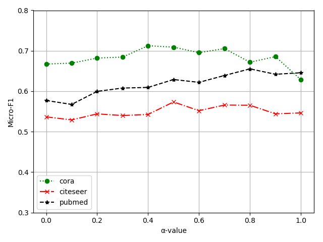
(a) $\alpha$

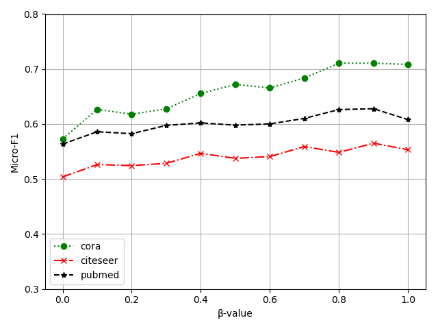
(b) $\beta$

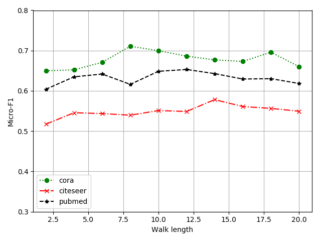
(c) Walk Length

Figure 2: Hyper-parameter sensitivity analysis on $\alpha,\beta$, and the random walk length

6 Conclusion

We proposed a novel semi-supervised framework, UnionNET, for learning with noisy labels on graphs. We argued that, existing methods on image classification fail to work on graphs, as they often take a fully supervised approach, and requires extra clean supervision or explicit estimation of the noise transition matrix. Our approach provides a unified solution to robustly training a GNN model and performing label correction simultaneously. UnionNET is a general framework that can be instantiated with any state-of-the-art semi-supervised GNNs to improve model robustness, and it can be trained in an end-to-end manner. Experiments on three real-world datasets demonstrated that our method is effective in improving model robustness w.r.t. different label noise types and rates, and outperform competitive baselines.

Acknowledgement. This work is supported by the USYD-Data61 Collaborative Research Project grant, the Australian Research Council under Grant DP180100966, and the China Scholarship Council under Grant 201806070131.

References

- [1] de Aquino Afonso, B.K., Berton, L.: Analysis of label noise in graph-based semi-supervised learning. In: SAC. pp. 1127–1134 (2020)
- [2] Arazo, E., Ortego, D., Albert, P., O’Connor, N.E., McGuinness, K.: Unsupervised label noise modeling and loss correction. In: ICML. pp. 312–321 (2019)
- [3] Gilmer, J., Schoenholz, S.S., Riley, P.F., Vinyals, O., Dahl, G.E.: Neural message passing for quantum chemistry. In: ICML. pp. 1263–1272 (2017)
- [4] Goldberger, J., Ben-Reuven, E.: Training deep neural-networks using a noise adaptation layer. In: ICLR (2016)
- [5] Hamilton, W., Ying, Z., Leskovec, J.: Inductive representation learning on large graphs. In: NeurIPS. pp. 1024–1034 (2017)
- [6] Han, B., Yao, Q., Yu, X., Niu, G., Xu, M., Hu, W., Tsang, I., Sugiyama, M.: Co-teaching: Robust training of deep neural networks with extremely noisy labels. In: NeurIPS. pp. 8527–8537 (2018)
- [7] Han, J., Luo, P., Wang, X.: Deep self-learning from noisy labels. In: ICCV. pp. 5138–5147 (2019)
- [8] Jiang, L., Zhou, Z., Leung, T., Li, L.J., Fei-Fei, L.: MentorNet: Learning data-driven curriculum for very deep neural networks on corrupted labels. In: ICML. pp. 2304–2313 (2018)
- [9] Karimi, D., Dou, H., Warfield, S.K., Gholipour, A.: Deep learning with noisy labels: Exploring techniques and remedies in medical image analysis. Medical Image Analysis 65, 101759 (2020)
- [10] Kipf, T.N., Welling, M.: Semi-supervised classification with graph convolutional networks. In: ICLR (2017)
- [11] Li, Q., Han, Z., Wu, X.M.: Deeper insights into graph convolutional networks for semi-supervised learning. In: AAAI. pp. 3538–3545 (2018)
- [12] Lu, Q., Getoor, L.: Link-based classification. In: ICML. pp. 496–503 (2003)
- [13] Malach, E., Shalev-Shwartz, S.: Decoupling “when to update” from “how to update”. In: NeurIPS. pp. 960–970 (2017)
- [14] NT, H., Jin, C., Murata, T.: Learning graph neural networks with noisy labels. In: 2nd ICLR Learning from Limited Labeled Data (LLD) Workshop (2019)
- [15] Patrini, G., Rozza, A., Krishna Menon, A., Nock, R., Qu, L.: Making deep neural networks robust to label noise: A loss correction approach. In: CVPR. pp. 1944–1952 (2017)
- [16] Ren, M., Zeng, W., Yang, B., Urtasun, R.: Learning to reweight examples for robust deep learning. In: ICML. pp. 4334–4343 (2018)
- [17] Sukhbaatar, S., Bruna, J., Paluri, M., Bourdev, L., Fergus, R.: Training convolutional networks with noisy labels. In: ICLR (2014)
- [18] Tanaka, D., Ikami, D., Yamasaki, T., Aizawa, K.: Joint optimization framework for learning with noisy labels. In: CVPR. pp. 5552–5560 (2018)
- [19] Vahdat, A.: Toward robustness against label noise in training deep discriminative neural networks. In: NeurIPS. pp. 5596–5605 (2017)
- [20] Veličković, P., Cucurull, G., Casanova, A., Romero, A., Lio, P., Bengio, Y.: Graph attention networks. In: ICLR (2018)
- [21] Zhang, H., Cisse, M., Dauphin, Y.N., Lopez-Paz, D.: mixup: Beyond empirical risk minimization. ICLR (2018)
- [22] Zhang, Z., Sabuncu, M.: Generalized cross entropy loss for training deep neural networks with noisy labels. In: NeurIPS. pp. 8778–8788 (2018)
- [23] Zhu, X., Ghahramani, Z., Lafferty, J.D.: Semi-supervised learning using gaussian fields and harmonic functions. In: ICML. pp. 912–919 (2003)