Multilevel quasi-Monte Carlo for random elliptic eigenvalue problems II: Efficient algorithms and numerical results

Abstract

Stochastic PDE eigenvalue problems often arise in the field of uncertainty quantification, whereby one seeks to quantify the uncertainty in an eigenvalue, or its eigenfunction. In this paper we present an efficient multilevel quasi-Monte Carlo (MLQMC) algorithm for computing the expectation of the smallest eigenvalue of an elliptic eigenvalue problem with stochastic coefficients. Each sample evaluation requires the solution of a PDE eigenvalue problem, and so tackling this problem in practice is notoriously computationally difficult. We speed up the approximation of this expectation in four ways: we use a multilevel variance reduction scheme to spread the work over a hierarchy of FE meshes and truncation dimensions; we use QMC methods to efficiently compute the expectations on each level; we exploit the smoothness in parameter space and reuse the eigenvector from a nearby QMC point to reduce the number of iterations of the eigensolver; and we utilise a two-grid discretisation scheme to obtain the eigenvalue on the fine mesh with a single linear solve. The full error analysis of a basic MLQMC algorithm is given in the companion paper [Gilbert and Scheichl, 2022], and so in this paper we focus on how to further improve the efficiency and provide theoretical justification for using nearby QMC points and two-grid methods. Numerical results are presented that show the efficiency of our algorithm, and also show that the four strategies we employ are complementary.

1 Introduction

In this paper we develop efficient methods for computing the expectation of an eigenvalue of the stochastic eigenvalue problem (EVP)

$$-\nabla\cdot\big{(}a({\boldsymbol{x}},{\boldsymbol{y}})\,\nabla u({\boldsymbol{x}},{\boldsymbol{y}})\big{)}+b({\boldsymbol{x}},{\boldsymbol{y}})\,u({\boldsymbol{x}},{\boldsymbol{y}}) =\lambda({\boldsymbol{y}})\,c({\boldsymbol{x}},{\boldsymbol{y}})\,u({\boldsymbol{x}},{\boldsymbol{y}}),\ \ \text{for }{\boldsymbol{x}}\in D,$$

$$u({\boldsymbol{x}},{\boldsymbol{y}})\, =\,0\quad \text{for }{\boldsymbol{x}}\in\partial D,$$ (1.1)

where the differential operator $\nabla$ is with respect to ${\boldsymbol{x}}$, which belongs to the physical domain $D\subset\mathbb{R}^{d}$ for $d=1,2,3$. Randomness is incorporated into the PDE (1) through the dependence of the coefficients $a$, $b$ on the stochastic parameter ${\boldsymbol{y}}\,=\,(y_{j})_{j\in\mathbb{N}}$, which is a countably infinite-dimensional vector with i.i.d. uniformly distributed entries: $y_{j}\sim\mathrm{U}[-\frac{1}{2},\frac{1}{2}]$ for $j\in\mathbb{N}$. The whole stochastic parameter domain is denoted by $\Omega\coloneqq[-\tfrac{1}{2},\tfrac{1}{2}]^{\mathbb{N}}$.

The study of stochastic PDE problems is motivated by applications in uncertainty quantification—where one is interested in quantifying how uncertain input data affect model outputs. In the case of (1) the uncertain input data are the coefficients $a$ and $b$, and the outputs of interest are the eigenvalue $\lambda({\boldsymbol{y}})$ and its corresponding eigenfunction $u({\boldsymbol{x}},{\boldsymbol{y}})$, which are now also stochastic objects. As such, to quantify uncertainty we would like to compute statistics of the eigenvalue (or eigenfunction), and in particular, in this paper we compute the expectation of the smallest eigenvalue $\lambda$ with respect to the countable product of uniform densities. This is formulated as the infinite-dimensional integral

$$\mathbb{E}_{\boldsymbol{y}}[\lambda]\,=\,\int_{\Omega}\lambda({\boldsymbol{y}})\,\,\mathrm{d}{\boldsymbol{y}}\,\coloneqq\,\lim_{s\to\infty}\int_{[-\frac{1}{2},\frac{1}{2}]^{s}}\lambda(y_{1},y_{2},\ldots,y_{s},0,0\ldots)\,\,\mathrm{d}y_{1}\,\mathrm{d}y_{2}\cdots\,\mathrm{d}y_{s}\,.$$

EVPs corresponding to differential operators appear in many applications from engineering and the physical sciences, e.g., structural vibration analysis [43], nuclear reactor criticality [14, 27] or photonic crystal structures [13, 29, 34]. In addition, stochastic EVPs, such as (1), have recently garnered more interest due to the desire to quantify the uncertainty present in such applications [41, 2, 44, 3, 38]. Thus, significant development has recently also gone into efficient numerical methods for tackling such stochastic EVPs in practice, the most common being Monte Carlo [41], stochastic collocation [1] and stochastic Galerkin/polynomial chaos methods [16, 44]. The latter two classes perform poorly for high-dimensional problems, so in order to handle the high-dimensionality of the parameter space, sparse and low-rank versions of those methods have been developed, see e.g., [1, 22, 15]. Furthermore, to improve upon classical Monte Carlo, while still performing well in high dimensions, the present authors with their colleagues have analysed the use of quasi-Monte Carlo methods [17, 18].

In practice, for each parameter value ${\boldsymbol{y}}\in\Omega$ the elliptic EVP (1) must be solved numerically, which we do here by the finite element (FE) method, see, e.g., [4]. First, the spatial domain is discretised by a family of triangulations $\{\mathscr{T}_{h}\}_{h>0}$ indexed by the meshsize $h>0$, and then (1) is solved on the finite-dimensional FE space corresponding to $\mathscr{T}_{h}$. This leads to a large, sparse, symmetric matrix EVP, which is typically solved by an iterative method (such as Rayleigh quotient iteration or the Lanczos algorithm, see, e.g., [37, 40]), requiring several solves of a linear system. To speed up the solution of each EVP we use the accelerated two-grid method developed independently in [25, 26] and [47]. In particular, to obtain an eigenvalue approximation corresponding to a “fine” mesh $\mathscr{T}_{h}$, one first solves the FE EVP on a “coarse” mesh $\mathscr{T}_{H}$, with $H\gg h$, to obtain a coarse eigenpair $(\lambda_{H},u_{H})$. An eigenvalue approximation $\lambda^{h}$ on the fine grid $\mathscr{T}_{h}$ is then obtained by performing a single step of shifted inverse iteration with shift $\lambda_{H}$ and start vector $u_{H}$. Typically, the fast convergence rates of FE methods and of shifted inverse iteration for eigenvalue problems allow for a very large difference between the coarse and fine meshsize, e.g., for piecewise polynomial FE spaces it is sufficient to take $H\eqsim h^{1/4}$, so that the cost of the two-grid method essentially reduces to the cost of a single linear solve on the fine mesh. Multilevel sampling schemes also exploit a hierarchy of FE meshes, and so the two-grid method very naturally fits into this framework.

The multilevel Monte Carlo (MLMC) method [20, 23] is a variance reduction scheme that has achieved great success when applied to problems including path integration [23], stochastic differential equations [20] and also stochastic PDEs [6, 8]. For stochastic PDE problems, it is based on a hierarchy of $L+1$ increasingly fine FE meshes $\{\mathscr{T}_{h_{\ell}}\}_{\ell=0}^{L}$ (i,.e., the meshwidths are decreasing $h_{0}>h_{1}>\cdots>h_{L}>0$), and an increasing sequence of truncation dimensions $s_{0}<s_{1}<\cdots<s_{L}<\infty$ of the infinite-dimensional parameter domain $\Omega$. For the eigenvalue problem (1), letting the truncation-FE approximation on level $\ell$ be denoted by $\lambda_{\ell}\coloneqq\lambda_{h_{\ell},s_{\ell}}$, the key idea is to write the expectation on the desired finest level $L$ as a telescoping sum of differences:

$$\mathbb{E}_{\boldsymbol{y}}[\lambda_{L}]\,=\,\mathbb{E}_{\boldsymbol{y}}[\lambda_{0}]+\sum_{\ell=1}^{L}\mathbb{E}_{\boldsymbol{y}}[\lambda_{\ell}-\lambda_{\ell-1}],$$ (1.2)

and then compute each expectation $\mathbb{E}_{\boldsymbol{y}}[\lambda_{\ell}-\lambda_{\ell-1}]$ by an independent MC approximation. As $\ell\to\infty$, provided $h_{\ell}\to 0$ and $s_{\ell}\to\infty$, we have $\lambda_{\ell}\to\lambda$ and hence also $\lambda_{\ell}-\lambda_{\ell-1}\to 0$. Thus the variance on each level decreases, and so less samples will be needed on the finer levels. In this way, the MLMC method achieves a significant cost reduction by spreading the work across the hierarchy of levels, instead of performing all evaluations on the finest level $L$. For any linear functional $\mathcal{G}$, we can write a similar telescoping sum for $\mathbb{E}_{\boldsymbol{y}}[\mathcal{G}(u_{L})]$, where we define $u_{\ell}\coloneqq u_{h_{\ell},s_{\ell}}$. The smallest eigenvalue is simple, therefore we can ensure that the corresponding eigenfunction is unique by normalising it and choosing the sign consistently. Similarly, we normalise each approximation $u_{\ell}$ and choose the sign to match the eigenfunction, which ensures they are also well defined. Our method can also be applied to approximate the expectation of other simple eigenvalues higher up the spectrum, without any essential modifications. If the eigenvalue in question is well-separated from the rest of the spectrum (uniformly in ${\boldsymbol{y}}$) then our analysis can also be extended in a straightforward way. However, for simplicity and clarity of presentation in this paper we focus on the smallest eigenvalue.

Quasi-Monte Carlo methods are equal-weight quadrature rules that are tailored to efficiently approximate high-dimensional integrals, see, e.g., [11, 12]. In particular, by deterministically choosing well-distributed quadrature points, giving preference to more important dimensions, QMC rules can be constructed such that the error converges faster than for MC methods, whilst still being independent of dimension. Using a QMC rule to approximate the expectation on each level in (1.2) instead of Monte Carlo gives a Multilevel quasi-Monte Carlo (MLQMC) method. MLQMC methods were first developed in [21] for option pricing, and since then have also had great success for UQ in stochastic PDE problems [19, 32, 31]. The gains are complementary, so that for several problems MLQMC methods can be shown to result in faster convergence than either MLMC methods or single level QMC approximations.

In this paper, we present an efficient MLQMC method for computing the expectation of the smallest eigenvalue of stochastic eigenvalue problems of the form (1). We employ four complementary strategies: 1) we use the ML strategy to reduce the variance and spread the work across a hierarchy of FE meshes and truncation dimensions; 2) we use QMC methods to compute the expectation on each level more efficiently; 3) we use the two-grid method for eigenvalue problems [25, 26, 47] to compute the eigenpair on finer grids using an eigensolve on a very coarse grid followed by a single linear solve; and 4) we reuse the eigenvector corresponding to a nearby QMC point as the starting vector for the Rayleigh quotient algorithm to solve each eigenvalue problem.

The focus of this paper is on developing the above practical strategies to give an efficient MLQMC method. A rigorous analysis of MLQMC methods for the stochastic EVP (1) is the focus of a separate paper [19]. However, we do give a theoretical justification of the enhancement strategies 3) and 4). First, we extend the two-grid method and its analysis to stochastic EVPs, allowing also for a reduced truncation dimension on the “coarse grid”. Second, we analyse the benefit of using an eigenvector corresponding to a nearby QMC point as the starting vector for the iterative eigensolve.

The structure of the paper is as follows. In Section 2 we present the necessary background material. Then in Section 3 we extend the two-grid method for deterministic EVPs to stochastic EVPs and analyse the error. In Section 4 we describe a basic MLQMC algorithm, and then outline how one can reduce the cost by using two-grid methods and nearby QMC points. Finally, in Section 5 we present numerical results for two test problems.

2 Mathematical background

In this section we briefly summarise the relevant material on variational EVPs, two-grid FE methods and QMC methods. For further details we refer the reader to the references indicated throughout or to [17].

We make the following assumptions on the physical domain and on the boundedness of the coefficients (from above and below). These ensure the well-posedness of (1) and admit a fast convergence rate of our MLQMC algorithm.

Assumption A 1.

1. $D\subset\mathbb{R}^{d}$, for $d=1,2,3$, is bounded and convex.

2. $a$ and $b$ are of the form

   $$a({\boldsymbol{x}},{\boldsymbol{y}})=a_{0}({\boldsymbol{x}})+\sum_{j=1}^{\infty}y_{j}a_{j}({\boldsymbol{x}})\quad\text{and}\quad b({\boldsymbol{x}},{\boldsymbol{y}})=b_{0}({\boldsymbol{x}})+\sum_{j=1}^{\infty}y_{j}b_{j}({\boldsymbol{x}})\,,$$ (2.1)

   where $a_{j},\ b_{j}\in L^{\infty}(D)$, for all $j\geq 0$, and $c\in L^{\infty}(D)$ depend on ${\boldsymbol{x}}$ but not ${\boldsymbol{y}}$.

3. There exists $a_{\min}>0$ such that $a({\boldsymbol{x}},{\boldsymbol{y}})\geq a_{\min}$, $b({\boldsymbol{x}},{\boldsymbol{y}})\geq 0$ and $c({\boldsymbol{x}})\geq a_{\min}$, for all ${\boldsymbol{x}}\in D$, ${\boldsymbol{y}}\in\Omega$.

4. There exists $p\in(0,1)$ and $q\in(0,1)$ such that

   $$\sum_{j=1}^{\infty}\max\big{(}\|a_{j}\|_{L^{\infty}},\,\|b_{j}\|_{L^{\infty}}\big{)}^{p}<\infty\quad\text{and}\quad\sum_{j=1}^{\infty}\|\nabla a_{j}\|_{L^{\infty}}^{q}\,<\,\infty\,.$$

For convenience, we then let $a_{\max}<\infty$ be such that

$$\max\big{\{}\|a({\boldsymbol{y}})\|_{L^{\infty}},\|\nabla a({\boldsymbol{y}})\|_{L^{\infty}},\|b({\boldsymbol{y}})\|_{L^{\infty}},\|c\|_{L^{\infty}}\big{\}}\,\leq\,a_{\max},\quad\text{for all }{\boldsymbol{y}}\in\Omega.$$ (2.2)

2.1 Variational eigenvalue problems

For the variational form of the EVP (1), we introduce the usual function space setting for second-order elliptic PDEs: the first-order Sobolev space of functions with zero trace is denoted by $V\coloneqq H^{1}_{0}(D)$ and equipped with the norm $\|v\|_{V}\coloneqq\|\nabla v\|_{L^{2}}$. Its dual space is $V^{*}\coloneqq H^{-1}(D)$. We will also use the Lebesgue space $L^{2}(D)$, equipped with the usual inner product $\langle\cdot,\cdot\rangle_{L^{2}}$, and the induced norm $\|\cdot\|_{L^{2}}$.

Next, for each ${\boldsymbol{y}}\in\Omega$ define the bilinear form $\mathcal{A}({\boldsymbol{y}}):V\times V\to\mathbb{R}$ by

$$\mathcal{A}({\boldsymbol{y}};w,v)\,\coloneqq\,\int_{D}a({\boldsymbol{x}},{\boldsymbol{y}})\nabla w({\boldsymbol{x}})\cdot\nabla v({\boldsymbol{x}})\,\mathrm{d}{\boldsymbol{x}}+\int_{D}b({\boldsymbol{x}},{\boldsymbol{y}})w({\boldsymbol{x}})v({\boldsymbol{x}})\,\mathrm{d}{\boldsymbol{x}},$$

which is also an inner product on $V$ and admits the induced norm $\|v\|_{\mathcal{A}({\boldsymbol{y}})}\coloneqq\sqrt{\mathcal{A}({\boldsymbol{y}};v,v)}$. We define also the inner product $\mathcal{M}:V\times V\to\mathbb{R}$ by

$$\mathcal{M}(w,v)\,\coloneqq\,\int_{D}c({\boldsymbol{x}})w({\boldsymbol{x}})v({\boldsymbol{x}})\,\mathrm{d}{\boldsymbol{x}}\,,$$

again with induced norm given by $\|v\|_{\mathcal{M}}\coloneqq\sqrt{\mathcal{M}(v,v)}$. Further, let $\mathcal{M}(\cdot,\cdot)$ also denote the duality paring on $V\times V^{*}$.

The variational form of the EVP (1) is: Find $\lambda({\boldsymbol{y}})\in\mathbb{R}$, $u({\boldsymbol{y}})\in V$ such that

$$\mathcal{A}({\boldsymbol{y}};u({\boldsymbol{y}}),v)\, =\,\lambda({\boldsymbol{y}})\mathcal{M}(u({\boldsymbol{y}}),v)\quad\text{for all }v\in V\,,$$ (2.3)

$$\|u({\boldsymbol{y}})\|_{\mathcal{M}}\, =\,1.$$

The variational EVP (2.3) is symmetric and so it is well-known that (2.3) admits countably many, strictly positive eigenvalues, see, e.g., [4]. The eigenvalues – labelled in ascending order, counting multiplicities – and the corresponding eigenfunctions are denoted by

$$0\,<\,\lambda_{1}({\boldsymbol{y}})\,\leq\,\lambda_{2}({\boldsymbol{y}})\,\leq\,\cdots,\quad\text{and}\quad u_{1}({\boldsymbol{y}}),\ u_{2}({\boldsymbol{y}}),\ \ldots\,.$$

For ${\boldsymbol{y}}\in\Omega$, we define the solution operator $T=T({\boldsymbol{y}}):V^{*}\to V$ by

$$\mathcal{A}({\boldsymbol{y}};Tf,v)\,=\,\mathcal{M}(f,v)\quad\text{for all }v\in V.$$

Clearly, if $\lambda({\boldsymbol{y}})$ is an eigenvalue of (2.3) then $\mu({\boldsymbol{y}})=1/\lambda({\boldsymbol{y}})$ is an eigenvalue of $T$ and the corresponding eigenspaces are the same.

The Krein–Rutmann Theorem ensures the smallest eigenvalue is simple, and then in [17, Prop. 2.4] it was shown that the spectral gap can be bounded away from 0 independently of ${\boldsymbol{y}}$. That is, there exists $\rho>0$, independent of ${\boldsymbol{y}}$, such that

$$\lambda_{2}({\boldsymbol{y}})-\lambda_{1}({\boldsymbol{y}})\,\geq\,\rho\quad\text{for all }{\boldsymbol{y}}\in\Omega.$$ (2.4)

The eigenfunctions $\{u({\boldsymbol{y}})\}_{k\in\mathbb{N}}$ can be chosen to form a basis for $V$ that is orthonormal with respect to $\mathcal{M}(\cdot,\cdot)$, and hence, by (2.3), also orthogonal with respect to $\mathcal{A}({\boldsymbol{y}};\cdot,\cdot)$. For ${\boldsymbol{y}}\in\Omega$, let the eigenspace $E(\lambda_{k}({\boldsymbol{y}}))$ be the subspace spanned by all eigenfunctions corresponding to $\lambda_{k}({\boldsymbol{y}})$, and let $\widehat{E}(\lambda_{k}({\boldsymbol{y}}))\coloneqq\{v:v\in E(\lambda_{k}({\boldsymbol{y}})),\|v\|_{V}=1\}$.

Since the coefficients are uniformly bounded away from 0 and from above, the $\mathcal{A}({\boldsymbol{y}})$- and $\mathcal{M}$-norms are equivalent to the $V$- and $L^{2}$-norms, respectively, with

$$c_{\mathcal{A}}\|v\|_{V}\,\leq\, \|v\|_{\mathcal{A}({\boldsymbol{y}})}\,\leq\,C_{\mathcal{A}}\|v\|_{V}\,,$$ (2.5)

$$c_{\mathcal{M}}\|v\|_{L^{2}}\,\leq\, \|v\|_{\mathcal{M}}\,\leq\,C_{\mathcal{M}}\|v\|_{L^{2}},$$ (2.6)

where the constants are independent of ${\boldsymbol{y}}$, see [19, eqs. (2.7), (2.8)] for their explicit values. By $C_{\mathrm{Poin}}>0$ we denote the Poincaré constant, which is independent of ${\boldsymbol{y}}$ and such that

$$\|v\|_{L^{2}(D)}\,\leq\,C_{\mathrm{Poin}}\|v\|_{V},\quad\text{for all }v\in V.$$ (2.7)

For the remainder of the paper we denote the smallest eigenvalue and its corresponding eigenfunction by $\lambda=\lambda_{1}$ and $u=u_{1}$, respectively.

2.2 Stochastic dimension truncation

In order to evaluate the stochastic coefficients $a({\boldsymbol{y}})$ and $b({\boldsymbol{y}})$ in practice, we must first truncate the infinite-dimensional stochastic domain $\Omega$. This is done by choosing a finite truncation dimension $s\in\mathbb{N}$ and by setting $y_{j}=0$ for all $j>s$. We define the following notation: ${\boldsymbol{y}}_{s}=(y_{1},y_{2},\ldots,y_{s})$,

$$a^{s}({\boldsymbol{x}},{\boldsymbol{y}})\,\coloneqq\,a_{0}({\boldsymbol{x}})+\sum_{j=1}^{s}y_{j}a_{j}({\boldsymbol{x}})\quad\text{and}\quad b^{s}({\boldsymbol{x}},{\boldsymbol{y}})\,\coloneqq\,b_{0}({\boldsymbol{x}})+\sum_{j=1}^{s}y_{j}b_{j}({\boldsymbol{x}}).$$

In this way, the truncated coefficients $a^{s}({\boldsymbol{y}})$ and $b^{s}({\boldsymbol{y}})$ can be evaluated in practice, since they only depend on finitely many terms.

Similarly, the truncated approximations of the eigenvalue and eigenfunction are denoted by $\lambda_{s}({\boldsymbol{y}}),u_{s}({\boldsymbol{y}})$, respectively. Defining the bilinear form $\mathcal{A}_{s}({\boldsymbol{y}}):V\times V\to\mathbb{R}$ corresponding to the truncated coefficients by

$$\mathcal{A}_{s}({\boldsymbol{y}};w,v)\,\coloneqq\int_{D}a^{s}({\boldsymbol{x}},{\boldsymbol{y}})\nabla w({\boldsymbol{x}})\cdot\nabla v({\boldsymbol{x}})\,\mathrm{d}{\boldsymbol{x}}+\int_{D}b^{s}({\boldsymbol{x}},{\boldsymbol{y}})w({\boldsymbol{x}})v({\boldsymbol{x}})\,\mathrm{d}{\boldsymbol{x}}\,,$$ (2.8)

we have that $\lambda_{s}({\boldsymbol{y}}),u_{s}({\boldsymbol{y}})$ satisfy

$$\mathcal{A}_{s}({\boldsymbol{y}};u_{s}({\boldsymbol{y}}),v)\,=\,\lambda_{s}({\boldsymbol{y}})\mathcal{M}(u_{s}({\boldsymbol{y}}),v),\quad\text{for all }v\in V\,.$$ (2.9)

2.3 Finite element methods for eigenvalue problems

The eigenvalue problem (2.3) will be discretised in the spatial domain using piecewise linear finite elements (FE). First, we partition the spatial domain $D$ using a family of shape regular triangulations $\{\mathscr{T}_{h}\}_{h>0}$, indexed by the meshwidth $h=\max\{\mathrm{diam}(\tau):\tau\in\mathscr{T}_{h}\}$.

Then, for $h>0$ let $V_{h}$ be the conforming FE space of continuous functions that are piecewise linear on the elements of the triangulation $\mathscr{T}_{h}$, and let $M_{h}\coloneqq\dim(V_{h})<\infty$ denote the dimension of this space. Additionally, we assume that each mesh $\mathscr{T}_{h}$ is such that the dimension of the corresponding FE space $V_{h}$ is

$$M_{h}\eqsim h^{-d},$$ (2.10)

which will be satisfied by quasi-uniform meshes, but also allows for locally refined meshes.

For each ${\boldsymbol{y}}\in\Omega$, the FE eigenvalue problem is: Find $\lambda_{h}({\boldsymbol{y}})\in\mathbb{R}$, $u_{h}({\boldsymbol{y}})\in V_{h}$ such that

$$\mathcal{A}({\boldsymbol{y}};u_{h}({\boldsymbol{y}}),v_{h})\, =\,\lambda_{h}({\boldsymbol{y}})\mathcal{M}(u_{h}({\boldsymbol{y}}),v_{h})\quad\text{for all }v_{h}\in V_{h}\,,$$ (2.11)

$$\|u_{h}({\boldsymbol{y}})\|_{\mathcal{M}}\, =\,1.$$

The FE eigenvalue problem (2.11) admits $M_{h}$ eigenvalues and corresponding eigenvectors

$$0\,<\,\lambda_{1,h}({\boldsymbol{y}})\,\leq\,\lambda_{2,h}({\boldsymbol{y}})\,\leq\,\cdots\,\leq\,\lambda_{M_{h},h}({\boldsymbol{y}})\,,\quad\text{and}\quad u_{1,h}({\boldsymbol{y}}),\ u_{2,h}({\boldsymbol{y}}),\ \ldots,\ u_{M_{h},h}({\boldsymbol{y}})\,,$$

which converge from above to the first $M_{h}$ eigenvalues and eigenfunctions of (2.3) as $h\to 0$, see, e.g., [4] or [17] for the stochastic case.

As before, let $E(\lambda_{k,h}({\boldsymbol{y}}))$ be the eigenspace corresponding to $\lambda_{k,h}({\boldsymbol{y}})$ and define $\widehat{E}(\lambda_{k,h}({\boldsymbol{y}}))\coloneqq\{v\in E(\lambda_{k,h}({\boldsymbol{y}})):\|v\|_{V}=1\}$. If the exact eigenvalue $\lambda_{k}({\boldsymbol{y}})$ has multiplicity $m$ (and we assume without loss of generality that $\lambda_{k}({\boldsymbol{y}})=\lambda_{k+1}({\boldsymbol{y}})=\cdots=\lambda_{k+m-1}({\boldsymbol{y}})$), then there exist $m$ FE eigenvalues, $\lambda_{k,h}({\boldsymbol{y}}),$ $\lambda_{k+1,h}({\boldsymbol{y}}),\ldots,\lambda_{k+m-1,h}({\boldsymbol{y}})$, that converge to $\lambda_{k}({\boldsymbol{y}})$, but are not necessarily equal. As such, we also define $E_{h}(\lambda_{k}({\boldsymbol{y}}))$ to be the direct sum of all the eigenspaces $E(\lambda_{\ell,h}({\boldsymbol{y}}))$ such that $\lambda_{\ell,h}({\boldsymbol{y}})\to\lambda_{k}({\boldsymbol{y}})$. Finally, we define $\widehat{E}_{h}(\lambda_{k}({\boldsymbol{y}})\coloneqq\{v\in E_{h}(\lambda_{k}({\boldsymbol{y}})):\|v\|_{V}=1\}$.

In Assumption A1 we have only assumed that the physical domain $D$ is convex and that $a\in W^{1,\infty}(D)$. Hence, piecewise linear FEs are sufficient to achieve the optimal rates of convergence with respect to $h$ in general. In particular, in [17, Thm. 2.6] it was shown that the FE error for the minimal eigenpair can be bounded independently of ${\boldsymbol{y}}$ with the usual rates in terms of $h$. Explicitly, if $h>0$ is sufficiently small, then for all ${\boldsymbol{y}}\in\Omega$

$$\|u({\boldsymbol{y}})-u_{h}({\boldsymbol{y}})\|_{V}\, \leq\,C_{u}h,\qquad|\lambda({\boldsymbol{y}})-\lambda_{h}({\boldsymbol{y}})|\,\leq\,C_{\lambda}h^{2},$$ (2.12)

and for $\mathcal{G}\in H^{-1+t}(D)$ with $t\in[0,1]$

$$\big{|}\mathcal{G}(u({\boldsymbol{y}}))-\mathcal{G}(u_{h}({\boldsymbol{y}}))\big{|}\,\leq\,C_{\mathcal{G}}\,h^{1+t}\,,$$ (2.13)

where $0<C_{\lambda},\ C_{u},\ C_{\mathcal{G}}<\infty$ are independent of ${\boldsymbol{y}}$ and $h$.

In the companion paper [19], it is shown that for $h$ sufficiently small the spectral gap of the FE eigenvalue problem (2.11) satisfies the uniform lower bound

$$\lambda_{2,h}({\boldsymbol{y}})-\lambda_{1,h}({\boldsymbol{y}})\,\geq\,\frac{\rho}{2}\,>\,0,$$ (2.14)

and that the eigenvalues and eigenfunctions of both (2.3) and (2.11) satisfy the bounds

$$\underline{\lambda_{k}}\,\leq\,\lambda_{k}({\boldsymbol{y}})\,\leq\,\lambda_{k,h}({\boldsymbol{y}})\, \leq\,\overline{\lambda_{k}},\quad\text{and}$$ (2.15)

$$\max\big{\{}\|u_{k}({\boldsymbol{y}})\|_{V},\ \|u_{k,h}({\boldsymbol{y}})\|_{V}\big{\}}\, \,\leq\,\overline{u_{k}},$$ (2.16)

where $\underline{\lambda_{k}},\overline{\lambda_{k}},\overline{u_{k}}$ are also independent of both ${\boldsymbol{y}}$ and $h$.

Note that the use of piecewise linear FEs is not a restriction on our MLQMC methods. The algorithms presented in Section 4 are very general, and will work with higher order FE methods as well, without any modification of the overall algorithm structure.

2.4 Iterative solvers for eigenvalue problems

The discrete EVP (2.11) from the previous section leads to a generalised matrix EVP of the form $A_{h}{\boldsymbol{u}}_{h}=\lambda_{h}B_{h}{\boldsymbol{u}}_{h}$, where, in general, the matrices $A_{h}$ and $B_{h}$ are large, sparse and symmetric positive definite.

Since we are only interested in computing a single eigenpair, we will use Rayleigh quotient (RQ) iteration to compute it. It is well-known that for symmetric matrices RQ iteration converges cubically for almost all starting vectors, see, e.g., [37].

2.5 Quasi-Monte Carlo integration

A quasi-Monte Carlo (QMC) method is an equal weight quadrature rule

$$Q_{s,N}f\,=\,\frac{1}{N}\sum_{k=0}^{N-1}f({\boldsymbol{t}}_{k})$$ (2.17)

with $N\in\mathbb{N}$ deterministically-chosen quadrature points $\{{\boldsymbol{t}}_{k}\}_{k=0}^{N-1}$, as opposed to random quadrature points as in Monte Carlo. The key feature of QMC methods is that the points are cleverly constructed to be well-distributed within high-dimensional domains, which allows for efficient approximation of high-dimensional integrals such as

$$\mathcal{I}_{s}f\,\coloneqq\,\int_{[-\frac{1}{2},\frac{1}{2}]^{s}}f({\boldsymbol{y}})\,\mathrm{d}{\boldsymbol{y}}\,.$$

There are many different types of QMC point sets, and for further details we refer the reader to, e.g., [11].

In this paper, we use a simple to construct, yet powerful, class of QMC methods called randomly shifted rank-1 lattice rules. A randomly shifted lattice rule approximation to $\mathcal{I}_{s}f$ using $N$ points is given by

$$Q_{s,N}({\boldsymbol{\Delta}})f\,\coloneqq\,\frac{1}{N}\sum_{k=0}^{N-1}f(\{t_{k}+{\boldsymbol{\Delta}}\}-\tfrac{\boldsymbol{1}}{\boldsymbol{2}})$$ (2.18)

where ${\boldsymbol{z}}\in\mathbb{N}^{s}$ is the generating vector and the points ${\boldsymbol{t}}_{k}$ are given by

$${\boldsymbol{t}}_{k}=\bigg{\{}\frac{k{\boldsymbol{z}}}{N}\bigg{\}}\quad\text{for }k=0,1,\ldots,N-1\,,$$

${\boldsymbol{\Delta}}\in[0,1)^{s}$ is a uniformly distributed random shift, and $\{\cdot\}$ denotes the fractional part of each component of a vector. Note that we have subtracted $1/2$ in each dimension to shift the quadrature points from $[0,1]^{s}$ to $[-\frac{1}{2},\frac{1}{2}]^{s}$.

Good generating vectors can be constructed in practice using the component-by-component (CBC) algorithm, or the more efficient Fast CBC construction [35, 36]. In fact, it can be shown that for functions in certain first-order weighted Sobolev spaces such as those introduced in [42], the root-mean-square (RMS) error of a randomly shifted lattice rule using a CBC-constructed generating vector achieves almost the optimal rate of $\mathcal{O}(N^{-1})$.

To state the CBC error bound, we briefly introduce the following specific class of weighted Sobolev spaces, which are useful for the analysis of lattice rules. Given a collection of weights ${\boldsymbol{\gamma}}\coloneqq\{\gamma_{\mathrm{\mathfrak{u}}}>0:{\mathrm{\mathfrak{u}}}\subseteq\{1,2,\ldots,s\}\}$, which represent the importance of different subsets of variables, let $\mathcal{W}_{s,{\boldsymbol{\gamma}}}$ be the $s$-dimensional weighted (unanchored) Sobolev space of functions with square-integrable mixed first derivatives, equipped with the norm

$$\|f\|_{\mathcal{W}_{s,{\boldsymbol{\gamma}}}}^{2}\,=\,\sum_{{\mathrm{\mathfrak{u}}}\subseteq\{1:s\}}\frac{1}{\gamma_{\mathrm{\mathfrak{u}}}}\int_{[-\frac{1}{2},\frac{1}{2}]^{|{\mathrm{\mathfrak{u}}}|}}\bigg{(}\int_{[-\frac{1}{2},\frac{1}{2}]^{s-|{\mathrm{\mathfrak{u}}}|}}\frac{\partial^{|{\mathrm{\mathfrak{u}}}|}}{\partial{\boldsymbol{y}}_{\mathrm{\mathfrak{u}}}}f({\boldsymbol{y}})\,\,\mathrm{d}{\boldsymbol{y}}_{-{\mathrm{\mathfrak{u}}}}\bigg{)}^{2}\,\mathrm{d}{\boldsymbol{y}}_{\mathrm{\mathfrak{u}}},$$ (2.19)

where we use the notation $\{1:s\}=\{1,2,\ldots,s\}$, ${\boldsymbol{y}}_{\mathrm{\mathfrak{u}}}=(y_{j})_{j\in{\mathrm{\mathfrak{u}}}}$ and ${\boldsymbol{y}}_{-{\mathrm{\mathfrak{u}}}}=(y_{j})_{j\in\{1:s\}\setminus{\mathrm{\mathfrak{u}}}}$. Then, for $f\in\mathcal{W}_{s,{\boldsymbol{\gamma}}}$ and $N$ a power of 2, the RMS error of a CBC-constructed randomly shifted lattice rule approximation satisfies

$$\sqrt{\mathbb{E}_{\boldsymbol{\Delta}}\big{[}|\mathcal{I}_{s}f-Q_{s,N}f|^{2}\big{]}}\,\lesssim\,N^{-1+\delta}\|f\|_{\mathcal{W}_{s,{\boldsymbol{\gamma}}}},\qquad\delta>0,$$ (2.20)

where under certain conditions on the decay of the weights ${\boldsymbol{\gamma}}$ the constant is independent of the dimension. Note that similar results also hold for general $N$, but with $N$ on the RHS of (2.20) replaced by the Euler Totient function, which counts the number of integers less than and coprime to $N$, see, e.g., [11, Theorem 5.10]. For more details on the general theory of lattice rules see [11], and for a theoretical analysis of randomly shifted lattice rules for MLQMC applied to (1) see [19].

The generating vectors given by the CBC algorithm are extensible in dimension, however, they are constructed for a fixed value of $N$. By modifying the error criterion that is minimised in each step of the CBC algorithm, one can construct a generating vector that works well for a range of values of $N$, where now $N$ is given as some power of a prime base, e.g., $N$ is a power of 2. The resulting quadrature rule is called an embedded lattice rule and was developed in [9]. Not only do embedded lattice rules work well for a range of values of $N$, but the resulting point sets are nested. Hence, one can improve the accuracy of a previously computed embedded lattice rule approximation by simply adding the function evaluations corresponding to the new points to the sum from the previous approximation. As will be clear later, the extensibilty in both $s$ and $N$ of embedded lattice rules makes them extremely convenient for use in MLQMC methods in practice.

Currently there is not any theory for the error of embedded lattice rules, however, a series of comprehensive numerical tests conducted in [9] show empirically that the optimal rate of $N^{-1}$ is still observed, and that the worst-case error for an embedded lattice increases at most by a factor of 1.6 as compared to the normal CBC algorithm with $N$ fixed.

Finally, instead of using a single random shift, in practice it is better to average over several randomly shifted approximations that correspond to a small number of independent random shifts. The practical benefits are (i) that averaging gives more consistent results, by reducing the chance of using a single “bad” shift, and (ii) that the sample variance of the shifted approximations provides a practical error estimate. Let ${\boldsymbol{\Delta}}^{(1)},{\boldsymbol{\Delta}}^{(2)},\ldots,{\boldsymbol{\Delta}}^{(R)}$ be $R$ independent uniform random shifts, then the average of the QMC approximations corresponding to the random shifts is

$$\widehat{Q}_{s,N,R}f\,\coloneqq\,\frac{1}{R}\sum_{r=1}^{R}Q_{s,N}({\boldsymbol{\Delta}}^{(r)})f,$$

and the mean-square error of $\widehat{Q}_{s,N,R}f$ can be estimated by the sample variance

$$\widehat{\mathbb{V}}[\widehat{Q}_{s,N,R}]\,\coloneqq\,\frac{1}{R(R-1)}\sum_{r=1}^{R}\big{[}\widehat{Q}_{s,N,R}f-Q_{s,N}({\boldsymbol{\Delta}}^{(r)})f\big{]}^{2}.$$ (2.21)

2.6 Discrepancy theory

Much of the modern theory for QMC rules is based on weighted function spaces as discussed in Section 2.5, however, the traditional analysis of QMC rules is based on the discrepancy of the quadrature points. Loosely speaking, for a given point set the discrepancy measures the difference between the number of points that actually lie within some subset of the unit cube and the number of points that are expected to lie in that subset if the point set were perfectly uniformly distributed. This more geometric notion of the quality of a QMC point set will be useful later when we analyse the use of an eigenvector corresponding to a nearby QMC point as the starting vector for the RQ iteration.

We now recall some basic notation and definitions from the field of discrepancy theory for a point set $\mathcal{P}_{N}=\{{\boldsymbol{t}}_{0},{\boldsymbol{t}}_{1},\ldots,{\boldsymbol{t}}_{N-1}\}\subset[0,1]^{s}$ on the unit cube. Note that by a simple translation the results from this section are also applicable on $[-\frac{1}{2},\frac{1}{2}]^{s}$. The axis-parallel box with corners ${\boldsymbol{a}},{\boldsymbol{b}}\in[0,1]^{s}$ with $a_{j}<b_{j}$ is denoted by $[{\boldsymbol{a}},{\boldsymbol{b}})\coloneqq[a_{1},b_{1})\times[a_{2},b_{2})\times\cdots\times[a_{s},b_{s})$. The number of points from $\mathcal{P}_{N}$ that lie in $[{\boldsymbol{a}},{\boldsymbol{b}})$ is denoted by $|\{\mathcal{P}_{N}\cap[{\boldsymbol{a}},{\boldsymbol{b}})\}|$ and the Lebesgue measure on $[0,1]^{s}$ by $\mathcal{L}_{s}$.

Definition 2.1.

The star discrepancy of a point set $\mathcal{P}_{N}$ is defined by

$$D_{N}^{*}(\mathcal{P}_{N})\,\coloneqq\,\sup_{{\boldsymbol{b}}\in[0,1]^{s}}\bigg{|}\frac{|\{\mathcal{P}_{N}\cap[{\boldsymbol{0}},{\boldsymbol{b}})\}|}{N}-\mathcal{L}_{s}\big{(}[{\boldsymbol{0}},{\boldsymbol{b}})\big{)}\bigg{|}.$$ (2.22)

$\mathcal{P}_{N}$ is called a low discrepancy point set if there exists $C_{\mathcal{P}_{N}}<\infty$, independent of $s$, such that

$$D_{N}^{*}(\mathcal{P}_{N})\,\leq\,C_{\mathcal{P}_{N}}\frac{\log(N)^{s-1}}{N}.$$ (2.23)

There exist several well-known points sets that have low-discrepancy, such as Hammersley point sets, see [12] for more details.

The connection between star discrepancy and quadrature is given by the Koksma–Hlawka inequality, which for a function $f$ with bounded Hardy–Krause variation states that the quadrature error of a QMC approximation (2.17) satisfies the bound

$$\Bigg{|}\int_{[0,1]^{s}}f({\boldsymbol{y}})\,\,\mathrm{d}{\boldsymbol{y}}-Q_{s,N}f\Bigg{|}\,\leq\,\Bigg{(}\sum_{\emptyset\neq{\mathrm{\mathfrak{u}}}\subseteq\{1:s\}}\int_{[0,1]^{|{\mathrm{\mathfrak{u}}}|}}\bigg{|}\frac{\partial^{|{\mathrm{\mathfrak{u}}}|}}{\partial{\boldsymbol{y}}_{\mathrm{\mathfrak{u}}}}f({\boldsymbol{y}}_{\mathrm{\mathfrak{u}}};{\boldsymbol{1}})\bigg{|}\,\,\mathrm{d}{\boldsymbol{y}}_{\mathrm{\mathfrak{u}}}\Bigg{)}D^{*}_{N}(\mathcal{P}_{N}),$$ (2.24)

see, e.g., [12]. Here, $({\boldsymbol{y}}_{\mathrm{\mathfrak{u}}};{\boldsymbol{1}})$ denotes the anchored point with $j$th component $y_{j}$ if $j\in{\mathrm{\mathfrak{u}}}$ and $1$ otherwise. Hence, low-discrepancy point sets lead to QMC approximations for which the error converges like $\mathcal{O}(\log(N)^{s-1}/N)$.

Lattice rules can also be constructed such that their discrepancy is $\log(N)^{s}/N$ (see [12, Corollary 3.52]). By the Koksma–Hlawka inequality (2.24), they then admit error bounds similar to (2.20), but with an extra $\log(N)^{s}$ factor. By instead considering the weighted discrepancy, one can construct lattice rules that have a weighted discrepancy (and similarly error bounds) without this $\log$ factor, see [28].

Finally, we also define the extreme discrepancy of a point set, which removes the restriction that the boxes are anchored to the origin.

Definition 2.2.

The extreme discrepancy of a point set $\mathcal{P}_{N}$ is defined by

$$\widehat{D}_{N}(\mathcal{P}_{N})\,\coloneqq\,\sup_{[{\boldsymbol{a}},{\boldsymbol{b}})\subset[0,1]^{s}}\bigg{|}\frac{|\{\mathcal{P}_{N}\cap[{\boldsymbol{a}},{\boldsymbol{b}})\}|}{N}-\mathcal{L}_{s}\big{(}[{\boldsymbol{a}},{\boldsymbol{b}})\big{)}\bigg{|}.$$ (2.25)

3 Two-grid-truncation methods for stochastic EVPs

Two-grid FE discretisation methods for EVPs were first introduced in [46] and later refined independently in [25, 26] and [47]. The idea behind them is simple: to combine FE methods with iterative solvers for matrix EVPs. Letting $H>h>0$ be the meshwidths of a coarse and a fine FE mesh, $\mathscr{T}_{H}$ and $\mathscr{T}_{h}$, respectively, one first solves the EVP (2.11) on the coarse FE space $V_{H}$ to give $\lambda_{H}$, $u_{H}$. This coarse eigenpair ($\lambda_{H}$, $u_{H}$) is then used as the starting guess for an iterative eigensolver for the EVP on the fine FE space $V_{h}$. Since FE methods for PDE EVPs and iterative methods for matrix EVPs both converge very fast, $H$ and $h$ can be chosen such that a single linear solve is all that is required to obtain the same order of accuracy as can be expected from solving the original FE EVP on the fine mesh. This strategy can be adapted to a full multigrid method for EVPs as in, e.g., [45]. However, it was shown in [25, 26, 47] that the maximal ratio $H/h$ between the coarse and fine meshwidth in a two grid method is so large that, in general, two grids are sufficient.

Here, we present a new algorithm that extends the two-grid method to stochastic (or parametric) EVPs, by also using a reduced (i.e., cheaper and less accurate) truncation of the parameter space when solving the parametric EVP on the initial coarse mesh. Since our new algorithm combines this truncation and FE approximations, we first introduce some notation. For some $h>0$ and $s\in\mathbb{N}$, the FE EVP that approximates the truncated problem (2.9) is: Find $\lambda_{h,s}({\boldsymbol{y}})\in\mathbb{R}$ and $u_{h,s}({\boldsymbol{y}})\in V_{h}$ such that

$$\mathcal{A}_{s}({\boldsymbol{y}};u_{h,s}({\boldsymbol{y}}),v_{h})\, =\,\lambda_{h,s}({\boldsymbol{y}})\mathcal{M}(u_{h,s}({\boldsymbol{y}}),v_{h})\quad\text{for all }v_{h}\in V_{h}\,,$$ (3.1)

$$\|u_{h,s}({\boldsymbol{y}})\|_{\mathcal{M}}\, =\,1\,.$$

We also define the solution operator $T_{h,s}=T_{h,s}({\boldsymbol{y}}):V^{*}\to V_{h}$ for (3.1), which for $f\in V^{*}$ satisfies

$$\mathcal{A}_{s}({\boldsymbol{y}};T_{h,s}f,v_{h})\,=\,\mathcal{M}(f,v_{h})\quad\text{for all }v_{h}\in V_{h},$$ (3.2)

and the $\mathcal{A}_{s}({\boldsymbol{y}})$-orthogonal projection operator $P_{h,s}=P_{h,s}({\boldsymbol{y}}):V\to V_{h}$, which for $u\in V$ satisfies

$$\mathcal{A}_{s}({\boldsymbol{y}};u-P_{h,s}u,v_{h})\,=\,0\quad\text{for all }v_{h}\in V_{h}.$$ (3.3)

Although both operators depend on ${\boldsymbol{y}}$ we will not specify this dependence.

In Algorithm 1 below we detail our new two-grid and truncation method for parametric EVPs. The algorithm is based on the accelerated version of the two-grid algorithm (see [25, 26] and also [47]), which uses the shifted-inverse power method for the update step. In addition, we add a normalisation step so that $\|u^{h}({\boldsymbol{y}})\|_{\mathcal{M}}=1$, which simplifies the RQ update but does not affect the theoretical results. As in the papers above, we will consistently use the notation that two-grid approximations use superscripts whereas ordinary approximations (i.e., eigenpairs of truncated/FE problems) use subscripts. To perform step 2 in practice, one must interpolate the $u_{H,S}({\boldsymbol{y}})$ at the nodes of the fine mesh $\mathcal{T}_{h}$ to obtain the corresponding start vector. Since we use piecewise linear FE methods, linear interpolation is sufficient.

Algorithm 1 Two-grid-truncation method for parametric EVPs

Given $H>h>0$, $0<S<s$ and ${\boldsymbol{y}}\in\Omega$:

1:Find $\lambda_{H,S}({\boldsymbol{y}})\in\mathbb{R}$ and $u_{H,S}({\boldsymbol{y}})\in V_{H}$ such that

$$\mathcal{A}_{S}({\boldsymbol{y}};u_{H,S}({\boldsymbol{y}}),v_{H})\, =\,\lambda_{H,S}({\boldsymbol{y}})\mathcal{M}(u_{H,S}({\boldsymbol{y}}),v_{H})\,\quad\text{for all }v_{H}\in V_{H},$$

$$\|u_{H,S}({\boldsymbol{y}})\|_{\mathcal{M}}\, =\,1\,.$$

2:Find $u^{h,s}\in V_{h}$ such that

$$\mathcal{A}_{s}({\boldsymbol{y}};u^{h,s}({\boldsymbol{y}}),v_{h})-\lambda_{H,S}({\boldsymbol{y}})\mathcal{M}(u^{h,s}({\boldsymbol{y}}),v_{h})\,=\,\mathcal{M}(u_{H,S}({\boldsymbol{y}}),v_{h})\quad\text{for all }v_{h}\in V_{h}.$$ (3.4)

3:$u^{h,s}({\boldsymbol{y}})\leftarrow u^{h,s}({\boldsymbol{y}})/\|u^{h,s}({\boldsymbol{y}})\|_{\mathcal{M}}$ $\triangleright$ normalise the eigenfunction approximation

4:

$$\lambda^{h,s}({\boldsymbol{y}})\,=\,\mathcal{A}_{s}({\boldsymbol{y}};u^{h,s}({\boldsymbol{y}}),u^{h,s}({\boldsymbol{y}}))\,.$$ (3.5)

The following lemmas will help us to extend the error analysis of two-grid methods to include a component that corresponds to truncating the parameter dimension.

Lemma 3.1.

Let $\mathcal{B},\ \widetilde{\mathcal{B}}:V\times V\to\mathbb{R}$, be two bounded, coercive, symmetric bilinear forms. Suppose that $(\lambda,u)$ is an eigenpair of

$$\mathcal{B}(u,v)\,=\,\lambda\mathcal{M}(u,v)\quad\text{for all }v\in V\,,$$

and let $w\in V$. Then

$$\frac{\widetilde{\mathcal{B}}(w,w)}{\mathcal{M}(w,w)}-\lambda\,=\,\frac{\|u-w\|^{2}_{\widetilde{\mathcal{B}}}}{\|w\|_{\mathcal{M}}^{2}}-\lambda\frac{\|u-w\|_{\mathcal{M}}^{2}}{\|w\|_{\mathcal{M}}^{2}}+\frac{1}{\|w\|_{\mathcal{M}}^{2}}\big{(}\mathcal{B}(u,u-2w)-\widetilde{\mathcal{B}}(u,u-2w)\big{)}\,.$$ (3.6)

Proof.

Expanding, then using the fact that $(\lambda,u)$ is an eigenpair gives

$$\|u-w\|_{\widetilde{\mathcal{B}}}^{2}- \lambda\|u-w\|_{\mathcal{M}}^{2}$$

$$=\, \widetilde{\mathcal{B}}(u,u)+\widetilde{\mathcal{B}}(w,w)-2\widetilde{\mathcal{B}}(u,w)-\lambda\mathcal{M}(u,u)-\lambda\mathcal{M}(w,w)+2\lambda\mathcal{M}(u,w)$$

$$=\, \widetilde{\mathcal{B}}(u,u)+\widetilde{\mathcal{B}}(w,w)-2\widetilde{\mathcal{B}}(u,w)-\mathcal{B}(u,u)-\lambda\mathcal{M}(w,w)+2\mathcal{B}(u,w)$$

$$=\, \widetilde{\mathcal{B}}(w,w)-\lambda\mathcal{M}(w,w)-\mathcal{B}(u,u-2w)+\widetilde{\mathcal{B}}(u,u-2w)\,.$$

Dividing by $\|w\|_{\mathcal{M}}^{2}$ and rearranging leads to the desired result. ∎

Lemma 3.2.

Let Assumption A1 hold, then

$$\|T-T_{h,s}\|\,\leq\,C_{T}(s^{-1/p+1}+h),$$ (3.7)

where $C_{T}$ is independent of ${\boldsymbol{y}}$, $s$ and $h$.

Proof.

The differential operator $A(y)v=-\nabla\cdot(a({\boldsymbol{y}})\nabla v)+b({\boldsymbol{y}})v$ from the EVP (1) fits into the general framework of [10]. Defining $T_{s}\coloneqq T({\boldsymbol{y}}_{s})$ to be the solution operator for the truncated EVP (2.9), it follows from the triangle inequality that

$$\|T-T_{h,s}\|\,\leq\,\|T-T_{s}\|+\|T_{s}-T_{h,s}\|\,\leq\,C_{1}s^{-1/p+1}+C_{2}h,$$

where we have used [10, Theorem 2.6 and eq. (2.17)] in the last step. ∎

The error of the outputs of Algorithm 1 are given in the theorem below. The proof follows a similar proof technique as used in [47], and also relies on an abstract approximation result for operators from that paper. Note that the FE component of the error is the same as the results in [25, 26, 47], but here we have extra terms corresponding to the truncation error. The proof is deferred to the appendix.

Theorem 3.1.

Suppose that Assumption A1 holds, let $S\in\mathbb{N}$ be sufficiently large and let $H>0$ be sufficiently small. Then, for $s>S$ and $0<h<H$,

$$\|u({\boldsymbol{y}})-u^{h,s}({\boldsymbol{y}})\|_{V}\, \lesssim\,H^{4}+h+S^{-2(1/p-1)}+s^{-(1/p-1)}+H^{2}S^{-(1/p-1)}\,,\quad\text{and}$$ (3.8)

$$|\lambda({\boldsymbol{y}})-\lambda^{h,s}({\boldsymbol{y}})|\, \lesssim\,H^{8}+h^{2}+S^{-4(1/p-1)}+s^{-(1/p-1)}+H^{4}S^{-2(1/p-1)},$$ (3.9)

where both constants are independent of $s,S,h,H$ and ${\boldsymbol{y}}$.

It follows that in our two-grid-truncation method, to maintain the optimal order $h$ convergence for the eigenfunction we should take $H\eqsim h^{1/4}$, $s\eqsim h^{-p/(1-p)}$ and $S\eqsim s^{1/2}$, whereas for the eigenvalue error we should take a higher truncation dimension, namely $s\eqsim h^{-2p/(1-p)}$ and $S\eqsim s^{1/4}$. The difference in conditions comes from the fact that for EVPs, the truncation error for the eigenvalue and eigenfunction are of the same order, whereas the FE error for the eigenvalue is double the order of the eigenfunction FE error. It is similar to how a higher precision numerical quadrature rule should be used to compute the elements of the stiffness matrix for eigenvalue approximation, see, e.g., [5].

4 MLQMC algorithms for random eigenvalue problems

In this section, we present two MLQMC algorithms for approximating the expectation of a random eigenvalue. First, we briefly give a straightforward MLQMC algorithm, for which a rigorous theoretical analysis of the error was presented in [19]. After analysing the cost of this algorithm we then present a second, more efficient MLQMC algorithm, where we focus on reducing the overall cost by reducing the cost of evaluating each sample.

4.1 A basic MLQMC algorithm for eigenvalue problems

The starting point of our basic MLQMC algorithm is the telescoping sum (1.2), along with a collection of $L+1$ FE meshes corresponding to meshwidths, $h_{0}>h_{1}>\cdots>h_{L}>0$, and $L+1$ truncation dimensions, $0<s_{0}\leq s_{1}\leq\cdots\leq s_{L}<\infty$. Recall that we denote the eigenvalue approximation on level $\ell$ by $\lambda_{\ell}\coloneqq\lambda_{h_{\ell},s_{\ell}}$ with $\lambda_{-1}\equiv 0$. The expectation on each level $\ell$ in the sum (1.2) can be approximated by a QMC rule using $N_{\ell}$ points, which we denote by $Q_{\ell}\coloneqq Q_{s_{\ell},N_{\ell}}$ as in (2.18), so that our MLQMC approximation of $\mathbb{E}[\lambda]$ is

$$Q^{\mathrm{ML}}_{L}({\boldsymbol{\Delta}})\lambda\,\coloneqq\,\sum_{\ell=0}^{L}Q_{\ell}({\boldsymbol{\Delta}}_{\ell})\big{(}\lambda_{\ell}-\lambda_{\ell-1}\big{)}.$$ (4.1)

Here, each ${\boldsymbol{\Delta}}_{\ell}\in[0,1)^{s_{\ell}}$ is an independent random shift, so that the QMC approximations on different levels are independent. To simplify the notation, we also concatenate the $L+1$ shifts into a single random shift ${\boldsymbol{\Delta}}=({\boldsymbol{\Delta}}_{0};{\boldsymbol{\Delta}}_{1};\ldots;{\boldsymbol{\Delta}}_{L})$ (where “;” denotes concatenation of column vectors). For a linear functional $\mathcal{G}\in V^{*}$, the MLQMC approximation to $\mathbb{E}_{\boldsymbol{y}}[\mathcal{G}(u)]$ can be defined analogously.

As described in Section 2.5, in practice it is beneficial to use $R$ independent random shifts ${\boldsymbol{\Delta}}^{(1)},$ ${\boldsymbol{\Delta}}^{(2)},\ldots,{\boldsymbol{\Delta}}^{(R)}$. Then the shift-averaged MLQMC approximation is

$$\widehat{Q}^{\mathrm{ML}}_{L,R}\lambda\,\coloneqq\,\sum_{\ell=0}^{L}\frac{1}{R}\sum_{r=1}^{R}Q_{\ell}({\boldsymbol{\Delta}}_{\ell}^{(r)})\big{(}\lambda_{\ell}-\lambda_{\ell-1}\big{)}\,.$$ (4.2)

In this case, the variance on each level can be estimated by the sample variance as given in (2.21) and denoted by $V_{\ell}$. Due to the independence of the QMC approximations across the levels, the total variance of the MLQMC estimator is

$$\widehat{\mathbb{V}}\big{[}\widehat{Q}^{\mathrm{ML}}_{L,R}\lambda\big{]}\,=\,\sum_{\ell=0}^{L}V_{\ell}.$$ (4.3)

4.2 Cost & error analysis

The cost of the MLQMC estimator (4.2) for the expected value of $\lambda$ is given by

$$\mathrm{cost}(\widehat{Q}^{\mathrm{ML}}_{L,R}\lambda)\,=\,R\sum_{\ell=0}^{L}N_{\ell}\;\mathrm{cost}(\lambda_{\ell}-\lambda_{\ell-1})\,,$$

where $\mathrm{cost}(\lambda_{\ell}-\lambda_{\ell-1})$ denotes the cost of evaluating the difference at a single parameter value. Since $\mathrm{cost}(\lambda_{\ell}-\lambda_{\ell-1})\leq 2\mathrm{cost}(\lambda_{\ell})$, the cost of evaluating $\lambda_{\ell}$ at a single parameter value,

$$\mathrm{cost}(\widehat{Q}^{\mathrm{ML}}_{L,R}\lambda)\,\lesssim\,R\sum_{\ell=0}^{L}N_{\ell}\mathrm{cost}(\lambda_{\ell})\,.$$

The cost of evaluating the eigenvalue approximation $\lambda_{\ell}$ consists of two parts:

$$\mathrm{cost}(\lambda_{\ell})\,=\,\mathcal{C}^{\mathrm{setup}}_{\ell}+\mathcal{C}^{\mathrm{solve}}_{\ell}\,,$$

where $\mathcal{C}^{\mathrm{setup}}_{\ell}$ denotes the setup cost of constructing the stiffness and mass matrices, and $\mathcal{C}^{\mathrm{solve}}$ denotes the cost of solving the eigenvalue problem. Since the coefficient $c$ is independent of ${\boldsymbol{y}}$ so too is the mass matrix, and as such we only compute it once per level. Thus, $\mathcal{C}^{\mathrm{setup}}_{\ell}$ is dominated by constructing the stiffness matrix for each quadrature point.

Constructing the stiffness matrix at each parameter value involves evaluating the coefficients, which are $s_{\ell}$-dimensional sums, at the quadrature points for each element in the mesh. Under the assumption (2.10) on the number of FE degrees of freedom, the number of elements in the mesh is also $\mathcal{O}(h^{-d})$, which implies the setup cost is

$$\mathcal{C}^{\mathrm{setup}}_{\ell}\,\lesssim\,s_{\ell}h_{\ell}^{-d}\,.$$

At each each step of an iterative eigensolver a linear system must be solved, and this forms the dominant component of the cost for that step. Essentially, the cost of each eigenproblem solve is of the order of a source problem solve (on the mesh $\mathscr{T}_{h_{\ell}}$) multiplied by the number of iterations. As in the case of the source problem (see e.g., [32, 31]), we assume that the linear systems occurring in each iteration of the eigensolver can be solved in $\mathcal{O}(h^{-\gamma})$ operations, with $d<\gamma<d+1$. Assuming that the number of iterations required is independent of ${\boldsymbol{y}}$, the cost of each eigensolve is then

$$\mathcal{C}^{\mathrm{solve}}\,\lesssim\,h_{\ell}^{-\gamma}.$$ (4.4)

We discuss how to bound the number of iterations of the eigensolver in Section 4.4.

It then follows that the cost of evaluating $\lambda_{\ell}$ at a single parameter value satisfies $\mathrm{cost}(\lambda_{\ell})\lesssim s_{\ell}h_{\ell}^{-d}+h_{\ell}^{-\gamma}$, and hence the total cost of the MLQMC estimator (4.2) satisfies

$$\mathrm{cost}(\widehat{Q}^{\mathrm{ML}}_{L,R}\lambda)\,\lesssim\,R\sum_{\ell=0}^{L}N_{\ell}(s_{\ell}h_{\ell}^{-d}+h_{\ell}^{-\gamma})\,.$$ (4.5)

Since the eigenfunction approximation $u_{\ell}$ is computed at the same time as $\lambda_{\ell}$, and we assume that the cost of applying a linear functional $\mathcal{G}$ is constant, the cost of the MLQMC estimator $\widehat{Q}^{\mathrm{ML}}_{L,R}\mathcal{G}(u)$ is of the same order as the cost of the eigenvalue estimator in (4.5).

The error of the approximation (4.1) is analysed rigourously in [19], and so here we only give a brief summary of one of the key results. First, suppose that Assumption A1 holds with $0<p<q<1$, and let each $Q_{\ell}$ use a generating vector given by the CBC construction. Next, choose $h_{\ell}\eqsim 2^{-\ell}$ and $s_{\ell}=s_{L}\eqsim h_{L}^{2p/(2-p)}$. Then, it was shown in [19, Corollary 3.1] that for $0\leq\varepsilon<\exp(-1)$, we can choose $L$ and the number of points on each level, $N_{\ell}$, such that the mean-square error of the estimator (4.1) is bounded by

$$\mathbb{E}_{\boldsymbol{\Delta}}\big{[}|\mathbb{E}_{\boldsymbol{y}}[\lambda]-Q^{\mathrm{ML}}_{L}({\boldsymbol{\Delta}})\lambda|^{2}\big{]}\,\leq\,\varepsilon^{2},$$

and for $\delta>0$ the cost is bounded by

$$\mathrm{cost}\big{(}Q^{\mathrm{ML}}_{L}(\lambda)\big{)}\,\lesssim\,\begin{cases}\varepsilon^{-2/\eta-p/(2-p)}&\text{if }\eta<4/d,\\ \varepsilon^{-2/\eta-p/(2-p)}\log_{2}(\varepsilon^{-1})^{1+1/\eta}&\text{if }\eta=4/d,\\ \varepsilon^{-d/2-p/(2-p)}&\text{if }\eta>4/d,\end{cases}$$ (4.6)

where $\eta$ is the convergence rate of the variance of $V_{\ell}$ with respect to $N_{\ell}$, which by [19, Theorem 5.3] is given by

$$\qquad\eta\,=\,\begin{cases}2-\delta&\text{if }q\in(0,\tfrac{2}{3}]\\[2.84526pt] \displaystyle\frac{2}{q}-1&\text{if }q\in(\tfrac{2}{3},1).\end{cases}$$

In practice, we typically set $h_{\ell}\eqsim 2^{-\ell}$, $s_{\ell}\eqsim 2^{\ell}$ and use the adaptive algorithm from [21] to choose $\{N_{\ell}\}$ and $L$. Although this is a greedy algorithm, it was shown in [31, Section 3.3] that the resulting choice of $N_{\ell}$ leads to the same asymptotic order for the overall cost as the choice of $N_{\ell}$ in the theoretical complexity estimate from [19, Corollary 3.1].

4.3 An efficient MLQMC method with reduced cost per sample

To reduce the cost of computing each sample in the MLQMC approximation (4.1) in practice, we employ the following two strategies for each evaluation of the difference $\lambda_{\ell}-\lambda_{\ell-1}$ on a given level: 1) we use the two-grid-truncation method (cf. Algorithm 1) to evaluate the eigenpairs in the difference; and 2) we use the eigenvector from a nearby quadrature point as the starting vector for the eigensolve on the coarse mesh.

Two-grid-truncation methods

Our strategy for how to use the two-grid-truncation method from Section 3 for a given sample ${\boldsymbol{y}}$ is as follows. First, we solve the EVP (3.4) corresponding to a coarse discretisation, with meshwidth and truncation dimension given by

$$H_{\ell}=\min\big{(}h_{\ell}^{1/4},h_{0}\big{)}\quad\text{and}\quad S_{\ell}=\max\big{(}\big{\lceil}s_{\ell}^{1/2}\big{\rceil},s_{0}\big{)},$$

to get the coarse eigenpair $(\lambda_{H_{\ell},S_{\ell}}({\boldsymbol{y}}),u_{H_{\ell},S_{\ell}}({\boldsymbol{y}}))$. Then, we let $u^{\ell}({\boldsymbol{y}})\coloneqq u^{h_{\ell},s_{\ell}}({\boldsymbol{y}})\in V_{\ell}$ be the solution to the following source problem

$$\mathcal{A}_{s_{\ell}}({\boldsymbol{y}};u^{\ell}({\boldsymbol{y}}),v)-\lambda_{H_{\ell},s_{\ell}}({\boldsymbol{y}})\mathcal{M}(u^{\ell}({\boldsymbol{y}}),v)\,=\,\mathcal{M}(u_{H_{\ell},s_{\ell}}({\boldsymbol{y}}),v)\quad\text{ for all }v\in V_{\ell}\,,$$ (4.7)

and define the eigenvalue approximations for $\ell=1,2,\ldots,L$ by the Rayleigh quotient

$$\lambda^{\ell}({\boldsymbol{y}})\,\coloneqq\,\lambda^{h_{\ell}}_{s_{\ell}}({\boldsymbol{y}})\,\coloneqq\,\frac{\mathcal{A}_{s_{\ell}}({\boldsymbol{y}};u^{\ell}({\boldsymbol{y}}),u^{\ell}({\boldsymbol{y}}))}{\mathcal{M}(u^{\ell}({\boldsymbol{y}}),u^{\ell}({\boldsymbol{y}}))}\,.$$ (4.8)

The eigenpair on level $\ell-1$ for the same sample is computed in the same way and we set $\lambda^{-1}({\boldsymbol{y}})=0$ and $\lambda^{0}({\boldsymbol{y}})=\lambda_{h_{0},s_{0}}({\boldsymbol{y}})$.

In this way, the MLQMC approximation with two-grid update, and $R$ random shifts, is given by

$$\widehat{Q}^{\mathrm{TG}}_{L,R}\lambda\,\coloneqq\,\frac{1}{R}\sum_{r=1}^{R}\sum_{\ell=0}^{L}Q_{\ell}({\boldsymbol{\Delta}}_{\ell}^{(r)})\big{(}\lambda^{\ell}-\lambda^{\ell-1}\big{)}.$$ (4.9)

Note that for a given sample on level $\ell$ we use $(\lambda_{H_{\ell},S_{\ell}}({\boldsymbol{y}}),u_{H_{\ell},S_{\ell}}({\boldsymbol{y}}))$ to compute $\lambda^{\ell-1}$ as well. Technically, this violates the telescoping property, since $\lambda^{\ell-1}$ from the previous level ($\ell-1$) will use $(\lambda_{H_{\ell-1},S_{\ell-1}}({\boldsymbol{y}}),u_{H_{\ell-1},S_{\ell-1}}({\boldsymbol{y}}))$, but in practice this difference is negligible and does not justify an extra coarse solve. Furthermore, since the two-grid method allows for such a large difference in parameters of the coarse grid and the fine grid ($H\eqsim h^{1/4}$ and $S\eqsim s^{1/2}$), often we will have the case where $H_{\ell-1}=H_{\ell}=h_{0}$ and $S_{\ell-1}=S_{\ell}=s_{0}$. So that reusing $(\lambda_{H_{\ell},S_{\ell}}({\boldsymbol{y}}),u_{H_{\ell},S_{\ell}}({\boldsymbol{y}}))$ to compute $\lambda^{\ell-1}$ in the difference on level $\ell$ does not violate the telescoping property. As an example, if we take $h_{0}=1/8$, then we can use $H_{\ell}=h_{0}$ as the coarse meshwidth for all levels $\ell$ up to $h_{\ell}\leq 2^{-12}=1/4096$. In all of our numerical results, $1/4096$ was below the finest grid size $h_{L}$ required.

Using the two-grid method still involves solving a source problem on the fine mesh, so that the cost of a two-grid solve is of the same order as $\mathcal{C}^{\mathrm{solve}}$ but with an improved constant. The reduction in cost is proportional to the number of RQ iterations that are required to solve the eigenproblem on the fine mesh without two-grid acceleration, so that the highest gains will be achieved for problems where the RQ iteration converges slowly.

Reusing samples from nearby QMC points

Now, for each sample we must still solve the EVP (4.7) corresponding to a coarse mesh and a reduced truncation dimension, which we do using the RQ algorithm (see, e.g., [37]). To reduce the number of RQ iterations to compute this coarse eigenpair at some QMC point ${\boldsymbol{t}}_{k}$, we use the eigenvector from a nearby QMC point (say ${\boldsymbol{t}}^{\prime}$) as the starting vector: $v_{0}=u_{H_{\ell},S_{\ell}}({\boldsymbol{t}}^{\prime})$. For the initial shift in the RQ algorithm we use the Rayleigh quotient of this nearby vector with respect to the bilinear form at the current QMC point: $\sigma_{0}=\mathcal{A}_{S_{\ell}}({\boldsymbol{t}}_{k};v_{0},v_{0})$. In practice, we have found that a good choice of the nearby QMC point is simply the previous point ${\boldsymbol{t}}_{k-1}$.

Explicit details on how these two strategies are implemented to construct the estimator (4.9) in practice are given in Algorithm 2. First we introduce some notation to simplify the presentation. Denote the $k$th randomly shifted rank-1 lattice point on level $\ell$ by

$${\boldsymbol{t}}_{\ell,k}\,\coloneqq\,\left\{\frac{k{\boldsymbol{z}}_{\ell}}{N_{\ell}}+{\boldsymbol{\Delta}}_{\ell}\right\},$$ (4.10)

where ${\boldsymbol{z}}_{\ell}$ is an $s_{\ell}$-dimensional generating vector and ${\boldsymbol{\Delta}}_{\ell}\sim\mathrm{U}[0,1)^{s_{\ell}}$.

Algorithm 2 Two-grid MLQMC for eigenvalue problems

Given $v_{0}$, $L$, $R$, $\{s_{\ell}\}_{\ell=0}^{L}$, $\{h_{\ell}\}_{\ell=0}^{L}$ and $\{N_{\ell}\}_{\ell=0}^{L}$:

1:for $\ell=0,1,2,\ldots,L$ do

2:     $H_{\ell}\leftarrow\min(h_{\ell}^{1/4},h_{0})$ and $S_{\ell}\leftarrow\max(s_{\ell}^{1/2},s_{0})$

3:     for $r=1,2,\ldots,R$ do

4:         generate ${\boldsymbol{\Delta}}_{\ell}\sim\mathrm{U}[0,1)^{s_{\ell}}$

5:         for $k=0,1,\ldots,N_{\ell}$ do

6:              generate ${\boldsymbol{t}}_{\ell,k}$ using the shift ${\boldsymbol{\Delta}}_{\ell}$ as in (4.10) $\triangleright$ shifted QMC point

7:              compute $(\lambda_{H_{\ell},S_{\ell}}({\boldsymbol{t}}_{\ell,k}),u_{H_{\ell},S_{\ell}}({\boldsymbol{t}}_{\ell,k}))$ using $v_{0}$ as start value

8:              $v_{0}\leftarrow u_{H_{\ell},S_{\ell}}({\boldsymbol{t}}_{\ell,k})$ $\triangleright$ update starting value

9:              if $\ell>0$ then

10:                  solve the source problem (4.7) for $u^{\ell}({\boldsymbol{t}}_{\ell,k})\in V_{\ell}$

11:                  set $\lambda_{H_{\ell-1},S_{\ell-1}}\leftarrow\lambda_{H_{\ell},S_{\ell}}$ and $u_{H_{\ell-1},S_{\ell-1}}\leftarrow u_{H_{\ell},S_{\ell}}$

12:                  solve the source problem (4.7) for $u^{\ell-1}({\boldsymbol{t}}_{\ell,k})\in V_{\ell-1}$

13:                  $\displaystyle\lambda_{\ell}({\boldsymbol{t}}_{\ell,k})\leftarrow\frac{\mathcal{A}_{s_{\ell}}({\boldsymbol{t}}_{\ell,k};u^{\ell}({\boldsymbol{t}}_{\ell,k}),u^{\ell}({\boldsymbol{t}}_{\ell,k}))}{\mathcal{M}(u^{\ell}({\boldsymbol{t}}^{\ell,k}),u^{\ell}({\boldsymbol{t}}_{\ell,k}))}$ $\triangleright$ two-grid updates

14:                  $\displaystyle\lambda_{\ell-1}({\boldsymbol{t}}_{\ell,k})\leftarrow\frac{\mathcal{A}_{s_{\ell-1}}({\boldsymbol{t}}_{\ell,k};u^{\ell-1}({\boldsymbol{t}}_{\ell,k}),u^{\ell-1}({\boldsymbol{t}}_{\ell,k}))}{\mathcal{M}(u^{\ell-1}({\boldsymbol{t}}_{\ell,k}),u^{\ell-1}({\boldsymbol{t}}_{\ell,k}))}$

15:              end if

16:              $Q^{(r)}_{\ell}\lambda\leftarrow Q^{(r)}_{\ell}\lambda+(\lambda^{\ell}({\boldsymbol{t}}_{\ell,k})-\lambda^{\ell-1}({\boldsymbol{t}}_{\ell-1,k}))$ $\triangleright$ update QMC sum

17:         end for

18:         $\displaystyle Q^{(r)}_{\ell}\lambda\leftarrow\frac{1}{N_{\ell}}Q^{(r)}_{\ell}\lambda$

19:         $\widehat{Q}_{\ell,R}\lambda\leftarrow\widehat{Q}_{\ell,R}+Q^{(r)}_{\ell}\lambda$

20:     end for

21:     $\displaystyle\widehat{Q}_{\ell,R}\lambda\leftarrow\frac{1}{R}\widehat{Q}_{\ell,R}\lambda$ $\triangleright$ average over shifts

22:     $\displaystyle\widehat{Q}^{\mathrm{ML}}_{R,L}\lambda\leftarrow\widehat{Q}^{\mathrm{ML}}_{L,R}\lambda+\widehat{Q}_{\ell,R}\lambda$ $\triangleright$ update ML estimator

23:end for

Finally, by relaxing the restriction that approximations on different levels are independent from one another we can use the same set of random shifts for all levels. In this case, the variance decomposition (4.3) becomes an inequality with a factor $L$ in front of the sum. Following the arguments in [7, Section 3.1 and Remark 2] it can be shown that this does not significantly change the overall complexity, at worst the cost increases by a factor of $|\log(\epsilon)|$.

Then, if we also use nested QMC rules we can reuse approximations from lower levels on the higher levels. In particular, for $\ell\geq 1$ we will have ${\boldsymbol{t}}_{\ell,k}={\boldsymbol{t}}_{0,k}$ and can set $H_{\ell}=h_{0}$ so that we can omit the coarse eigenvalue solves (steps 6 and 8) in Algorithm 2. Furthermore, there is no need to calculate $\lambda_{\ell-1}$, $u_{\ell-1}$ again either, so steps 12 and 14 can also be skipped.

In this case, because the optimal choice for the parameters in the two-grid-truncation methods are $H\eqsim h^{1/4}$ and $S\eqsim s^{1/2}$, the range of possible meshwidths and truncation dimensions are restricted. With this in mind, we let meshwidth of the finest triangulation be denoted by $h$ and let the coarsest possible triangulation have $h_{0}\leq h^{1/4}$, then we define the maximum number of levels $L$ and the meshwidth on each level so that

$$h\,=\,h_{L}\,<\,h_{L-1}\,<\,\cdots\,<\,h_{1}\,<\,h_{0}\,\leq\,h^{1/4}\,.$$

For example, if $h=2^{-8}$, then $h_{0}=2^{-2}$ and we could take $L=6$ with $h_{\ell}=2^{-\ell-2}$. Again, this does not affect the asymptotic complexity bounds proved in [19]. To overcome this restriction on the coarse and fine meshwidths, one could instead use a full multigrid method as in [39]. Such an extension would be an interesting topic for future work.

Note that for a given problem, it may be possible that a meshwidth of $h^{1/4}$ is not sufficiently fine to resolve the coefficients. For this reason, we only demand that $h_{0}\leq h^{1/4}$ and not equality. Note also that, asymptotically, the coarsest meshwidth $h_{0}$ must decrease with the finest meshwidth $h_{L}$, but only at the rate $h_{0}\eqsim h_{L}^{1/4}$. Similarly, defining $s_{L}$ to be the highest truncation dimension, the lowest truncation dimension increases like $s_{0}\eqsim s_{L}^{1/2}$.

4.4 Analysis of using nearby QMC samples

The argument for why starting from the eigenvector of a nearby QMC point reduces the number of RQ iterations is very intuitive: As the number of points $N$ in a QMC rule increases the points necessarily become closer, and since the eigenvectors are Lipschitz in the parameter (see [17, Proposition 2.3]) this implies that the eigenvectors corresponding to nearby QMC samples become closer as $N$ increases. Hence the starting guess for the RQ algorithm becomes closer to the eigenvector that is to be found, and so for a fixed tolerance the number of RQ iterations also decreases.

In this section we provide some basic analysis to justify our intuition above. Throughout it will be convenient to use the more geometric notions from the classical discrepancy theory of QMC point sets on the unit cube $[0,1]^{s}$, which were discussed in Section 2.6. From the definition of the star discrepancy (see Definition 2.1) follows a simple upper bound on how close nearby points are in a low-discrepancy point set. The result is given in terms of $\mathrm{dist}(\cdot,\cdot)$, the distance function with respect to the $\ell^{\infty}$ norm.

Proposition 4.1.

Let $\mathcal{P}_{N}$ be a low-discrepancy point set for $N>1$, then

$$\max_{{\boldsymbol{t}}\in\mathcal{P}_{N}}\mathrm{dist}({\boldsymbol{t}},\mathcal{P}_{N}\setminus\{{\boldsymbol{t}}\})\,\leq\,3C_{\mathcal{P}_{N}}^{1/s}\log(N)^{1-1/s}N^{-1/s},$$ (4.11)

where $C_{\mathcal{P}_{N}}$ is the constant from the discrepancy bound (2.23) on $\mathcal{P}_{N}$.

Proof.

Let ${\boldsymbol{t}}\in\mathcal{P}_{N}$. Clearly $\mathrm{dist}({\boldsymbol{t}},\mathcal{P}_{N}\setminus\{{\boldsymbol{t}}\})\,\leq\,1$ holds trivially because $\sup_{{\boldsymbol{x}},{\boldsymbol{y}}\in[0,1]^{s}}\|{\boldsymbol{x}}-{\boldsymbol{y}}\|_{\ell^{\infty}}\leq 1$. Hence, we can assume, without loss of generality, that the upper bound in (4.11) satisfies

$$3C_{\mathcal{P}_{N}}^{1/s}\log(N)^{1-1/s}N^{-1/s}\,<\,1,$$ (4.12)

which will be satisfied for $N$ sufficiently large.

For any box $[{\boldsymbol{a}},{\boldsymbol{b}})\subset[0,1]^{s}$, it follows from the definition of the extreme discrepancy $\widehat{D}_{N}$ in Definition 2.2 that

$$\Bigg{|}\frac{|\{\mathcal{P}_{N}\cap[{\boldsymbol{a}},{\boldsymbol{b}})\}|}{N}-\mathcal{L}_{s}\big{(}[{\boldsymbol{a}},{\boldsymbol{b}})\big{)}\Bigg{|}\,\leq\,\sup_{{\boldsymbol{a}}\leq{\boldsymbol{b}}\in[0,1]^{s}}\bigg{|}\frac{|\{\mathcal{P}_{N}\cap[{\boldsymbol{a}},{\boldsymbol{b}})\}|}{N}-\mathcal{L}_{s}\big{(}[{\boldsymbol{a}},{\boldsymbol{b}})\big{)}\bigg{|}\,\eqqcolon\,\widehat{D}_{N}(\mathcal{P}_{N}).$$

By the reverse triangle inequality it then follows that

$$|\{\mathcal{P}_{N}\cap[{\boldsymbol{a}},{\boldsymbol{b}})\}|\,\geq\,N\big{(}\mathcal{L}_{s}\big{(}[{\boldsymbol{a}},{\boldsymbol{b}})\big{)}-\widehat{D}_{N}(\mathcal{P}_{N})\big{)}.$$ (4.13)

Now, define $\tau=\big{(}2/N+\widehat{D}_{N}(\mathcal{P}_{N})\big{)}^{1/s}$ and consider the box $[{\boldsymbol{a}},{\boldsymbol{b}})$ given by

$$[a_{j},b_{j})\,=\,\begin{cases}[t_{j},t_{j}+\tau)&\text{if }t_{j}+\tau<1,\\ [1-\tau,1)&\text{otherwise.}\end{cases}$$ (4.14)

From [12, Proposition 3.14], the extreme discrepancy can be bounded by the star discrepancy: $\widehat{D}_{N}(\mathcal{P}_{N})\leq 2^{s}D_{N}^{*}(\mathcal{P}_{N})$, and then due to (2.23) and (4.12) we have the upper bound

$$\tau\,\leq\,\bigg{(}\frac{2}{N}+2^{s}C_{\mathcal{P}_{N}}\frac{\log(N)^{s-1}}{N}\bigg{)}^{1/s}\,\leq\,3C_{\mathcal{P}_{N}}^{1/s}\log(N)^{1-1/s}N^{-1/s}\,<\,1,$$ (4.15)

where we have also used the fact that $C_{\mathcal{P}_{N}}\log(N)^{s-1}>1$ for $N$ sufficiently large and $2+2^{s}\leq 3^{s}$. As such, we have $[{\boldsymbol{a}},{\boldsymbol{b}})\subset[0,1]^{s}$, with ${\boldsymbol{t}}\in[{\boldsymbol{a}},{\boldsymbol{b}})$, and $\mathcal{L}_{s}([{\boldsymbol{a}},{\boldsymbol{b}}))=\tau^{s}<1$.

Applying the lower bound (4.13) to the box $[{\boldsymbol{a}},{\boldsymbol{b}})$ defined in (4.14) gives

$$|\{\mathcal{P}_{N}\cap[{\boldsymbol{a}},{\boldsymbol{b}})\}|\,\geq\,N\big{(}\tau^{s}-\widehat{D}_{N}(\mathcal{P}_{N})\big{)}\,=\,N\big{(}2/N+\widehat{D}_{N}(\mathcal{P}_{N})-\widehat{D}_{N}(\mathcal{P}_{N})\big{)}\,=\,2,$$

which implies that there are at least 2 points in the box $[{\boldsymbol{a}},{\boldsymbol{b}})$. By the construction of the box $[{\boldsymbol{a}},{\boldsymbol{b}})$ it then follows from (4.15) that there exists a ${\boldsymbol{t}}^{\prime}\in\mathcal{P}_{N}$ such that ${\boldsymbol{t}}^{\prime}\neq{\boldsymbol{t}}$ and

$$\|{\boldsymbol{t}}-{\boldsymbol{t}}^{\prime}\|_{\ell^{\infty}}\,\leq\,\tau\,\leq\,3C_{\mathcal{P}_{N}}^{1/s}\log(N)^{1-1/s}N^{-1/s}.\vspace{-2ex}$$

∎

Since the eigenvalue and eigenfunction are analytic and thus Lipschitz in ${\boldsymbol{y}}$, we can now bound how close eigenpairs corresponding to nearby QMC points are, explicit in $N$.

Proposition 4.2.

Let $\mathcal{P}_{N}$ be a low-discrepancy point set, let $s\in\mathbb{N}$, let $h>0$ be sufficiently small and suppose that Assumption A1 holds. Then for any ${\boldsymbol{t}}\in\mathcal{P}_{N}$ there exists ${\boldsymbol{t}}\neq{\boldsymbol{t}}^{\prime}\in\mathcal{P}_{N}$ such that the eigenvalue and eigenfunction satisfy

$$|\lambda_{h,s}({\boldsymbol{t}})-\lambda_{h,s}({\boldsymbol{t}}^{\prime})|\, \lesssim\,\log(N)^{1-1/s}N^{-1/s},\quad\text{and }$$ (4.16)

$$\|u_{h,s}({\boldsymbol{t}})-u_{h,s}({\boldsymbol{t}}^{\prime})\|_{V}\, \lesssim\,\log(N)^{1-1/s}N^{-1/s},$$ (4.17)

where the constants are independent of ${\boldsymbol{t}},\,{\boldsymbol{t}}^{\prime}$, $s$ and $h$.

Proof.

We only prove the result for the eigenfunction. The eigenvalue result follows the same argument. For $h$ sufficiently small, the eigenfunction $u_{h}$ is analytic. In particular, $u_{h}$ admits a Taylor series that converges in $V$ for all ${\boldsymbol{y}}\in\Omega$. Hence, for any ${\boldsymbol{y}},{\boldsymbol{y}}^{\prime}\in\Omega$ the zeroth order Taylor expansion of $u_{h}({\boldsymbol{y}})$ about ${\boldsymbol{y}}^{\prime}$ (see [24]) gives

$$u_{h}({\boldsymbol{y}})\,=\,u_{h}({\boldsymbol{y}}^{\prime})+\sum_{j=1}^{\infty}(y_{j}-y_{j}^{\prime})\int_{0}^{1}\partial_{{\boldsymbol{y}}}^{j}u_{h}(\tau{\boldsymbol{y}})\,\mathrm{d}\tau.$$

Rearranging and taking the $V$-norm, this can be bounded by

$$\|u_{h}({\boldsymbol{y}})-u_{h}({\boldsymbol{y}}^{\prime})\|_{V}\, \leq\,\|{\boldsymbol{y}}-{\boldsymbol{y}}^{\prime}\|_{\ell^{\infty}}\sum_{j=1}^{\infty}\sup_{\tau\in[0,1]}\|\partial_{{\boldsymbol{y}}}^{j}u_{h}(\tau{\boldsymbol{y}})\|_{V}$$

$$\leq\,\|{\boldsymbol{y}}-{\boldsymbol{y}}^{\prime}\|_{\ell^{\infty}}\sum_{j=1}^{\infty}\overline{u}C_{\boldsymbol{\beta}}\max\big{(}\|a_{j}\|_{L^{\infty}},\|b_{j}\|_{L^{\infty}}\big{)},$$

where in the last inequality we have used the upper bound [19, eq. (4.4)] on the stochastic derivatives of $u_{h}$, and $C_{\boldsymbol{\beta}}$ is independent of $h$ and ${\boldsymbol{y}}$. From Assumption A1.4 the sum is finite, and hence $u_{h}$ is globally Lipschitz in ${\boldsymbol{y}}$ with a constant that is independent of $h$. Since this bound holds for all ${\boldsymbol{y}}$, it also holds for all ${\boldsymbol{y}}$ with $y_{j}=0$ for $j>s$, and thus clearly $u_{h,s}$ is also Lipschitz with a constant that is independent of $s$ and $h$.

The Lipschitz continuity of $u_{h,s}$ together with Proposition 4.1 then imply (4.17). Since $C_{\mathcal{P}_{N}}^{1/s}\leq\max(1,C_{\mathcal{P}_{N}})$, the result holds with a constant independent of $s$. ∎

Suppose now that for ${\boldsymbol{t}}\in\mathcal{P}_{N}$ we wish to compute the eigenpair $(\lambda_{h,s}({\boldsymbol{t}}),u_{h,s}({\boldsymbol{t}}))$ using the RQ algorithm with the initial vector $v_{0}=u_{h,s}({\boldsymbol{t}}^{\prime})$ and initial shift $\sigma_{0}=\mathcal{A}_{s}({\boldsymbol{t}};v_{0},v_{0})$, where ${\boldsymbol{t}}^{\prime}\in\mathcal{P}_{N}$ is the nearby QMC point from Proposition 4.2. Then, there exists an $N$ sufficiently large, such that these starting values satisfy

$$\|u_{h,s}({\boldsymbol{t}})-v_{0}\|_{V}\,<\,1,\qquad\text{and}\qquad|\lambda_{2,h,s}({\boldsymbol{t}})-\sigma_{0}|\, >\,\frac{\rho}{2},$$

i.e., distance between the initial vector and the eigenvector to be found is less than one, and the initial shift is closer to $\lambda_{h,s}({\boldsymbol{t}})$ than to $\lambda_{2,h,s}({\boldsymbol{t}})$. In particular, for any ${\boldsymbol{t}}\in\mathcal{P}_{N}$ we can choose the starting values such that this holds.

Since the RQ algorithm converges cubically (see, e.g., [37]) for all sufficiently close starting vectors, for a fixed tolerance $\varepsilon>0$ it follows that the number of iterations will be bounded independently of the current QMC point ${\boldsymbol{t}}$, if the starting vector is sufficiently close. For $N$ sufficiently large, Proposition 4.1 implies that for each QMC point there is a starting vector (taken to be the eigenvector corresponding to a nearby QMC point) that is sufficiently close to the target eigenvector, with a uniform upper bound on the distance (4.11). This uniform upper bound implies that for all QMC points the target eigenvector and the starting vector will be sufficiently close, and hence that the number of RQ iterations is bounded independently of the QMC point. Furthermore, as $N$ increases the starting vector becomes closer to the eigenvector to be found due to (4.17), and so the number of iterations decreases with increasing $N$.

5 Numerical results

In this section we present numerical results for two different test problems, which demonstrate the efficiency of MLQMC and also show the computational gains achieved by our efficient MLQMC algorithm using two-grid methods and nearby QMC points as described in Section 4.3. The superiority of MLQMC for the two test problems is also clearly demonstrated by a comparison with single level Monte Carlo (MC), multilevel Monte Carlo (MLMC) and single level QMC. All tests were performed on a single node of the computational cluster Katana at UNSW Sydney. Note also that we use “e” notation for powers of 10, e.g., 5e$-3=5\times 10^{-3}$.

The number of quadrature points for all methods ($N$ or $N_{\ell}$), including the MC/MLMC tests, are chosen to be powers of 2, and for the QMC methods we use a randomly shifted embedded lattice rule [9] in base 2 given by the generating vector lattice-39102-1024- 1048576.3600 from [30] with $R=8$ random shifts. For base-2 embedded lattice rules, the points are enumerated in blocks of powers of 2, where each subsequent block fills in the gaps between the previous points and retains a lattice structure, see [9] for further details. The FE triangulations are uniform, with geometrically decreasing meshwidths given by $h_{\ell}=2^{-(\ell+3)}$, $\ell\geq 0$. For the two-grid method, we take as the coarse meshwidth $H_{\ell}=h_{0}=2^{-3}=1/8$, which satisfies $H_{\ell}\leq h_{\ell}^{1/4}$ for all $\ell\leq 10$. Note that none of our tests required a FE mesh as fine as $h=h_{10}=1/4096$. To choose $N_{\ell}$ and $L$, we use the adaptive MLQMC algorithm from [21], with error tolerances ranging from $\varepsilon=0.625,\ldots,6.1$e$-5$. For the eigensolver we use the RQ algorithm with an absolute error tolerance of 5e$-8$, which is below the smallest error tolerance $\varepsilon$ given as input to our MLQMC algorithm.

Numerical tests in [17] for almost the same EVPs, show that the error corresponding to dimension truncation with $s=64$ is less than 1e$-5$. The smallest error tolerance we use below is bigger than 5e$-5$. Thus, for simplicity we take a single truncation dimension $s_{\ell}=s=64$ for all $\ell$ below. Consequently, the “coarse” truncation dimension for the two-grid method is then $S_{\ell}=S=s^{1/2}=8$ for all $\ell$.

5.1 Problem 1

First let $D=(0,1)^{2}$ and consider the eigenvalue problem (1) with $b\equiv 0$, $c\equiv 1$ and $a$ as in (2.1) with $a_{0}=1$ or $\pi/\sqrt{2}$ and

$$a_{j}({\boldsymbol{x}})\,=\,\frac{1}{j^{\widetilde{p}}}\sin(j\pi x_{1})\sin((j+1)\pi x_{2}),$$ (5.1)

for several different values of the decay parameter $\widetilde{p}>1$.

Taking the $L^{\infty}(D)$ norm of the basis functions we get $\|a_{j}\|_{L^{\infty}}=j^{-\widetilde{p}}$, so that for all $\widetilde{p}$ the bounds on the coefficient are given by

$$a_{\min}\,=\,a_{0}-\frac{\zeta(\widetilde{p})}{2}\quad\text{and}\quad a_{\max}\,=\,a_{0}+\frac{\zeta(\widetilde{p})}{2},$$

where $\zeta$ is the Riemann Zeta function and thus, for $\widetilde{p}<2$, a choice of $a_{0}=\pi/\sqrt{2}$ ensures $a_{\min}>0$. For $\widetilde{p}\geq 2$ we choose $a_{0}=1$. Furthermore

$$\nabla a_{j}({\boldsymbol{x}})\,=\,\begin{pmatrix}\frac{j\pi}{j^{\widetilde{p}}}\cos(j\pi x_{1})\sin((j+1)\pi x_{2})\\[8.53581pt] \frac{(j+1)\pi}{j^{\widetilde{p}}}\sin(j\pi x_{1})\cos((j+1)\pi x_{2})\end{pmatrix},$$ (5.2)

so that $\|a_{j}\|_{W^{1,\infty}}=(j+1)\pi/j^{\widetilde{p}}\leq 2\pi j^{-(\widetilde{p}-1)}$. Thus, Assumption A1 holds for $p>1/\widetilde{p}$ and $q>1/(\widetilde{p}-1)$.

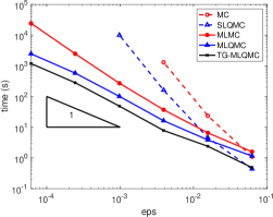
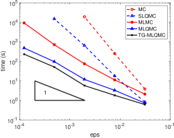
Figure 1: Problem 1: Complexity (measured as time in seconds) of MC, QMC, MLMC, plain-vanilla MLQMC and the enhanced MLQMC method using the two-grid method and nearby QMC points for $\widetilde{p}=4/3$ (left) and $\widetilde{p}=2$ (right).

In Figure 1, we plot the cost, measured as computational time in seconds, against the tolerance $\varepsilon$ for our two MLQMC algorithms, benchmarked against single level MC and QMC, and against MLMC. To ensure an identical bias error for the single- and multilevel methods, the FE meshwidth for the single-level methods is taken to be equal to $h_{L}$, the meshwidth on the finest level of the multilevel methods. The decreasing sequence of tolerances $\varepsilon$ corresponds to a reduction in the finest meshwidth $h_{L}$ by a factor 2 at each step. The axes are in log-log scale, and as a guide the black triangle in the bottom left corner of each plot indicates a slope of $-1$. As expected, the MLQMC algorithms are clearly superior in all cases, and for $\widetilde{p}=2$, the MLMC and single level QMC methods seem to converge at the same rate of approximately $-2$. Also, as we expect the cost of the two MLQMC algorithms grow at the same rate of roughly $-1$, but the enhancements introduced in Algorithm 2 yields a reduction in cost by a (roughly) constant factor of about 2. Note that for this problem the RQ algorithm requires only 3 iterations for almost all cases tested, and so at best we can expect a speedup factor of 3. In almost all of our numerical tests using the eigenvector of a nearby QMC point as the starting vector reduced the number of RQ iterations to 2. A similar speedup by a factor of 2 was also observed in [39], which recycled samples from the multigrid hierarchy within a MLQMC algorithm for the elliptic source problem.

From [19, Corollary 3.1], for our MLQMC algorithms we expect a rate of $-1$ (with a log factor) when $q\leq 2/3$, or equivalently $\widetilde{p}\geq 5/2$. However, we observe for our MLQMC algorithms are close to $-1$, regardless of the decay $\widetilde{p}$. A possible explanation of this is that we use an off-the-shelf lattice rule that hasn’t been tailored to this problem, and so we observe nearly the optimal rate but the constant may still depend on the dimension (which is fixed for these experiments). For the other methods we observe the expected rates, with the exception of QMC, which appears to not yet be in the asymptotic regime. Results for $\widetilde{p}=3$ are very similar to those for $\widetilde{p}=2$, and so have been omitted.

5.2 Problem 2: Domain with interior islands

Consider again the domain $D=(0,1)^{2}$, and the subdomain consisting of four islands given by $D_{\mathrm{f}}\coloneqq[\tfrac{1}{8},\tfrac{3}{8}]^{2}\cup[\tfrac{5}{8},\tfrac{7}{8}]^{2}\cup[\tfrac{1}{8},\tfrac{3}{8}]\times[\tfrac{5}{8},\tfrac{7}{8}]\cup[\tfrac{5}{8},\tfrac{7}{8}]\times[\tfrac{1}{8},\tfrac{3}{8}],$ see Figure 2 for a depiction. Since we use uniform triangular FE meshes with $h_{\ell}=2^{-\ell+3}$ the FE triangulation aligns with the boundaries of the components $D_{\mathrm{f}}$ on all levels $\ell=0,1,2,\ldots$.

Figure 2: Domain $D$ with four islands forming $D_{\mathrm{f}}$ (in grey).

The coefficients are now given by

$$a_{0}({\boldsymbol{x}}) =\begin{cases}\sigma_{\mathrm{diff}}\coloneqq 0.01&\text{if }{\boldsymbol{x}}\in D_{\mathrm{f}},\\[2.84526pt] \sigma_{\mathrm{diff}}^{\prime}\coloneqq 0.011&\text{if }{\boldsymbol{x}}\in D\setminus D_{\mathrm{f}},\end{cases}\quad a_{j}({\boldsymbol{x}})=\begin{cases}\sigma_{\mathrm{diff}}w_{(j+1)/2}(\widetilde{p}_{a};{\boldsymbol{x}})&\text{for $j$ odd},\\[2.84526pt] \sigma_{\mathrm{diff}}^{\prime}w^{\prime}_{j/2}(\widetilde{p}_{a}^{\prime};{\boldsymbol{x}})&\text{for $j$ even},\\ \end{cases}$$

$$b_{0}({\boldsymbol{x}}) =\ \begin{cases}\sigma_{\mathrm{abs}}\coloneqq 2&\text{if }{\boldsymbol{x}}\in D_{\mathrm{f}},\\[2.84526pt] \sigma_{\mathrm{abs}}^{\prime}\coloneqq 0.3&\text{if }{\boldsymbol{x}}\in D\setminus D_{\mathrm{f}},\end{cases}\quad b_{j}({\boldsymbol{x}})=\begin{cases}\sigma_{\mathrm{abs}}w_{(j+1)/2}(\widetilde{p}_{b};{\boldsymbol{x}})&\text{for $j$ odd},\\[2.84526pt] \sigma_{\mathrm{abs}}^{\prime}w^{\prime}_{j/2}(\widetilde{p}_{b}^{\prime};{\boldsymbol{x}})&\text{for $j$ even},\\ \end{cases}$$

where

$$w_{k}(q;{\boldsymbol{x}})\, =\,\begin{cases}\frac{1}{k^{q}}\sin\big{(}8k\pi x_{1}\big{)}\sin\big{(}8(k+1)\pi x_{2}\big{)}&\text{for }{\boldsymbol{x}}\in D_{\mathrm{f}}\,,\\ 0&\text{for }{\boldsymbol{x}}\in D\setminus D_{\mathrm{f}}\,,\text{ and}\end{cases}$$

$$w_{k}^{\prime}(q;{\boldsymbol{x}})\, =\,\begin{cases}0&\text{for }{\boldsymbol{x}}\in D_{\mathrm{f}}\,,\\ \frac{1}{k^{q}}\sin\big{(}8k\pi x_{1}\big{)}\sin\big{(}8(k+1)\pi x_{2}\big{)}&\text{for }{\boldsymbol{x}}\in D\setminus D_{\mathrm{f}}\,,\end{cases}$$

and where the parameters $\widetilde{p}_{a},\widetilde{p}_{a}^{\prime},\widetilde{p}_{b},\widetilde{p}_{b}^{\prime}\geq 4/3$ give the different decays of the coefficients on the different areas of the domain. As for Problem 1, if any of $\widetilde{p}_{a},\widetilde{p}_{a}^{\prime},\widetilde{p}_{b},\widetilde{p}_{b}^{\prime}$ are less than 2, then we scale the corresponding zeroth term in the coefficient by $\pi/\sqrt{2}$.

The complexity of MLMC, MLQMC and the enhanced MLQMC using two-gird methods and nearby QMC points for this problem is given in Figure 3. As expected for both MLQMC algorithms we observe a convergence rate of $-1$, and the MLMC results approach the expected convergence rate of $-2$. Also, since this problem is more difficult for eigensolvers to handle, we now observe that the two-grid MLQMC gives a speedup by a factor of more than 3. Other tests using different values of $\widetilde{p}_{a},\widetilde{p}_{a}^{\prime},\widetilde{p}_{b},\widetilde{p}_{b}^{\prime}$ yielded similar results. Note also that numerical results for single level QMC methods applied to this problem (with slightly different $a_{j}$, $b_{j}$) were given previously in [17].

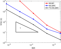
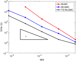
Figure 3: Problem 2: Complexity (measured as time in seconds) of MLMC, plain-vanilla MLQMC and the enhanced MLQMC method using the two-grid method and nearby QMC points for $\widetilde{p}_{a}=\widetilde{p}_{b}=4/3$, $\widetilde{p}_{a}^{\prime}=\widetilde{p}_{b}^{\prime}=2$ (left), and $\widetilde{p}_{a}=\widetilde{p}_{a}^{\prime}=\widetilde{p}_{b}=\widetilde{p}_{b}^{\prime}=2$ (right).

6 Conclusion

We have developed an efficient MLQMC algorithm for random elliptic EVPs, which uses two-grid methods and nearby QMC points to obtain a speedup compared to an ordinary MLQMC implementation. We provided theoretical justification for the use of both strategies. Finally, we presented numerical results for two test problems, which validate the theoretical results from the accompanying paper [19] and also demonstrate the speedup obtained by our new MLQMC algorithm.

Acknowledgements. This work is supported by the Deutsche Forschungsgemeinschaft (German Research Foundation) under Germany’s Excellence Strategy EXC 2181/1 - 390900948 (the Heidelberg STRUCTURES Excellence Cluster). Also, this research includes computations using the computational cluster Katana supported by Research Technology Services at UNSW Sydney.

Appendix A Proof of Theorem 3.1

Proof.

First of all, we can use the triangle inequality to split the eigenfunction error into

$$\|u({\boldsymbol{y}})-u^{h,s}({\boldsymbol{y}})\|_{V}\, \leq\,\|u({\boldsymbol{y}})-u_{s}({\boldsymbol{y}})\|_{V}+\|u_{s}({\boldsymbol{y}})-u_{h,s}({\boldsymbol{y}})\|_{V}+\|u_{h,s}({\boldsymbol{y}})-u^{h,s}({\boldsymbol{y}})\|_{V}$$

$$\lesssim\,h+s^{-(1/p+1)}+\|u_{h,s}({\boldsymbol{y}})-u^{h,s}({\boldsymbol{y}})\|_{V},$$ (A.1)

where we have used [17, Theorem 4.1] and (2.12), and the constant is independent of $h$, $s$ and ${\boldsymbol{y}}$. All that remains for the eigenfunction result is to bound the third term above.

To this end, we can rewrite Step 2 of Algorithm 1 using (3.2) as

$$\mathcal{A}_{s}({\boldsymbol{y}};u^{h,s}({\boldsymbol{y}})-\lambda_{H,S}({\boldsymbol{y}})T_{h,s}u^{h,s}({\boldsymbol{y}}),v_{h})\,=\,\mathcal{A}_{s}({\boldsymbol{y}};T_{h,s}u_{H,S}({\boldsymbol{y}}),v_{h})\quad\text{for all }v_{h}\in V\,,$$

which is equivalent to the operator equation: Find $u^{h,s}({\boldsymbol{y}})\in V_{h}$ such that

$$\bigg{(}\frac{1}{\lambda_{H,S}({\boldsymbol{y}})}-T_{h,s}\bigg{)}u^{h,s}({\boldsymbol{y}})\,=\,\frac{1}{\lambda_{H,S}({\boldsymbol{y}})}T_{h,s}u_{H,S}({\boldsymbol{y}}).$$

This is in turn equivalent (up to a constant scaling factor) to the problem: find $\widetilde{u}\in V_{h}$ such that

$$\bigg{(}\frac{1}{\lambda_{H,S}({\boldsymbol{y}})}-T_{h,s}\bigg{)}\widetilde{u}\,=\,\frac{\lambda_{H,S}({\boldsymbol{y}})T_{h,s}u_{H,S}({\boldsymbol{y}})}{\|\lambda_{H,S}({\boldsymbol{y}})T_{h,s}u_{H,S}({\boldsymbol{y}})\|_{V}}\,\eqqcolon\,u_{0}\,.$$ (A.2)

Explicitly,

$$\widetilde{u}\,=\,\frac{\lambda_{H,S}({\boldsymbol{y}})u^{h,s}({\boldsymbol{y}})}{\|T_{h,s}u_{H,S}({\boldsymbol{y}})\|_{V}},$$

but after normalisation (Step 3) $u^{h,s}({\boldsymbol{y}})=\widetilde{u}/\|\widetilde{u}\|_{\mathcal{M}}$.

We now apply Theorem 3.2 from [47] to (A.2), using the space $X=V$ and with

$$\mu_{0}=\frac{1}{\lambda_{H,S}({\boldsymbol{y}})}\quad\text{and}\quad u_{0}\,=\,\frac{\lambda_{H,S}({\boldsymbol{y}})T_{h,s}u_{H,S}({\boldsymbol{y}})}{\|\lambda_{H,S}({\boldsymbol{y}})T_{h,s}u_{H,S}({\boldsymbol{y}})\|_{V}}.$$

To do so, we must first verify that $\mu_{0}$ and $u_{0}$ satisfy the required assumptions of [47, Theorem 3.2], namely, $\|u_{0}\|_{V}=1$, $\mu_{0}$ is not an eigenvalue of $T_{h,s}$, and for all ${\boldsymbol{y}}\in\Omega$

$$\mathrm{dist}(u_{0},E_{h}(\lambda_{s}({\boldsymbol{y}}))\, \leq\,\frac{1}{2}\quad\text{and}$$ (A.3)

$$|\mu_{0}-\mu_{2,h,s}({\boldsymbol{y}})|\, \geq\,\frac{\mu_{1,s}({\boldsymbol{y}})-\mu_{2,s}({\boldsymbol{y}})}{2}\,\eqqcolon\,\frac{\widetilde{\rho}_{s}({\boldsymbol{y}})}{2}.$$ (A.4)

Recall that $\mu_{k}({\boldsymbol{y}})=1/\lambda_{k}({\boldsymbol{y}})$ is an eigenvalue of $T$, and similarly, subscripts $h$ and $s$ denote their FE and dimension-truncated counterparts, respectively. Clearly, the first two assumptions hold, and so it remains to verify (A.3) and (A.4).

To show (A.3), since $\lambda_{s}({\boldsymbol{y}})$ is simple we have

$$\mathrm{dist}(u_{0}, E_{h}(\lambda_{s}({\boldsymbol{y}}))$$

$$=\,\inf_{\alpha\in\mathbb{R}}\|u_{0}-\alpha u_{h,s}({\boldsymbol{y}})\|_{V}$$

$$=\,\frac{1}{\lambda_{H,S}({\boldsymbol{y}})\|T_{h,s}u_{H,S}({\boldsymbol{y}})\|_{V}}\inf_{\alpha\in\mathbb{R}}\|\lambda_{H,S}({\boldsymbol{y}})T_{h,s}u_{H,S}({\boldsymbol{y}})-\alpha u_{h,s}({\boldsymbol{y}})\|_{V}.$$ (A.5)

To show that the first factor can be bounded by a constant, we use the reverse triangle inequality along with the lower bound (2.15), which since $H>0$ was assumed to be sufficiently small gives

$$\lambda_{H,S}({\boldsymbol{y}})\|T_{h,s}u_{H,S}({\boldsymbol{y}})\|_{V}\,\geq\,\underline{\lambda}\big{|}\|Tu_{H,S}({\boldsymbol{y}})\|_{V}-\|(T-T_{h,s})u_{H,S}({\boldsymbol{y}})\|_{V}\big{|}.$$ (A.6)

Now, by the equivalence of norms (2.5) we have

$$\|Tu_{H,S}({\boldsymbol{y}})\|_{V}\,\geq\,\frac{1}{C_{\mathcal{A}}}\sqrt{\mathcal{A}({\boldsymbol{y}};Tu_{H,S}({\boldsymbol{y}}),Tu_{H,S}({\boldsymbol{y}}))}.$$

Then using the definition of $T$, along with the facts that $u_{H,S}({\boldsymbol{y}})$ is an eigenfunction and $\mathcal{A}({\boldsymbol{y}})$ is symmetric, we can simplify this as

$$\mathcal{A}({\boldsymbol{y}};Tu_{H,S}({\boldsymbol{y}}),Tu_{H,S}({\boldsymbol{y}}))\, =\,\mathcal{M}(u_{H,S}({\boldsymbol{y}}),Tu_{H,S}({\boldsymbol{y}}))$$

$$=\,\frac{1}{\lambda_{H,S}({\boldsymbol{y}})}\mathcal{A}({\boldsymbol{y}};u_{H,S}({\boldsymbol{y}}),Tu_{H,S}({\boldsymbol{y}}))$$

$$=\,\frac{1}{\lambda_{H,S}({\boldsymbol{y}})}\mathcal{M}(u_{H,S}({\boldsymbol{y}}),u_{H,S}({\boldsymbol{y}}))\,\geq\,\frac{1}{\overline{\lambda}},$$

where for the last inequality we have used (2.15) and $\|u_{H,S}({\boldsymbol{y}})\|_{\mathcal{M}}=1$. Hence, we have the constant lower bound

$$\|Tu_{H,S}({\boldsymbol{y}})\|_{V}\,\geq\,C_{\mathcal{A}}^{-1}\overline{\lambda}^{-1/2},$$ (A.7)

which is independent of ${\boldsymbol{y}}$, $S$ and $H$.

For the second term in (A.6), by (3.7) we have the upper bound

$$\|(T-T_{h,s})u_{H,S}({\boldsymbol{y}})\|\, =\,\|T-T_{h,s}\|\|u_{H,S}({\boldsymbol{y}})\|_{V}$$

$$\leq\,C_{T}(s^{-1/p+1}+h)\sqrt{\lambda_{H,S}({\boldsymbol{y}})}\|u_{H,S}({\boldsymbol{y}})\|_{\mathcal{M}}$$

$$\leq\,\overline{\lambda}^{1/2}C_{T}(s^{-1/p+1}+h),$$ (A.8)

where we have used that $u_{H,S}({\boldsymbol{y}})$ is an eigenfunction, normalised in $\mathcal{M}$, and also (2.15).

Returning to (A.6), since $\|Tu_{H,S}({\boldsymbol{y}})\|_{V}$ is bounded from below by a constant, by (A) there exists $S_{0}\in\mathbb{N}$ sufficiently large and $H_{0}>0$ sufficiently small such that for all $s\geq S_{0}$ and $h\leq H_{0}$ we have $\|Tu_{H,S}({\boldsymbol{y}})\|_{V}>\|(T-T_{h,s})u_{H,S}({\boldsymbol{y}})\|_{V}$. Thus, substituting (A.7) and (A) into (A.6), we have the lower bound

$$\lambda_{H,S}({\boldsymbol{y}})\|T_{h,s}u_{H,S}({\boldsymbol{y}})\|_{V}\, \geq\,C_{\mathcal{A}}^{-1}\underline{\lambda}\overline{\lambda}^{-1/2}-\underline{\lambda}\overline{\lambda}^{1/2}C_{T}(s^{-1/p+1}+h)$$

$$\geq\,C_{\mathcal{A}}^{-1}\underline{\lambda}\overline{\lambda}^{-1/2}-\underline{\lambda}\overline{\lambda}^{1/2}C_{T}(S_{0}^{-1/p+1}+H_{0})\,\eqqcolon\,\frac{1}{C_{u_{0}}}\,>\,0,$$

where $0<C_{u_{0}}<\infty$ is independent of $s,S,h,H$ and ${\boldsymbol{y}}$. It follows that

$$\mathrm{dist}\big{(}u_{0},E_{h}(\lambda_{s}({\boldsymbol{y}}))\big{)}\,\leq\,C_{u_{0}}\|u_{h,s}({\boldsymbol{y}})-\lambda_{H,S}({\boldsymbol{y}})T_{h,s}u_{H,S}({\boldsymbol{y}})\|_{V}.$$

For the second factor in (A), using (3.2), for all $v_{h}\in V_{h}$ we have the identity

$$\mathcal{A}_{s}({\boldsymbol{y}};u_{h,s}({\boldsymbol{y}})-\lambda_{H,S}T_{h,s}u_{H,S}({\boldsymbol{y}}),v_{h})\,=\, \big{[}\lambda_{h,s}({\boldsymbol{y}})-\lambda_{H,S}({\boldsymbol{y}})\big{]}\mathcal{M}(u_{H,S}({\boldsymbol{y}}),v_{h})$$

$$+\lambda_{h,s}({\boldsymbol{y}})\mathcal{M}(u_{h,s}({\boldsymbol{y}})-u_{H,S}({\boldsymbol{y}}),v_{h})\,.$$

Letting $v_{h}=u_{h,s}({\boldsymbol{y}})-\lambda_{H,S}({\boldsymbol{y}})T_{h,s}u_{H,S}({\boldsymbol{y}})$, then using that $\mathcal{A}_{s}$ is coercive, as well as applying the triangle and Cauchy–Schwarz inequalities, we have

$$\|u_{h,s}({\boldsymbol{y}})- \lambda_{H,S}T_{h,s}u_{H,S}({\boldsymbol{y}})\|_{V}^{2}$$

$$\lesssim\,\big{|}\lambda_{h,s}({\boldsymbol{y}})-\lambda_{H,S}({\boldsymbol{y}})\big{|}\|u_{H,S}\|_{\mathcal{M}}\|u_{h,s}({\boldsymbol{y}})-\lambda_{H,S}({\boldsymbol{y}})T_{h,s}u_{H,S}({\boldsymbol{y}})\|_{\mathcal{M}}$$

$$\quad+\lambda_{h,s}({\boldsymbol{y}})\|u_{h,s}({\boldsymbol{y}})-u_{H,S}({\boldsymbol{y}})\|_{\mathcal{M}}\|u_{h,s}({\boldsymbol{y}})-\lambda_{H,S}({\boldsymbol{y}})T_{h,s}u_{H,S}({\boldsymbol{y}})\|_{\mathcal{M}}.$$

Dividing through by $\|u_{h,s}({\boldsymbol{y}})-\lambda_{H,S}({\boldsymbol{y}})T_{h,s}u_{H,S}({\boldsymbol{y}})\|_{V}$ and applying the Poincaré inequality (2.7) gives

$$\|u_{h,s}({\boldsymbol{y}})-\lambda_{H,S}T_{h,s}u_{H,S}({\boldsymbol{y}})\|_{V}\\ \,\lesssim\,\big{|}\lambda_{h,s}({\boldsymbol{y}})-\lambda_{H,S}({\boldsymbol{y}})\big{|}+\overline{\lambda}\|u_{h,s}({\boldsymbol{y}})-u_{H,S}({\boldsymbol{y}})\|_{\mathcal{M}},$$

where we have also used that $\|u_{H,S}({\boldsymbol{y}})\|_{\mathcal{M}}=1$ and (2.15). We can incorporate $\overline{\lambda}$ into the constant, and then split the right hand side again using the triangle inequality to give

$$\|u_{h,s}({\boldsymbol{y}})- \lambda_{H,S}T_{h,s}u_{H,S}({\boldsymbol{y}})\|_{V}\,\lesssim\,\big{|}\lambda({\boldsymbol{y}})-\lambda_{s}({\boldsymbol{y}})|+|\lambda_{s}({\boldsymbol{y}})-\lambda_{h,s}({\boldsymbol{y}})|$$

$$+|\lambda({\boldsymbol{y}})-\lambda_{S}({\boldsymbol{y}})|+|\lambda_{S}({\boldsymbol{y}})-\lambda_{H,S}({\boldsymbol{y}})\big{|}+\|u({\boldsymbol{y}})-u_{s}({\boldsymbol{y}})\|_{V}$$

$$+\|u_{s}({\boldsymbol{y}})-u_{h,s}({\boldsymbol{y}})\|_{\mathcal{M}}+\|u({\boldsymbol{y}})-u_{S}({\boldsymbol{y}})\|_{V}+\|u_{S}({\boldsymbol{y}})-u_{H,S}({\boldsymbol{y}})\|_{\mathcal{M}},$$

where we have also applied the Poincaré inequality (2.7) again to switch to the $V$-norms for the eigenfunction truncation errors.

Now, each of the terms in (A) can be bounded by [17, Theorems 2.6 & 4.1] to give

$$\mathrm{dist}(u_{0},E_{h}(\lambda_{s}({\boldsymbol{y}}))\, \lesssim\,\|u_{h,s}({\boldsymbol{y}})-\lambda_{H,S}T_{h,s}u_{H,S}({\boldsymbol{y}})\|_{V}$$

$$\lesssim\,s^{-1/p+1}+S^{-1/p+1}+h^{2}+H^{2},$$ (A.9)

where to bound the FE error in the $\mathcal{M}$-norm we have used [17, eqn. (2.35)] with the functional $\mathcal{G}=\mathcal{M}(\cdot,u_{s}({\boldsymbol{y}})-u_{h,s}({\boldsymbol{y}}))/\|u_{s}({\boldsymbol{y}})-u_{h,s}({\boldsymbol{y}})\|_{\mathcal{M}}\in L^{2}(D)$ (and similarly for $u_{S}({\boldsymbol{y}})-u_{H,S}({\boldsymbol{y}})$). It follows from (A) that there exists $S$ sufficiently large and $H$ sufficiently small — both independent of ${\boldsymbol{y}}$ — such that (A.3) holds.

Next, to verify (A.4), since $\mu_{0}=1/\lambda_{H,S}({\boldsymbol{y}})\eqqcolon\mu_{H,S}({\boldsymbol{y}})$ and since the FE eigenvalues converge from above and thus $\mu_{2,h,s}({\boldsymbol{y}})\leq\mu_{2,s}({\boldsymbol{y}})$,

$$|\mu_{0}-\mu_{2,h,s}({\boldsymbol{y}})|\, =\,\mu_{H,S}({\boldsymbol{y}})-\mu_{2,h,s}({\boldsymbol{y}})\,\geq\,\mu_{H,S}({\boldsymbol{y}})-\mu_{2,s}({\boldsymbol{y}})$$

$$=\,\widetilde{\rho}_{s}({\boldsymbol{y}})-\big{(}\mu_{s}({\boldsymbol{y}})-\mu_{H,S}({\boldsymbol{y}})\big{)}.$$ (A.10)

Now, suppose that $\big{(}\mu_{s}({\boldsymbol{y}})-\mu_{H,S}({\boldsymbol{y}})\big{)}\leq 0$, then (A) simplifies to

$$|\mu_{0}-\mu_{2,h,s}({\boldsymbol{y}})|\,\geq\,\widetilde{\rho}_{s}({\boldsymbol{y}})\,\geq\,\frac{\widetilde{\rho}_{s}({\boldsymbol{y}})}{2},$$

as required. Alternatively, if $\big{(}\mu_{s}({\boldsymbol{y}})-\mu_{H,S}({\boldsymbol{y}})\big{)}>0$ then (A) becomes

$$|\mu_{0}-\mu_{2,h,s}({\boldsymbol{y}})|\,\geq\,\widetilde{\rho}_{s}({\boldsymbol{y}})-\big{|}\mu_{s}({\boldsymbol{y}})-\mu_{H,S}({\boldsymbol{y}})\big{|}.$$

By the triangle inequality we can bound the second term on the right, again using the bounds from [17, Theorems 2.6 & 4.1], as well as (2.15), to give

$$\big{|}\mu_{s}({\boldsymbol{y}})-\mu_{H,S}({\boldsymbol{y}})\big{|}\, \leq\,\frac{|\lambda({\boldsymbol{y}})-\lambda_{s}({\boldsymbol{y}})|}{\lambda({\boldsymbol{y}})\lambda_{s}({\boldsymbol{y}})}+\frac{|\lambda({\boldsymbol{y}})-\lambda_{S}({\boldsymbol{y}})|}{\lambda({\boldsymbol{y}})\lambda_{S}({\boldsymbol{y}})}+\frac{|\lambda_{S}({\boldsymbol{y}})-\lambda_{H,S}({\boldsymbol{y}})|}{\lambda_{S}({\boldsymbol{y}})\lambda_{H,S}({\boldsymbol{y}})}$$

$$\leq\,\frac{C}{\underline{\lambda}^{2}}(s^{-1/p+1}+S^{-1/p+1}+H^{2}).$$

The upper bound is independent of ${\boldsymbol{y}}$, thus we can take $S$ sufficiently large and $H$ sufficiently small, such that, using the bound on the spectral gap in (2.4) together with (2.15),

$$\big{|}\mu_{s}({\boldsymbol{y}})-\mu_{H,S}({\boldsymbol{y}})\big{|}\,\leq\,\frac{1}{2}\frac{\rho}{\overline{\lambda_{1}}\overline{\lambda_{2}}}\,\leq\,\frac{1}{2}\frac{\lambda_{2,s}({\boldsymbol{y}})-\lambda_{s}({\boldsymbol{y}})}{\lambda_{s}({\boldsymbol{y}})\lambda_{2,s}({\boldsymbol{y}})}\,=\,\frac{\widetilde{\rho}_{s}({\boldsymbol{y}})}{2}.$$ (A.11)

Then, to show (A.4) we can substitute the bound above into (A).

Hence, we have verified the assumptions for [47, Theorem 3.2] for all ${\boldsymbol{y}}$. Since $\lambda_{s}({\boldsymbol{y}})$, $\lambda_{h,s}({\boldsymbol{y}})$ are simple, $\mathrm{dist}(u^{h,s}({\boldsymbol{y}}),\widehat{E}_{h}(\lambda_{s}({\boldsymbol{y}}))=\|u_{h,s}({\boldsymbol{y}})-u^{h,s}({\boldsymbol{y}})\|_{V}$ and hence, it now follows from [47, Theorem 3.2] that

$$\|u_{h,s}({\boldsymbol{y}})-u^{h,s}({\boldsymbol{y}})\|_{V}\leq\,\frac{16}{\widetilde{\rho}_{s}({\boldsymbol{y}})}\frac{|\lambda_{h,s}({\boldsymbol{y}})-\lambda_{H,S}({\boldsymbol{y}})|}{\lambda_{h,s}({\boldsymbol{y}})\lambda_{H,S}({\boldsymbol{y}})}\|u_{h,s}({\boldsymbol{y}})-\lambda_{H,S}({\boldsymbol{y}})T_{h,s}u_{H,S}({\boldsymbol{y}})\|_{V}.$$ (A.12)

We handle the three factors in turn. For the first factor, by the argument used in (A.11) we have $1/\widetilde{\rho}_{s}({\boldsymbol{y}})\leq\overline{\lambda_{1}}\overline{\lambda_{2}}/\rho$, independently of ${\boldsymbol{y}}$. For the second factor, we can use the uniform lower bound (2.15), and then the triangle inequality to give the upper bound

$$\frac{|\lambda_{h,s}({\boldsymbol{y}})-\lambda_{H,S}({\boldsymbol{y}})|}{\lambda_{h,s}({\boldsymbol{y}})\lambda_{H,S}({\boldsymbol{y}})}\leq\,\frac{1}{\underline{\lambda}^{2}}\Big{(} |\lambda({\boldsymbol{y}})-\lambda_{s}({\boldsymbol{y}})|+|\lambda_{s}({\boldsymbol{y}})-\lambda_{h,s}({\boldsymbol{y}})|$$

$$+|\lambda({\boldsymbol{y}})-\lambda_{S}({\boldsymbol{y}})|+|\lambda_{S}({\boldsymbol{y}})-\lambda_{H,S}({\boldsymbol{y}})|\Big{)}\,.$$

Each term above can be bounded by using one of Theorems 2.6 or 4.1 from [17] to give

$$\frac{|\lambda_{h,s}({\boldsymbol{y}})-\lambda_{H,S}({\boldsymbol{y}})|}{\lambda_{h,s}({\boldsymbol{y}})\lambda_{H,S}({\boldsymbol{y}})}\,\lesssim\,s^{-(1/p-1)}+h^{2}+S^{-(1/p-1)}+H^{2},$$ (A.13)

where the constant is again independent of $s,S,h,H$ and ${\boldsymbol{y}}$.

Finally, the third factor in (A.12) can be bounded using (A). Hence, substituting (A.13) and (A) into (A.12) we obtain the upper bound

$$\|u_{h,s}({\boldsymbol{y}})-u^{h,s}({\boldsymbol{y}})\|_{V}\, \lesssim\,s^{-2(1/p-1)}+h^{4}+S^{-2(1/p-1)}+H^{4}$$

$$+2\big{(}s^{-(1/p-1)}h^{2}+ s^{-(1/p-1)}S^{-(1/p-1)}+s^{-(1/p-1)}H^{2}+h^{2}S^{-(1/p-1)}+h^{2}H^{2}+S^{-(1/p-1)}H^{2}\big{)}$$

$$\lesssim\,H^{4}+S^{-2(1/p-1)}+H^{2}S^{-(1/p-1)}\,,$$ (A.14)

where we have used the fact that $s\geq S$ and $h\leq H$ to obtain the last inequality. Then to give the error bound (3.8), we simply substitute (A) into (A.1).

The second result (3.9) follows from Lemma 3.1, by choosing $\mathcal{B}=\mathcal{A}({\boldsymbol{y}};\cdot,\cdot)$, $\widetilde{\mathcal{B}}=\mathcal{A}_{s}({\boldsymbol{y}};\cdot,\cdot)=\mathcal{A}({\boldsymbol{y}}_{s};\cdot,\cdot)$, $u=u({\boldsymbol{y}})$ and $w=u^{h,s}({\boldsymbol{y}})$. Noting that $\|u^{h,s}\|_{\mathcal{M}}=1$ and using the definition of $\lambda^{h,s}({\boldsymbol{y}})$ in (3.5), this gives

$$\lambda^{h,s}({\boldsymbol{y}})-\lambda({\boldsymbol{y}})\,=\, \|u({\boldsymbol{y}})-u^{h,s}({\boldsymbol{y}})\|_{\mathcal{A}({\boldsymbol{y}}_{s})}^{2}-\lambda({\boldsymbol{y}})\|u({\boldsymbol{y}})-u^{h,s}({\boldsymbol{y}})\|_{\mathcal{A}({\boldsymbol{y}})}^{2}$$

$$+\mathcal{A}\big{(}{\boldsymbol{y}}-{\boldsymbol{y}}_{s};u({\boldsymbol{y}}),u({\boldsymbol{y}})-2u^{h,s}({\boldsymbol{y}})\big{)}$$

$$\lesssim\, \|u({\boldsymbol{y}})-u^{h,s}({\boldsymbol{y}})\|_{V}^{2}+\mathcal{A}\big{(}{\boldsymbol{y}}-{\boldsymbol{y}}_{s};u({\boldsymbol{y}}),u({\boldsymbol{y}})-2u^{h,s}({\boldsymbol{y}})\big{)},$$ (A.15)

where we simplified using the linearity of $\mathcal{A}({\boldsymbol{y}})$ in ${\boldsymbol{y}}$ and used the equivalence of norms in (2.5) and (2.15), which both hold for all ${\boldsymbol{y}}$.

The last term from (A.15) is bounded as follows

$$\mathcal{A}({\boldsymbol{y}}-{\boldsymbol{y}}_{s}; u({\boldsymbol{y}}),u({\boldsymbol{y}})-2u^{h,s}({\boldsymbol{y}}))$$

$$=\,\int_{D}\sum_{j>s}\big{(}y_{j}a_{j}({\boldsymbol{x}})\nabla u({\boldsymbol{y}})\cdot\nabla[u({\boldsymbol{y}})-2u^{h,s}({\boldsymbol{y}})]$$

$$\qquad\qquad+y_{j}b_{j}({\boldsymbol{x}})u({\boldsymbol{y}})[u({\boldsymbol{y}})-2u^{h,s}({\boldsymbol{y}})]\big{)}\,\mathrm{d}{\boldsymbol{x}}$$

$$\leq\,\frac{1}{2}\sum_{j>s}\big{[}\|a_{j}\|_{L^{\infty}}\|u({\boldsymbol{y}})\|_{V}(\|u({\boldsymbol{y}})\|_{V}+2\|u^{h,s}({\boldsymbol{y}})\|_{V})$$

$$\qquad\qquad+\|b_{j}\|_{L^{\infty}}\|u({\boldsymbol{y}})\|_{L^{2}}(\|u({\boldsymbol{y}})\|_{L^{2}}+2\|u^{h,s}({\boldsymbol{y}})\|_{L^{2}})\big{]}$$

$$\lesssim\,\sum_{j>s}\max\big{(}\|a_{j}\|_{L^{\infty}},\|b_{j}\|_{L^{\infty}}\big{)}\,\lesssim\,s^{-(1/p-1)},$$ (A.16)

where in the second last inequality we have bounded the $V$-norms using (2.16) and the $L^{2}$-norms using the equivalence to the $\mathcal{M}$-norm (2.6), and then used that $u({\boldsymbol{y}})$ and $u^{h,s}({\boldsymbol{y}})$ are normalised. The tail sum in the last inequality is bounded using [33, Theorem 5.1].

Finally, the result (3.9) is obtained by substituting (3.8) and (A.16) into (A.15). ∎

References

• [1] R. Andreev and Ch. Schwab. Sparse tensor approximation of parametric eigenvalue problems. In I. G. Graham et al., editor, Numerical Analysis of Multiscale Problems, Lecture Notes in Computational Science and Engineering, pages 203–241. Springer, Berlin, 2012.
• [2] M. N. Avramova and K. N. Ivanov. Verification, validation and uncertainty quantification in multi-physics modeling for nuclear reactor design and safety analysis. Prog. Nucl. Energy, 52:601––614, 2010.
• [3] D. A. F. Ayres, M. D. Eaton, A. W. Hagues, and M. M. R. Williams. Uncertainty quantification in neutron transport with generalized polynomial chaos using the method of characteristics. Ann. Nucl. Energy, 45:14––28, 2012.
• [4] I. Babuška and J. Osborn. Eigenvalue problems. In P. G. Ciarlet and J. L. Lions, editor, Handbook of Numerical Analysis, Volume 2: Finite Element Methods (Part 1), pages 641–787. Elsevier, Amsterdam, 1991.
• [5] U. Banerjee. A note on the effect of numerical quadrature in finite element eigenvalue approximation. Numer. Math., 61:145–152, 1992.
• [6] A. Barth, Ch. Schwab, and N. Zollinger. Multilevel Monte Carlo finite element method for elliptic PDEs with stochastic coefficients. Numer. Math., 119:123–161, 2011.
• [7] C. Bierig and A. Chernov. Estimation of arbitrary order central statistical moments by the multilevel Monte Carlo method. Stoch. Partial Differ., 4:3–40, 2016.
• [8] K. A. Cliffe, M. B. Giles, R.Scheichl, and A. L. Teckentrup. Multilevel Monte Carlo methods and applications to PDEs with random coefficients. Comput. Visual. Sci., 14:3–15, 2011.
• [9] R. Cools, F.Y. Kuo, and D. Nuyens. Constructing embedded lattices rules for multivariate integration. SIAM J. Sci. Comp., 28:2162–2188, 2006.
• [10] J. Dick, F. Y. Kuo, Q. T. Le Gia, D. Nuyens, and Ch. Schwab. Higher-order QMC Petrov–Galerkin discretization for affine parametric operator equations with random field inputs. SIAM J. Numer. Anal., 52:2676–2702, 2014.
• [11] J. Dick, F. Y. Kuo, and I. H. Sloan. High-dimensional integration: The quasi-Monte Carlo way. Acta Numer., 22:133–288, 2013.
• [12] J. Dick and F. Pillichshammer. Digital Nets and Sequences: Discrepancy Theory and Quasi-Monte Carlo Integration. Cambridge University Press, New York, NY, 2010.
• [13] D. C. Dobson. An efficient method for band structure calculations in 2D photonic crystals. J. Comput. Phys., 149:363–376, 1999.
• [14] J. J. Duderstadt and L. J. Hamilton. Nuclear Reactor Analysis. John Wiley & Sons, New York, NY, 1976.
• [15] H. C. Elman and T. Su. Low-rank solution methods for stochastic eigenvalue problems. SIAM J. Sci. Comp., 41:A2657–A2680, 2019.
• [16] R. Ghanem and D. Ghosh. Efficient characterization of the random eigenvalue problem in a polynomial chaos decomposition. Int. J. Numer. Meth. Engng, 72:486–504, 2007.
• [17] A. D. Gilbert, I. G. Graham, F. Y. Kuo, R. Scheichl, and I. H. Sloan. Analysis of quasi-Monte Carlo methods for elliptic eigenvalue problems with stochastic coefficients. Numer. Math., 142:863–915, 2019.
• [18] A. D. Gilbert, I. G. Graham, R. Scheichl, and I. H. Sloan. Bounding the spectral gap for an elliptic eigenvalue problem with uniformly bounded stochastic coefficients. In D. Wood et al., editor, 2018 MATRIX Annals, pages 29–43. Springer, Cham, 2020.
• [19] A. D. Gilbert and R. Scheichl. Multilevel quasi-Monte Carlo methods for random elliptic eigenvalue problems I: Regularity and analysis. Preprint, arXiv:2010.01044, 2022.
• [20] M. B. Giles. Multilevel Monte Carlo path simulation. Oper. Res., 56:607–617, 2008.
• [21] M. B. Giles and B. Waterhouse. Multilevel quasi-Monte Carlo path simulation. In Advanced Financial Modelling, Radon Series on Computational and Applied Mathematics, pages 165–181. De Gruyter, New York, 2009.
• [22] H. Hakula, V. Kaarnioja, and M. Laaksonen. Approximate methods for stochastic eigenvalue problems. Appl. Math. Comput., 267:664–681, 2015.
• [23] S. Heinrich. Multilevel Monte Carlo methods. In Multigrid Methods, Vol. 2179 of Lecture Notes in Computer Science, pages 58–67. Springer, Berlin, 2001.
• [24] L. Hörmander. The Analysis of Linear Partial Differential Operators I. Springer, Berlin, 2003.
• [25] X. Hu and X. Cheng. Acceleration of a two-grid method for eigenvalue problems. Math. Comp., 80:1287–1301, 2011.
• [26] X. Hu and X. Cheng. Corrigendum to: “Acceleration of a two-grid method for eigenvalue problems”. Math. Comp., 84:2701–2704, 2015.
• [27] E. Jamelota and P. Ciarlet Jr. Fast non-overlapping Schwarz domain decomposition methods for solving the neutron diffusion equation. J. Comput. Phys., 241:445––463, 2013.
• [28] S. Joe. Construction of good rank-1 lattice rules based on the weighted star discrepancy. In H. Niederreiter & D. Talay, editor, Monte Carlo and Quasi-Monte Carlo Methods 2004, pages 181–196. Springer, Berlin, 2006.
• [29] P. Kuchment. The mathematics of photonic crystals. SIAM, Frontiers of Applied Mathematics, 22:207–272, 2001.
• [30] F. Y. Kuo. https://web.maths.unsw.edu.au/~fkuo/lattice/index.html. Accessed August 24, 2020, 2007.
• [31] F. Y. Kuo, R. Scheichl, Ch. Schwab, I. H. Sloan, and E. Ullmann. Multilevel quasi-Monte Carlo methods for lognormal diffusion problems. Math. Comp., 86:2827–2860, 2017.
• [32] F. Y. Kuo, Ch. Schwab, and I. H.Sloan. Multi-level quasi-Monte Carlo finite element methods for a class of elliptic PDEs with random coefficients. Found. Comput. Math, 15:411–449, 2015.
• [33] F. Y. Kuo, Ch. Schwab, and I. H. Sloan. Quasi-Monte Carlo finite element methods for a class of elliptic partial differential equations with random coefficients. SIAM J. Numer. Anal., 50:3351–3374, 2012.
• [34] R. Norton and R. Scheichl. Planewave expansion methods for photonic crystal fibres. Appl. Numer. Math., 63:88–104, 2012.
• [35] D. Nuyens and R. Cools. Fast algorithms for component-by-component construction of rank-1 lattice rules in shift-invariant reproducing kernel Hilbert spaces. Math. Comp., 75:903–920, 2006.
• [36] D. Nuyens and R. Cools. Fast component-by-component construction of rank-1 lattice rules with a non-prime number of points. J. Complexity, 22:4–28, 2006.
• [37] B. N. Parlett. The Symmetric Eigenvalue Problem. Prentice–Hall, Englewood Cliffs, NJ, 1980.
• [38] Z. Qui and Z. Lyu. Vertex combination approach for uncertainty propagation analysis in spacecraft structural system with complex eigenvalue. Acta Astronaut., 171:106–117, 2020.
• [39] P. Robbe, D. Nuyens, and S. Vandewalle. Recycling samples in he multigrid multilevel (quasi)-Monte Carlo method. SIAM J. Sci. Comp., 41:S37–S60, 2019.
• [40] Y. Saad. Numerical Methods for Large Eigenvalue Problems. SIAM, Philadelphia, PA, 2011.
• [41] M. Shinozuka and C. J. Astill. Random eigenvalue problems in structural analysis. AIAA Journal, 10:456–462, 1972.
• [42] I. H. Sloan and H. Woźniakowski. When are quasi-monte carlo algorithms efficient for high dimensional integrals? J. Complexity, 14:1–33, 1998.
• [43] W. T. Thomson. The Theory of Vibration with Applications. Prentice–Hall, Englewood Cliffs, NJ, 1981.
• [44] M. M. R. Williams. A method for solving stochastic eigenvalue problems. Appl. Math. Comput., 215:4729––4744, 2010.
• [45] H. Xie. A multigrid method for eigenvalue problem. J. Comput. Phys., 274:550–561, 2014.
• [46] J. Xu and A. Zhou. A two-grid disretization scheme for eigenvalue problems. Math. Comp., 70:17–25, 1999.
• [47] Y. Yang and H. Bi. Two-grid finite element discretization schemes based on shifted-inverse power method for elliptic eigenvalue problems. SIAM J. Numer. Anal., 49:1602–1624, 2011.