Motif-driven Dense Subgraph Discovery
in Directed and Labeled Networks

Abstract.

Dense regions in networks are an indicator of interesting and unusual information. However, most existing methods only consider simple, undirected, unweighted networks. Complex networks in the real-world often have rich information though: edges are asymmetrical and nodes/edges have categorical and numerical attributes. Finding dense subgraphs in such networks in accordance with this rich information is an important problem with many applications. Furthermore, most existing algorithms ignore the higher-order relationships (i.e., motifs) among the nodes. Motifs are shown to be helpful for dense subgraph discovery but their wide spectrum in heterogeneous networks makes it challenging to utilize them effectively. In this work, we propose quark decomposition framework to locate dense subgraphs that are rich with a given motif. We focus on networks with directed edges and categorical attributes on nodes/edges. For a given motif, our framework builds subgraphs, called quarks, in varying quality and with hierarchical relations. Our framework is versatile, efficient, and extendible. We discuss the limitations and practical instantiations of our framework as well as the role confusion problem that needs to be considered in directed networks. We give an extensive evaluation of our framework in directed, signed-directed, and node-labeled networks. We consider various motifs and evaluate the quark decomposition using several real-world networks. Results show that quark decomposition performs better than the state-of-the-art techniques. Our framework is also practical and scalable to networks with up to 101M edges.

1. Introduction

Dense regions in networks contain unusual and interesting information (Gleich and Seshadhri, 2012). Dense subgraph discovery is shown to be an effective analysis method in many applications across various domains (Lee et al., 2010; Kumar et al., 1999; Alvarez-Hamelin et al., 2006; Fratkin et al., 2006; Du et al., 2009; Jin et al., 2009; Gionis et al., 2013). It is often a good and cheaper proxy for graph clustering because cohesive subgraphs in real-world networks exhibit good cuts (Lee et al., 2010; Gleich and Seshadhri, 2012). However, most algorithms to find dense subgraphs are designed for simple, undirected, unweighted graphs. In reality, a common characteristic of natural and engineered systems from various domains is that the nodes (entities) and edges (relationships) have rich information associated with them; i.e., networks are heterogeneous (Sun and Han, 2012). Relationships can be asymmetrical (one-way) and entities/relationships can be associated with categorical and numerical attributes; e.g., length of a road or gender of a person. Finding the dense subgraphs while actively considering the rich information on nodes/edges has various applications, such as entity resolution (Wang et al., 2016) and link prediction (Carranza et al., 2020).

Furthermore, most dense subgraph discovery algorithms are designed to capture only the first-order relationships. Higher-order structures (i.e., motifs/graphlets) are shown to be the fundamental building blocks in the organization and dynamics of real-world networks such as social and neural networks (Milo et al., 2002; Pržulj, 2007; Seshadhri et al., 2014; Pinar et al., 2017; Ahmed et al., 2016; Jain and Seshadhri, 2017). Discovering dense subgraphs that have a higher-order structure is imperative in the analysis of those networks. In simple networks, motifs are used to find subgraphs with higher-order structure, which cannot be detected with edge-centric methods (Tsourakakis, 2015; Sarıyüce et al., 2015). However, it is not clear how to find dense subgraphs with motifs in heterogeneous networks. The spectrum of motifs in heterogeneous networks is wide due to the edge directions and node/edge attributes. Although this variety is particularly effective for the analysis as the structure and dynamics can vary with respect to the type of motif considered (Benson et al., 2016; Tsourakakis et al., 2017; Sun et al., 2011), handling the diverse nature of heterogeneous networks while watching for the motifs is a challenging problem.

In this work, we introduce the quark decomposition framework to find motif-driven subgraphs in networks with directed edges and categorical attributes on nodes/edges. Our framework builds subgraphs, called quarks, in varying quality and with hierarchical relations. A $k$-quark is a motif-parameterized subgraph where each node/edge (or small motif) participates in a number of (larger) motifs. The parameter $k$ denotes the extent of participation and not an input: quark decomposition finds non-empty $k$-quarks for all $k$ values. Our framework is inspired by the peeling approach in simple graphs, namely core, truss, and nucleus decompositions (Seidman, 1983; Cohen, 2008; Sarıyüce et al., 2015), which first locate the outer sparse parts of the graph and then find the inner dense regions. Given the practicality and effectiveness of the peeling techniques, we adapt them to the directed networks with categorical attributes in a principled way. Note that it is beyond nontrivial to consider a generalization since edge directions and node/edge attributes create a wide and diverse spectrum of motifs (see Figure 1 and Figure 6 for examples).

Quark decomposition takes two motifs as parameters, $M$ and $N$ where $M\subset N$, and builds subgraphs where $M$s participate in many $N$s. The parameterized formulation enables the discovery of diverse subgraphs and lets a trade-off between quality and practicality. We assign density indicators for each motif $M$, called quark numbers, to denote how well $M$ is connected to its neighborhood, which are then used to build the $k$-quarks. Quark numbers also relate the $k$-quarks with each other using containment relations; the quarks with larger $k$ are contained in the ones with smaller $k$.

We use quark decomposition in two broad classes of applications: (1) When the motif of interest is unknown and higher-order organization of the network is asked; (2) When the motif of interest is known and guides the quark decomposition. For (1), we compare quarks obtained with various motifs and analyze the number and quality of resulting quarks in directed and signed-directed networks. In a word-association network, we show that overlapping quarks by the same motif as well as the quarks by different motifs capture diverse contexts of the words. We also analyze the Florida Bay food web and show that quarks obtain consistently better results than the state-of-the-art algorithm for finding groups of compartments with respect to the ground-truth classifications. For (2), we consider the task of finding gender-balanced communities in networks where genders are used as node labels. We focus on the college friendship networks that have low female ratios. We consider clique-based instantiations of the quark decomposition and choose gender-balanced triangles and four-cliques as the motif $N$. We observe consistently high female ratios when compared to the label-oblivious state-of-the-art methods.

Key contributions in this paper are summarized as follows:

• Quark decomposition. We propose a framework to find dense subgraphs according to a given motif in networks with directed edges and categorical attributes on nodes/edges. Quark decomposition is versatile, efficient, and extendible.

• Limitations and role confusion problem. We characterize the limitations and practical instantiations of quark decomposition to guide the selection of parameter motifs $M$ and $N$. Presence of multiple orbits in some directed motifs results in subgraphs where a node/edge serves in multiple orbits. We call this role confusion and devise role-aware quark numbers as a remedy.

• Generic peeling algorithm for any motif. We introduce a generic peeling algorithm that works for any motif pair $M,N$ to find the quark decomposition. Our algorithm is similar in spirit to the core/truss/nucleus decompositions and can enjoy the optimizations applicable for the peeling algorithms.

• Extensive evaluation on real-world networks. We evaluate quark decomposition on three types of heterogeneous networks; directed, signed-directed, and node-labeled. We consider various motifs using several real-world networks. Results show that quark decomposition outperforms the state-of-the-art techniques and is also practically scalable to networks with up to 101M edges.

2. Related Work

Here we summarize the related works on motif-driven dense subgraphs in heterogeneous networks. Note that there are too many clustering, community detection/search works on heterogeneous networks (Fang et al., 2020), but our focus is limited to motif-based approaches that find dense subgraphs in directed and labeled networks.

Peeling approaches on simple networks. Core decomposition is a simple but effective model to locate the seed regions where dense subgraphs can be found (Seidman, 1983). It makes use of degrees to assign core numbers to nodes. Regularizing the node degrees, that span to a large range, to the core numbers in a smaller range is the key and makes the peeling a fundamental building block in an array of applications (Peng et al., 2014; Kitsak et al., 2010; Malliaros et al., 2016; Alvarez-Hamelin et al., 2006; Carmi et al., 2007). Higher-order variants of the peeling are introduced to take advantage of the triangles and small subgraphs. Truss decomposition leverages triangles (Saito and Yamada, 2006; Cohen, 2008; Huang et al., 2014), nucleus decomposition makes use of small cliques (Sarıyüce et al., 2015; Sariyüce et al., 2017), and tip/wing decomposition utilizes butterflies ($2,2$-bicliques) in bipartite networks (Aksoy et al., 2017; Sariyüce and Pinar, 2018) to find dense regions in a principled way. Nucleus decomposition generalizes core and truss decompositions. It finds $k$-$(r,s)$ nucleus, defined as a subgraph where each $r$-clique is a part of $k$ number of $s$-cliques where $r<s$. Those peeling approaches work on undirected simple networks. Here we work on directed networks with attributes on nodes/edges. We compare our methods with nucleus decomposition to highlight the benefit of considering edge directions and node labels.

Cycle-, flow-trusses. Regarding the adaptations of core and truss decompositions for directed graphs, Takaguchi and Yoshida (Takaguchi and Yoshida, 2016) introduced cycle- and flow-trusses. Their algorithms work on directed networks with respect to cycle and flow (acyclic) motifs (see Figure 1) and rely on the occurrences of the cycle and flow motifs for each edge. However, they do not consider the bidirectional edges and handle each such edge as two separate unidirectional edges. We compare our work with cycle-flow trusses in Section 5.1.

Motif-based densest subgraph and clique finding. There are a few works in the literature that studies the motif-driven densest subgraph problem. For constant size cliques, which can be thought of as motifs in simple undirected graphs, Tsourakakis introduced the $k$-clique densest subgraph problem (Tsourakakis, 2015) to generalize the classical densest subgraph discovery (Goldberg, 1984) for $k$-cliques ($k>2$). Analogous to finding the subgraph with the maximum average degree, Tsourakakis proposed to find the subgraphs that have a maximum average triangle (or $k$-clique) count per node. More recently, Fang et al. proposed exact and approximate algorithms for the same problem (Fang et al., 2019) and Hu et al. considered heterogeneous information networks with specific schemas to find maximal motif-cliques (Hu et al., 2019). Note that our problem setup is more general and we aim to find multiple subgraphs that are not necessarily perfect cliques but always significantly dense.

Higher-order motif clustering. The motif-based graph clustering problem is studied from a spectral perspective in heterogeneous networks. Benson et al. (Benson et al., 2016) introduced a nice generalized framework for clustering the networks based on the higher-order connectivity patterns. They defined the motif conductance as the ratio of the number of motifs cutting the border between two regions to the number of motif instance endpoints (i.e., nodes) in the subgraph or its complement, whichever is smaller. Since getting the optimal solution for motif conductance is NP-Hard, they proposed an approximate algorithm that finds the near-optimal cluster in a given network. Their method relies on the spectral clustering of motif adjacency matrix whose entry $i,j$ is the number of motifs where nodes $i$ and $j$ co-occur. The set of nodes in the spectral ordering that has the minimum conductance is reported as the optimal higher-order cluster. Recursive bisection method iteratively finds the near-optimal clusters in the complement of the graph and k-means clustering on the motif adjacency matrix obtains a prespecified number of clusters. Concurrently, Tsourakakis et al. (Tsourakakis et al., 2017) proposed the same framework for motif-aware clustering and also introduced a random walk interpretation of the graph reweighting scheme which gives a principled approach to define the notion of conductance for other motifs. More recently, Li et al. improved the motif-based clustering approach to handle the clustering of disconnected nodes (Li et al., 2019). Our framework differs from those approaches: we do not partition the graph but find dense subgraphs around nodes/edges. We give an extensive comparison against the motif clustering (Benson et al., 2016) in our experiments.

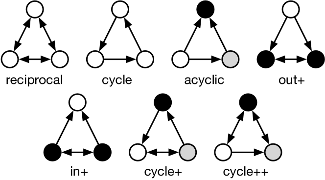
Figure 1. Directed triangle motifs with three nodes and three edges, as named in (Seshadhri et al., 2016). Automorphism orbit (or just orbit) of a node in a given motif is the set of other nodes that have the same topological connectivity patterns. In each triangle, orbits of the nodes are denoted with colors (i.e., nodes in the same color have the same orbit).

3. Preliminaries

Motifs and hypergraphs. We define motif $M=(V_{M},E_{M})$ as an induced directed subgraph with node and edge sets $V_{M}$, $E_{M}$. Each $v\in V_{M}$ and $e\in E_{M}$ can have categorical (non-numeric) attributes, defined by $f:V_{M},E_{M}\rightarrow\mathcal{N}$. A motif $M$ is a subset of motif $N$ iff

• $V_{M}\subseteq V_{N}$ where there is one and only one $v^{\prime}\in V_{N}$ for each $v\in V_{M}$ such that $f(v)=f(v^{\prime})$.

• $E_{M}\subseteq E_{N}$ where there is one and only one $e^{\prime}\in E_{N}$ for each $e\in E_{M}$ such that $f(e)=f(e^{\prime})$.

We use the language of hypergraphs to define the involvements of small motifs in the larger motifs. A hypergraph $H=(V,E)$ consists of the node set $V$ and hyperedge set $E$, where a hyperedge $e\in E$ is simply a subset of $V$ (in standard graphs, each hyperedge has two nodes). Consider a hypergraph $H=(V,E)$;

• $u,v\in V$ are neighbors if there is a hyperedge $e\in E$ that contains $u$ and $v$.

• The degree of a node $v\in V$, denoted by $d(v)$, is the number of hyperedges that contain $v$.

• The size of a hyperedge $e\in E$, denoted by $s(e)$, is the number of nodes in it.

• Two nodes $u$ and $v$ are connected if there exists a sequence of hyperedges $e_{1},e_{2},\ldots,e_{\ell}\in E$ such that $u\in e_{1}$, $v\in e_{\ell}$, and $\forall i<\ell$, $e_{i}\cap e_{i+1}\neq\emptyset$.

• $H$ is connected if all pairs of nodes are connected.

Definition 0.

Let $S\subseteq V$. The induced hypergraph $H|_{S}$ has node set $S$ and contains every hyperedge of $H$ completely contained in $S$, i.e., $\forall e\in H|_{S}$, iff $v\in e$ then $v\in S$.

• The degree of node $v$ $\in$ $H|_{S}$ is denoted by $d_{S}(v)$ (or $d(v)$ when clear).

• The minimum degree in $H|_{S}$ is denoted by $\delta_{S}$.

Induced hypergraph is also known as section hypergraph.

Dense subgraphs. We call a subgraph dense if it has many motifs (also called motif-based or -driven dense subgraph). Formally, we use average motif degree to quantify the density of a subgraph with respect to a given motif.

Definition 0.

For a subgraph $S$ and a motif $N$, the average motif degree of $S$ is the number of instances of $N$ in $S$ divided by the number of nodes in $S$.

4. Quark decomposition framework

We first define the motif hypergraph.

Definition 0.

Given a graph $G$ and template motifs $M$ and $N$ s.t. $M\subset N$. Let $\{M\}$ and $\{N\}$ be the set of instances of $M$ and $N$ in $G$, respectively, and $f,g$ be bijective functions. Motif hypergraph $H_{G}(M,N)=(V_{G},E_{G})$ is a hypergraph constructed as follows:

• Each instance of $M\in G$ forms a node $u\in V_{G}$ by $f$:$\{M\}\rightarrow{V_{G}}$.

• Each instance of $N\in G$ forms a hyperedge $e\in E_{G}$ by $g$:$\{N\}\rightarrow{E_{G}}$.

• Iff $M\subset N$ in $G$, then $f(M)\in g(N)$ in $H_{G}$.

Note that $H_{G}(M,N)$ is a $t$-uniform hypergraph (i.e., $s(e)=t~{}~{}\forall e\in E_{G}$) where $t$ is the number of occurrences of $M$ in $N$. We also refer to the degree of each node $u\in H_{G}$ as the motif degree, denoted by $d_{H_{G}}(u)$ (or $d(u)$ when $H_{G}$ is obvious).

We now introduce the notion of k-quark subgraph.

Definition 0.

Given a graph $G$ and template motifs $M$, $N$ such that $M\subset N$, say $H_{G}(M,N)$ is the motif hypergraph defined as above.

• For any $k\in\mathbb{N}$, a k -quark of $H_{G}(M,N)$ is a connected and maximal induced sub-hypergraph $H|_{S}$ such that $\delta_{S}\geq k$.

• For a node $u$ in $H_{G}(M,N)$ (corresponding to an instance of motif $M$ in $G$), the quark number of $u$, denoted by ${\mathcal{K}({u})}$, is the largest value of $k$ such that $u$ belongs to a non-empty $k$-quark.

We also refer to $k$-quark as quark when $k$ is irrelevant or clear.

Definition 0.

$k$-quarks form a hierarchy by containment.

• Let $S$ be a $k$-quark and $T$ be a $k^{\prime}$-quark such that $k^{\prime}<k$ and $S\subset T$. $S$ is the child of $T$ (and $T$ is the parent of $S$) if there is no $\bar{k}$-quark $U$ such that $k^{\prime}<\bar{k}<k$ and $S\subset U\subset T$.

• A $k$-quark is leaf (childless) if there is no $k^{+}$-quark in it s.t. $k^{+}>k$.

• Maximum quark number of a graph is the largest $k$ for which there is a non-empty $k$-quark.

• Maximum $k$-quark is a quark where $k$ is the maximum quark number in the graph.

Quark decomposition is the process of finding the quark numbers and $k$-quarks for a given pair of motifs $M,N$ in a graph $G$. Leaf $k$-quarks are the locally optimal subgraphs; they are surrounded by less dense quarks (with lower $k$ values) and hence often contain the most interesting information.

If $G$ is a simple undirected graph where $M$ is $r$-clique and $N$ is $s$-clique ($r<s$), then $k$-quark is nothing but a $k$-$(r,s)$ nucleus (Sarıyüce et al., 2015; Sariyüce et al., 2017). If $G$ is a simple undirected bipartite graph where $M$ is edge and $N$ is $2,2$-biclique, then $k$-quark reduces to be a $k$-wing (Sariyüce and Pinar, 2018). In the quark decomposition, each $M$ instance is given a quark number and the $k$-quarks along with the hierarchical relationships among them can be constructed accordingly. Note that, $N$ is the motif of interest for which dense regions are to be found. Motif $M$ can be any subset of $N$ but it should satisfy some requirements such that non-trivial $k$-quarks can be obtained (more details given in Section 4.1). When $M$ is edge or a larger motif, the resulting $k$-quarks may overlap with each other because quarks are defined as a group of $M$s. This is useful since the overlapping communities can better capture the network organization (Xie et al., 2013).

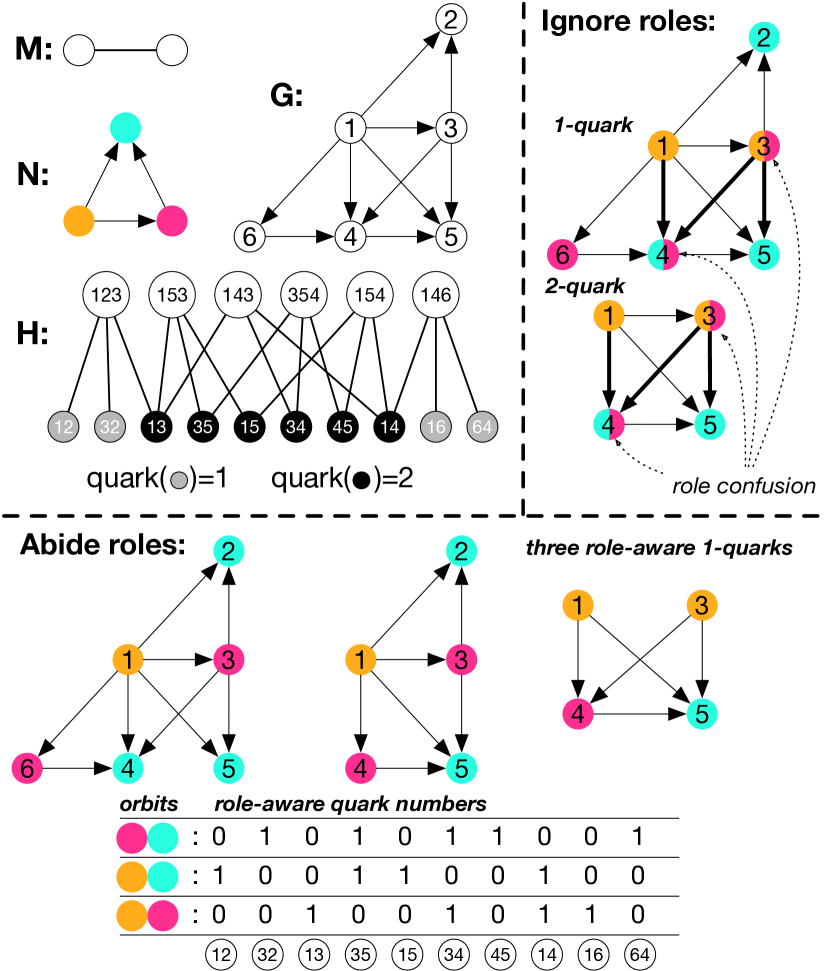
Figure 2. We construct the motif hypergraph H  with respect to the motifs M  (edge) and N  (acyclic) on a toy graph G  (in top-left). Each orbit in N  is shown by a different color. We create a node for each motif M  and a hyperedge for each motif N  to get the motif hypergraph H . Ids of triangles and edges are the union of the nodes in each. Quark numbers are denoted with gray for 1 and black for 2. 1-quark and 2-quark are shown in top-right. Role confusion occurs for nodes 3 and 4 in both quarks. Role-aware quarks and quark numbers are shown at the bottom (See Section 4.1.2 for more details).

4.1. Limitations & practical instantiations

It is important to consider the necessary and sufficient conditions for the $M$ and $N$ in Definition 2 so that the $k$-quarks are non-trivial. For instance, if $M$ has only one occurrence in $N$, the size of each hyperedge in the motif hypergraph becomes one, thus it is not possible to consider any connectivity among $M$s. This is related to the automorphism orbits (Pržulj, 2007; Sarajlić et al., 2016). Automorphism orbit (or just orbit) of a node in a given motif is the set of other nodes that have the same topological connectivity patterns. For directed triangle motifs, shown in Figure 1, orbits of the nodes are denoted with colors. For instance, in+ has two orbits; the first has one node with two incoming edges (white node) and the second has two nodes where each has one outgoing and one bidirectional edge (black nodes). Note that automorphism orbits are defined only for the nodes. In our framework, we can also consider an edge or a larger structure as $M$ in Definition 2, thus automorphism orbits of such structures need to be taken into account. To define the orbits of any $M$, we consider the ordered list of node orbits in it.

Enforcing the automorphism orbits restricts the use of any motif since Definition 2 requires that at least one orbit should have multiple instances in $N$. E.g., when $M$ is node or edge; acyclic, cycle+, and cycle++ motifs have three different orbits, i.e., no orbit has multiple members. Thus those cannot be considered as $N$. To remedy this problem, we use a vanilla motif $M$, which has only one orbit. A vanilla motif has no node/edge labels and its edges are directionless. Any motif $N\supset M$ will contain multiple instances of $M$, thus the size of hyperedges will be greater than one. Figure 2 gives an example when $M$ is a vanilla edge and $N$ is acyclic.

4.1.1. Role confusion problem

Another problem in $k$-quarks is the conflation of the orbits for $M$s. An instance of $M$ can be a part of multiple instances of $N$. Furthermore, orbit of an $M$ instance in one $N$ instance can be different than its orbit in another $N$ instance. E.g., if $M$ is node and $N$ is out+, a node may appear as white node in one out+ instance while being black node in another out+ instance (see Figure 1). We call this the role confusion problem. Note that choosing $M$ as a vanilla motif does not help with the role confusion problem. For example, consider cycle+ with nodes $A,B,C$ and edges $A$$\rightarrow$$B$, $B$$\rightarrow$$C$, $A$$\leftrightarrow$$C$. This can be a structure in Twitter network; e.g., A is a grad student, C is her advisor (a professor), and B is a junior faculty working in the same field—B is an interesting person for A but not for C, professor C is a well-known person followed by many and she follows A since she is A’s advisor. In the motif-driven subgraphs for cycle+, each node has ideally a single role; i.e., a grad student is better characterized as the node A in all the cycle+ instances she participates in. The solution is to construct the subgraphs in a way that abide by the orbits. To do that, we define role-aware quark numbers for each $M$. If $M$ has $b$ orbits in $N$, each $M$ will have $b$ role-aware quark numbers, one for each orbit.

Definition 0.

Given a graph $G$ and motifs (vanilla) $M$ and $N$ (s.t. $M\subset N$), let $H_{G}(M,N)$ be the motif hypergraph as defined in Definition 1. Let $b$ be the number of orbits of $M$ in $N$.

• Orbit degree of an $M$ instance is the number of instances of $N$ that contain it such that the orbit of the $M$ instance in each $N$ instance is the same. Each $M$ instance has $b$ orbit degrees.

• For any $k\in\mathbb{N}$, a role-aware k -quark of $H_{G}(M,N)$ is a connected and maximal induced sub-hypergraph $H|_{S}$ such that each $M$ instance has one orbit degree of at least $k$.

• For a node $u$ in $H_{G}(M,N)$ (corresponding to an instance of motif $M$ in $G$), the role-aware quark numbers of $u$ are $b$ numbers, denoted by ${\mathcal{K}_{i}({u})}$ for $1\leq i\leq b$. ${\mathcal{K}_{i}({u})}$ is the largest value of $k$ such that the node $u$ belongs to a non-empty role-aware $k$-quark where its orbit is $i$.

In a role-aware $k$-quark, each $M$ instance participates in at least $k$ $N$ instances and the orbit of the $M$ instance in each of those participations is the same (note that different $M$ instances can have different orbits in the quark). Role-aware quark numbers describe the extent of participation as a particular orbit while the quark number indicates the extent of participation as any orbit. When $M$ is node and $N$ is cycle or reciprocal (in Figure 1), there is no role confusion since there is only one node orbit in each. For all the other directed triangles, there is a role confusion. When $M$ is edge, we always consider the orbits of the two nodes in it. In the context of directed triangles, one important point is the distinction between unidirectional and bidirectional edges. In this work, we consider the bidirectional edge as an atomic entity; i.e., not combination of two unidirectional edges, due to the fact that a symmetrical relation has a different semantic than two asymmetrical ones—in a sense we only consider the induced edges. For instance, in+ and out+ do not create any role confusion when $M$ is edge, because the unidirectional edge between the white and black nodes in in+ (or out+) cannot serve as a bidirectional edge (between two black nodes) in an adjacent in+ (or out+) motif (see Figure 1).

4.1.2. Example

Figure 2 illustrates an example on a toy graph. We choose the vanilla edge as the motif $M$ and acyclic triangle as the motif $N$, shown in the top-left. We denote the node orbits in acyclic with different colors; orange shows the node with two outgoing edges, blue is for the node with two incoming edges, and red denotes the node with one incoming and one outgoing edge. Motif hypergraph, $H$, with respect to $G,M,N$ is shown next. As described in Definition 1, we create a node for each vanilla edge (bottom set in $H$) and a hyperedge for each acyclic (top set in $H$). Id of each acyclic and edge in $H$ is formed by the concatenation of the node ids in it, e.g., $12$ denotes the edge from $1$ to $2$. Each hyperedge is connected to three nodes since there are three edges in an acyclic—making $H$ a $3$-uniform hypergraph. The degree of each node in $H$ is called the motif degree, e.g., it is $2$ for edge $4$-$5$. Quark numbers of the edges are denoted by gray ($\mathcal{K}=1$) and black ($\mathcal{K}=2$) in the bottom set of $H$; e.g., quark number of edge $4$-$5$ is $2$. Based on those quark numbers, we construct the quarks in the top-right. Two quarks are created; a $1$-quark, corresponding to the entire graph $G$, and a $2$-quark with nodes $1,3,4,$ and $5$. We observe role confusions for the thick edges in those quarks, which in turn implies the role confusions on nodes. Regarding the edges, $1$-$4$, $3$-$4$, and $3$-$5$ have role confusion in both quarks; e.g., in 1-quark, $1$-$4$ connects orange to blue in $1$-$4$-$6$ acyclic but it links orange to red in $1$-$5$-$4$ acyclic. For the nodes, $3$ and $4$ in both quarks have role confusions, e.g., node $3$ is red in the $1$-$3$-$5$ acyclic (and in $1$-$3$-$4$) while being orange in the $3$-$4$-$5$ acyclic. We give the role-aware quarks and quark numbers of the edges at the bottom. If we construct the role-aware quarks by abiding the orbits, we get three role-aware 1-quarks. Note that the only edges that have multiple non-zero $\mathcal{K}_{i}$ are the ones that have role confusion in the top-right.

4.2. Algorithms

Here we discuss our peeling algorithms, first for quark decomposition (Definition 2) and then for role-aware quarks (Definition 4).

4.2.1. Quark decomposition

Algorithm 1 outlines the quark decomposition. Here we assume the motif $M$ in Definition 2 to be node or edge for simplicity. Note that larger structures can be considered as well. Also, we avoid constructing the actual hypergraph of motifs since it requires enumerating all the $N$s which will have a significant space cost. Instead, we discover those motifs for each node/edge as needed, similar to the space-efficient approach in nucleus decomposition (Sarıyüce et al., 2015). There are three different phases in the quark decomposition; motif degree counting, peeling to find quark numbers, and constructing the subgraphs and the hierarchy.

Motif degree counting. Line 1 corresponds to counting the occurrences of $N$ instances per each node or edge. There are some studies (Melckenbeeck et al., 2018; Pinar et al., 2017; Yaveroğlu et al., 2014) that leverage certain commonalities among motifs to avoid redundant computations. Adapting those studies for per node/edge motif counting to improve runtime is possible but out of scope for this work. Also, simultaneously counting the motif degrees for multiple motifs would speed up the workflow when the motif of interest is unknown to the user and multiple options need to be investigated. Note that if the label set of the input motif $N$ is smaller than the label set of the input graph $G$, we can filter the graph to only keep the label set of $N$, e.g., if a triangle of female students is $N$ for an undirected graph where genders are the node labels, only the induced graph of female nodes can be considered.

Peeling to find quark numbers. Lines 1 to 1 assigns a quark number for each node/edge. The classical core decomposition implementation (Batagelj and Zaversnik, 2003) makes use of the bucket data structure to keep track of the nodes with the minimum degree. We also use this approach to watch the nodes/edges with the minimum motif degree. Initially, all the nodes/edges are marked as unprocessed (line 1), which will come handy to ensure each $N$ instance is processed only once. In each iteration, an unprocessed node/edge with the minimum motif degree is chosen (line 1). The motif degree of the chosen node/edge is set to be its quark number ($\mathcal{K}$) (line 1). Then, the $N$ instances that contain the chosen node/edge are found and processed in lines 1 to 1. In each such instance of $N$, we make sure that the other nodes/edges (the neighbors of the chosen node/edge) are unprocessed (line 1); this is done to ensure that each $N$ instance is examined only once. Then, the neighbor nodes/edges in each $N$ instance are checked (line 1) and their motif degree is decremented if larger than the motif degree of the chosen node/edge (lines 1 and 1). At the end of the iteration, the chosen node/edge is marked as processed (line 1). For any $M,N$ motif pair, two basic procedures are necessary and sufficient to instantiate the quark decomposition;

• Finding the $N$ instances that contain a given $M$ instance (line 1),

• Finding the $M$ instances in a given $N$ instance (lines 1 and 1).

Constructing the subgraphs and the hierarchy. It is also possible to construct the subgraphs and build hierarchy among $k$-quarks during the peeling operation, as noted in magenta lines after lines 1 and 1. Subgraph and hierarchy construction during the peeling process is introduced in (Sariyüce and Pinar, 2016) and can be adapted to the quark decomposition. In line 1, the nodes/edges that are in the same $N$ instance with the chosen node/edge are checked. If those nodes/edges are already processed (i.e., assigned a quark number), we can build non-maximal $k$-quarks during the peeling process. At the end, those non-maximal $k$-quarks are converted to the real (maximal) $k$-quarks with a light-weight post-processing that uses the union-find data structure (following line 1).

Compute $d(u)$ (motif deg.) $\forall~{}u\in V$  // or $d(e)$ $\forall~{}e\in E$

1 Mark every $u$ (or $e$) as unprocessed

2 for each unprocessed $u$ (or $e$) with minimum degree $d$ do

      $\mathcal{K}(u)\leftarrow d(u)$ // or $\mathcal{K}(e)\leftarrow d(e)$

3      for each motif $N$ s.t.  $u\subset N$ (or $e\subset N$) do

4           if any node $v\in N$ is processed (or edge) then continue

           // can also find subgraphs & hierarchy

5           for each node $v~{}(\neq u)\subset N$ (or edge $f~{}(\neq e)$) do

6                if $d(v)>d(u)$ (or $d(f)>d(e)$) then

                     $d(v)\leftarrow d(v)-1$ // or $d(f)\leftarrow d(f)-1$

7                    

8                    

9                    

10                     Mark $u$ (or $e$) as processed

11                    

                     // Optional post-processing to build the hierarchy

12                     return array $\mathcal{K}(\cdot)$

Algorithm 1 Quark Decomposition ($G\,(V,E)$, motif $N$)

Theorem 5.

Given a graph $G=(V,E)$ and motif $N$, Algorithm 1 finds the quark numbers, ${\mathcal{K}({\cdot})}$, of all $u\in V$ (or $e\in E$).

Proof.

We give the proof for the node case without loss of generality (i.e., it is similar for the edge). As noted in Section 3, nodes $u,v\in V$ are neighbors if they participate in a common motif $N$. ${\mathcal{K}({u})}=k$ indicates that there are at least $k$ instances of $N$ which contain $u$ and in each such $N$, $u$ has a neighbor node $v$ s.t. ${\mathcal{K}({v})}\geq{\mathcal{K}({u})}$. This is enforced by the lines 1-1, where the motif degree a neighbor node is decreased if it is larger than the quark number assigned at that step. In other words, any neighbor node with a smaller quark number does not contribute to the quark number of the node of interest. If Algorithm 1 finds ${\mathcal{K}({u})}=k$ for a node $u\in V$, then by Definition 2, we need to show that (i) $\exists$ a $k$-quark $G^{\prime}\ni u$, (ii) $\nexists$ a $k^{+}$-quark $G^{\prime}\ni u$ ($k^{+}>k$).
(i) Once ${\mathcal{K}({u})}=k$ is found in Algorithm 1, we stop and construct an induced subgraph $G^{\prime}\subset G$ by traversal as follows. Initially, $G^{\prime}$ has only $u$. In each step, we visit a node $v\in V$ s.t. $v$ co-participates in some $N$ instance with a node from $G^{\prime}$. If ${\mathcal{K}({v})}=k$ or if it is unassigned but its current motif degree is equal to $k$, we add $v$ to $G^{\prime}$. We continue the traversal until no such node $v$ can be found. At the end, $G^{\prime}$ is a $k$-quark since (1) each node participates in $\geq k$ motifs, because the nodes are processed in the non-decreasing order of their motif degrees, (2) all the nodes are connected to each other with motifs due to the motif-based traversal, and (3) $G^{\prime}$ is maximal since it is the largest subgraph that can be found by the traversal.
(ii) $u$ cannot be in a $k^{+}$-quark. Assume it is. Then it should take part in at least $k^{+}$ motifs and each motif contains a neighbor node with motif degree of at least $k^{+}$. But, this implies that ${\mathcal{K}({u})}=k^{+}$ (by Definition 2), contradiction. ∎

Time and space complexity. Algorithm 1 has $O(\sum_{v\in V}d(v)^{|V_{N}|-1})$ complexity when $M$ is node or edge ($V_{N}$ is the node set of $N$). The space complexity is $O(|E|)$ when $M$ is node/edge. Instead of explicitly building the hypergraph of $M$s and $N$s in $G$, we only build the adjacency lists when required. Since $N$s are not stored, space complexity is bounded by $O(|E|)$. We find all motifs containing the node/edge of interest only when that node/edge is processed. Each node/edge is processed at most once. When $M$ is node, we can find all the $N$s containing a node by looking at all $(|V_{N}|-1)$-tuples in each of the neighborhoods of the node. This takes at most $\sum_{v\in V}d(v)^{|V_{N}|-1}$. Likewise, when $M$ is edge, we consider $|V_{N}|-2$ tuples in each edge neighborhood and total time is $\sum_{e\in E}\sum_{v\in e}d(v)^{|V_{N}|-2}$ $=\sum_{v\in V}\sum_{e\ni v}d(v)^{|V_{N}|-2}$ $=\sum_{v}d(v)^{|V_{N}|-1}$.

1 Let $B$ be the set of orbits that a node/edge has in $N$

Compute $d_{o}(u)$ (orbit deg.) $\forall$ orbits $o$=$1,...,|B|$, $\forall\,u$$\in$$V$ // or $d_{o}(e)$

Mark every tuple $(u,o)$ as unprocessed for $o$=$1,...,|B|$ // or $(e,o)$

2 for each unprocessed $(u,a)$ (or $(e,a)$) with min. orbit degree $d_{a}$ do

      $\mathcal{K}_{a}(u)\leftarrow d_{a}(u)$ // or $\mathcal{K}_{a}(e)\leftarrow d_{a}(e)$

3      for each motif $N$ s.t.  $u\subset N$ (or $e\subset N$) do

4           Let $v$($\neq$$u$) be a node in $N$, $b$ be its orbit (or $f$($\neq\,e$) is an edge)

5           if any tuple $(v,b)\,\in\,N$ is processed (or $(e,b)$) then cont.

6           for each node $v~{}(\neq u)\subset N$ (or edge $f~{}(\neq e)$) do

7                Let $b$ be the orbit of $v$ (or $f$) in $N$

8                if $d_{b}(v)>d_{a}(u)$ (or $d_{b}(f)>d_{a}(e)$) then

                     $d_{b}(v)\leftarrow d_{b}(v)-1$ // or $d_{b}(f)\leftarrow d_{b}(f)-1$

9                    

10                    

11                    

12                     Mark $(u,a)$ (or $(e,a)$) as processed

13                    

14                     return arrays $\mathcal{K}_{1}(\cdot),...,\mathcal{K}_{|B|}(\cdot)$

Algorithm 2 Role-aware Quark Dec. ($G\,(V,E)$, motif $N$)

4.2.2. Role-aware quark decomposition

Algorithm 2 outlines the role-aware quark decomposition; again, for simplicity, we assume the motif $M$ in Definition 4 is node or edge (larger $M$ can be considered as well). The only difference with respect to Algorithm 1 is the way we compute and keep the degrees and process the node/edge in the inner loop. We first find the set of orbits, $B$, that a node/edge has in $N$ (line 2). In line 2, we count the orbit degrees for each node/edge and for all orbits $1,...,|B|$. Orbit degree $d_{o}$ of a node $u$ (or edge $e$) is the number of $N$ instances that contain the node $u$ (edge $e$) such that the orbit of $u$ ($e$) is $o$ (Definition 4). Each orbit degree of a node/edge is processed separately. We also keep $|B|$ arrays to keep track of the processed $(u,o)$ (or $(e,o)$) tuples ($o$ is the orbit of node $u$, or edge $e$) (line 2). In lines 2-2, we process all the orbit degrees in non-decreasing order. Role-aware quark number is assigned for the chosen node/edge (line 2) and we find the neighbors of the node/edge in each $N$ to adjust their orbit degrees (lines 2 to 2). At the end, we return role-aware quark numbers for each node; $\mathcal{K}_{i}(\cdot)$ for $1\leq i\leq|B|$.

Table 1. Directed datasets from various domains. $|V|$, $|E|$, $|E_{u}|$, and $|E_{d}|$ are the number of nodes, edges, bidirectional, and unidirectional edges. We also list the number of motifs for each directed triangle (see Figure 1) and maximum quark numbers in each quark decomposition. Largest motif count and quark number for each network are shown in bold (for quark numbers, $M$ is a vanilla edge, $N$ is a triangle from Figure 1).

	$|V|$	$|E|$	$|E_{u}|$	$|E_{d}|$	# motifs							maximum quark numbers
					cycle	acyclic	out+	in+	cycle+	cycle++	reciprocal	cycle	acyclic	out+	in+	cycle+	cycle++	reciprocal
foodweb	128	2.1K	31	2.0K	70	7.9K	91	80	212	75	0	1	8	1	1	1	1	0
EAT	23.2K	325.0K	20.1K	284.8K	7.4K	295.2K	76.9K	44.8K	25.0K	26.9K	4.1K	1	5	3	3	2	3	3
emailEuAll	265.0K	419.0K	54.5K	310.0K	1.0K	44.9K	65.1K	22.4K	15.2K	69.7K	49.0K	1	4	7	4	2	6	11
cit-HepPh	34.5K	421.5K	657	420.2K	65	1.3M	5.4K	5.3K	232	191	18	1	23	2	2	1	2	1
Slashdot	77.4K	828.2K	359.0K	110.2K	89	9.6K	42.8K	16.4K	10.0K	71.1K	401.9K	1	3	6	3	2	3	33
web-ND	325.7K	1.5M	379.6K	710.5K	9.5K	499.2K	309.7K	1.2M	40.6K	106.6K	6.8M	1	15	14	11	2	3	148
amazon	403.4K	3.4M	944.0K	1.5M	45	632.1K	974.9K	627.1K	58.1K	821.5K	872.8K	1	5	6	4	2	4	9
wiki-Talk	2.4M	5.0M	361.8K	4.3M	171.9K	227.7K	1.0M	1.6M	1.1M	2.2M	836.5K	2	12	7	7	6	18	18
soc-pokec	1.6M	30.6M	8.3M	14.0M	142.7K	5.0M	4.1M	3.9M	2.1M	10.4M	7.0M	2	25	9	5	3	7	18
liveJournal	4.8M	68.5M	25.6M	17.2M	202.3K	58.3M	33.9M	46.5M	6.6M	59.7M	80.6M	7	133	98	89	27	65	247
en-wiki	4.2M	101.3M	9.4M	82.6M	2.8M	163.3M	61.4M	34.8M	13.8M	22.1M	5.9M	7	26	22	24	5	18	29

5. Experiments

We evaluate our framework on three types of networks and motifs therein; directed (Section 5.1), signed-directed (Section 5.2), and node-labeled (Section 5.3) networks. We implement quark decompositions for various motifs in each type and evaluate the resulting subgraphs. All experiments are performed on a Linux operating system (v. 4.12.14-150.52) running on a machine with Intel(R) Xeon(R) CPU E5-2698 v3 processor at 2.30GHz with 64 GB DDR3 1866 MHz memory. Algorithms are implemented in C++ and compiled using gcc 6.1.0 at the -O2 level. The code is available at http://sariyuce.com/quark_decomposition.tar. For each network type, we discuss the set of motifs used and present the results. We compare quark decomposition to the state-of-the-art methods and highlight anecdotal examples to stress the contrast between our method and others. We also present the runtime performance of quark decompositions and other state-of-the-art methods.

Baselines. We consider three baselines in our comparisons.

• Motif clustering (MC) (Benson et al., 2016). Set of higher-order clustering algorithms by Benson et al. (see Section 2 for details). We consider three versions; (1) MC-Single: Algorithm that gives a single subgraph with near-optimal motif conductance, (2) MC-Rec-Bisection: Recursive bisection algorithm that iteratively finds multiple clusters (starting with the optimal) until the cluster size gets too small (less than 10 nodes) or quality degrades too much (conductance goes above 0.5), (3) MC-k-means: k-means algorithm that is run on the motif adjacency matrix – number of clusters (k) must be specified for this version.

• Takaguchi and Yoshida (TY) (Takaguchi and Yoshida, 2016). Cycle-truss and flow-truss algorithms (see Section 2 for details).

• (r,s) nucleus (Sarıyüce et al., 2015). Nucleus decomposition to find hierarchical dense subgraphs in undirected networks (see Section 2).

Metrics. We consider three metrics to measure the quality of the subgraphs. We also show anecdotal examples when feasible.

• Motif conductance. Edge conductance is adapted for motifs in (Benson et al., 2016). Motif conductance of a subgraph is defined as the ratio of the number of motif instances cut (i.e., motifs in the boundary) to the number of motif instance end points in the subgraph (i.e., nodes participating in the motifs). The lower values are better.

• Average motif degree. Conductance metric is known to have a bias toward giving better results for smaller numbers of clusters (Almeida et al., 2011; Leskovec et al., 2008). As an alternative, we consider the average motif degree in each subgraph, as given in Definition 2. In edge-based clustering literature, the densest subgraph of a graph is defined as the one with the largest average degree (Goldberg, 1984; Tsourakakis, 2015). Here we adapt this measure for the motif-based subgraphs and simply consider the number of motifs per node. The higher values are better.

• Edge density. We also consider the ratio of edges over all possible in a subgraph ($|E|/{|V|\choose 2}$). We use this metric in Section 5.3 for undirected networks. The higher values are better.

5.1. Directed networks

Datasets. We consider several directed networks from various domains in our experiments: Florida Bay food web (foodweb), word associations (EAT), emails (email-EuAll), citations (cit-HepPh), online social networks (slashdot, soc-pokec, livejournal,
wiki-Talk), web networks (web-ND, wiki-Talk), and product co-purchasing relations (amazon). All networks (except EAT (Kiss et al., 1973)) are obtained from SNAP (Leskovec and Krevl, 2014).  Table 1 gives several statistics, including the motif counts and maximum quark numbers.

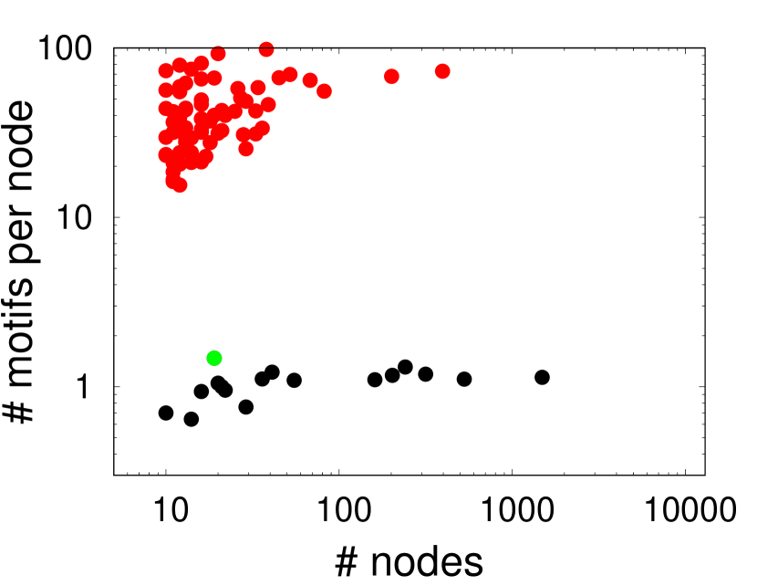
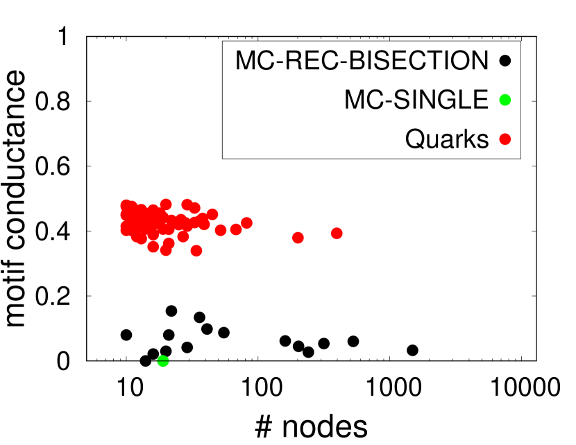
(a) reciprocal

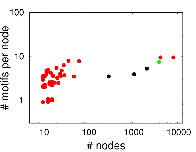
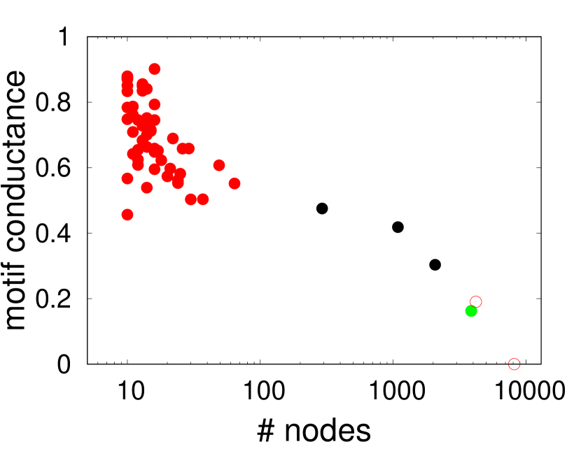
(b) out+

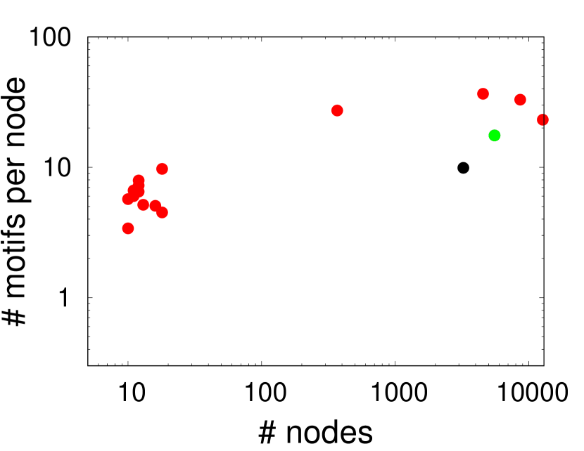
(c) acyclic

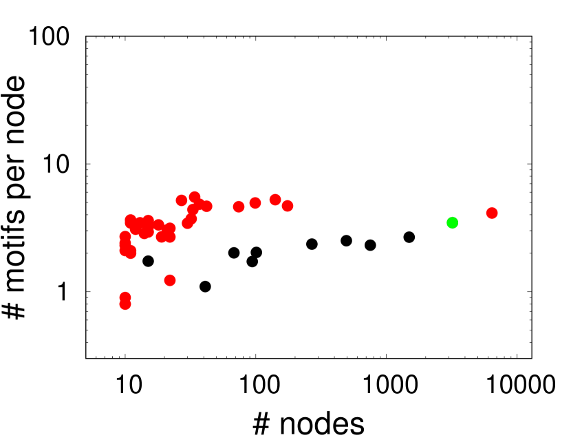
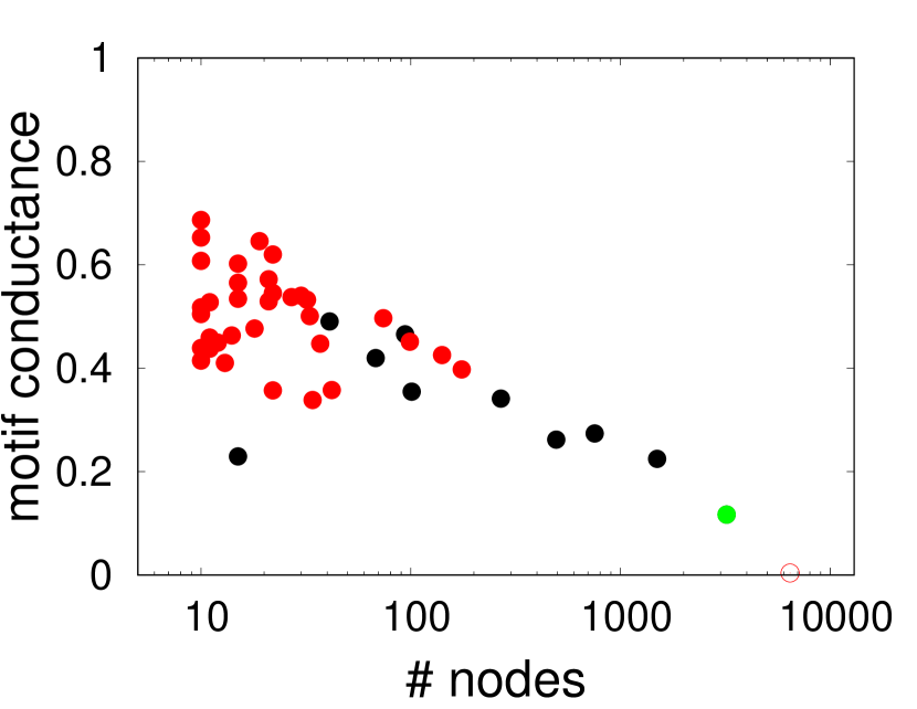
(d) cycle++

Figure 3. Comparison of the quark decomposition and MC (Benson et al., 2016) in EAT network. Top row shows the results for number of motifs per node, i.e., average motif degree, (higher is better) and the bottom row has the motif conductance (lower is better). We consider MC-Single, which obtains near-optimal motif conductance, and MC-Rec-Bisection, which is applied until the resulting cluster gets too small (less than 10 vertices) or high conductance (more than 0.5). For quark decomposition, we only show the $k$-quarks with at least 10 nodes. Each subgraph is denoted by a point; the size is shown on the $x$-axis and the metric is given on the $y$-axis. The large quarks for which the conductance computation requires the rest of the graph (since the size is more than the half) are denoted by red circles for completeness (conductances for those are not real).

Motifs. We instantiate the quark decomposition for directed networks by considering the edge and triangle motifs (Figure 1), corresponding to the $M$ and $N$ in Definition 2, respectively. Note that considering edge as motif $M$ is more advantageous than node. Since the edges are assigned quark numbers, $k$-quarks can overlap with each other. Also, role confusion does not happen for out+ and in+ as explained in Section 4.1.1. We also incorporate the reciprocity by considering the unidirectional and bidirectional edges separately, rather than treating each bidirectional edge as two unidirectional edges. This is because directed networks often have a significant percentage of bidirectional edges (also observed in Table 1) and those need to be treated differently, as discussed in  (Newman et al., 2002; Seshadhri et al., 2016). We use the vanilla edge as the motif $M$ and each of the seven directed triangles (Figure 1) as the motif $N$.

We first discuss the motif counts and quarks for directed triangles. Then we compare quarks with baselines using the EAT and foodweb networks. We finish by comparing the runtimes.

5.1.1. Motif counts and subgraphs

Table 1 lists the motif counts and maximum quark numbers for each motif. cycle is often the least common motif. Networks with significant fraction of bidirectional edges tend to contain reciprocal motifs the most. Note that the most frequent motif does not always yield the highest quark number. In particular, reciprocals are often concentrated in a small region, thus yield highly-dense subgraphs. For instance, en-wiki has 5.9M reciprocal and 163.3M acyclic motifs but the maximum quark numbers for those motifs are 29 and 26, respectively. This is because the maximum $k$-quark has 465 edges in the reciprocal case but has 9461 edges in acyclic. We also observe that the number of quarks are independent of the motif counts. For example, the most prevalent motif in EAT network is, by far, acyclic. However, acyclic yields only 447 $k$-quarks while the cycle+ locates 2826 subgraphs. Overall, the abundance of a particular motif does not imply the existence of dense subgraphs containing that motif.

5.1.2. Comparison with previous methods

We compare quark decomposition against the three baselines listed above. We use EAT network, a collection of word association norms where the nodes are English words and an edge $(u,v)$ implies that human subjects consider the word $v$ when they are shown the word $u$ as stimulus.

We first compare the quality of subgraphs given by the quark decomposition and MC algorithms (Benson et al., 2016) using motif conductance and average motif degree metrics. For quark decomposition, we only consider the $k$-quarks with at least 10 nodes. For MC algorithms, we consider MC-Single and MC-Rec-Bisection. Note that we aim to compare the ‘best’ clusters reported by the two algorithms and do not intend any comparison with respect to the number of clusters reported. Figure 3 gives the comparison for reciprocal, out+, acyclic, and cycle++ motifs (other motifs show similar results and omitted). For each subgraph, we report the size as well as the quality metric; number of motifs per node in the top row and the motif conductance in the bottom row. MC variants often give large subgraphs, always with very low conductance, as expected. MC-Single (optimal cluster) has more than 1000 nodes for out+, in+, acyclic, and cycle++. For cycle+, however, it has only five nodes. Quarks are often small, most in the range of 10-100 nodes, and have higher conductance scores. For out+ and cycle++, some quarks yield comparable conductance scores with MC-Rec-Bisection. We also observe that a quark for acylic has a better conductance than MC-Single (which is the near-optimal as shown in (Benson et al., 2016)). Regarding the average motif degrees (top row), quarks perform significantly better in all the motifs (note that y-axis is in log-scale). By definition of the quark (the connectivity constraint in particular), if the size is $n$, the number of motifs is at least $n-2$ (for $k=1$, a single motif is a valid subgraph and can be extended by a new node that creates a new motif, keeping the motif count $n-2$). This ensures a lower bound, $\frac{n-2}{n}$ (close to 1), for average motif degree in quarks. In general, quarks tend to be smaller in size when compared to MC results, have consistently higher average motif degrees, and comparable conductance scores for some motifs. Overall, the top-down partitioning approach in the motif clustering is likely to result in larger subgraphs in varying quality whereas the bottom-up computation in quark decomposition yields smaller subgraphs with larger average motif degrees.

Next we compare quark decomposition with TY (Takaguchi and Yoshida, 2016). For EAT network, TY reports maximum cycle-truss number of 3 and maximum flow-truss number of 10. For each maximum truss subgraph, we checked the quarks that are the most similar. Figure 4 presents the results for cycle-truss, flow-truss, and their corresponding quarks with size and average motif degree information. For cycle- and flow-truss, we calculate the induced cycle and acyclic motif degrees (i.e., bidirectional edges are not included). Next to each quark, we denote the size of its intersection with the truss. Various types of quarks are able to obtain almost all the nodes in those trusses. 70 of 77 nodes in cycle-truss are obtained with 15 quarks and all of the 45 nodes in flow-truss are given in 15 other quarks. This verifies the artificial over-representation of cycle- and flow-trusses due to the non-induced nature. Overall, treating the bidirectional edges as atomic units enables finding diverse subgraphs while correctly capturing the semantics of pairwise relationships.

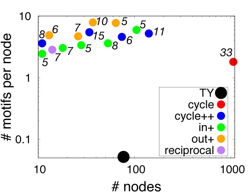
(a) cycle-truss vs. quarks

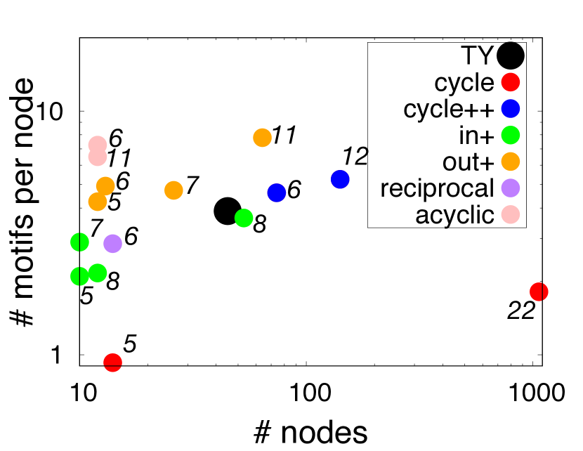
(b) flow-truss vs. quarks

Figure 4. Comparison of cycle- and flow-truss to quarks in EAT network. For each quark, size of its intersection with the truss is shown.

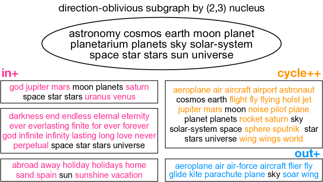
Figure 5. Comparison of a direction-oblivious $(2,3)$ nucleus and various quarks in EAT network. The common words in quarks and the nucleus is shown in black. Quarks by different motifs capture different contexts for those words. in+ provides multiple contexts for space, stars thanks to the fact that quarks are overlapping.

Lastly, we compare quarks with $(2,3)$ nucleus decomposition (Sarıyüce et al., 2015), which ignores edge directions. We observe that incorporating the edge directions results in more diverse subgraphs. The number of subgraphs (of any quality) obtained by each quark decomposition is significantly larger than what nucleus decomposition yields. As an anecdotal example, we show a subgraph found by the nucleus decomposition in Figure 5. The direction-oblivious subgraph contains words related to astronomy and space. Quark decompositions capture several diverse contexts related to those words. Thanks to the overlapping quarks, in+ finds two subgraphs that contain space and stars: one in astronomy theme (uranus, venus, …) and another in the religious context (god, eternity, …). It also finds another subgraph in the vacation theme (sun, holiday, sand, …). Out+ yields a subgraph in the air-flight context (sky, aircraft, wing, …). We also recognize that multiple meanings of the homonym words are reflected in various $k$-quarks. For instance, lie is reported in two subgraphs by cycle++: one is about incorrectness (falsehood, untruth, …) and the other is about staying at rest in the horizontal position (couch, rest, …). Overall, quark decompositions by various motifs can locate diverse contexts for a given word thanks to the motif-aware approach and overlapping nature of quarks.

5.1.3. Analysis of Florida Bay food web

Here we analyze the structure of Florida Bay food web network (foodweb) where the nodes are the compartments (i.e., organisms, species) and the edges are the directed carbon exchanges (i.e., $u\rightarrow v$ if $v$ eats $u$). Benson et al. showed that high-quality clusters (i.e., with low conductance) by MC only exist for out+, which implies that the organization of compartments is better described with out+ (as opposed to the common belief that acyclic is the key motif) (Benson et al., 2016). They also show that the 4 clusters by MC-k-means for out+ reflect the ground-truth subgroup classifications better than the state-of-the-art clustering algorithms such as spectral edge clustering (with k-means and recursive bisection) (Von Luxburg, 2007), InfoMap (Rosvall and Bergstrom, 2008), and Louvain method (Blondel et al., 2008).

We first compare the quarks for out+ with MC-k-means. We find 7 quarks for out+, so we consider MC-k-means with 7 clusters as well as with 4 clusters. The nodes that appear in multiple quarks are only considered to be part of their largest quark (other choices give similar results). Table 2 presents the results for two ground-truth classifications given in (Ulanowicz et al., 1998; Benson et al., 2016) by four metrics: Adjusted Rand Index (ARI), F1 score, Normalized Mutual Information (NMI), Purity (Manning et al., 2008). Quarks clearly outperforms MC-k-means variants in both classifications by all the metrics. One particular difference is that MC-k-means considers some macroinvertebrates like predatory crabs among the benthic predators of eels and toadfish whereas quark decomposition finds all macroinvertebrates in the same subgraph. We believe the main reason is that MC-k-means considers motif counts from the node-perspective while quark decomposition is based on the edges and their motif counts.

Table 2. foodweb classification results. Best in each row is in bold.

out+	Metric	Quarks	MC-k-means	MC-k-means
		(7 subgraphs)	w/ 4 clusters	w/ 7 clusters
Class 1	ARI	0.3627	0.3005	0.1485
	F1	0.4869	0.4574	0.3794
	NMI	0.5415	0.5040	0.4843
	Purity	0.5968	0.5645	0.5161
Class 2	ARI	0.3816	0.3265	0.1871
	F1	0.5675	0.5380	0.4601
	NMI	0.5206	0.4822	0.4309
	Purity	0.6452	0.6129	0.5645

Table 3. Runtimes for large directed networks (sec). Best result in each motif column is shown in bold.

	cycle		acyclic		out+		in+		cycle+		cycle++
	Q	M	Q	M	Q	M	Q	M	Q	M	Q	M
web-ND	0.34	3.31	4.26	16.8	0.62	6.3	2.11	8.54	0.53	10.01	0.78	9.86
amzn	0.74	3.54	3.29	79	2.25	132	1.92	105	1.18	5.29	3.23	107
wiki	28.9	14.0	112	18.2	10.9	16.4	21.1	17.7	20.5	20.2	47.8	16.8
soc-p	23.6	79	66.9	99	37.0	119	34.2	139	48.9	129	98.1	128
live-j	37.4	200	180	943	118	1135	126	1438	112	828	289	2248
en-w	900	501	7746	864	1511	799	1709	677	398	724	2223	677

We also consider acyclic and use role-aware quark decomposition (Algorithm 2) to determine the roles of the compartments in the resulting quarks. For an acyclic formed by $u$$\rightarrow$$v$, $u$$\rightarrow$$w$, and $v$$\rightarrow$$w$, we define $u$ as the prey orbit, $v$ as the balancer orbit, and $w$ as the predator orbit. The maximum quark obtained by QuarkDec (Algorithm 1) and RA-QuarkDec (Algorithm 2) is the same and contains 48 compartments. RA-QuarkDec assigns three quark numbers for each edge, corresponding to the three edge orbits in acyclic (each is a union of its nodes’ orbits). We determine the role profile for each node based on the quark numbers of its outgoing and incoming edges. The compartments that are dominantly predator are the birds including predatory ducks, big herons & egrets, greeb, and more. Dominantly prey compartments include clown goby, four types of zooplankton microfauna, and seven macroinvertebrates (including pink and herbivorous shrimps). Lastly, the ones that have the balancer role are the fishes, such as (bay) anchovy, sardines, and mojarra. Note that it is not possible to understand the roles of the compartments by QuarkDec since each edge has a single quark number. For instance, the average quark numbers of incoming and outgoing edges for predatory ducks and code goby are very close, which tells nothing about their roles.

5.1.4. Runtime performance.

We measure the runtime for quark decomposition and MC-Single on all directed networks, Table 3 lists the results for large networks. MC-Single (denoted M) gives only one near-optimal cluster and quark decomposition (denoted Q) finds all the quark numbers. Quark decomposition is faster than MC-Single for all motifs in web-ND, amazon, soc-pokec, and liveJournal. For some configurations, such as in+ in liveJournal, we observe up to 10x speedup. For en-wiki, however, MC-Single is faster for all motifs. Note that MC-Single runtime includes motif adjacency construction and spectral clustering to find one cluster. In order to find more clusters, spectral clustering needs to be run again. However, the spectral clustering takes 36% of the total time for en-wiki (on avg.), hence obtaining 10 clusters will increase the runtime by 4x. All in all, although MC-Single finds only one cluster, quark decomposition is faster for most networks and motifs, and a better choice especially when multiple subgraphs are targeted.

5.2. Signed-directed networks

Datasets. We use signed-directed networks that have categorical labels on edges to denote one-sided positive/negative relationships (no bidirectional edges). We have two Reddit hyperlink networks that have directed connections among the subreddits. reddit-body and reddit-title consider the positive and negative interactions among users who belong to different subreddits (Kumar et al., 2018). We considered the last interactions in the datasets. We also consider epinions, a who-trust-whom social network (Guha et al., 2004), and slashdot which contains the self-tagged friend/foe relationships (Kunegis et al., 2009). All are obtained from SNAP (Leskovec and Krevl, 2014). Table 4 gives the number of positive and negative edges, motif counts, and maximum quark numbers.

Motifs. We use edge and triangle motifs, corresponding to the $M$ and $N$ in Definition 2, respectively. This also ensures that quarks can overlap with each other. There is no bidirectional edge and there are twelve possible triangle motifs in total, as shown in Figure 6; four cycle motifs since there is a single orbit and eight acyclic motifs where each ++- and +-- appears in three different ways. We use the vanilla edge as $M$ and each of the twelve triangles (Figure 6) as $N$.

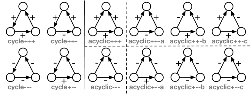
Figure 6. Signed directed triangle motifs.

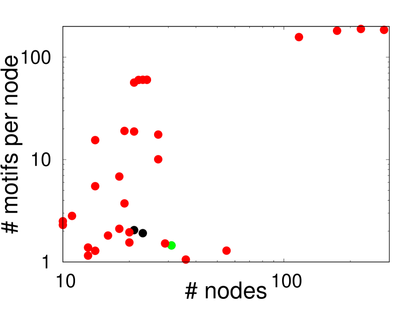
(a) Average motif degree

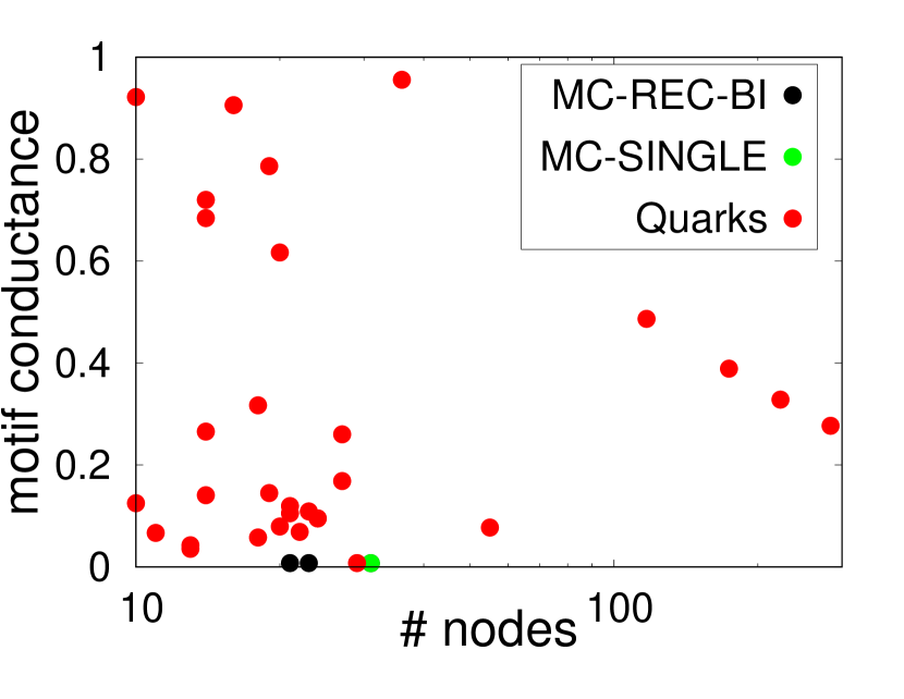
(b) Motif conductance

Figure 7. Comparison of quarks and MC (Benson et al., 2016) for acyclic+++ in reddit-body network with respect to the number of motifs per node (left, higher is better) and motif conductance (right, lower is better). Subgraphs with at least 10 nodes are shown. Each subgraph is denoted by a point; size is on the x-axis and metric is on the y-axis.

5.2.1. Motif counts and quark numbers

Acyclic variants are significantly more common than the cycles in all networks. Among the cycle variants, +++ is the most prevalent in reddit networks and --- is the least common in all. This is also coherent with the structural balance theory (Easley and Kleinberg, 2010), which states that the triangles with an odd number of negative links are rare. However, cycle++- is more common than the other cycles in the epinions network. This might be due to hierarchical status among the nodes; the lower status nodes are likely to trust the ones with higher status but the reverse is not true. The ratio of balanced triangles is 0.8 for reddit networks but 0.42 for epinions. Per the maximum quark numbers, we observe a correlation with the motif counts. Among all, only acyclic+++ yields non-trivial subgraphs with large quark numbers. Cycle variants fail to give significant quarks.

Table 4. Signed datasets. $|V|$, $|E|$, $|E_{+}|$, and $|E_{-}|$ are the number of nodes, edges, positive, and negative edges. Motif counts (see Figure 6) and corresponding maximum quark numbers are also shown.

			red-body	red-title	epinions	slashdot
$|V|$			34.7K	52.9K	125.8K	74.3K
$|E|$			110.8K	205.5K	581.6K	420.5K
$|E_{+}|$			102.5K	188.7K	465.4K	311.3K
$|E_{-}|$			8.3K	16.8K	116.3K	109.2K
		$+++$	4.9K	7.8K	14.1K	1.2K
		$++-$	1.3K	1.9K	34.2K	1.3K
	cycle	$+--$	166	233	10.9K	702
		$---$	9	13	745	86
		$+++$	145.7K	592.9K	1.1M	125.0K
motif		$++-a$	20.0K	88.8K	37.1K	15.3K
counts		$++-b$	22.1K	88.8K	14.1K	9.0K
	acylic	$++-c$	18.0K	59.3K	115.0K	15.7K
		$+--a$	3.4K	10.8K	88.5K	11.8K
		$+--b$	3.1K	10.8K	8.3K	7.8K
		$+--c$	6.2K	26.6K	92.1K	30.4K
		$---$	1.1K	3.5K	39.7K	9.0K
max.	cycle	all	1	1-2	1-2	1
quark	acyclic	$+++$	15	20	15	6
numbers		others	2-3	2-4	2-5	2-5

5.2.2. Comparison with MC

We compare the $k$-quarks with the MC-Single and MC-Rec-Bisection for acyclic+++ motif in Figure 7. Some quarks are able to obtain very low conductance scores, close to MC results. For the average motif degrees, quarks significantly outperform MC-Rec-Bisection. In particular, one quark has 284 nodes with average motif degree of 185.2.

One of the quarks by acyclic+++ has 21 subreddits about rappers/singers, such as kanye and kendricklamar. The ones which praised the others but have not received much praise (the white node in acyclic in Figure 1) are boogalized, runthejewels, and  charlieputh. The last two are a young rapper duo and a new Canadian singer, respectively, with 6.6K and 279 members. On the other hand, the subreddits that got praised by the others but have not reciprocated (the black node in acyclic) are theweeknd, frankocean, and kidcudi. Those are experienced ones (active since 2010, 2005, and 2003) with tens of thousands of members in their subreddits.

5.3. Node-labeled networks

Datasets. Here we consider node-labeled undirected networks. We use the Facebok100 dataset that contains the complete Facebook networks of 100 American colleges from a single-day snapshot in September 2005 (Traud et al., 2012). Each node has multiple labels, here we only consider the genders of the nodes (there are only two available in the dataset; female and male) and use quark decomposition to find subgraphs that have balanced gender ratios, i.e., close number of females and males. Excluding the female-only institutions, the overall average female ratio is $\%48.5$ and there are 57 networks with less than $50\%$ female. We choose 18 networks with the lowest female ratio (all have $<45\%$), Table 5 gives a partial list.

Table 5. Node-labeled graphs. Statistics and avg. of the female ratios in nuclei and quarks are given. $V_{f}$ denotes the set of female nodes. (2,3)n and (3,4)n are the nucleus decompositions.

	$|V|$	$|E|$	$\frac{|V_{f}|}{|V|}$	edge, triangle			triangle, 4-clique
				(2,3)n	Quarks		(3,4)n	Quarks
					FMM	FFM		FMMM	FFMM	FFFM
Mich67	3.7K	81.9K	25%	23.0%	45.0%	50.0%	24.5%	40.0%	45.0%	51.6%
Caltech36	769	16.7K	30%	39.4%	46.0%	52.0%	38.5%	43.1%	50.2%	52.8%
Carnegie49	6.6K	250.0K	37%	32.6%	49.0%	52.5%	38.5%	43.5%	49.5%	54.9%
MIT8	6.4K	251.3K	37%	38.8%	48.0%	52.1%	42.0%	44.3%	50.3%	53.9%
Stanford3	11.6K	568.3K	40%	46.8%	48.1%	49.0%	44.1%	45.4%	49.2%	55.4%
Cornell5	18.7K	790.8K	44%	44.3%	47.6%	51.8%	45.6%	43.7%	48.7%	54.9%
Penn94	41.6K	1.4M	44%	49.7%	48.4%	51.4%	52.1%	44.0%	49.8%	55.8%
UPenn7	14.9K	686.5K	44%	37.3%	48.8%	51.1%	46.4%	45.1%	50.4%	55.4%
Average of 18 networks:			40%	42.5%	48.2%	51.5%	44.1%	44.4%	49.7%	54.7%

Motifs. We instantiate the quark decomposition in five ways, where F/M denotes the female/male nodes: (1) $M$ is vanilla edge and $N$ is triangle in the following two forms: FMM and FFM; and (2) $M$ is vanilla triangle, $N$ is four-clique in the following three forms: FMMM, FFMM, and FFFM. Also, there is no role confusion for any variant since the graph is undirected and node labels ensure that an edge cannot serve in different roles in its triangles in (1) (likewise for (2)).

5.3.1. Finding gender balanced subgraphs

Algorithmic fairness is one of the most important problems in today’s automated world (Kearns and Roth, 2019). Algorithms can amplify the implicit bias in the data, particularly based on the protected attributes like gender, race, ethnicity, and this can lead to unwanted consequences in criminal justice system, hiring, credit scoring, and more (Barocas et al., 2017). The bias in the network data is more complicated; regarding the gender attribute, for example, the problem is not only the imbalanced gender distribution but also how each gender category is connected to the other categories. There are a few studies that analyze the implications on information diffusion (Stoica and Chaintreau, 2019; Jalali et al., 2020). In this context, the community structure in the network plays an important role and algorithms that do not actively consider the protected attributes are likely to fail getting fair results. Algorithms that can find balanced communities even when there is an imbalance in the input network are essential. Here we use quark decomposition to find subgraphs with balanced gender ratios. As explained above, we set the input motif $N$ in ways to reflect the characteristics of gender balanced subgraphs.

Table 5 gives the female ratios in quarks in comparison to the label-oblivious nucleus decomposition algorithms (Sarıyüce et al., 2015). For each network, we find the leaf quarks (Definition 3) and nuclei with at least 10 nodes, calculate the female ratio in each quark or nucleus, and then take the average of those ratios. We also show the average ratios across all the 18 datasets at the bottom. The average female ratio of all the networks is $40.3\%$. $(2,3)$-nuclei have a bit better number, $42.5\%$. Quarks for FMM get $48.2\%$ and the ratios are consistently good for all the networks, varying between $45\%-51.3\%$. This significant jump from $(2,3)$-nuclei is due to the fact that each edge has to participate in a number of FMM triangles. Quarks for FFM give an even better ratio, $51.5\%$. $(3,4)$-nuclei are larger in number and also denser than $(2,3)$. Its average female ratio ($44.1\%$) is also a bit better than $(2,3)$-nuclei. Quarks for FMMM are very close to $(3,4)$-nuclei but more consistent. FFMM achieves $49.7\%$ and FFFM gets the best: $54.7\%$. Note that results get better for the motifs with larger female ratio: FMMM ¡ FMM ¡ FFMM ¡ FFM ¡ FFFM.

Quarks cannot provide a good theoretical lower bound for the female ratio since there is no size constraint in the quark definition. For instance, a 1-quark for FFM can possibly be formed by a pair of connected female nodes and $n$ male nodes that are connected to both females; the female ratio would be $2/(n+2)$ in this case. But in practice, quarks with female-dominant motifs yield dense subgraphs with high female ratios. Even with FMM, which implies a 1/3 ratio (smaller than the average female ratio of the datasets), quarks can obtain better results than the label-oblivious (2,3)-nuclei.

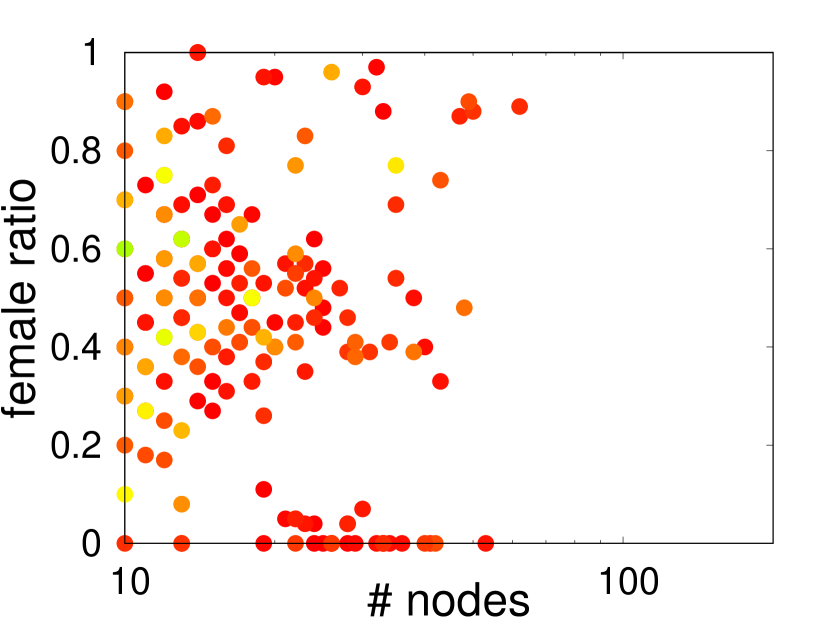
(a) $(3,4)$ nuclei

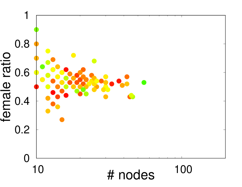
(b) Quarks by FFFM

Figure 8. Comparison of the female ratios in subgraphs obtained by quark (FFFM) and $(3,4)$-nucleus decompositions for UPenn7. For each subgraph, size is given on the x-axis, female ratio is shown on the y-axis, and the edge density is color-coded.

We also show all the subgraphs with size, edge density, and female ratio information obtained by quark and nucleus decompositions in UPenn7 network.  Figure 8 gives $(3,4)$-nuclei and quarks for FFFM on UPenn7 network. Quarks are consistently gender balanced when compared to the nuclei; no quark with less than $25\%$ female ratio exists. Note that there is a bit degradation in the number and density of the quarks for FFFM: 216 subgraphs with 0.88 avg. edge density, compared to the 230 $(3,4)$ nuclei with avg. density 0.94. Given the consistently high female ratios, we believe that this is an affordable loss in quality.

6. Discussion

Quark decomposition offers a principled approach for motif-driven dense subgraph discovery in heterogeneous networks by successfully regularizing the motif degrees to quark numbers. Our evaluation shows that the $k$-quarks can find dense subgraphs according to a given motif. Role-aware variant solves the role confusion problem by creating multiple quark numbers for each motif $M$. Overall, quark decomposition is versatile, efficient, and extendible.

For future work, it would be interesting to investigate the other byproducts of the quark decomposition, such as hierarchy structure. Our initial results show limited success; detailed and meaningful hierarchies are rare for the most motifs. Theoretical and empirical analysis of the impact of the input motifs, $M,N$, on the hierarchy structure would be interesting . Also, adapting the quark decomposition for numerical attributes on nodes/edges would be promising.

- (1)
- CCR (2021) 2021. Center for Computational Research, University at Buffalo. http://hdl.handle.net/10477/79221.
- Ahmed et al. (2016) N. K. Ahmed, J. Neville, R. A. Rossi, N. Duffield, and T. L. Willke. 2016. Graphlet Decomposition: Framework, Algorithms, and Applications. KAIS (2016), 1–32.
- Aksoy et al. (2017) S. Aksoy, T. G. Kolda, and A. Pinar. 2017. Measuring and Modeling Bipartite Graphs with Community Structure. Journal of Complex Networks 5, 4 (2017), 581–603.
- Almeida et al. (2011) Hélio Almeida, Dorgival Guedes, Wagner Meira, and Mohammed J Zaki. 2011. Is there a best quality metric for graph clusters?. In Joint European conference on machine learning and knowledge discovery in databases. Springer, 44–59.
- Alvarez-Hamelin et al. (2006) J. Ignacio Alvarez-Hamelin, Alain Barrat, and Alessandro Vespignani. 2006. Large scale networks fingerprinting and visualization using the k-core decomposition. In NIPS. 41–50.
- Barocas et al. (2017) Solon Barocas, Moritz Hardt, and Arvind Narayanan. 2017. Fairness in machine learning. NIPS Tutorial 1 (2017).
- Batagelj and Zaversnik (2003) V. Batagelj and M. Zaversnik. 2003. An O(m) Algorithm for Cores Decomposition of Networks. Technical Report cs/0310049. Arxiv.
- Benson et al. (2016) Austin R. Benson, David F. Gleich, and Jure Leskovec. 2016. Higher-order organization of complex networks. Science 353, 6295 (2016), 163–166.
- Blondel et al. (2008) Vincent D Blondel, Jean-Loup Guillaume, Renaud Lambiotte, and Etienne Lefebvre. 2008. Fast unfolding of communities in large networks. Journal of statistical mechanics: theory and experiment 2008, 10 (2008), P10008.
- Carmi et al. (2007) Shai Carmi, Shlomo Havlin, Scott Kirkpatrick, Yuval Shavitt, and Eran Shir. 2007. A model of Internet topology using k-shell decomposition. PNAS 104, 27 (2007), 11150–11154.
- Carranza et al. (2020) Aldo G Carranza, Ryan A Rossi, Anup Rao, and Eunyee Koh. 2020. Higher-order Clustering in Complex Heterogeneous Networks. In Proceedings of the 26th ACM SIGKDD International Conference on Knowledge Discovery & Data Mining. 25–35.
- Cohen (2008) J. Cohen. 2008. Trusses: Cohesive subgraphs for social network analysis. National Security Agency Technical Report (2008).
- Du et al. (2009) X. Du, R. Jin, L. Ding, V. E. Lee, and J. H. Thornton Jr. 2009. Migration motif: a spatial - temporal pattern mining approach for financial markets.. In KDD. 1135–1144.
- Easley and Kleinberg (2010) David Easley and Jon Kleinberg. 2010. Networks, crowds, and markets. (2010).
- Fang et al. (2020) Yixiang Fang, Xin Huang, Lu Qin, Ying Zhang, Wenjie Zhang, Reynold Cheng, and Xuemin Lin. 2020. A survey of community search over big graphs. The VLDB Journal 29, 1 (2020), 353–392.
- Fang et al. (2019) Yixiang Fang, Kaiqiang Yu, Reynold Cheng, Laks VS Lakshmanan, and Xuemin Lin. 2019. Efficient algorithms for densest subgraph discovery. PVLDB 12, 11 (2019), 1719–1732.
- Fratkin et al. (2006) E. Fratkin, B. T. Naughton, D. L. Brutlag, and S. Batzoglou. 2006. MotifCut: regulatory motifs finding with maximum density subgraphs.. In ISMB (2006-08-28). 156–157.
- Gionis et al. (2013) A. Gionis, F. Junqueira, V. Leroy, M. Serafini, and I. Weber. 2013. Piggybacking on Social Networks. PVLDB 6, 6 (2013), 409–420.
- Gleich and Seshadhri (2012) David F. Gleich and C. Seshadhri. 2012. Vertex Neighborhoods, Low Conductance Cuts, and Good Seeds for Local Community Methods. In KDD. 597–605.
- Goldberg (1984) A. V. Goldberg. 1984. Finding a Maximum Density Subgraph. Technical Report. Berkeley, CA, USA.
- Guha et al. (2004) Ramanthan Guha, Ravi Kumar, Prabhakar Raghavan, and Andrew Tomkins. 2004. Propagation of trust and distrust. In WWW. 403–412.
- Hu et al. (2019) Jiafeng Hu, Reynold Cheng, Kevin Chen-Chuan Chang, Aravind Sankar, Yixiang Fang, and Brian YH Lam. 2019. Discovering maximal motif cliques in large heterogeneous information networks. In 2019 IEEE (ICDE). IEEE, 746–757.
- Huang et al. (2014) Xin Huang, Hong Cheng, Lu Qin, Wentao Tian, and Jeffrey Xu Yu. 2014. Querying K-truss Community in Large and Dynamic Graphs. In SIGMOD. 1311–1322.
- Jain and Seshadhri (2017) Shweta Jain and C. Seshadhri. 2017. A Fast and Provable Method for Estimating Clique Counts Using Turán’s Theorem. In WWW. 441–449.
- Jalali et al. (2020) Zeinab S. Jalali, Weixiang Wang, Myunghwan Kim, Hema Raghavan, and Sucheta Soundarajan. 2020. On the Information Unfairness of Social Networks. 613–521.
- Jin et al. (2009) R. Jin, Y. Xiang, N. Ruan, and D. Fuhry. 2009. 3-HOP: a high-compression indexing scheme for reachability query. In SIGMOD Conf. 813–826.
- Kearns and Roth (2019) Michael Kearns and Aaron Roth. 2019. The ethical algorithm: The science of socially aware algorithm design. Oxford University Press.
- Kiss et al. (1973) George R Kiss, Christine Armstrong, Robert Milroy, and James Piper. 1973. An associative thesaurus of English and its computer analysis. The computer and literary studies (1973), 153–165.
- Kitsak et al. (2010) Maksim Kitsak, Lazaros K Gallos, Shlomo Havlin, Fredrik Liljeros, Lev Muchnik, H Eugene Stanley, and Hernán A Makse. 2010. Identification of influential spreaders in complex networks. Nature physics 6, 11 (2010), 888.
- Kumar et al. (1999) R. Kumar, P. Raghavan, S. Rajagopalan, and A. Tomkins. 1999. Trawling the Web for Emerging Cyber-communities. In WWW. 1481–1493.
- Kumar et al. (2018) Srijan Kumar, William L Hamilton, Jure Leskovec, and Dan Jurafsky. 2018. Community interaction and conflict on the web. In WWW. 933–943.
- Kunegis et al. (2009) Jérôme Kunegis, Andreas Lommatzsch, and Christian Bauckhage. 2009. The slashdot zoo: mining a social network with negative edges. In WWW. ACM, 741–750.
- Lee et al. (2010) V. E. Lee, N. Ruan, R. Jin, and C. Aggarwal. 2010. A Survey of Algorithms for Dense Subgraph Discovery. In Managing and Mining Graph Data. Vol. 40.
- Leskovec and Krevl (2014) Jure Leskovec and Andrej Krevl. 2014. SNAP Datasets.
- Leskovec et al. (2008) Jure Leskovec, Kevin J. Lang, Anirban Dasgupta, and Michael W. Mahoney. 2008. Statistical Properties of Community Structure in Large Social and Information Networks (WWW ’08). ACM, 695–704.
- Li et al. (2019) Pei Li, Ling Huang, Chang-Dong Wang, and Jian-Huang Lai. 2019. EdMot: An Edge Enhancement Approach for Motif-aware Community Detection. In SIGKDD. 479–487.
- Malliaros et al. (2016) Fragkiskos D Malliaros, Maria-Evgenia G Rossi, and Michalis Vazirgiannis. 2016. Locating influential nodes in complex networks. Scientific reports 6 (2016), 19307.
- Manning et al. (2008) Christopher D Manning, Hinrich Schütze, and Prabhakar Raghavan. 2008. Introduction to information retrieval. Cambridge university press.
- Melckenbeeck et al. (2018) Ine Melckenbeeck, Pieter Audenaert, Didier Colle, and Mario Pickavet. 2018. Efficiently counting all orbits of graphlets of any order in a graph using autogenerated equations. Bioinformatics 34, 8 (2018), 1372–1380.
- Milo et al. (2002) Ron Milo, Shai Shen-Orr, Shalev Itzkovitz, Nadav Kashtan, Dmitri Chklovskii, and Uri Alon. 2002. Network motifs: simple building blocks of complex networks. Science 298, 5594 (2002), 824–827.
- Newman et al. (2002) Mark EJ Newman, Stephanie Forrest, and Justin Balthrop. 2002. Email networks and the spread of computer viruses. Physical Review E 66, 3 (2002), 035101.
- Peng et al. (2014) Chengbin Peng, Tamara G Kolda, and Ali Pinar. 2014. Accelerating community detection by using k-core subgraphs. arXiv preprint arXiv:1403.2226 (2014).
- Pinar et al. (2017) Ali Pinar, C. Seshadhri, and Vaidyanathan Vishal. 2017. ESCAPE: Efficiently Counting All 5-Vertex Subgraphs (WWW ’17). 1431–1440.
- Pržulj (2007) Nataša Pržulj. 2007. Biological network comparison using graphlet degree distribution. Bioinformatics 23, 2 (2007), e177–e183.
- Rosvall and Bergstrom (2008) Martin Rosvall and Carl T Bergstrom. 2008. Maps of random walks on complex networks reveal community structure. PNAS 105, 4 (2008), 1118–1123.
- Saito and Yamada (2006) K. Saito and T. Yamada. 2006. Extracting Communities from Complex Networks by the k-dense Method. In ICDMW.
- Sarajlić et al. (2016) Anida Sarajlić, Noël Malod-Dognin, Ömer Nebil Yaveroğlu, and Nataša Pržulj. 2016. Graphlet-based characterization of directed networks. Scientific reports 6 (2016), 35098.
- Sariyüce and Pinar (2016) A. Erdem Sariyüce and Ali Pinar. 2016. Fast Hierarchy Construction for Dense Subgraphs. Proc. VLDB Endow. 10, 3 (Nov. 2016), 97–108.
- Sariyüce and Pinar (2018) A. Erdem Sariyüce and Ali Pinar. 2018. Peeling Bipartite Networks for Dense Subgraph Discovery. In WSDM.
- Sarıyüce et al. (2015) A. Erdem Sarıyüce, C. Seshadhri, A. Pınar, and Ü. V. Çatalyürek. 2015. Finding the Hierarchy of Dense Subgraphs Using Nucleus Decompositions. In WWW (Florence, Italy). 927–937.
- Sariyüce et al. (2017) A. Erdem Sariyüce, C. Seshadhri, Ali Pinar, and Ümit V. Çatalyürek. 2017. Nucleus Decompositions for Identifying Hierarchy of Dense Subgraphs. ACM Trans. Web 11, 3, Article 16 (July 2017), 27 pages. https://doi.org/10.1145/3057742
- Seidman (1983) S. B. Seidman. 1983. Network structure and minimum degree. Social Networks 5, 3 (1983), 269–287.
- Seshadhri et al. (2016) C Seshadhri, Ali Pinar, Nurcan Durak, and Tamara G Kolda. 2016. Directed closure measures for networks with reciprocity. Journal of Complex Networks 5, 1 (2016), 32–47.
- Seshadhri et al. (2014) C. Seshadhri, Ali Pinar, and Tamara G. Kolda. 2014. Triadic Measures on Graphs: The Power of Wedge Sampling. Statistical Analysis and Data Mining 7, 4 (2014), 294–307.
- Stoica and Chaintreau (2019) Ana-Andreea Stoica and Augustin Chaintreau. 2019. Fairness in Social Influence Maximization. In Companion Proceedings of The 2019 Web Conference. 569–574.
- Sun and Han (2012) Yizhou Sun and Jiawei Han. 2012. Mining heterogeneous information networks: principles and methodologies. Synthesis Lectures on Data Mining and Knowledge Discovery 3, 2 (2012), 1–159.
- Sun et al. (2011) Yizhou Sun, Jiawei Han, Xifeng Yan, Philip S Yu, and Tianyi Wu. 2011. Pathsim: Meta path-based top-k similarity search in heterogeneous information networks. Proceedings of the VLDB Endowment 4, 11 (2011), 992–1003.
- Takaguchi and Yoshida (2016) Taro Takaguchi and Yuichi Yoshida. 2016. Cycle and flow trusses in directed networks. Royal Society open science 3, 11 (2016), 160270.
- Traud et al. (2012) Amanda L Traud, Peter J Mucha, and Mason A Porter. 2012. Social structure of facebook networks. Physica A: Statistical Mechanics and its Applications 391, 16 (2012), 4165–4180.
- Tsourakakis (2015) C. Tsourakakis. 2015. The K-clique Densest Subgraph Problem (WWW ’15). 1122–1132.
- Tsourakakis et al. (2017) C. E. Tsourakakis, J. Pachocki, and M. Mitzenmacher. 2017. Scalable Motif-aware Graph Clustering (WWW ’17). 1451–1460.
- Ulanowicz et al. (1998) Robert E Ulanowicz, Cristina Bondavalli, and MS Egnotovich. 1998. Network analysis of trophic dynamics in south florida ecosystem, fy 97: The florida bay ecosystem. Annual Report to the United States Geological Service Biological Resources Division Ref. No.[UMCES] CBL (1998), 98–123.
- Von Luxburg (2007) Ulrike Von Luxburg. 2007. A tutorial on spectral clustering. Statistics and computing 17, 4 (2007), 395–416.
- Wang et al. (2016) Hongzhi Wang, Jianzhong Li, and Hong Gao. 2016. Efficient entity resolution based on subgraph cohesion. Knowledge and information systems 46, 2 (2016), 285–314.
- Xie et al. (2013) Jierui Xie, Stephen Kelley, and Boleslaw K. Szymanski. 2013. Overlapping Community Detection in Networks: The State-of-the-art and Comparative Study. ACM Comput. Surv. 45, 4, Article 43 (Aug. 2013), 35 pages.
- Yaveroğlu et al. (2014) Ömer Nebil Yaveroğlu, Noël Malod-Dognin, Darren Davis, Zoran Levnajic, Vuk Janjic, Rasa Karapandza, Aleksandar Stojmirovic, and Nataša Pržulj. 2014. Revealing the hidden language of complex networks. Scientific reports 4 (2014), 4547.