From viral evolution to spatial contagion: a biologically modulated Hawkes model

Abstract

Mutations sometimes increase contagiousness for evolving pathogens. During an epidemic, scientists use viral genome data to infer a shared evolutionary history and connect this history to geographic spread. We propose a model that directly relates a pathogen’s evolution to its spatial contagion dynamics—effectively combining the two epidemiological paradigms of phylogenetic inference and self-exciting process modeling—and apply this phylogenetic Hawkes process to a Bayesian analysis of 23,422 viral cases from the 2014-2016 Ebola outbreak in West Africa. The proposed model is able to detect individual viruses with significantly elevated rates of spatiotemporal propagation for a subset of 1,610 samples that provide genome data. Finally, to facilitate model application in big data settings, we develop massively parallel implementations for the gradient and Hessian of the log-likelihood and apply our high performance computing framework within an adaptively preconditioned Hamiltonian Monte Carlo routine.

Keywords

Bayesian phylogeography; Ebola virus; parallel computing; spatiotemporal Hawkes processes.

1 Introduction

The COVID-19 pandemic has demonstrated the need for new scientific tools for the analysis and prediction of viral contagion across human landscapes. The mathematical characterization of the complex relationships underlying pathogen genetics and spatial contagion stands as a central challenge of 21st century epidemiology. We approach this task by unifying two distinct probabilistic approaches to viral modeling. On the one hand, Bayesian phylogenetics (Sinsheimer et al., 1996; Yang and Rannala, 1997; Mau et al., 1999; Suchard et al., 2001) uses genetic sequences from a limited collection of viral samples to integrate over high-probability shared evolutionary histories in the form of phylogenies or family trees. On the other hand, self-exciting, spatiotemporal Hawkes processes (Reinhart, 2018) model spatial contagion by allowing an observed event to increase the probability of additional observations nearby and in the immediate future.

Both modeling paradigms come with their own advantages. For Bayesian phylogenetics, the past twenty years have witnessed a slew of high-impact scientific studies in viral epidemiology (Rambaut et al., 2008; Smith et al., 2009; Faria et al., 2014; Gire et al., 2014; Dudas et al., 2017; Boni et al., 2020) and the rise of powerful computing tools facilitating inference from expressive, hierarchical models of phylogenies and evolving traits (Ronquist et al., 2012; Suchard et al., 2018). Unfortunately, the number of evolutionary trees to integrate over explodes with the number of viral samples analyzed (Felsenstein, 1978), so Bayesian phylogenetic analyses typically restrict to a relatively small number of viral samples, at most totaling a few thousand. The fact that viral cases that undergo genetic sequencing usually represent a small subset of the total case count exacerbates this issue. Thus, failure to detect phylogenetic clades that represent novel strains on account of computational and surveillance limitations always remains a possibility. Until now, these weaknesses have also held for the sub-discipline of Bayesian phylogeography, which attempts to relate viral evolutionary histories to geographic spread as represented by (typically Brownian) phylogenetic diffusions. These models describe viral spread through either discretized (Lemey et al., 2009) or continuous (Lemey et al., 2010) space, but both approaches induce their own form of bias (Holbrook et al., 2020). In the face of these shortcomings, Bayesian phylogeography needs new tools for directly modeling spatial contagion.

	Traditional Bayesian phylogenetics	Hawkes processes
Observational limit	$N$ in low thousands	$N$ in high tens-of-thousands
Biological insight	Evolutionary history	None
Genetic sequencing	Required	Not required
Spatiotemporal data	Not required	Required
Geographic spread	Not modeled	Modeled
Large-scale transport	Does not induce bias	Induces bias

Table 1: Comparison of two probabilistic modeling paradigms within viral epidemiology, the combination of which represents a new tool for Bayesian phylogeography.

Hawkes processes (Hawkes, 1971a, b, 1972, 1973, 2018) are widely applicable point process models for generally viral or contagious phenomena, such as earthquakes and aftershocks (Hawkes, 1973; Ogata, 1988; Zhuang et al., 2004; Fox et al., 2016), financial stock trading (Bacry et al., 2015; Hawkes, 2018), viral content on social media (Rizoiu et al., 2017; Kobayashi and Lambiotte, 2016), gang violence (Mohler et al., 2013; Mohler, 2014; Loeffler and Flaxman, 2018; Park et al., 2019; Holbrook et al., 2021) and wildfires (Schoenberg, 2004). Unsurprisingly, Hawkes processes are natural models for the contagion dynamics of biological viruses as well. Kim (2011) uses spatiotemporal Hawkes processes (Reinhart, 2018), which model viral cases as unmarked events in space and time, to model the spread of avian influenza virus (H5N1). Meyer et al. (2014) incorporate power laws to describe spatial contagion dynamics and model meningococcal disease in Germany from 2001 to 2008. While Rizoiu et al. (2018) do not model epidemiological data, they do draw connections between epidemiological SIR models and Hawkes processes, showing that the rate of events in the SIR model is equal to that of a finite-population Hawkes model. Kelly et al. (2019) apply a temporal nonparametric Hawkes process to the 2018-2019 Ebola outbreak in the Democratic Republic of the Congo and successfully generate accurate disease prevalence forecasts. Chiang et al. (2020) model COVID-19 cases and deaths in the U.S. at the county level using spatially indexed mobility and population data to modify the process conditional intensity. Most recently, Bertozzi et al. (2020) compare the performance of a temporal Hawkes process model with temporally evolving conditional intensity to that of SIR and SEIR models for modeling regional COVID-19 case dynamics.

Because such Hawkes processes do not involve genetic information, one may apply the model to a much larger collection of cases, i.e., those for which a timestamp and spatial coordinates are available. Moreover, recent successes in scaling Hawkes process inference to a big data setting enable inference from observations numbered in the high tens-of-thousands (Holbrook et al., 2021; Yuan et al., 2021). This ability to interface with an order of magnitude more cases represents a major benefit of the Hawkes process in comparison to the Bayesian phylogenetic paradigm, but the trade-off is that conclusions drawn from a Hawkes process analysis are devoid of explicit biological insight. It is possible for the model to attribute self-exciting dynamics to nearby viral cases that are only distantly related on the phylogenetic tree. Finally, these processes do not immediately account for viral spread through large-scale transportation networks (Brockmann and Helbing, 2013; Holbrook et al., 2020) but attribute events resulting from such contagion to a ‘background’ process.

In the following, we construct a Bayesian hierarchical model that allows both modeling approaches to support each other. This model (Figure 1) learns phylogenetic trees that describe the evolutionary history of the subset of observations that yield genetic sequencing and uses this history to inform the distribution of a latent relative rate or productivity (Schoenberg et al., 2019; Schoenberg, 2020) for each virus in this limited set. In turn, these virus-specific rates modify the rate of self-excitation of a spatiotemporal Hawkes process describing the contagion of all viruses, sequenced or not. We use a Metropolis-within-Gibbs strategy to jointly infer all parameters and latent variables of our phylogenetic Hawkes process and overcome the $O(N^{2})$ computational complexity of the Hawkes process likelihood by incorporating the modified likelihood in the hpHawkes open-source, high-performance computing library (Holbrook et al., 2021) available at https://github.com/suchard-group/hawkes. Within the same library, we also develop multiple parallel computing algorithms for the log-likelihood gradient and Hessian with respect to the model’s virus-specific rates. GPU-based implementations of these gradient and Hessian calculations score hundred-fold speedups over single-core computing and help overcome quadratic complexity in the context of an adaptively preconditioned Hamiltonian Monte Carlo (Neal, 2011). These speedups prove useful in our analysis of 23,422 viral cases from the 2014-2016 Ebola outbreak in West Africa.

2 Methods

We develop the phylogenetic Hawkes process and its efficient inference in the following sections. Importantly, our proposed hierarchical model integrates both sequenced and unsequenced viral case data, representing a significant and clear contribution insofar as:

1. the percentage of confirmed viral cases sequenced during an epidemic is often in the single digits (Wadman, 2021);

2. and previous phylogeographic models have failed to leverage additional information provided by geolocated, unsequenced case data.

We address this shortcoming by constructing a new hierarchical model that both models all spatiotemporal data with a Hawkes process (Section 2.1) and allows an inferred evolutionary history in the form of a phylogenetic tree to influence dependencies between relative rates of contagion (Section 2.2) for the small subset of viral cases for which genome data are available. We believe that this approach is altogether novel.

2.1 Spatiotemporal Hawkes process for viral contagion

Hawkes processes (Hawkes, 1971a, b, 1972, 2018) constitute a useful class of inhomgeneous Poisson point processes (Daley and Jones, 2003) for which individual events contribute to an increased rate of future events. Spatiotemporal Hawkes processes (Reinhart, 2018) are marked Hawkes processes with spatial coordinates for marks (Daley and Jones, 2003). We are interested in spatiotemporal Hawkes processes with infinitesimal rate

$$\lambda(\mathbf{x},t)=\mu(\mathbf{x})+\xi(\mathbf{x},t)=\mu(\mathbf{x})+\sum_{t_{n}<t}g_{n}(\mathbf{x}-\mathbf{x}_{n},t-t_{n})\,,$$

where $\mathbf{x}\in\mathbb{R}^{D}$, $t\in\mathbb{R}^{+}$ and the subscript $n$ indicates that the usual triggering function $g(\cdot,\cdot)$ takes on different forms depending on some characteristic associated with event $n$. These non-negative, monotonically non-increasing, event-indexed triggering functions additively contribute to $\xi(\cdot,\cdot)$, the self-excitatory rate component, and encourage this rate to increase after each observed event. Here, $\mu(\cdot)$ is the background rate and only depends on spatial position $\mathbf{x}$. Conditioned on observations $(\mathbf{x}_{n},t_{n})$, $n=1,\dots,N$, we specify the rate components

$$\mu(\mathbf{x})=\frac{\mu_{0}}{\tau_{x}^{D}}\sum_{n=1}^{N}\phi\left(\frac{\mathbf{x}-\mathbf{x}_{n}}{\tau_{x}}\right)\mathcal{I}_{[x\neq x_{n}]}\,\quad\mbox{and}\quad\xi(\mathbf{x},t)=\frac{\theta_{0}\omega}{h^{D}}\sum_{t_{n}<t}\theta_{n}\,e^{-\omega\,(t-t_{n})}\phi\left(\frac{\mathbf{x}-\mathbf{x}_{n}}{h}\right)\,,$$

where $\tau_{x}>0$ and $h>0$ are the background and self-excitatory spatial lengthscales, $\mu_{0}>0$ and $\theta_{0}>0$ are the background and self-excitatory weights, $1/\omega>0$ is the self-excitatory temporal lengthscale, $\phi(\cdot)$ is the $D$-dimensional standard normal probability density function, and the background rate’s indicator function prevents a trivial maximum at $\tau_{x}\rightarrow 0$ (Habbema et al., 1974; Robert, 1976). The inclusion of $\theta_{n}>0$ for $n=1,\dots,N$ within the self-excitatory rate marks a major departure from similar model specifications in Loeffler and Flaxman (2018); Holbrook et al. (2021). These ‘degrees of contagion’ or ‘productivities’ (Schoenberg et al., 2019; Schoenberg, 2020) allow different events to contribute differently to the overall self-excitatory rate of the process: the larger the $\theta_{n}$, the higher the rate directly following event $n$ (Figure 1, right). Following the connection of the Hawkes process with exponential triggering function to a discrete time SIR model (Rizoiu et al., 2018), Bertozzi et al. (2020) refer to these quantities as a reproduction number. In the following, we refer to $\theta_{n}$ as the event-specific, case-specific or virus-specific rate for the $n$th event, case or viral observation.

Denoting $\bm{\theta}=(\theta_{1},\dots,\theta_{N})^{T}$, the likelihood of observing data $(\mathbf{X},\mathbf{t})=\left((\mathbf{x}_{1},t_{1}),...,(\mathbf{x}_{N},t_{N})\right)^{T}$ is (Daley and Jones, 2003)

$$\mathcal{L}(\mathbf{X},\mathbf{t}|\mu_{0},\tau_{x},\theta_{0},\bm{\theta},\omega,h)=\exp\left(-\int_{\mathbb{R}^{D}}\int_{0}^{t_{N}}\lambda(\mathbf{x},t)\,\mbox{d}t\,\mbox{d}\mathbf{x}\right)\prod_{n=1}^{N}\lambda(\mathbf{x}_{n},t_{n}):=e^{-\Lambda(t_{N})}\cdot\prod_{n=1}^{N}\lambda_{n}\,.$$

The choice of $\mathbb{R}^{D}$ for integration domain is popular and often necessary but assumes complete observation over the entirety of $\mathbb{R}^{D}$ (Schoenberg, 2013). The resulting integral may be written (Appendix A)

$$\Lambda(t_{N})=\mu_{0}t_{N}-\theta_{0}\sum_{n=1}^{N}\theta_{n}\left(e^{-\omega\,(t_{N}-t_{n})}-1\right):=\sum_{n=1}^{N}\Lambda_{n}\,,$$

leading to a log-likelihood of

$$\ell(\mathbf{X},\mathbf{t}|\mu_{0},\tau_{x},\theta_{0},\bm{\theta},\omega,h) =-\Lambda(t_{N})+\sum_{n=1}^{N}\log\lambda_{n}$$ (1)

$$=\sum_{n=1}^{N}\Bigg{\{}\log\Bigg{[}\sum_{n^{\prime}=1}^{N}\Bigg{(}\frac{\mu_{0}\,\mathcal{I}_{[\mathbf{x}_{n}\neq\mathbf{x}_{n^{\prime}}]}}{\tau_{x}^{D}}\phi\left(\frac{\mathbf{x}_{n}-\mathbf{x}_{n^{\prime}}}{\tau_{x}}\right)$$

$$\hskip 40.00006pt+\frac{\theta_{0}\theta_{n^{\prime}}\omega\,\mathcal{I}_{[t_{n^{\prime}}<t_{n}]}}{h^{D}}e^{-\omega\,(t_{n}-t_{n^{\prime}})}\phi\left(\frac{\mathbf{x}_{n}-\mathbf{x}_{n^{\prime}}}{h}\right)\Bigg{)}\Bigg{]}-\Lambda_{n}\Bigg{\}}$$

$$:=\sum_{n=1}^{N}\left[\log\left(\sum_{n^{\prime}=1}^{N}\lambda_{nn^{\prime}}\right)-\Lambda_{n}\right]:=\sum_{n=1}^{N}\ell_{n}\,.$$

We reference these formulas while outlining our inference strategy in Section 2.3 and detailing our massively parallel algorithms for calculating the log-likelihood gradient and Hessian with respect to event-specific rates $\bm{\theta}$ in Appendix C. We describe our biologically modulated joint prior on event-specific rates $\theta_{1},\dots,\theta_{N}$ in the next section.

2.2 Phylogenetic Brownian process prior on rates

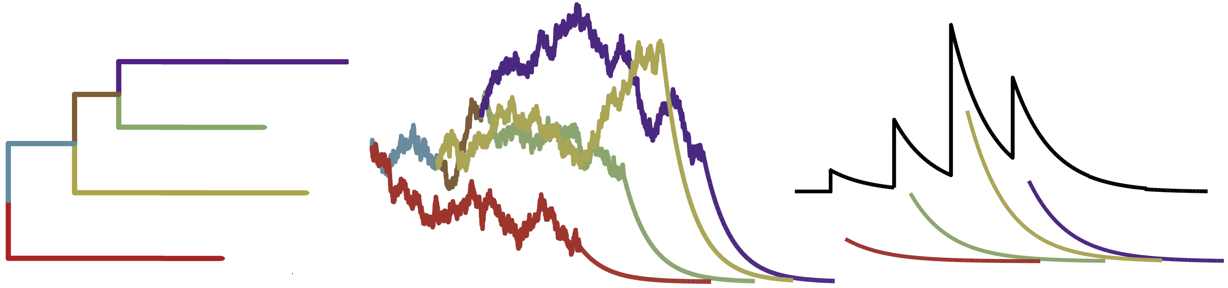
Figure 1: The phylogenetic Hawkes process relates the evolutionary history of a virus to the rate at which subsequent viral cases occur nearby. Left: a phylogenetic tree characterizes the evolution of a viral strain. Middle: a Brownian motion ‘along the tree’ describes the evolution of infinitesimal rates as a function of branch lengths and tree topology (Section 2.2). Right: virus-specific rates additively contribute to the rate of occurrence for future cases (Section 2.1).

We use standard Bayesian phylogenetics hierarchical approaches (Suchard et al., 2003) to model a single molecular sequence alignment $\mathbf{S}$ containing sequences from $M\leq N$ evolutionarily related viruses. Let $\mathcal{M}$ denote the ordered index set with cardinality $|\mathcal{M}|=M$ containing every number within the set $\{1,\dots,N\}$ that corresponds to an observed virus for which genome data are present. In the following, we number the elements within $\mathcal{M}$ as $m_{1},m_{2},\dots,m_{M}$. Moreover, we make use of the set $\mathcal{M}^{+}$ with cardinality $|\mathcal{M}^{+}|=2M-1$, satisfying $\mathcal{M}\subset\mathcal{M}^{+}$ and containing elements $m_{1},\dots,m_{2M-1}$. Our primary object of interest is the phylogenetic tree ${\cal G}$ (Figure 1, left) defined as a bifurcating, directed graph with $M$ terminal degree-1 nodes $(\nu_{m_{1}},\ldots,\nu_{m_{M}})$ that correspond to the tips of the tree (or sequenced observations), $M-2$ internal degree-3 nodes $(\nu_{m_{M+1}},\ldots,\nu_{m_{2M-2}})$, a root degree-2 node $\nu_{m_{2M-1}}$ and edge weights $(w_{m_{1}},\ldots,w_{m_{2M-2}})$ that encode the elapsed evolutionary time between nodes. Here, each $w_{m}$ communicates the expected number of molecular substitutions per site, which is itself the product between the real time duration and the evolutionary rate arising from a molecular clock model. For example, we use a relaxed molecular clock model (Drummond et al., 2006b) that allows for substitution rates to flexibly vary accross branches (Section 3.2). One may either know ${\cal G}$ a priori or endow it with a prior distribution parameterized by some vector $\bm{\phi}$. Suchard et al. (2001) and Suchard et al. (2018) develop the joint distribution $p(\mathbf{S},\bm{\phi},{\cal G})$ in detail.

We assume that the event-specific rates $\bm{\theta}$ defined within our Hawkes model take the form (Figure 1, middle)

$$\begin{cases}\theta_{n}=\theta_{n}(z_{n})=\exp\left(z_{n}+\bm{\beta}^{T}\mathbf{f}(t_{n})\right)&z_{n}\in\mathbb{R}\,,\quad n\in\mathcal{M}\\ \theta_{n}=1&\quad n\notin\mathcal{M}\,,\\ \end{cases}$$

and that the elements of vector $\mathbf{z}=(z_{m_{1}},\dots,z_{m_{M}})^{T}$ follow a Brownian diffusion process along the branches of ${\cal G}$ (Cavalli-Sforza and Edwards, 1967; Felsenstein, 1985; Lemey et al., 2010). Here, $\mathbf{f}(\cdot)$ is some fixed vector function and the inclusion of the linear term $\bm{\beta}^{T}\mathbf{f}(t_{n})$ helps control for global trends resulting from extrinsic events such as mass quarantine or travel restrictions. Under the Brownian process, the latent value of a child node $\nu_{c}$ in tree ${\cal G}$ is normally distributed about the value of its parent node $\nu_{\text{\tiny pa}(c)}$ with variance $w_{c}\times\sigma^{2}$, where $\sigma^{2}$ gives the dispersal rate after controlling for correlation in values that are shared by descent through the phylogenetic tree ${\cal G}$. We further posit that the latent value of the root node $\nu_{m_{2M-1}}$ is a priori normally distributed with mean $0$ and variance $\tau_{0}\times\sigma^{2}$. The vector $\mathbf{z}$ is then multivariate normally distributed Cybis et al. (2015) and has probability density function

$$\small p(\mathbf{z}\,|\,\mathbf{V}_{{\cal G}},\sigma^{2},\tau_{0})=\left(2\pi\sigma^{2}\right)^{-M/2}\left|\mathbf{V}_{{\cal G}}\right|^{-1/2}\mbox{exp}\left(-\frac{1}{2\sigma^{2}}\mathbf{z}^{T}\mathbf{V}_{{\cal G}}^{-1}\mathbf{z}\right)\,,$$ (2)

where $\mathbf{V}_{{\cal G}}=\{v_{nm}\}$ is a symmetric, positive definite, block-diagonal $M\times M$ matrix with structure dictated by ${\cal G}$. Defining $d_{F}({u},{v})$ to be the sum of edge-weights along the shortest path between nodes $u$ and $v$ in tree ${\cal G}$, the diagonal elements $v_{mm}=\tau_{0}+d_{F}({\nu_{m_{2M-1}}},{\nu_{m_{m}}})$ are the elapsed evolutionary time between the root node and tip node $m_{m}$, and off-diagonal elements $v_{nm}=\tau_{0}+\left[d_{F}({\nu_{m_{2M-1}}},{\nu_{m_{n}}})+d_{F}({\nu_{m_{2M-1}}},{\nu_{m_{m}}})-d_{F}({\nu_{m_{n}}},{\nu_{m_{m}}})\right]/2$ are the evolutionary time period between the root node and the most recent common ancestor of tip nodes $m_{n}$ and $m_{m}$.

2.3 Inference

Due to the complexity of the phylogenetic Hawkes process and the large number of viruses we seek to model, we must use advanced statistical, algorithmic and computational tools to infer the posterior distribution

$$p(\sigma^{2},{\cal G},\bm{\phi},\mu_{0},\tau_{x},\theta_{0},\bm{\theta},\omega,h,\bm{\beta}\,|\,\mathbf{X},\mathbf{t},\mathbf{S})\propto \mathcal{L}(\mathbf{X},\mathbf{t}|\mu_{0},\tau_{x},\theta_{0},\bm{\theta}(\mathbf{z}),\omega,h)\times p(\mathbf{z}\,|\,\sigma^{2},{\cal G})\times$$ (3)

$$p(\mu_{0})\times p(\tau_{x})\times p(\theta_{0})\times p(\omega)\times p(h)\times p(\bm{\beta})\times$$

$$p(\sigma^{2})\times p(\mathbf{S},\bm{\phi},{\cal G})\,.$$

We do so using a random-scan Metropolis-with-Gibbs scheme, in which we compute key quantities with the help of adaptively preconditioned Hamiltonian Monte Carlo (HMC) (Neal, 2011), dynamic programming and parallel computing on cutting-edge graphics processing units (GPU).

2.3.1 Dynamic programming for phylogenetic diffusion quantities

We must evaluate $p(\mathbf{z}\,|\,\sigma^{2},{\cal G})$ to sample ${\cal G}$. The bottleneck within the evaluation of Equation (2) is the ostensibly ${\cal O}\left(M^{3}\right)$ matrix inverse $\mathbf{V}_{{\cal G}}^{-1}$, but Pybus et al. (2012) develop a dynamic programming algorithm to perform the requisite computations in ${\cal O}\left(M\right)$ with parallelized post-order traversals of ${\cal G}$. We use this algorithm, which is closely related to the linear-time algorithms of Freckleton (2012) and Ho and Ané (2014), as all are examples of message passing on a directed, acyclic graph (Cavalli-Sforza and Edwards, 1967; Pearl, 1982). Similar tricks render inference for $\bm{\phi}$ linear in $M$, and Fisher et al. (2021) extend Pybus et al. (2012) to compute gradients with respect to $\bm{\phi}$. Finally, implementing these algorithms on GPUs would lead to additional speedups (Suchard and Rambaut, 2009), but the computational bottleneck we face when applying the phylogenetic Hawkes process arises from the Hawkes process likelihood and its gradients.

2.3.2 Massive parallelization for Hawkes model quantities

Sampling the Hawkes process parameters $\mu_{0},\tau_{x},\theta_{0},\omega,h,\beta$ and event-specific rates $\bm{\theta}$ requires evaluation of the likelihood $\mathcal{L}(\mathbf{X},\mathbf{t}|\mu_{0},\tau_{x},\theta_{0},\bm{\theta},\omega,h)$ or its logarithm. Unfortunately, the double summation of Equation (1) results in an ${\cal O}\left(N^{2}\right)$ computational complexity that makes repeated likelihood evaluations all but impossible for the number of observations considered in this paper. We therefore use the high-performance computing framework of Holbrook et al. (2021) to massively parallelize likelihood evaluations in the context of univariate, adaptive Metropolis-Hastings proposals for parameters $\mu_{0},\tau_{x},\theta_{0},\omega$, $h$ and $\beta$. On the other hand, inference for the $M$-vector $\mathbf{z}$ requires more than fast univariate proposals, so we opt for HMC to sample from its high-dimensional posterior. Even in high dimensions, HMC efficiently generates proposal states by simulating a physical Hamiltonian system that renders the target posterior distribution invariant. Here, we follow standard procedure and specify the system with total energy

$$H(\mathbf{z},\mathbf{p})=-\log\big{(}\pi(\mathbf{z})\,\xi(\mathbf{p}|\mathbf{M})\big{)}\propto-\log\pi(\mathbf{z})+\frac{1}{2}\mathbf{p}^{T}\mathbf{M}^{-1}\mathbf{p}\,,$$

where $\pi(\mathbf{z})$ is the density of the marginal posterior for $\mathbf{z}$, $\mathbf{p}$ is a Gaussian distributed ‘momentum’ variable with density $\xi(\mathbf{p}|\mathbf{M})$, and $\mathbf{M}$ is the system mass matrix and the covariance of $\mathbf{p}$. We again follow standard HMC procedure and use the leapfrog algorithm (Leimkuhler and Reich, 2004) to integrate Hamilton’s equations

$$\dot{\mathbf{z}}=\frac{\partial}{\partial\mathbf{p}}H(\mathbf{z},\mathbf{p})=\frac{1}{2}\mathbf{M}^{-1}\mathbf{p}\,,\quad\dot{\mathbf{p}}=-\frac{\partial}{\partial\mathbf{z}}H(\mathbf{z},\mathbf{p})=\nabla\log\pi(\mathbf{z})\,.$$

But there is no free lunch: simulation of the physical system requires repeated evaluations of the log-likelihood gradient, and these evaluations may become burdensome in big data contexts. Indeed, the gradient of the Hawkes process log-likelihood of Equation (1) with respect to $\bm{\theta}$ becomes computationally onerous for large $N$ and $M$. The gradient with respect to a single event-specific rate $\theta_{m}$ takes the form

$$\frac{\partial\ell}{\partial\theta_{m}} =-\frac{\partial\Lambda_{m}}{\partial\theta_{m}}+\sum_{t_{m}<t_{n}}\frac{1}{\lambda_{n}}\frac{\partial\lambda_{nm}}{\partial\theta_{m}}$$ (4)

$$=\theta_{0}\left(e^{-\omega\,(t_{N}-t_{m})}-1\right)+\sum_{t_{m}<t_{n}}\frac{1}{\lambda_{n}}\frac{\theta_{0}\omega}{h^{D}}e^{-\omega\,(t_{n}-t_{m})}\phi\left(\frac{\mathbf{x}_{n}-\mathbf{x}_{m}}{h}\right)\,,$$

where the summation and $\lambda_{n}$ are both of complexity ${\cal O}\left(N\right)$. Thus, computing the entire vector $\partial\ell/\partial\bm{\theta}=(\partial\ell/\partial\theta_{1},\dots,\partial\ell/\partial\theta_{M})^{T}$ requires time ${\cal O}\left(NM\right)$. Worse still, due to the multiscale nature of the posterior for the relative rates (Figure 4), we find it necessary to precondition the Hamiltonian dynamics by specifying a diagonal mass matrix with elements

$$\mathbf{M}_{mm}^{-1}\approx-\frac{\partial^{2}\ell}{\partial\theta^{2}_{m}}=\sum_{t_{m}<t_{n}}\frac{1}{\lambda_{n}^{2}}\frac{\theta^{2}_{0}\omega^{2}}{h^{2D}}e^{-2\omega\,(t_{n}-t_{m})}\phi^{2}\left(\frac{\mathbf{x}_{n}-\mathbf{x}_{m}}{h}\right)\,.$$ (5)

Specifically, we maintain a running average of Hessians calculated at a fixed interval and use this as our preconditioner $\mathbf{M}$, thus maintaining asymptotic unbiasedness of Monte Carlo estimates (Haario et al., 2001). Just as with the gradient, the summation and $\lambda_{n}$ are both of complexity ${\cal O}\left(N\right)$, and the resulting complexity for the entire Hessian is ${\cal O}\left(NM\right)$. To overcome these rate-limiting steps, we develop massively parallel central processing unit (CPU) and GPU implementations of both the gradient and the Hessian. Although our GPU-based implementations are fastest (Section 3.1), our CPU implementations are competitive, making use of both multi-core processing and SIMD (single instruction, multiple data) vectorization (Holbrook et al., 2020). Regardless of implementation, all of our high-performance software remains freely available for public use.

2.4 Software availability

We use the Bayesian evolutionary analysis by sampling trees (BEAST) software package (Suchard et al., 2018), a popular tool for viral phylogenetic inference that implements MCMC methods to explore $p(\mathbf{S},\bm{\phi},{\cal G})$ and $p(\mathbf{z}\,|\,\sigma^{2},{\cal G})$ (Cybis et al., 2015) under a range of evolutionary models. In writing this paper, we have contributed to the open-source, stand-alone library hpHawkes http://github.com/suchard-group/hawkes for computing the spatiotemporal Hawkes process log-likelihood (Equation 1), its gradient (Equation 4) and its Hessian (Equation 5). hpHawkes integrates into BEAST with the help of an application programming interface (API). Within hpHawkes, we combine C++ code with which standard compilers generate vectorized CPU-specific instructions and OpenCL kernels that allow for GPU-specific optimization. Finally, we have used the Rcpp package (Eddelbuettel and François, 2011) to make the same massive parallelization speedups available to users of the R programming language.

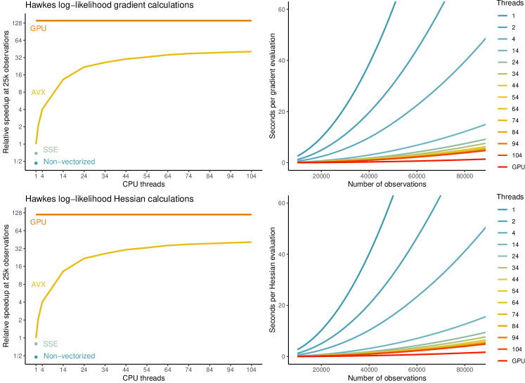
Figure 2: Spatiotemporal Hawkes process log-likelihood gradient and Hessian calculations with respect to event-specific rates $\bm{\theta}$ with central and graphics processing units (CPU and GPU). [Left] Multiplicative speedups over single-threaded advanced vector extensions (AVX) vectorization for single-threaded non-vectorized and streaming SIMD extensions (SSE), multi-threaded AVX and many-core GPU processing for 25,000 randomly generated data points. [Right] Seconds per gradient and Hessian calculations for multi-threaded AVX and GPU implementations from 10 to 90 thousand data points.

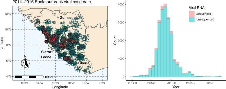
Figure 3: Spatiotemporal distribution of 23,178 viral cases during the 2014-2016 Ebola outbreak in Guinea, Sierra Leone and Liberia. Of this number, 1,367 viral samples yield RNA sequence data and interface directly with the prior over phylogenetic trees. All cases, both sequenced and unsequenced, interface with the Hawkes process likelihood.

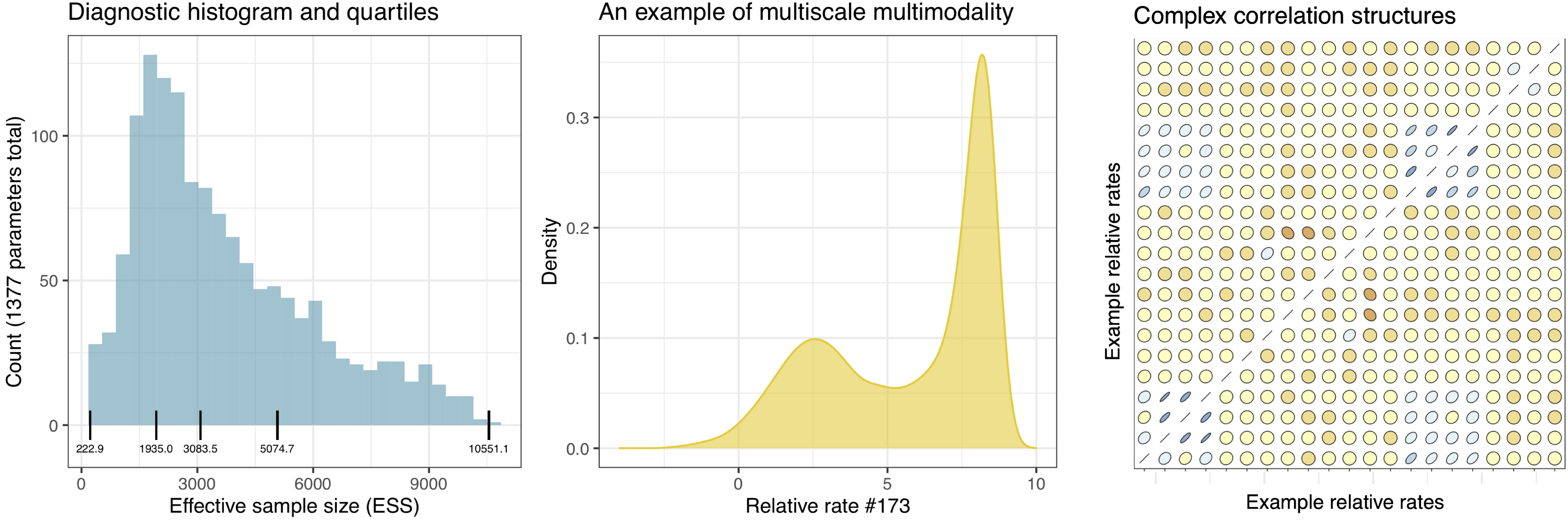
Figure 4: The posterior distribution presents multiple challenges: it is high-dimensional; it takes on different scales for different parameters; it is multimodal in some parameters; and it exhibits complex correlation structures between parameters. [Left] Histogram and quartiles from 100 million MCMC samples for the ESS of all 1377 model parameters. [Middle] Multimodal marginal posterior for a single relative rate. [Right] Posterior correlations between 21 relative rates.

3 Demonstration

3.1 Massive parallelization

Figure 2 shows benchmarking results for evaluating the Hawkes log-likelihood gradient with respect to event-specific rates $\bm{\theta}$ (Equation 4). For the GPU results, we use an NVIDIA Quadro GV100, which has 5,120 CUDA cores (at 1.13 GHz) and reaches an (unboosted) 2.9 teraflops peak double-precision floating point performance (or 5.8 teraflops for fused operations such as fused multiply-add). We use a Linux machine with two 26-core Intel Xeon Gold processors (2.1 GHz) for CPU results. Each physical core supports 2 threads or logical cores, and the machine achieves a peak performance of 874 gigaflops with double-precision floating point enhanced with AVX vectorization (again, double this for fused operations). Based on peak double-precision floating point operations, our a priori expectation is for fully parallelized GPU-based gradient evaluations to to be roughly 3.3 times faster than 104-threaded AVX evaluations on the CPU.

On the left of Figure 2, we compare relative efficiency for GPU and various CPU implementations of the log-likelihood gradient and Hessian for 25,000 simulated data points using single-threaded AVX computing (15.7 and 16.3 seconds per gradient and Hessian evaluations) as baseline. Using SSE or non-vectorized single-threaded computing results in 1.5- and 2.2-fold slowdowns for the gradient and 1.3- and 2.1-fold slowdowns for the Hessian. Sticking with AVX processing, we see diminishing returns as we increase the number of threads. For the both the gradient and the Hessian, the 14- 54- and 104-thread AVX implementations are roughly 13, 33 and 41 times faster than single-threaded AVX. Agreeing with our a priori expectations, the GPU implementation is 140.4 times faster than single-threaded AVX and 3.5 times faster than 104-threaded AVX for the gradient and 120.0 times faster than single-threaded AVX and 2.9 times faster than 104-threaded AVX for the Hessian. The right of Figure 2 demonstrates the ${\cal O}\left(N^{2}\right)$ computational complexity for the same gradient and Hessian evaluations by varying the number of data points from 10,000 to 90,000. While parallelization does not overcome this quadratic scaling, it does reduce computational costs for finite observation counts.

3.2 2014-2016 Ebola outbreak in West Africa

Hierarchical model			Posterior mean
module	Model parameter	Symbol	(95% HPD cred. int.)	Unit
Hawkes process	Background spatial lengthscale	$\tau_{x}$	194 (147, 243)	km
	Self-excitatory temporal lengthscale	$1/\omega$	29.8 (28.5, 30.9)	days
	Self-excitatory spatial lengthscale	$h$	7.37 (7.13, 7.62)	km
	Normalized self-excitatory weight	$\theta_{0}/(\theta_{0}+\mu_{0})$	0.96 (0.95, 0.97)	—
	Temporal trend coefficient	$\beta$	-2.22 (-2.37,-2.06)	—
Phylogenetic diffusion	Standard deviation	$\sigma$	51.0 (46.4, 55.7)	log rate

Table 2: Posterior means and 95% highest posterior density (HPD) credible intervals from the application of the phylogenetic Hawkes process to the 2014-2016 Ebola outbreak in Guinea, Sierra Leone and Liberia.

During the 2014-2016 outbreak in Guinea, Sierra Leone and Liberia, Ebola viral fever resulted in over 28,000 known cases and 11,000 known deaths (World Health Organization, 2015). First reports of the virus in Guinea emerged during March of 2014 (Baize et al., 2014). At around the same time, viral cases with the same Guinean origin (Gire et al., 2014) emerged in Sierra Leone and Liberia. In May 2014, the virus crossed from Guinea to Kailahun, Sierra Leone. From there, it spread to multiple counties of Liberia and Guinea (Dudas et al., 2017), and the same strain reached Freetown, the capital of Sierra Leone, by July 2014. In the fall of 2014, Sierra Leone and Liberia were detecting 500 and 700 new cases a week. Only by the end of 2014 did case numbers begin to abate in most areas due to control measures. By March of 2015 sustained transmission of the virus only continued in western Guinea and western Sierra Leone (Dudas et al., 2017). Figure 3 shows the spatiotemporal distribution of the majority of known Ebola virus cases during the epidemic.

Using our high performance computing framework, we apply the phylogenetic Hawkes process to the analysis of 23,422 viral cases. Dudas et al. (2017) provide a total of 1,610 cases furnishing genomic sequencing, 1,367 of which come with date and location data (https://github.com/ebov/space-time). We supplement this sequenced data with 21,811 date and location pairs from unsequenced cases documented by the World Health Organization (https://apps.who.int/gho/data/node.ebola-sitrep). The precision of the spatial data is district or county level. To leverage spatial information as much as practically possible within our Hawkes model, we assume the locations follow a Gaussian distribution at district population centroids and with variance guaranteeing a 95% probability of the case occurring within the circle of equal area to the district and centered at the population centroid. We then integrate over uncertainty with respect to these locations by periodically sampling new locations according to the assumed Gaussian distribution throughout the MCMC run and with a period of roughly 100 iterations. That said, sensitivity analyses show that model inference is robust to fixing randomly generated locations for the entire MCMC chain. We make the combined data and documentation for our entire BEAST analysis available within the single file Final.xml and place this as well as other project scripts together at the repository https://github.com/suchard-group/EBOVPhyloHawkes. In addition to the software mentioned in the previous section, we make use of the ggplot2 and ggmap R packages for data and results visualization (Wickham, 2016; Kahle and Wickham, 2013).

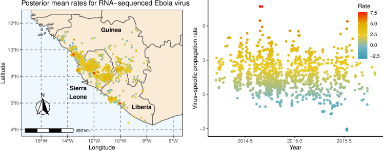
Figure 5: Hawkes model posterior mean rates $\bm{\theta}$ for the 1,367 (of 1,610) RNA-sequenced viral samples for which date/location data are available. Unsurprisingly, the largest relative rates occur within or nearby major clusters of events. Adjusting for downward trends in case data with a negative coefficient $\beta$ (Table 2) allows detection of higher relative rates after peak outbreak (late 2014) including a jump in infections mid-2015 (Figure 3).

For the phylogenetic prior specification $p(\mathbf{S},\bm{\phi},{\cal G})$, we follow the phylogeographic analysis of Dudas et al. (2017) and use a mixture of 1,000 phylogenetic trees obtained as high-probability posterior samples from their purely phylogenetic analysis of the 1,610 sequenced viral samples. In that preceding Bayesian analysis, Dudas et al. (2017) combine an HKY$+\Gamma_{4}$ substitution model prior for molecular evolution (Hasegawa et al., 1985; Yang, 1994), a relaxed molecular clock prior on rates (Drummond et al., 2006a), a non-parametric coalescent ‘Skygrid’ prior on effective population size dynamics (Gill et al., 2013) and a continuous time Markov chain reference prior for overall rate (Ferreira and Suchard, 2008). We assume a priori that the background lengthscale $\tau_{x}$ follows a diffuse inverse gamma distribution with shape 1 and scale 10, where distance units are latitudinal and longitudinal degrees. An inverse gamma distribution with shape and scale parameters equal to 2 and 0.5 for both $h$ and $1/\omega$ encodes our beliefs that self-excitatory dynamics occur at finer spatiotemporal scales, where years are the temporal units. We upweight self-excitatory dynamics by giving $\theta_{0}$ and $\mu_{0}$ gamma priors with shape parameters $1$ and $2$ and scale parameters $0.001$ and $2$, respectively. We absorb $\tau_{0}$ into $\sigma$ and place a tight inverse gamma prior on $1/\sigma$ with shape and scale parameters of 2 and 0.5. Finally, we set $\mathbf{f}(t_{n})=t_{n}$ and place a normal prior on the univariate coefficient $\beta$ with mean 0 and standard deviation of 10. We find all parameters robust to prior specification due to the large number of observations considered.

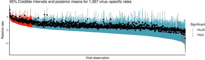
Figure 6: 95% credible intervals and posterior means for virus-specific rates $\bm{\theta}$ corresponding to the subset of 1,610 sequenced viruses that come with date/location data and therefore appear in the Hawkes process module. We call those 183 intervals which do not include 1 ‘significant’. Of these, 177 are above and 6 below 1. Appendix B has labels, locations and times for each.

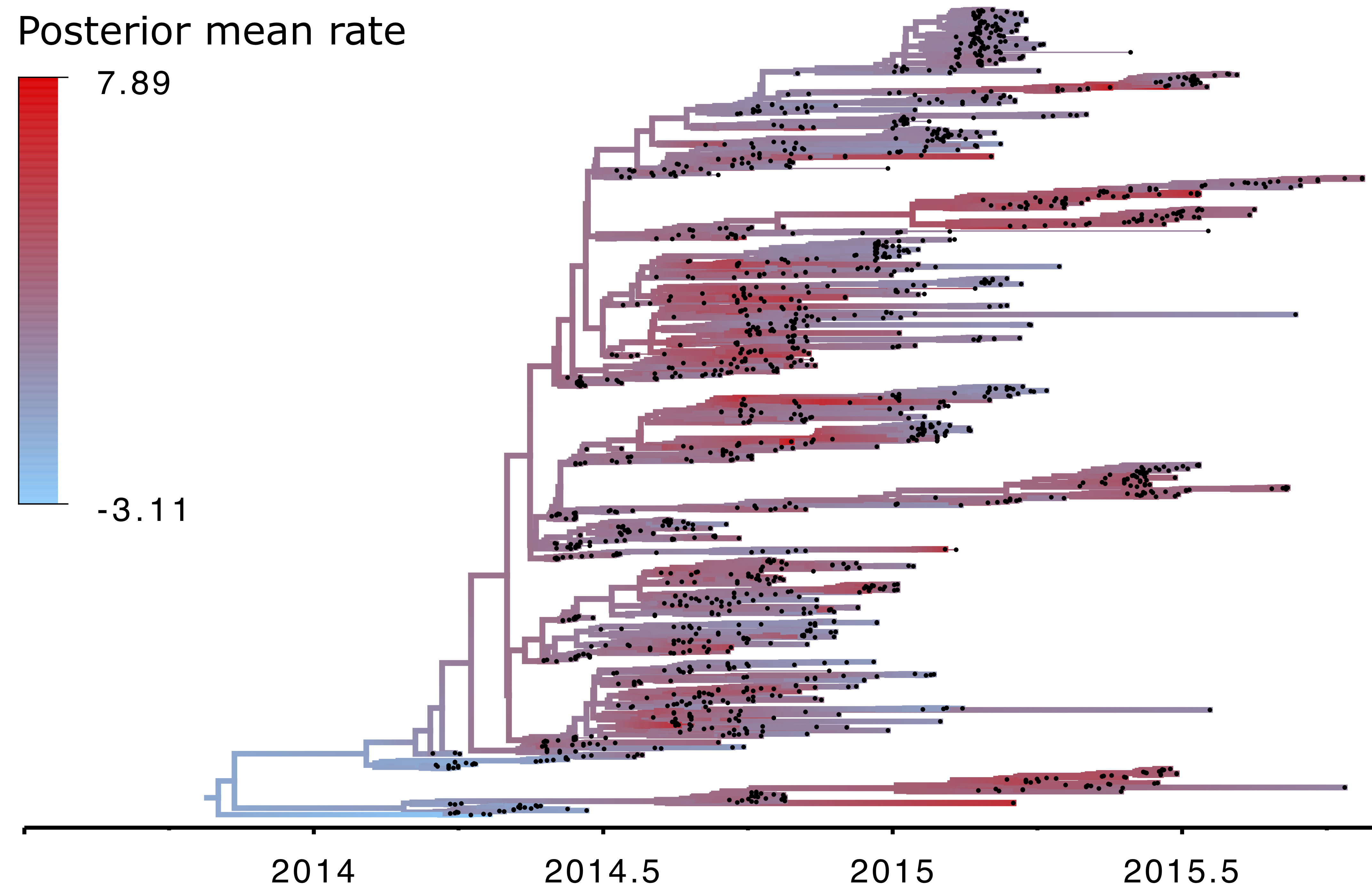
Figure 7: Posterior mean virus-specific relative rates color the posterior maximum clade credibility tree of phylogeny ${\cal G}$, a few subtrees of which potentially demonstrate elevated contagiousness.

We generate 100 million MCMC samples according to the routine outlined in Section 2.3 and discard the first 500 thousand as burn-in. Using our parallel computing algorithms and a single NVIDIA GV100 GPU (Section 3.1), the routine requires 6.77 hours to generate 1 million samples and 28 days to generate all 100 million samples. Figure 4 shows the distribution of effective samples sizes (ESS) across all model parameters and illustrates some of the challenges facing any MCMC routine for the phylognetic Hawkes model. Namely, the posterior distribution is high-dimensional, multimodal, multiscale and has complex correlation structures.

Table 2 shows posterior means and 95% highest posterior density (HPD) credible intervals for the phylogenetic Hawkes process parameters. The posterior mean for the spatial bandwidth $\tau_{x}$ of the Hawkes background process is 194 km (147, 243), allowing the model to incorporate and adapt to large scale geographic movement. On the other hand, the Hawkes process self-excitatory spatial bandwidth $h$ has a posterior mean of 7.4 km (7.1, 7.6), indicating the smaller local scale for which the model attributes viral contagion. The self-excitatory temporal bandwidth $1/\omega$ has a posterior mean of 29.8 days (28.5, 30.9), indicating the timescale for which the model attributes the same viral contagion. The normalized self-excitatory weight $\theta_{0}/(\theta_{0}+\mu_{0})$ indicates the proportion of events the model attributes to self-excitatory (compared to background) dynamics and has a posterior mean of 0.96 (0.95, 0.97). The posterior mean of the self-excitatory rate’s temporal trend coefficient $\beta$ is -2.22 (-2.37, -2.06) indicates that, for every additional year and ceteris paribus, one should expect a multiplicative decrease of $1-\exp(-2.22)\times 100\approx 90\%$ to the process self-excitatory rate. In this way, the model adjusts for downward trends arising from epidemiological control (e.g., mass quarantine and travel restrictions) and controls for these factors when inferring virus-specific relative rates.

Next, we consider posterior inference of the virus-specific rates $\bm{\theta}$ for those viral observations that provide RNA sequences. When interpreting these results, it is important to understand that the phylogenetic Hawkes process implicitly assumes that such samples spark nearby contagion as described by spatial and temporal bandwidths $h$ and $1/\omega$. Recall that the posteriors for these two parameters concentrate at over 7 km and 4 weeks, respectively. Figure 5 depicts the relationship between posterior mean values of $\bm{\theta}$ and the spatiotemporal distribution of corresponding viruses. Since these rates represent multiplicative factors of the global self-excitatory weight $\theta_{0}$, a null value would be 1. Posterior means range from approximately -2.5 to 7.5 and increasingly vary as a function of time. As one might expect, the highest rates appear near or within larger clusters. Thanks to the negative temporal trend coefficient $\beta$ and the increase of uncertainty with time, larger rate values do obtain for some viral cases occurring in 2015, despite following after peak epidemic. Figure 6 features posterior means and 95% intervals for the same virus-specific rates. Only a small subset of 183 rate intervals do not include 1. Of these, 177 have lower bound greater than 1, and 6 have upper bound below 1. We interpret all 103 of the corresponding viruses as having statistically significantly increased or decreased contagiousness. Virus-specific labels, locations and times for all 183 appear in Appendix B.

Finally, Figure 7 shows how these posterior rates organize as a function of the inferred posterior maximum clade credibility tree ${\cal G}$. Generally speaking, shorter branch lengths indicate larger effective populations of viruses, while larger branch lengths indicate smaller. For example, the structure of the bottom subtree reflects this intuition as branches are short with many splits during peak outbreak in the second half of 2014 but become mostly long in late 2014 and the remainder of 2015. According to the phylogenetic Brownian process model outlined in Section 2.2, virus-specific rate values are more highly correlated to one another when closely located to one-another on the the phylogenetic tree. It is plausible that these correlations allow the phylogenetic Hawkes model to infer higher rates for some strains that survive late into the epidemic despite dropping case counts. The model attributes some of the highest values to strains appearing in Coyah, Conakry and Kindia, Guinea, in late 2014 and early 2015. Interestingly, the model also attributes its lowest values to cases in Kono, Sierra Leone, in early 2015. Taken together, Figure 7 and the significant virus lists of Appendix B may provide helpful leads for epidemiologists searching for variants with heightened relative rates of contagion.

4 Discussion

We propose the phylogenetic Hawkes process, a Bayesian hierarchical model that relates viral spatial contagion to molecular evolution by uniting the two epidemiological paradigms of self-exciting point process and phylogenetic modeling. Due to difficulties in scaling the model to larger numbers of observations, we advance a computing strategy that combines HMC, dynamic programming and massive parallelization for key inferential bottlenecks. Finally, we apply our novel model and high performance computing framework to the analysis of over 23,000 viral cases arising from the 2014-2016 Ebola outbreak in West Africa, and Ebola strains and subtrees with plausibly higher degrees of contagiousness reveal themselves.

Unfortunately, the current model will fail when applied to the analysis of a global pandemic due to the dominant role of non-local, large scale transportation networks in propagating viral spread (Holbrook et al., 2020). We are particularly interested in developing extensions to the phylogenetic Hawkes process that leverage recent advances in scaling high-dimensional multivariate Hawkes processes (Nickel and Le, 2020) and applying the resulting multivariate phylogenetic Hawkes process to the analysis of global pandemics. In this context, each additional dimension will represent an additional country or province. Prodigious computational challenges are inevitable, and we suspect that non-trivial GPU implementations will be necessary for big data applications.

Moving beyond inference, a major question is whether the phylogenetic Hawkes process can be useful for prediction of spatial contagion and dynamics. Here, recent neural network extensions of the Hawkes process might prove useful (Mei and Eisner, 2017; Zuo et al., 2020; Zhang et al., 2020), but it is unclear what forward simulation of phylogenetic branching dynamics would look like in the context of a Hawkes process. Moreover, generating samples from the posterior predictive distribution of a Hawkes process would be extremely time consuming when one is conditioning on millions of posterior samples. To work around this, one could perhaps parallelize over fixed parameter settings the algorithm of Dassios and Zhao (2011) for simulating Hawkes processes when the temporal triggering function is exponential. Such an implementation would require efficient use of parallel pseudo-random number generators (Salmon et al., 2011).

Appendix A The likelihood integral with event-specific rates

Without loss of generality, we consider the temporal Hawkes process with constant background rate. To compute the likelihood (Equation 1), we must calculate the integral

$$\Lambda(t_{N}) =\int_{0}^{t_{N}}\lambda(t)\,\mbox{\emph{d}}t=\int_{0}^{t_{N}}\left(\mu+\theta_{0}\sum_{t_{n}<t}\theta_{n}\omega e^{-\omega\,(t-t_{n})}\right)\mbox{d}t$$

$$=\int_{0}^{t_{1}}\mu\,\mbox{d}t+\sum_{n=1}^{N-1}\int_{t_{n}}^{t_{n+1}}\left(\mu+\theta_{0}\sum_{t_{n}<t}\theta_{n}\omega e^{-\omega\,(t-t_{n})}\right)\mbox{d}t$$

$$=\mu\,t_{N}+\theta_{0}\omega\sum_{n=1}^{N-1}\int_{t_{n}}^{t_{n+1}}\sum_{n^{\prime}=1}^{n}\theta_{n^{\prime}}e^{-\omega\,(t-t_{n^{\prime}})}\,\mbox{d}t$$

$$=\mu\,t_{N}+\theta_{0}\omega\sum_{n=1}^{N-1}\sum_{n^{\prime}=1}^{n}\theta_{n^{\prime}}\int_{t_{n}}^{t_{n+1}}e^{-\omega\,(t-t_{n^{\prime}})}\,\mbox{d}t$$

$$=\mu\,t_{N}-\theta_{0}\sum_{n=1}^{N-1}\sum_{n^{\prime}=1}^{n}\theta_{n^{\prime}}\left(e^{-\omega\,(t_{n+1}-t_{n^{\prime}})}-e^{-\omega\,(t_{n}-t_{n^{\prime}})}\right)\,,$$

and we further simplify the double summation in the following.

Claim 1.

The temporal Hawkes process with rate function

$$\lambda(t)=\mu+\theta_{0}\sum_{t_{n}<t}\theta_{n}\omega e^{-\omega\,(t-t_{n})}$$ (6)

admits the integral

$$\Lambda(t_{N})=\int_{0}^{t_{N}}\lambda(t)\,\mbox{\emph{d}}t=\mu\,t_{N}-\theta_{0}\sum_{n=1}^{N-1}\theta_{n}\left(e^{-\omega(t_{N}-t_{n})}-1\right)\,.$$ (7)

Proof.

Proceeding by induction, the assertion is trivial for $N=1$. If it is true for some $N>0$, this implies that

$$\sum_{n=1}^{N-1}\sum_{n^{\prime}=1}^{n}\theta_{n^{\prime}}\left(e^{-\omega\,(t_{n+1}-t_{n^{\prime}})}-e^{-\omega\,(t_{n}-t_{n^{\prime}})}\right)=\sum_{n=1}^{N-1}\theta_{n}\left(e^{-\omega(t_{N}-t_{n})}-1\right)\,.$$

It follows that

$$\Lambda(t_{N+1}) =\mu\,t_{N+1}-\theta_{0}\sum_{n=1}^{N}\sum_{n^{\prime}=1}^{n}\theta_{n^{\prime}}\left(e^{-\omega\,(t_{n+1}-t_{n^{\prime}})}-e^{-\omega\,(t_{n}-t_{n^{\prime}})}\right)$$

$$=\mu\,(t_{N+1}-t_{N})-\theta_{0}\sum_{n^{\prime}=1}^{N}\theta_{n^{\prime}}\left(e^{-\omega\,(t_{N+1}-t_{n^{\prime}})}-e^{-\omega\,(t_{N}-t_{n^{\prime}})}\right)$$

$$\quad+\mu\,t_{N}-\theta_{0}\sum_{n=1}^{N-1}\sum_{n^{\prime}=1}^{n}\theta_{n^{\prime}}\left(e^{-\omega\,(t_{n+1}-t_{n^{\prime}})}-e^{-\omega\,(t_{n}-t_{n^{\prime}})}\right)$$

$$=\mu\,(t_{N+1}-t_{N})-\theta_{0}\sum_{n^{\prime}=1}^{N}\theta_{n^{\prime}}\left(e^{-\omega\,(t_{N+1}-t_{n^{\prime}})}-e^{-\omega\,(t_{N}-t_{n^{\prime}})}\right)+\Lambda(t_{n})$$

$$=\mu\,(t_{N+1}-t_{N})-\theta_{0}\sum_{n^{\prime}=1}^{N}\theta_{n^{\prime}}\left(e^{-\omega\,(t_{N+1}-t_{n^{\prime}})}-e^{-\omega\,(t_{N}-t_{n^{\prime}})}\right)$$

$$\quad+\mu\,t_{N}-\theta_{0}\sum_{n=1}^{N-1}\theta_{n}\left(e^{-\omega(t_{N}-t_{n})}-1\right)$$

$$=\mu\,t_{N+1}-\theta_{0}\sum_{n=1}^{N}\theta_{n}\left(e^{-\omega\,(t_{N+1}-t_{n})}-e^{-\omega\,(t_{N}-t_{n})}\right)$$

$$\quad-\theta_{0}\sum_{n=1}^{N-1}\theta_{n}\left(e^{-\omega(t_{N}-t_{n})}-1\right)$$

$$=\mu\,t_{N+1}-\theta_{0}\sum_{n=1}^{N}\theta_{n}\left(e^{-\omega\,(t_{N+1}-t_{n})}-1\right)\,,$$

thus completing the proof. ∎

Appendix B Viruses with statistically significant relative rates

The following observed viruses have relative rates for which the 95% credible intervals have lower bound greater than 1.

1EBOV|EM_COY_2015_013857||GIN|Forecariah|2015-03-182EBOV|EM_COY_2015_013731||GIN|Coyah|2015-03-143EBOV|EM_COY_2015_014261||GIN|Forecariah|2015-04-024EBOV|IPDPFHGINSP_GUI_2015_5339||GIN|Conakry|2015-04-085EBOV|KG12||GIN|Boke|2015-05-276EBOV|EM_COY_2015_017091||GIN|Boke|2015-05-287EBOV|EM_COY_2015_016483||GIN|Boke|2015-05-138EBOV|EM_COY_2015_016743||GIN|Boke|2015-05-199EBOV|KG88||GIN|Boke|2015-06-1910EBOV|KG90||GIN|Boke|2015-06-1911EBOV|KG87||GIN|Boke|2015-06-1912EBOV|KG80||GIN|Boke|2015-06-1813EBOV|KG35||GIN|Boke|2015-06-0814EBOV|GUI_CTS_2015_0052||GIN|Boke|2015-06-2515EBOV|GUI_CTS_2015_0050||GIN|Boke|2015-06-2016EBOV|GUI_CTS_2015_0051||GIN|Boke|2015-06-2117EBOV|KG91||GIN|Boke|2015-06-2018EBOV|KG45||GIN|Boke|2015-06-0919EBOV|EM_COY_2015_017574||GIN|Boke|2015-06-1020EBOV|IPDPFHGINSP_GUI_2015_6899||GIN|Boke|2015-05-1421EBOV|EM_COY_2015_014102||GIN|Conakry|2015-03-2622EBOV|IPDPFHGINSP_GUI_2015_4909||GIN|Conakry|2015-03-2923EBOV|IPDPFHGINSP_GUI_2015_5117||GIN|Dubreka|2015-04-0324EBOV|IPDPFHGINSP_GUI_2015_4786||GIN|Conakry|2015-03-2625EBOV|EM_COY_2015_014098||GIN|Conakry|2015-03-2626EBOV|EM_COY_2015_014100||GIN|Conakry|2015-03-2627EBOV|1648|KR534569|GIN|Kindia|2014-10-2328EBOV|20140174|KR653294|SLE|WesternUrban|2014-08-2729EBOV|20144521|KR653271|SLE|Kono|2014-11-1230EBOV|DML24511|KT357828|SLE|Kono|2015-01-1431EBOV|20146001|KR653237|SLE|Kono|2014-11-2432EBOV|20141352|KR653284|SLE|Kambia|2014-09-2633EBOV|G6069.1|KR105344|SLE|Kambia|2014-09-2534EBOV|20141997|KR653293|SLE|Kono|2014-10-1035EBOV|J0008|KP759718|SLE|WesternUrban|2014-09-2936EBOV|KT2449|KU296465|SLE|WesternUrban|2014-12-0537EBOV|20143458|KR653245|SLE|Tonkolili|2014-11-0138EBOV|J0016|KP759742|SLE|WesternRural|2014-09-3039EBOV|G6104.1|KR105349|SLE|Moyamba|2014-09-2840EBOV|20141397|KR653288|SLE|Moyamba|2014-09-2841EBOV|G6103.1|KR105348|SLE|Moyamba|2014-09-2842EBOV|PL6656|KU296523|SLE|PortLoko|2015-05-0143EBOV|PL7429|KU296617|SLE|PortLoko|2015-05-2944EBOV|PL7451|KU296837|SLE|PortLoko|2015-05-2945EBOV|PL7375|KU296498|SLE|PortLoko|2015-05-2746EBOV|PL7401|KU296819|SLE|PortLoko|2015-05-2747EBOV|G4725.1|KR105267|SLE|Moyamba|2014-08-0448EBOV|J0038|KP759618|SLE|PortLoko|2014-09-3049EBOV|J0102|KP759657|SLE|PortLoko|2014-10-2750EBOV|J0103|KP759658|SLE|PortLoko|2014-10-2951EBOV|J0104|KP759765|SLE|PortLoko|2014-10-2952EBOV|J0105|KP759766|SLE|PortLoko|2014-10-2953EBOV|20141282|KR653229|SLE|Kambia|2014-09-2354EBOV|J0027|KP759678|SLE|Bombali|2014-10-0255EBOV|G6091.1|KR105346|SLE|Tonkolili|2014-09-2756EBOV|J0162|KP759622|SLE|Kambia|2014-11-0957EBOV|J0034|KP759608|SLE|PortLoko|2014-09-3058EBOV|20141429|KR653260|SLE|Kono|2014-09-2859EBOV|G6089.1|KR105345|SLE|Tonkolili|2014-09-2760EBOV|G6095.1|KR105347|SLE|Tonkolili|2014-09-2761EBOV|20142551|KR653226|SLE|Koinadugu|2014-10-2362EBOV|20143648|KR653253|SLE|Koinadugu|2014-11-0363EBOV|20143938|KR653264|SLE|Koinadugu|2014-11-0764EBOV|20143659|KR653256|SLE|Koinadugu|2014-11-0365EBOV|20142895|KR653268|SLE|Koinadugu|2014-10-2466EBOV|20141271|KR653261|SLE|PortLoko|2014-09-2467EBOV|J0084|KP759753|SLE|PortLoko|2014-10-1668EBOV|J0083|KP759752|SLE|PortLoko|2014-10-1869EBOV|J0035|KP759609|SLE|PortLoko|2014-10-0170EBOV|J0058|KP759724|SLE|PortLoko|2014-10-0871EBOV|J0071|KP759736|SLE|PortLoko|2014-10-0972EBOV|20140024|KR653252|SLE|PortLoko|2014-08-2073EBOV|G4972.1|KR105285|SLE|Kenema|2014-08-1474EBOV|20140433|KR653246|SLE|Tonkolili|2014-09-0375EBOV|J0030|KP759606|SLE|PortLoko|2014-10-0376EBOV|J0011|KP759641|SLE|PortLoko|2014-09-2977EBOV|20141288|KR653232|SLE|PortLoko|2014-09-2378EBOV|J0013|KP759643|SLE|PortLoko|2014-09-2879EBOV|J0014|KP759740|SLE|PortLoko|2014-09-2980EBOV|J0114|KP759596|SLE|PortLoko|2014-10-2981EBOV|J0115|KP759597|SLE|PortLoko|2014-10-2982EBOV|G4956.1|KR105282|SLE|Tonkolili|2014-08-1383EBOV|20140134|KR653227|SLE|Bombali|2014-08-2684EBOV|J0020|KP759755|SLE|Bombali|2014-09-2585EBOV|J0019|KP759754|SLE|Bombali|2014-09-2586EBOV|J0022|KP759757|SLE|Bombali|2014-09-2587EBOV|J0017|KP759747|SLE|Bombali|2014-09-2688EBOV|20142260|KR653262|SLE|Bombali|2014-10-1489EBOV|J0096|KP759654|SLE|WesternUrban|2014-10-2790EBOV|J0015|KP759741|SLE|Bombali|2014-09-2691EBOV|20141232|KR653266|SLE|Tonkolili|2014-09-2592EBOV|20142127|KR653234|SLE|Bombali|2014-10-1293EBOV|20141497|KR653273|SLE|Bombali|2014-10-0194EBOV|G5743.1|KR105323|SLE|Kono|2014-09-1795EBOV|G5529.1|KR105309|SLE|Kono|2014-09-0596EBOV|12854_EMLH|KU296729|SLE|WesternUrban|2015-04-1597EBOV|13031_EMLH|KU296665|SLE|WesternUrban|2015-05-1898EBOV|DML13828||SLE|WesternUrban|2015-06-2299EBOV|20143716|KR653292|SLE|Moyamba|2014-11-04100EBOV|20144610|KR653270|SLE|Tonkolili|2014-11-12101EBOV|J0021|KP759756|SLE|Bombali|2014-09-29102EBOV|PL5260|KU296591|SLE|Kambia|2015-03-23103EBOV|EM_COY_2015_013962||GIN|Forecariah|2015-03-22104EBOV|EM_COY_2015_013671||GIN|Coyah|2015-03-12105EBOV|PL4347|KU296720|SLE|Kambia|2015-03-04106EBOV|EM_COY_2015_015815||GIN|Fria|2015-04-14107EBOV|IPDPFHGINSP_GUI_2015_5038||GIN|Conakry|2015-04-01108EBOV|EM_COY_2015_016414||GIN|Dubreka|2015-05-11109EBOV|EM_COY_2015_017865||GIN|Dubreka|2015-06-18110EBOV|REDC-GUI-2015-00502||GIN|Conakry|2015-07-13111EBOV|REDC_GUI_2015_00483||GIN|Conakry|2015-07-12112EBOV|REDC-GUI-2015-00402||GIN|Conakry|2015-07-08113EBOV|EM_COY_2015_017057||GIN|Dubreka|2015-05-27114EBOV|EM_COY_2015_017135||GIN|Dubreka|2015-05-29115EBOV|EM_COY_2015_016800||GIN|Dubreka|2015-05-20116EBOV|EM_COY_2015_016617||GIN|Dubreka|2015-05-16117EBOV|EM_COY_2015_016531||GIN|Dubreka|2015-05-14118EBOV|PL4094|KU296476|SLE|Kambia|2015-02-27119EBOV|14795_EMLK|KU296737|SLE|Kambia|2015-04-25120EBOV|EM_COY_2015_014370||GIN|Forecariah|2015-04-07121EBOV|EM_COY_2015_013795||GIN|Forecariah|2015-03-16122EBOV|LIBR10106|KT725337|LBR|Nimba|2014-08-20123EBOV|LIBR10081|KT725339|LBR|Margibi|2014-08-26124EBOV|LIBR10017|KT725293|LBR|Montserrado|2014-08-19125EBOV|LIBR10170|KT725350|LBR|Montserrado|2014-08-17126EBOV|CDC-NIH-257||LBR|Montserrado|2014-08-27127EBOV|LIBR10082|KT725300|LBR|Margibi|2014-08-26128EBOV|LIBR10029|KT725348|LBR|Margibi|2014-08-16129EBOV|LIBR10030|KT725257|LBR|Margibi|2014-08-16130EBOV|LIBR10025|KT725315|LBR|Margibi|2014-08-16131EBOV|LIBR10088|KT725349|LBR|Montserrado|2014-08-26132EBOV|LIBR10087|KT725346|LBR|Margibi|2014-08-26133EBOV|LIBR10086|KT725381|LBR|Margibi|2014-08-26134EBOV|EM_075368|KR817131|GIN|Macenta|2014-08-29135EBOV|EM_000015|KR817067|GIN|Macenta|2014-09-01136EBOV|EM_000321|KR817074|GIN|Macenta|2014-09-09137EBOV|EM_074785|KR817126|GIN|Macenta|2014-08-16138EBOV|EM_000218|KR817072|GIN|Macenta|2014-09-07139EBOV|EM_000127|KR817070|GIN|Gueckedou|2014-09-04140EBOV|EM_000028|KR817069|GIN|Macenta|2014-09-01141EBOV|EM_000502|KR817078|GIN|Macenta|2014-09-13142EBOV|EM_001102|KR817089|GIN|Lola|2014-10-05143EBOV|Conakry_645|KR534513|GIN|Macenta|2014-08-14144EBOV|EM_074548|KR817123|LBR|Lofa|2014-08-08145EBOV|EM_078416|KR817161|GIN|Faranah|2014-11-24146EBOV|EM_078415|KR817160|GIN|Faranah|2014-11-24147EBOV|EM_075447|KR817134|GIN|Macenta|2014-08-31148EBOV|EM_075373|KR817132|GIN|Macenta|2014-08-30149EBOV|789|KR534523|GIN|Dubreka|2014-08-29150EBOV|1622|KR534567|GIN|Nzerekore|2014-10-22151EBOV|EM_075435|KR817133|GIN|Kerouane|2014-08-30152EBOV|EM_004201|KR817093|GIN|Kissidougou|2014-12-24153EBOV|EM_004259|KR817094|GIN|Kissidougou|2014-12-26154EBOV|EM_004290|KR817095|GIN|Kissidougou|2014-12-27155EBOV|EM_078722|KR817175|GIN|Kissidougou|2014-12-16156EBOV|EM_078779|KR817177|GIN|Kissidougou|2014-12-18157EBOV|EM_078694|KR817171|GIN|Kissidougou|2014-12-14158EBOV|EM_004059|KR817090|GIN|Kissidougou|2014-12-20159EBOV|EM_078706|KR817173|GIN|Kissidougou|2014-12-15160EBOV|EM_004085|KR817091|GIN|Kissidougou|2014-12-19161EBOV|EM_078763|KR817176|GIN|Kissidougou|2014-12-17162EBOV|LIBR0284|KT725328|LBR|GrandCapeMount|2014-11-22163EBOV|CDC-NIH-3832||LBR|GrandCapeMount|2014-11-23164EBOV|LIBR0286|KR006952|LBR|GrandCapeMount|2014-11-22165EBOV|LIBR10103|KT725338|LBR|Nimba|2014-08-20166EBOV|LIBR10035|KT725259|LBR|GrandBassa|2014-08-15167EBOV|EM_074438|KR817118|GIN|Nzerekore|2014-08-01168EBOV|EM_000706|KR817079|GIN|Nzerekore|2014-09-21169EBOV|EM_074439|KR817119|GIN|Nzerekore|2014-08-01170EBOV|EM_074436|KR817116|GIN|Nzerekore|2014-08-01171EBOV|EM_074437|KR817117|GIN|Nzerekore|2014-08-01172EBOV|LIBR10127|KT725272|LBR|Bong|2014-08-22173EBOV|LIBR0071|KT725303|LBR|GrandBassa|2014-11-06174EBOV|LIBR0059|KR006941|LBR|RiverCess|2014-11-05175EBOV|LIBR0058|KR006940|LBR|RiverCess|2014-11-05176EBOV|EM095|KM034550|SLE|Kailahun|2014-05-25177EBOV|G3676|KM034554|SLE|Kailahun|2014-05-27

The following observed viruses have relative rates for which the 95% credible intervals have upper bound less than 1.

1EBOV|EM_079413|KR817184|GIN|Gueckedou|2014-03-312EBOV|EM_079414|KR817185|GIN|Gueckedou|2014-03-313EBOV|EM_079542|KR817199|GIN|Gueckedou|2014-04-124EBOV|EM_079578|KR817201|GIN|Gueckedou|2014-04-185EBOV|EM_079587|KR817202|GIN|Gueckedou|2014-04-226EBOV|EM_079514|KR817197|GIN|Gueckedou|2014-04-10

Appendix C Parallelized gradient algorithms

Algorithms 1 and 2 present instructions for computing the Hawkes process log-likelihood gradient (Equation 4) with respect to the $M$-vector $\bm{\theta}$ of event-specific rates. Figure 2 shows resulting speedups for both Algorithm (1) and Algorithm (2) on a CPU and GPU, respectively.

Algorithm 1 Parallel evaluation of Hawkes process log-likelihood gradient:
Makes use of multiple central processing unit (CPU) cores and loop vectorization to calculate Hawkes process log-likelihood gradient with respect to event-specific rates $\bm{\theta}$. When using double-precision floating point, this algorithm may use either SSE or AVX vectorization to make $J=2$- or $4$-long jumps. We denote the number of CPU cores as $B$. Symbols $\ell$, $\lambda$ and $\Lambda$ appear in Equations (1) and (4).

1:Compute rates $\lambda_{1},\dots,\lambda_{N}$:

2:a:     parfor $b\in\{1,\dots,B\}$ do

3:b:        if $b\neq B$ then

4:c:          $Upper\leftarrow b\lfloor N/B\rfloor$

5:d:        else

6:e:           $Upper\leftarrow\lceil N/B\rceil$

7:f:        end if

8:g:        for $n\in\{(b-1)\lfloor N/B\rfloor+1,\dots,Upper\}$ do

9:h:           copy $\mathbf{x}_{n}$, $t_{n}$ to cache

10:i:           $\bm{\lambda}_{n}\leftarrow\mathbf{0}$ $\triangleright$ vector of length J

11:j:           $n^{\prime}\leftarrow 1$

12:k:           while $n^{\prime}<N$ do

13:l:              $J\leftarrow\min(J,N-n^{\prime})$

14:m:              copy $\mathbf{x}_{n^{\prime}:(n^{\prime}+J)}$, $t_{n^{\prime}:(n^{\prime}+J)}$ to cache

15:n:              $\bm{\Delta}_{nn^{\prime}}:\bm{\Delta}_{nn^{\prime}:(n^{\prime}+J-1)}\leftarrow(\mathbf{x}_{n}-\mathbf{x}_{n^{\prime}}):(\mathbf{x}_{n}-\mathbf{x}_{n^{\prime}+J-1})$ $\triangleright$ vectorized subtraction

16:o:              calculate $\delta_{nn^{\prime}}:\delta_{n(n^{\prime}+J-1)}$ $\triangleright$ vectorized multiplication

17:p:              calculate $\lambda_{nn^{\prime}}:\lambda_{n(n^{\prime}+J-1)}$ $\triangleright$ vectorized evaluation

18:q:              $\bm{\lambda}_{n}\leftarrow\bm{\lambda}_{n}+\lambda_{nn^{\prime}}:\lambda_{n(n^{\prime}+J-1)}$ $\triangleright$ vectorized addition

19:r:              $n^{\prime}\leftarrow n^{\prime}+J$

20:s:           end while

21:t:        end for

22:u:     end parfor

23:Compute $M$ gradients $\frac{\partial\ell}{\partial\theta_{n}}$:

24:a:     parfor $b\in\{1,\dots,B\}$ do

25:b:        if $b\neq B$ then

26:c:          $Upper\leftarrow b\lfloor M/B\rfloor$

27:d:        else

28:e:           $Upper\leftarrow\lceil M/B\rceil$

29:f:        end if

30:g:        for $n\in\{(b-1)\lfloor M/B\rfloor+1,\dots,Upper\}$ do

31:h:           copy $\mathbf{x}_{n}$, $t_{n}$ to cache

32:i:           $\frac{\partial\ell}{\partial\theta_{n}}\leftarrow 0$

33:j:           $n^{\prime}\leftarrow 1$

34:k:           while $n^{\prime}<N$ do

35:l:              $J\leftarrow\min(J,N-n^{\prime})$

36:m:              copy $\mathbf{x}_{n^{\prime}:(n^{\prime}+J)}$, $t_{n^{\prime}:(n^{\prime}+J)}$ to cache

37:n:              $\bm{\Delta}_{nn^{\prime}}:\bm{\Delta}_{nn^{\prime}:(n^{\prime}+J-1)}\leftarrow(\mathbf{x}_{n}-\mathbf{x}_{n^{\prime}}):(\mathbf{x}_{n}-\mathbf{x}_{n^{\prime}+J-1})$ $\triangleright$ vectorized subtraction

38:o:              calculate $\delta_{nn^{\prime}}:\delta_{n(n^{\prime}+J-1)}$ $\triangleright$ vectorized multiplication

39:p:              calculate $e^{-\omega\,(t_{n^{\prime}}-t_{n})}\phi\left(\frac{\delta_{nn^{\prime}}}{h}\right):e^{-\omega\,(t_{n^{\prime}+J-1}-t_{n})}\phi\left(\frac{\delta_{n(n^{\prime}+J-1)}}{h}\right)$ $\triangleright$ vectorized evaluation

40:q:              for $j\in{n^{\prime},\dots,n^{\prime}+J-1}$ do

41:r:                 $\frac{\partial\ell}{\partial\theta_{n}}\leftarrow\frac{\partial\ell}{\partial\theta_{n}}+\mathcal{I}_{[t_{n}<t_{j}]}\frac{1}{\lambda_{j}}\frac{\partial\lambda_{jn}}{\partial\theta_{n}}$

42:s:              end for

43:t:              $n^{\prime}\leftarrow n^{\prime}+J$

44:u:           end while

45:v:        $\frac{\partial\ell}{\partial\theta_{n}}\leftarrow\frac{\partial\ell}{\partial\theta_{n}}+\theta_{0}\left(e^{-\omega\,(t_{N}-t_{n})}-1\right)$

46:w:        end for

47:x:     end parfor

Algorithm 2 Parallel evaluation of Hawkes process log-likelihood gradient:
Computes the log-likelihood gradient with respect to event-specific rates $\bm{\theta}$ using multiple levels of parallelization on a graphics processing unit (GPU). In this paper, we specify $B=128$ for the size of the GPU work groups. Symbols $\ell$, $\lambda$ and $\Lambda$ appear in Equations (1) and (4).

1:Compute rates $\lambda_{1},\dots,\lambda_{N}$:

2:a:     parfor $n\in\{1,\dots,N\}$ do

3:b:        copy $\mathbf{x}_{n}$, $t_{n}$ to local $\triangleright$ $B$ threads

4:c:        parfor $N^{\prime}\in\{1,\dots,\lfloor N/B\rfloor\}$ do

5:d:           $n^{\prime}\leftarrow N^{\prime}$

6:e:           $\lambda_{nN^{\prime}}\leftarrow 0$

7:f:          while $n^{\prime}<N$ do

8:g:              copy $\mathbf{x}_{n^{\prime}}$, $t_{n^{\prime}}$ to local $\triangleright$ $B$ threads

9:h:              $\bm{\Delta}_{nn^{\prime}}\leftarrow\mathbf{x}_{n}-\mathbf{x}_{n^{\prime}}$ $\triangleright$ vectorized subtraction

10:i:              calculate $\delta_{nn^{\prime}}=\sqrt{\sum\bm{\Delta}_{nn^{\prime}}\circ\bm{\Delta}_{nn^{\prime}}}$ $\triangleright$ vectorized multiplication

11:j:              $\lambda_{nN^{\prime}}\leftarrow\lambda_{nN^{\prime}}+\lambda_{nn^{\prime}}$ $\triangleright$ $\lambda_{nn^{\prime}}$ a function of $\delta_{nn^{\prime}}$, $t_{n}$ and $t_{n^{\prime}}$

12:k:              $n^{\prime}\leftarrow n^{\prime}+B$

13:l:           end while

14:m:       end parfor

15:n:        $\lambda_{n}\leftarrow\sum_{N^{\prime}}\lambda_{nN^{\prime}}$ $\triangleright$ binary tree reduction on chip

16:o:     end parfor

17:Compute $M$ gradients $\frac{\partial\ell}{\partial\theta_{n}}$:

18:a:     parfor $n\in\{1,\dots,M\}$ do

19:b:        copy $\mathbf{x}_{n}$, $t_{n}$ to local $\triangleright$ $B$ threads

20:c:        parfor $N^{\prime}\in\{1,\dots,\lfloor N/B\rfloor\}$ do

21:d:           $n^{\prime}\leftarrow N^{\prime}$

22:e:           $\left(\frac{\partial\ell}{\partial\theta_{n}}\right)_{N^{\prime}}\leftarrow 0$

23:f:          while $n^{\prime}<N$ do

24:g:              copy $\mathbf{x}_{n^{\prime}}$, $t_{n^{\prime}}$ to local $\triangleright$ $B$ threads

25:h:              $\bm{\Delta}_{nn^{\prime}}\leftarrow\mathbf{x}_{n}-\mathbf{x}_{n^{\prime}}$ $\triangleright$ vectorized subtraction

26:i:              calculate $\delta_{nn^{\prime}}=\sqrt{\sum\bm{\Delta}_{nn^{\prime}}\circ\bm{\Delta}_{nn^{\prime}}}$ $\triangleright$ vectorized multiplication

27:j:              $\left(\frac{\partial\ell}{\partial\theta_{n}}\right)_{N^{\prime}}\leftarrow\left(\frac{\partial\ell}{\partial\theta_{n}}\right)_{N^{\prime}}+\mathcal{I}_{[t_{n}<t_{n^{\prime}}]}\frac{1}{\lambda_{n^{\prime}}}\frac{\partial\lambda_{n^{\prime}n}}{\partial\theta_{n}}$

28:k:              $n^{\prime}\leftarrow n^{\prime}+B$

29:l:           end while

30:m:       end parfor

31:n:        $\frac{\partial\ell}{\partial\theta_{n}}\leftarrow\sum_{N^{\prime}}\left(\frac{\partial\ell}{\partial\theta_{n}}\right)_{N^{\prime}}$ $\triangleright$ binary tree reduction on chip

32:o:        $\frac{\partial\ell}{\partial\theta_{n}}\leftarrow\frac{\partial\ell}{\partial\theta_{n}}+\theta_{0}\left(e^{-\omega\,(t_{N}-t_{n})}-1\right)$

33:p:     end parfor

References

- Bacry et al. (2015) Bacry, E., I. Mastromatteo, and J.-F. Muzy. 2015. Hawkes processes in finance. Market Microstructure and Liquidity 1:1550005.
- Baize et al. (2014) Baize, S., D. Pannetier, L. Oestereich, T. Rieger, L. Koivogui, N. Magassouba, B. Soropogui, M. S. Sow, S. Keïta, H. De Clerck, et al. 2014. Emergence of zaire ebola virus disease in guinea. New England Journal of Medicine 371:1418–1425.
- Bertozzi et al. (2020) Bertozzi, A. L., E. Franco, G. Mohler, M. B. Short, and D. Sledge. 2020. The challenges of modeling and forecasting the spread of covid-19. Proceedings of the National Academy of Sciences 117:16732–16738.
- Boni et al. (2020) Boni, M. F., P. Lemey, X. Jiang, T. T.-Y. Lam, B. W. Perry, T. A. Castoe, A. Rambaut, and D. L. Robertson. 2020. Evolutionary origins of the sars-cov-2 sarbecovirus lineage responsible for the covid-19 pandemic. Nature Microbiology 5:1408–1417.
- Brockmann and Helbing (2013) Brockmann, D. and D. Helbing. 2013. The hidden geometry of complex, network-driven contagion phenomena. science 342:1337–1342.
- Cavalli-Sforza and Edwards (1967) Cavalli-Sforza, L. L. and A. W. Edwards. 1967. Phylogenetic analysis. models and estimation procedures. American Journal of Human Genetics 19:233–257.
- Chiang et al. (2020) Chiang, W.-H., X. Liu, and G. Mohler. 2020. Hawkes process modeling of covid-19 with mobility leading indicators and spatial covariates. medRxiv .
- Cybis et al. (2015) Cybis, G., J. Sinsheimer, T. Bedford, A. Mather, P. Lemey, and M. Suchard. 2015. Assessing phenotypic correlation through the multivariate phylogenetic latent liability model. Annals of Applied Statistics 9:969 – 991.
- Daley and Jones (2003) Daley, D. J. and D. V. Jones. 2003. An Introduction to the Theory of Point Processes: Elementary Theory of Point Processes. Springer.
- Dassios and Zhao (2011) Dassios, A. and H. Zhao. 2011. A dynamic contagion process. Advances in applied probability 43:814–846.
- Drummond et al. (2006a) Drummond, A., S. Ho, M. Phillips, and A. Rambaut. 2006a. Relaxed phylogenetics and dating with confidence. PLoS Biology 4:e88.
- Drummond et al. (2006b) Drummond, A. J., S. Y. Ho, M. J. Phillips, and A. Rambaut. 2006b. Relaxed phylogenetics and dating with confidence. PLoS Biol 4:e88.
- Dudas et al. (2017) Dudas, G., L. M. Carvalho, T. Bedford, A. J. Tatem, G. Baele, N. R. Faria, D. J. Park, J. T. Ladner, A. Arias, D. Asogun, et al. 2017. Virus genomes reveal factors that spread and sustained the ebola epidemic. Nature 544:309–315.
- Eddelbuettel and François (2011) Eddelbuettel, D. and R. François. 2011. Rcpp: Seamless R and C++ integration. Journal of Statistical Software 40:1–18.
- Faria et al. (2014) Faria, N. R., A. Rambaut, M. A. Suchard, G. Baele, T. Bedford, M. J. Ward, A. J. Tatem, J. D. Sousa, N. Arinaminpathy, J. Pépin, et al. 2014. The early spread and epidemic ignition of hiv-1 in human populations. science 346:56–61.
- Felsenstein (1978) Felsenstein, J. 1978. The number of evolutionary trees. Systematic zoology 27:27–33.
- Felsenstein (1985) Felsenstein, J. 1985. Phylogenies and the comparative method. American Naturalist 125:1–15.
- Ferreira and Suchard (2008) Ferreira, M. A. and M. A. Suchard. 2008. Bayesian analysis of elapsed times in continuous-time markov chains. Canadian Journal of Statistics 36:355–368.
- Fisher et al. (2021) Fisher, A. A., X. Ji, Z. Zhang, P. Lemey, and M. A. Suchard. 2021. Relaxed random walks at scale. Systematic Biology .
- Fox et al. (2016) Fox, E. W., F. P. Schoenberg, J. S. Gordon, et al. 2016. Spatially inhomogeneous background rate estimators and uncertainty quantification for nonparametric hawkes point process models of earthquake occurrences. The Annals of Applied Statistics 10:1725–1756.
- Freckleton (2012) Freckleton, R. P. 2012. Fast likelihood calculations for comparative analyses. Methods in Ecology and Evolution 3:940–947.
- Gill et al. (2013) Gill, M. S., P. Lemey, N. R. Faria, A. Rambaut, B. Shapiro, and M. A. Suchard. 2013. Improving bayesian population dynamics inference: a coalescent-based model for multiple loci. Molecular biology and evolution 30:713–724.
- Gire et al. (2014) Gire, S. K., A. Goba, K. G. Andersen, R. S. Sealfon, D. J. Park, L. Kanneh, S. Jalloh, M. Momoh, M. Fullah, G. Dudas, et al. 2014. Genomic surveillance elucidates ebola virus origin and transmission during the 2014 outbreak. science 345:1369–1372.
- Haario et al. (2001) Haario, H., E. Saksman, J. Tamminen, et al. 2001. An adaptive metropolis algorithm. Bernoulli 7:223–242.
- Habbema et al. (1974) Habbema, J., H. JDF, K. Van den Broek, et al. 1974. A stepwise discriminant analysis program using density estimation. .
- Hasegawa et al. (1985) Hasegawa, M., H. Kishino, and T.-a. Yano. 1985. Dating of the human-ape splitting by a molecular clock of mitochondrial dna. Journal of molecular evolution 22:160–174.
- Hawkes (1972) Hawkes, A. 1972. Spectra of some mutually exciting point processes with associated variables. Stochastic point processes Pages 261–271.
- Hawkes (1973) Hawkes, A. 1973. Cluster models for earthquakes-regional comparisons. Bull. Int. Stat. Inst. 45:454–461.
- Hawkes (1971a) Hawkes, A. G. 1971a. Point spectra of some mutually exciting point processes. Journal of the Royal Statistical Society: Series B (Methodological) 33:438–443.
- Hawkes (1971b) Hawkes, A. G. 1971b. Spectra of some self-exciting and mutually exciting point processes. Biometrika 58:83–90.
- Hawkes (2018) Hawkes, A. G. 2018. Hawkes processes and their applications to finance: a review. Quantitative Finance 18:193–198.
- Ho and Ané (2014) Ho, L. S. T. and C. Ané. 2014. A linear-time algorithm for Gaussian and non-Gaussian trait evolution models. Systematic Biology 3:397–402.
- Holbrook et al. (2020) Holbrook, A. J., P. Lemey, G. Baele, S. Dellicour, D. Brockmann, A. Rambaut, and M. A. Suchard. 2020. Massive parallelization boosts big bayesian multidimensional scaling. Journal of Computational and Graphical Statistics Pages 1–34.
- Holbrook et al. (2021) Holbrook, A. J., C. E. Loeffler, S. R. Flaxman, and M. A. Suchard. 2021. Scalable bayesian inference for self-excitatory stochastic processes applied to big american gunfire data. Statistics and Computing 31:1–15.
- Kahle and Wickham (2013) Kahle, D. and H. Wickham. 2013. ggmap: Spatial visualization with ggplot2. The R journal 5:144–161.
- Kelly et al. (2019) Kelly, J. D., J. Park, R. J. Harrigan, N. A. Hoff, S. D. Lee, R. Wannier, B. Selo, M. Mossoko, B. Njoloko, E. Okitolonda-Wemakoy, et al. 2019. Real-time predictions of the 2018–2019 ebola virus disease outbreak in the democratic republic of the congo using hawkes point process models. Epidemics 28:100354.
- Kim (2011) Kim, H. 2011. Spatio-temporal point process models for the spread of avian influenza virus (H5N1). Ph.D. thesis UC Berkeley.
- Kobayashi and Lambiotte (2016) Kobayashi, R. and R. Lambiotte. 2016. Tideh: Time-dependent hawkes process for predicting retweet dynamics. in Proceedings of the International AAAI Conference on Web and Social Media vol. 10.
- Leimkuhler and Reich (2004) Leimkuhler, B. and S. Reich. 2004. Simulating Hamiltonian dynamics vol. 14. Cambridge university press.
- Lemey et al. (2009) Lemey, P., A. Rambaut, A. Drummond, and M. Suchard. 2009. Bayesian phylogeography finds its roots. PLoS Computational Biology 5:e1000520.
- Lemey et al. (2010) Lemey, P., A. Rambaut, J. Welch, and M. Suchard. 2010. Phylogeography takes a relaxed random walk in continuous space and time. Molecular Biology and Evolution 27:1877–1885.
- Loeffler and Flaxman (2018) Loeffler, C. and S. Flaxman. 2018. Is gun violence contagious? a spatiotemporal test. Journal of quantitative criminology 34:999–1017.
- Mau et al. (1999) Mau, B., M. A. Newton, and B. Larget. 1999. Bayesian phylogenetic inference via markov chain monte carlo methods. Biometrics 55:1–12.
- Mei and Eisner (2017) Mei, H. and J. M. Eisner. 2017. The neural Hawkes process: A neurally self-modulating multivariate point process. Pages 6754–6764 in Advances in Neural Information Processing Systems.
- Meyer et al. (2014) Meyer, S., L. Held, et al. 2014. Power-law models for infectious disease spread. The Annals of Applied Statistics 8:1612–1639.
- Mohler (2014) Mohler, G. 2014. Marked point process hotspot maps for homicide and gun crime prediction in chicago. International Journal of Forecasting 30:491–497.
- Mohler et al. (2013) Mohler, G. et al. 2013. Modeling and estimation of multi-source clustering in crime and security data. The Annals of Applied Statistics 7:1525–1539.
- Neal (2011) Neal, R. M. 2011. MCMC using Hamiltonian dynamics. Handbook of Markov Chain Monte Carlo 2.
- Nickel and Le (2020) Nickel, M. and M. Le. 2020. Learning multivariate hawkes processes at scale. arXiv preprint arXiv:2002.12501 .
- Ogata (1988) Ogata, Y. 1988. Statistical models for earthquake occurrences and residual analysis for point processes. Journal of the American Statistical association 83:9–27.
- Park et al. (2019) Park, J., F. P. Schoenberg, A. L. Bertozzi, and P. J. Brantingham. 2019. Investigating clustering and violence interruption in gang-related violent crime data using spatial-temporal point processes with covariates .
- Pearl (1982) Pearl, J. 1982. Reverend Bayes on inference engines: A distributed hierarchical approach. Pages 133–136 in AAAI-82: Proceedings of the Second National Conference on Artificial Intelligence.
- Pybus et al. (2012) Pybus, O. G., M. A. Suchard, P. Lemey, F. J. Bernardin, A. Rambaut, F. W. Crawford, R. R. Gray, N. Arinaminpathy, S. L. Stramer, M. P. Busch, et al. 2012. Unifying the spatial epidemiology and molecular evolution of emerging epidemics. Proceedings of the National Academy of Sciences 109:15066–15071.
- Rambaut et al. (2008) Rambaut, A., O. G. Pybus, M. I. Nelson, C. Viboud, J. K. Taubenberger, and E. C. Holmes. 2008. The genomic and epidemiological dynamics of human influenza a virus. Nature 453:615–619.
- Reinhart (2018) Reinhart, A. 2018. A review of self-exciting spatio-temporal point processes and their applications. Statistical Science 33:299–318.
- Rizoiu et al. (2017) Rizoiu, M.-A., Y. Lee, S. Mishra, and L. Xie. 2017. A tutorial on hawkes processes for events in social media. arXiv preprint arXiv:1708.06401 .
- Rizoiu et al. (2018) Rizoiu, M.-A., S. Mishra, Q. Kong, M. Carman, and L. Xie. 2018. Sir-Hawkes: Linking epidemic models and Hawkes processes to model diffusions in finite populations. Pages 419–428 in Proceedings of the 2018 World Wide Web Conference on World Wide Web International World Wide Web Conferences Steering Committee.
- Robert (1976) Robert, P. 1976. On the choice of smoothing parameters for parzen estimators of probability density functions. IEEE Transactions on Computers 25:1175–1179.
- Ronquist et al. (2012) Ronquist, F., M. Teslenko, P. Van Der Mark, D. L. Ayres, A. Darling, S. Höhna, B. Larget, L. Liu, M. A. Suchard, and J. P. Huelsenbeck. 2012. Mrbayes 3.2: efficient bayesian phylogenetic inference and model choice across a large model space. Systematic biology 61:539–542.
- Salmon et al. (2011) Salmon, J. K., M. A. Moraes, R. O. Dror, and D. E. Shaw. 2011. Parallel random numbers: as easy as 1, 2, 3. Pages 1–12 in Proceedings of 2011 International Conference for High Performance Computing, Networking, Storage and Analysis.
- Schoenberg (2004) Schoenberg, F. P. 2004. Testing separability in spatial-temporal marked point processes. Biometrics Pages 471–481.
- Schoenberg (2013) Schoenberg, F. P. 2013. Facilitated estimation of etas. Bulletin of the Seismological Society of America 103:601–605.
- Schoenberg (2020) Schoenberg, F. P. 2020. Nonparametric estimation of variable productivity hawkes processes. arXiv preprint arXiv:2003.08858 .
- Schoenberg et al. (2019) Schoenberg, F. P., M. Hoffmann, and R. J. Harrigan. 2019. A recursive point process model for infectious diseases. Annals of the Institute of Statistical Mathematics 71:1271–1287.
- Sinsheimer et al. (1996) Sinsheimer, J. S., J. A. Lake, and R. J. Little. 1996. Bayesian hypothesis testing of four-taxon topologies using molecular sequence data. Biometrics Pages 193–210.
- Smith et al. (2009) Smith, G. J., D. Vijaykrishna, J. Bahl, S. J. Lycett, M. Worobey, O. G. Pybus, S. K. Ma, C. L. Cheung, J. Raghwani, S. Bhatt, et al. 2009. Origins and evolutionary genomics of the 2009 swine-origin h1n1 influenza a epidemic. Nature 459:1122–1125.
- Suchard et al. (2003) Suchard, M., C. Kitchen, J. Sinsheimer, and R. Weiss. 2003. Hierarchical phylogenetic models for analyzing multipartite sequence data. Systematic Biology 52:649–664.
- Suchard and Rambaut (2009) Suchard, M. and A. Rambaut. 2009. Many-core algorithms for statistical phylogenetics. Bioinformatics 25:1370–1376.
- Suchard et al. (2001) Suchard, M., R. Weiss, and J. Sinsheimer. 2001. Bayesian selection of continuous-time Markov chain evolutionary models. Molecular Biology and Evolution 18:1001–1013.
- Suchard et al. (2018) Suchard, M. A., P. Lemey, G. Baele, D. L. Ayres, A. J. Drummond, and A. Rambaut. 2018. Bayesian phylogenetic and phylodynamic data integration using BEAST 1.10. Virus Evolution 4:vey016.
- Wadman (2021) Wadman, M. 2021. United states rushes to fill void in viral sequencing. Science (New York, NY) 371:657–658.
- Wickham (2016) Wickham, H. 2016. ggplot2: Elegant Graphics for Data Analysis. Springer-Verlag New York.
- World Health Organization (2015) World Health Organization. 2015. Who: Ebola situation report 30 december 2015 .
- Yang (1994) Yang, Z. 1994. Maximum likelihood phylogenetic estimation from dna sequences with variable rates over sites: approximate methods. Journal of Molecular evolution 39:306–314.
- Yang and Rannala (1997) Yang, Z. and B. Rannala. 1997. Bayesian phylogenetic inference using dna sequences: a markov chain monte carlo method. Molecular biology and evolution 14:717–724.
- Yuan et al. (2021) Yuan, B., F. Schoenberg, and A. Bertozzi. 2021. Fast estimation of multivariate spatiotemporal hawkes processes and network reconstruction. Annals of the Institute of Statistical Mathematics Pages 1–26.
- Zhang et al. (2020) Zhang, Q., A. Lipani, O. Kirnap, and E. Yilmaz. 2020. Self-attentive hawkes process. Pages 11183–11193 in International Conference on Machine Learning PMLR.
- Zhuang et al. (2004) Zhuang, J., Y. Ogata, and D. Vere-Jones. 2004. Analyzing earthquake clustering features by using stochastic reconstruction. Journal of Geophysical Research: Solid Earth 109.
- Zuo et al. (2020) Zuo, S., H. Jiang, Z. Li, T. Zhao, and H. Zha. 2020. Transformer hawkes process. Pages 11692–11702 in International Conference on Machine Learning PMLR.