Revisiting Priority $k$-Center: Fairness and Outliers

Abstract

In the Priority $k$-Center problem, the input consists of a metric space $(X,d)$, an integer $k$ and for each point $v\in X$ a priority radius $r(v)>0$. The goal is to choose $k$ centers $S\subseteq X$ to minimize $\max_{v\in X}\frac{1}{r(v)}d(v,S)$. If all $r(v)$’s are uniform, one obtains the $k$-Center problem. Plesník [33] introduced the Priority $k$-Center problem and gave a $2$-approximation algorithm matching the best possible algorithm for $k$-Center. We show how the Priority $k$-Center problem is related to two different notions of fair clustering [26, 28]. Motivated by these developments we revisit the problem and, in our main technical contribution, develop a framework that yields constant factor approximation algorithms for Priority $k$-Center with outliers. Our framework extends to generalizations of Priority $k$-Center to matroid and knapsack constraints, and as a corollary, also yields algorithms with fairness guarantees in the lottery model of Harris et al. [24].

1 Introduction

Clustering is a basic task in a variety of areas, and clustering problems are ubiquitous in practice, and are well-studied in algorithms and discrete optimization. Recently fairness has become an important concern as automated data analysis and decision making have become increasingly prevalent in society. This has motivated several problems in fair clustering and associated algorithmic challenges. In this paper, we show that two different fairness views are inherently connected with a previously studied clustering problem called the Priority $k$-Center problem.

The input to Priority $k$-Center is a metric space $(X,d)$ and a priority radius $r(v)>0$ for each $v\in X$. The objective is to choose $k$ centers $S\subseteq X$ such that $\max_{v\in X}\frac{d(v,S)}{r(v)}$ is minimized. If one imagines clients located at each point in $X$, and $r(v)$ is the “speed” of a client at point $v$, then the objective is to open $k$ centers so that every client can reach an open center as quickly as possible. When all the $r(v)$’s are the same, then one obtains the classic $k$-Center problem [27, 21]. Plesník [33] introduced the Priority $k$-Center problem under the name of Weighted $k$-Center; the name Priority $k$-Center was given by Gørtz and Wirth [22] and this is what we use. Plesník [33] generalized Hochbaum and Shmoys’ [27] $2$-approximation algorithm for the $k$-Center problem and obtained the same bound for Priority $k$-Center. This approximation ratio is tight since $(2-\varepsilon)$-factor approximation is ruled out even for the classic $k$-Center problem under the assumption that $P\neq NP$ [25].

Connections to Fair Clustering. Our motivation to revisit Priority $k$-Center comes from two recent papers that considered fair variants in clustering, without explicitly realizing the connection to Priority $k$-Center. One of them is the paper of Jung, Kannan, and Lutz [28] who defined a version of fair clustering as follows. Given $(X,d)$ representing clients/people in a geographic area, and an integer $k$, for each $v\in X$ let $r_{\ell}(v)$ denote the smallest radius $r$ such that there are at least $\ell$ points of $X$ inside a ball of radius $r$ around $v$. They suggested a notion of fair $k$-Center as one in which each point $v\in X$ should be served by a center not farther than $r(v)=r_{n/k}(v)$ since the average size of a cluster in a clustering with $k$ clusters is $n/k$.  [28] describe an algorithm that finds $k$ centers such that each point $v$ is served by a center at most distance $2r_{n/k}(v)$ away from $v$. Once the radii are fixed for the points, then one obtains an instance of Priority $k$-Center, and their result essentially follows from the algorithm in [33]; indeed, the algorithm in [28] is the same.

Another notion of fairness related to the Priority $k$-Center is the lottery model introduced by Harris et al. [24]. In this model, every client $v\in X$ has a “probability demand” $\textsf{prob}(v)$ and a “distance demand” $r(v)$. Letting $\mathcal{S}$ denote all subsets of $k$ centers, their objective is to find a distribution over $\mathcal{S}$ such that for every client $v\in X$, $\Pr_{S\sim\mathcal{S}}[d(v,S)\leq r(v)]\geq\textsf{prob}(v)$. An $\alpha$-approximate algorithm will either prove such a solution is not possible, or provide a distribution where the distance to $S$ can be relaxed to $\alpha\cdot r(v)$, i.e. $\Pr_{S\sim\mathcal{S}}[d(v,S)\leq\alpha\cdot r(v)]\geq\textsf{prob}(v)$. Using a standard reduction via the Ellipsoid method [17, 1], this boils down to the outlier version of Priority $k$-Center, where some points in $X$ are allowed to be discarded. The outlier version of Priority $k$-Center had not been explicitly studied before.

Our Contributions. Motivated by these connections to fairness, we study the natural generalizations of Priority $k$-Center that have been studied for the classical $k$-center problem. The main generalization is the outlier version of Priority $k$-Center: the algorithm is allowed to discard a certain number of points when evaluating the quality of the centers chosen. First, the outlier version arises in the lottery model of fairness. Second, in many situations it is useful and important to discard outliers to obtain a better solution. Finally, it is also interesting from a theoretical point of view. We also consider the situation when the constraint on where centers can be opened is more general than the cardinality constraint. In particular, we study the Priority Matroid Center problem where the set of centers must be an independent set of a given matroid, and the Priority Knapsack Center problem where the total weight of centers opened is at most a certain amount. Our main contribution is an algorithmic framework to study the outlier problems in all these variations.

1.1 Statement of Results

We briefly describe some variants of Priority $k$-Center. In the Priority $k$-Supplier problem, the point space $X=F\uplus C$, and the goal is to select $k$ facilities $S\subseteq F$ to minimize $\max_{v\in C}d(v,S)/r(v)$. In the Priority Matroid Supplier problem, the subset of facilities needs to be an independent set of a matroid defined over $F$. In the Priority Knapsack Supplier problem, each facility has a weight, and the total weight of the subset of facilities opened must be at most a certain given bound. When all $r(v)$’s are the same, each of these problems admit a $3$-approximation [27, 13]. Our first result is that these results can be extended to the setting where the $r(v)$’s can be different. Furthermore, we establish the approximation bounds via standard LP-relaxations for the problems. Consequently, this can be used to re-derive and extend the algorithmic results in  [28]; we provide details of this in  Section 6.

Result 1.

There is a $3$-approximation for the Priority $k$-Supplier, Priority Matroid Supplier, and Priority Knapsack Supplier problems.

Our second, and main technical contribution, is a general framework to handle outliers for priority center problems. Given an instance of Priority $k$-Center and an integer $m\leq n$, the outlier version that we refer to as P$k$CO, is to find $k$ centers $S$ and a set $C^{\prime}$ of at least $m$ points from $C$ such that $\max_{v\in C^{\prime}}\frac{1}{r(v)}d(v,S)$ is minimized. While the $k$-Center with outliers admits a clever, yet relatively simple, greedy $3$-approximation due to Charikar et al. [11], a similar approach seems difficult to adapt for Priority $k$-Center with outliers. Instead, we take a more general and powerful LP-based approach from [9, 15] to develop a framework to handle P$k$CO, and also the outlier version of Priority Matroid Center (PMCO), where the opened centers must be an independent set of a matroid, and Priority Knapsack Center (PKnapCO), where the total weight of the open centers must fit in a budget. We obtain the following results.

Result 2.

There is a $9$-approximation for P$k$CO and PMCO and a $14$-approximation for PKnapCO. Moreover, the approximation ratio for P$k$CO and PMCO are with respect to a natural LP relaxation.

At this point we remark that a result in Harris et al. [24] (Theorem 2.8 in the arXiv version) also indirectly gives a $9$-approximation for P$k$CO. We believe that our framework is more general and is able to handle PMCO and PKnapCO easily. [24] does not consider these versions, and for the PKnapCO problem, their framework cannot give a constant factor approximation since they (in essence) use a weak LP relaxation.

Furthermore, our framework yields better approximation factors when either the number of distinct priorities are small, or they are at different scales. In practice, one probably expects this to be the case. In particular, when there are only two distinct types of radii, we obtain a $3$-approximation which is tight; it is not too hard to show that it is NP-hard to obtain a better than $3$-approximation for P$k$CO with two types of priorities. Interestingly, when there is a single priority, the $k$-Center with Outliers has a $2$-approximation [9] showing a gap between the two problems. More details are discussed in Remark 9. We obtain $5$- and $7$-approximate solutions when the number of radii are three and four, respectively. If all the different priority values are powers of $b$ (for some parameter $b>1$), we can derive a $\frac{3b-1}{b-1}$-approximation. Thus, if all the priorities are in vastly different scales ($b\to\infty$), then our approximation factor approaches $3$.

A summary of our results can be found in the third column of Table 1.

Result 3.

Suppose there are only two distinct priority radii among the clients. Then there is a $3$-approximation for P$k$CO, PMCO and PKnapCO. With $t$ distinct types of priorities, the approximation factor for P$k$CO and PMCO is $2t-1$. If all distinct types are powers of $b$, the approximation factor for P$k$CO and PMCO becomes $(3b-1)/(b-1)$.

It is possible that the P$k$CO problem (without any restrictions) has a $3$-approximation, and even the natural LP-relaxation may suffice; we have not been able to obtain a worse than $3$ integrality gap example. Resolving the integrality gap of the natural LP-relaxation and/or obtaining improved approximation ratios are interesting open questions highlighted by our work.

Remark 1.

Our results in Sections Sections 3, 4 and 5 are for Priority Center with Outliers problems. Our framework is able to handle the corresponding Priority Supplier with Outliers problems. We discuss the changes needed when handling the supplier versions in Appendix C.

Consequences for Fair Clustering. The algorithm in [28] is made much more transparent by the connection to Priority $k$-Center. Since Priority $k$-Center is more general, it allows one to refine and generalize the constraints that one can impose in the clustering model and use LP relaxations to find more effective solutions in particular scenarios. In addition, by allowing outliers, one can find tradeoffs between the quality of the solution and the number of points served. We provide more details in Section 6.

Recall the lottery model of Harris et al. [24] which we discussed previously. The algorithm in [24] is based on a sophisticated dependent rounding scheme and analysis. In fact, we observe that implicit in their result is a $9$-approximation for P$k$CO modulo some technical details. We can ask whether the result in [24] extends to the more general setting of Matroid Center and Knapsack Center. We prove that an $\alpha$-approximation algorithm for weighted outliers can be translated, via the Ellipsoid method, to yield the results in the probabilistic model of [24]. This is not surprising since a very similar reduction was shown in [1] in the context of the Colorful $k$-Center problem with outliers. The advantage of this black box reduction is evident from our algorithm from PKnapCO, which is non-trivial and is based on dynamic programming and on the round-or-cut approach since the natural LP has an unbounded integrality gap. It is not at all obvious how one can directly round a fractional solution to the problem while the generic transformation is clean and simple at the high level. For instance, our $3$-approximation for two radii extends to the lottery model immediately.

Table 1: Traditional vs. Priority Center Approximation Results

Problem	Traditional	Priority
$k$-Center	2 [27]	2 [33, 28], (Theorem 2)
$k$-Supplier	3 [27]	3 (Theorem 3)
Knapsack Supplier	3 [27]	3 (Theorem 3)
Matroid Supplier	3 [13]	3 (Theorem 3)
$k$-Center with Outliers	2 [9]	9 (Theorem 4)
Matroid Center with Outliers	3 [26, 15]	9 (Theorem 12)
Knapsack Center with Outliers	3 [15]	14 (Theorem 18)

1.2 Technical Discussion

Many clustering algorithms for the $k$-Center objective use a partitioning subroutine due to Hochbaum and Shmoys [27] (HS, henceforth). This procedure returns a partition $\Pi$ of $X$ along with a representative for each part such that all vertices of a part “piggy-back” on the representative. More precisely, if the representative is assigned to a center $f\in X$, then so are all other vertices in that part. To ensure a good algorithm for the $k$-Center problem, it suffices to ensure that the radius of each part is small.

For the Priority $k$-Center objective, one needs to be more careful: to use the above idea, one needs to make sure that if vertex $v$ is piggybacking on vertex $u$, then $r(v)$ better be more than $r(u)$. Indeed, this can be guaranteed by running the HS procedure in a particular order, namely by allowing vertices with smaller $r(v)$ to form the parts first. This is precisely Plesník’s algorithm [33]. In fact, this idea easily gives a $3$-approximation for the Matroid and Supplier versions as well.

Outliers are challenging in the setting of Priority $k$-Center. We start with the approach of Chakrabarty et al. [9] for $k$-Center with Outliers. First, they construct an LP where $\textsf{cov}(v)$ denotes the fractional coverage (amount to which one is not an outlier) of any point, and then write a natural LP for it. They show that if the HS algorithm is run according to the $\textsf{cov}(v)$ order (higher coverage vertices first), then the resulting partition can be used to obtain a $2$-approximation for the $k$-Center with Outliers problem.

When one moves to the priority $k$-Center with Outliers, one sees the obvious trouble: what if the $r(v)$ order and the $\textsf{cov}(v)$ order are at loggerheads? Our approach out of this is a simple bucketing idea. We first write a natural LP with fractional coverages $\textsf{cov}(v)$ for every point. Then, we partition vertices into classes: all vertices $v$ with $r(v)$ between $2^{i}$ and $2^{i+1}$ are in the same class. We then use the HS partitioning algorithm in the decreasing $\textsf{cov}(v)$ order separately on each class. The issue now is to handle the interaction across classes. To handle this, we define a directed acyclic graph across these various partitions where representative $u$ has an edge to representative $v$ iff $d(u,v)$ is small ($\leq r(u)+r(v)$). It is a DAG because we point edges from higher $r(u)$ to the lower $r(v)$. Our main observation is that if we can peel out $k$ paths with “large value” (each representative’s value is how many points piggyback on it), then we can get a $9$-approximation for the priority $k$-center with outlier problem. We can show that a fractional solution of large value does exist using the fact that the DAG was constructed in a greedy fashion. Also, since the graph is a DAG, this LP is an integral min-cost max-flow LP. The factor $9$ arises out of a geometric series and bucketing. Indeed, when the radii are exact powers of $2$, we get a $5$-approximation, and when there are only two type of radii, we get a $3$-approximation which is tight.

The preceding framework can handle the PMCO and PKnapCO problems as well — recall that these are the Outlier versions of the Priority Matroid Center and Priority Knapsack Center problems, respectively. For PMCO, the flow problem is no longer a min-cost max-flow problem, but rather it reduces to a submodular flow problem which is solvable in polynomial time. Modulo this, the above framework gives a $9$-approximation. For PKnapCO, there are two issues. One is that the flow problem is no longer integral and solving the underlying optimization problem is likely to be NP-hard (we did not attempt a formal proof). Nevertheless, the framework has sufficient flexibility. The DAG can be converted to a rooted forest on which a dynamic programming (DP) algorithm can be employed to find the desired paths; relaxing the DAG to a rooted forest amounts to an increase in the approximation factor, yielding a $14$-approximate solution. However, a second issue that we face in PKnapCO is that a fractional solution to the natural LP does not suffice when using the DP-based algorithm on the forest; indeed the natural LP has an unbounded gap. This issue can be circumvented by employing the round-or-cut approach from [15]; either the DP on the rooted forest succeeds or we find a violated inequality for the large implicit LP that we use.

1.3 Other Related Works

There is a huge literature on clustering, and instead of summarizing the landscape, we mention a few works relevant to our paper. Gørtz and Wirth [22] study the asymmetric version of the Priorty $k$-Center problem, and prove that it is NP-hard to obtain any non-trivial approximation. A related problem to Priority $k$-Center is the Non-Uniform $k$-Center problem by Chakrabarty et al. [9], where instead of clients having radii bounds, the objective is to figure out centers of balls for different types of radii. Another related problem [19] is the Local $k$-Median problem where clients need to connect to facilities within a certain radius, but the objective is the sum instead of the max.

Fairness in clustering has also seen a lot of works recently. Apart from the two notions of fairness described above, which can be thought of as “individual fairness” guarantees, Chierichetti et al. [10] introduce the “group fairness” notion where points have color classes, and each cluster needs to contain similar proportion of colors as in the universe. Their results were generalized by a series of follow ups [34, 4, 3]. A similar concept for outliers led to the study of Fair Colorful $k$-Center. In this problem, the objective is to find $k$ centers which covers at least a prescribed number of points from each color class. This was introduced by Bandapadhyay et al. [5], and recently true approximation algorithms were concurrently obtained by Jia et al. [29] and Anegg et al. [1].

Another notion of fairness is introduced by Chen et al. [7] in which a solution is called fair if there is no facility and a group of at least $n/k$ clients, such that opening that facility lowers the cost of all members of the group. They give a $(1+\sqrt{2})$-approximation for $L_{1}$, $L_{2}$, and $L_{\infty}$ norm distances for the setting where facilities can be places anywhere in the real space. Recently Micha and Shah [31] showed that a modification of the same approach can give a close to $2$-approximation for $L_{2}$ case and proved $(1+\sqrt{2})$ factor is tight for $L_{1}$ and $L_{\infty}$.

Coming back to the model of Jung et al. [28], the local notion of neighborhood radius is also present in the metric embedding works of [6, 14] and were recently used by Mahabadi and Vakilian [32] to extend the results in [28] to other objectives such as $k$-Median and $k$-Means. The Priority $k$-Median problem was further studied [16, 35], with [35] providing currentlybest known approximation. Subsequently, Priority Matroid Median problem was studied by Bajpai and Chekuri [2]. The outlier versions of these problems are an open direction of study.

2 Preliminaries

We provide some formal definitions and describe a clustering routine from [27].

Definition 1 (Priority $k$-Center).

The input is a metric space $(X,d)$. We are also given a radius function $r:X\to\mathbb{R}^{+}$, and integer $k$. The goal is to find $S\subseteq X$ of size at most $k$ to minimize $\alpha$ such that for all $v\in X$, $d(v,S)\leq\alpha\cdot r(v)$.

The following problem is an abstract generalization of the Priority $k$-Center problem, and is inspired by the corresponding generalization of $k$-Center from [15]. This problem will be convenient when describing certain parts of our framework.

Definition 2 (Priority $\mathscr{F}$-Supplier).

The input is a metric space $(X,d)$ where $X=F\cup C$, $C$ is the set of clients, and $F$ the set of facilities. We are also given a radius function $r:C\to\mathbb{R}^{+}$. The goal is to find $S\subseteq F$ to minimize $\alpha$ such that for all $v\in C$, $d(v,S)\leq\alpha\cdot r(v)$. The constraint on $F$ is that it must be selected from a down-ward closed family $\mathscr{F}$. Different families lead to different problems. We obtain the Priority $k$-Supplier problem if $\mathscr{F}=\{S\subseteq F\mid|S|\leq k\}$. We obtain the Priority Matroid Supplier problem when $(F,\mathscr{F})$ is a matroid. We obtain the Priority Knapsack Supplier problem when there is a weight function $w:F\to\mathbb{R}_{\geq 0}$ and $\mathscr{F}=\{S\subseteq F\mid w(S)\leq B\}$ for some budget $B$; here $w(S)$ denotes $\sum_{u\in S}w(u)$.

For the remainder of this manuscript, we focus on the feasibility version of the problem. More precisely, given an instance of the problem, we either want to show there is no solution with $\alpha=1$, or find a solution with $\alpha\leq\rho$. If we succeed, then via binary search we derive a $\rho$-approximation.

Plesník [33] obtained a $2$-approximation for Priority $k$-Center by running a procedure similar to that of Hochbaum and Shmoys [27], but where points are chosen in order of priorities ([27] uses an arbitrary order). Algorithm 1 is a slight generalization of this approach; in addition to the radius function and the metric, it takes as input a function $\phi:X\to R_{\geq 0}$ which encodes an ordering over the points (we can think of the points as being ordered from largest to smallest $\phi$ values). As previously mentioned, this algorithm is a similar procedure to that of [27], but while [27] picks points arbitrarily and [33] picks in order of priorities, points here get picked in the order mandated by $\phi$. Going forward, we use $r_{u}$ to denote $r(u)$ for convenience.

Algorithm 1 Filter

1:Metric $(X,d)$, radius function $r:X\to\mathbb{R}_{>0}$, and ordering $\phi:X\to\mathbb{R}_{\geq 0}$

2:$U\leftarrow X$ $\triangleright$ The set of uncovered points

3:$S\leftarrow\emptyset$ $\triangleright$ The set of “representatives”

4:while  $U\neq\emptyset$ do

5:     $u\leftarrow\arg\max_{v\in U}\phi(v)$ $\triangleright$ The first point in $U$ in non-increasing $\phi$ order

6:     $S\leftarrow S\cup u$

7:     $D(u)\leftarrow\{v\in U:d(u,v)\leq r_{u}+r_{v}\}$$\triangleright$ Note: $D(u)$ includes $u$ itself

8:     $U\leftarrow U\backslash D(u)$

9:end while

10:$S$, $\{D(u):u\in S\}$

We begin with a few straightforward observations about the output of Filter.

Fact 1.

The following is true for the output of Filter: (a) $\forall u,v\in S,d(u,v)>r_{u}+r_{v}$, (b) The set $\{D(u):u\in S\}$ partitions $X$, (c) $\forall{u\in S},\forall{v\in D(u)},\phi(u)\geq\phi(v)$, and (d) $\forall{u\in S},\forall{v\in D(u)},d(u,v)\leq r_{u}+r_{v}$.

Suppose we set $\phi(u):=1/r_{u}$ for each $u\in X$; we obtain Plesník’s algorithm and this yields a $2$-approximate solution for Priority $k$-Center. For completeness and later use we give a proof.

Theorem 2.

[33] There is a $2$-approximation for Priority $k$-Center.

Proof.

We claim that $S$, the output of Algorithm 1 for $\phi:=1/r$, is a 2-approximate solution; this follows from the observations in 1. For any $v\in X$ there is some $u\in S$ for which $v\in D(u)$. By our choice of $\phi$, $r_{u}\leq r_{v}$. Since $d(u,v)\leq r_{u}+r_{v}$, we have $d(u,v)\leq 2r_{v}$. To see why $|S|\leq k$, recall that for any $u,v\in S$, by 1, $d(u,v)>r_{u}+r_{v}$ so no two points in $S$ can be covered by the same center. Thus any feasible solution needs at least $|S|$ many points to cover all of $S$. ∎

In fact, under this setting of $\phi$, Algorithm 1 will almost immediately gives a $3$-approximation for Priority $\mathscr{F}$-Supplier for many families via the framework in [15], which we briefly describe.

The crux of the framework from [15] is that a solution to an $\mathscr{F}$-Supplier problem can be determined by selecting a “good” partition $\Pi$ of $F$ and determining whether $\Pi$ is “feasible” under $\mathscr{F}$. More formally, it requires efficient solvability of the following partition feasibility problem: given $\Pi$, is there an $A\in\mathscr{F}$ such that $|A\cap P|=1$ for all $P\in\Pi$? If no such $A$ exists, then the original instance is infeasible. If such an $A$ does exist, then the approximation quality of $A$ can be related to the goodness of $\Pi$.

For Priority $\mathscr{F}$-Supplier, consider the partition $P$ returned by Algorithm 1 using $\phi:=1/r$. Suppose we have partition feasibility oracle for $\mathscr{F}$ and it outputs a feasible $A$ for $P$. Then, by construction every $v\in X$ in part $D(u)$ satisfies $d(v,A)\leq d(u,v)+d(u,A)\leq 2r_{u}+r_{v}\leq 3r_{v}$ since $r_{u}\leq r_{v}$. Furthermore, one can see that if $\Pi$ is not feasible than the original instance is not feasible. For the Priority $k$-Supplier, Priority Matroid Center, and Priority Knapsack Center problems, the partition feasibility problem is solvable in polynomial time as shown in [15]. This leads to the following theorem.

Theorem 3.

There is a $3$-approximation for Priority $k$-Supplier, Priority Knapsack Center, and the Priority Matroid Center problem.

3 Priority $k$-Center with Outliers

In this section we describe our framework for handling priorities and outliers and give a $9$-approximation algorithm for the following problem.

Definition 3 (Priority $k$-Center with Outliers (P$k$CO)).

The input is a metric space $(X,d)$, a radius function $r:X\to\mathbb{R}_{>0}$, and parameters $k,m\in\mathbb{N}$. The goal is to find $S\subseteq X$ of size at most $k$ to minimize $\alpha$ such that for at least $m$ points $v\in X$, $d(v,S)\leq\alpha\cdot r(v)$.

Theorem 4.

There is a 9-approximation for P$k$CO.

The following is the natural LP relaxation for the feasibility version of P$k$CO. For each point $v\in X$, there is a variable $0\leq x_{v}\leq 1$ that denotes the (fractional) amount by which $v$ is opened as a center. We use $\textsf{cov}(v)$ to indicate the amount by which $v$ is covered by itself or other open facilities. To be precise, $\textsf{cov}(v)$ is the sum of $x_{u}$ over all $u\in X$ at distance at most $r_{v}$ from $v$. Note that $\textsf{cov}(v)$ is an auxiliary variable. We want to ensure that at least $m$ units of coverage are assigned using at most $k$ centers (hence the first two constraints).

$$\sum_{v\in X}\textsf{cov}(v) \geq m k$$ (PCO LP)

$$\sum_{v\in X}x_{v} \leq k$$

$$\textsf{cov}(v):=\sum_{\begin{subarray}{c}u\in X:\\ d(u,v)\leq r_{v}\end{subarray}}x_{u} \leq 1\qquad\forall v\in X$$

$$0\leq x_{v} \leq 1\qquad\forall v\in X.$$

Next, we define another problem called Weighted $k$-Path Packing (W$k$PP) on a DAG. Our approach is to do an LP-aware reduction from P$k$CO to W$k$PP. To be precise, we use a fractional solution of the P$k$CO LP to reduce to a W$k$PP instance $\mathcal{J}$. We show that a good integral solution for $\mathcal{J}$ translates to a $9$-approximate solution for the P$k$CO instance. We prove that $\mathcal{J}$ has a good integral solution by constructing a feasible fractional solution for an LP relaxation of W$k$PP; this LP relaxation is integral. Henceforth, $\mathcal{P}(G)$ denotes the set of all the paths in $G$ where each path is an ordered subset of the edges in $G$.

Definition 4 (Weighted $k$-Path Packing (W$k$PP)).

The input is $\mathcal{J}=\text{$(G=(V,E),\lambda,k)$}$ where $G$ is a DAG, $\lambda:V\rightarrow\{0,1,\dots,n\}$ for some integer $n$. The goal is to find a set of $k$ vertex disjoint paths $P\subseteq\mathcal{P}(G)$ that maximizes:

$$\textsf{val}(P):=\sum_{p\in P}\sum_{v\in p}\lambda(v).$$

Even though this problem is NP-hard on general graphs, it can be easily solved if $G$ is a DAG by reducing to Min-Cost Max-Flow (MCMF). To build the corresponding flow network, we augment $G$ to create a new DAG $G^{\prime}=(V^{\prime},E^{\prime})$ with a source node $s$ and sink node $t$ connected to each existing vertex, i.e. $V^{\prime}=V\cup\{s,t\}$ and $E^{\prime}=E\cup\{(s,v),(v,t)\mid\forall v\in V\}$. Each node $v\in V$ has unit capacity and cost equal to $-\lambda(v)$. The source and sink nodes will have zero cost with capacities $\infty$ and $k$, respectively. All the arcs have unit capacity and zero cost. One can now write the MCMF LP, which is known to be integral, for W$k$PP. We use ${\delta^{+}}(v)$ and ${\delta^{-}}(v)$ to denote the set of outgoing and incoming edges of a vertex $v$ respectively. The LP has a variable $y_{e}$ for each arc $e\in E^{\prime}$ to denote the amount of (fractional) flow passing through it. Similarly, the amount of flow entering a vertex is denoted by $\textsf{flow}(v):=\sum_{e\in{\delta^{-}}(v)}y_{e}$. The objective is to minimize the cost of the flow which is equivalent to maximizing the negation of the costs.

$$\max \sum_{v\in V}\textsf{flow}(v)\lambda(v) k$$ (WPP LP)

$$\textsf{flow}(v) :=\sum_{e\in{\delta^{-}}(v)}y_{e}=\sum_{e\in{\delta^{+}}(v)}y_{e} \forall v\in V$$

$$\textsf{flow}(t) \leq k$$

$$\textsf{flow}(v) \leq 1 \forall v\in V$$

$$0\leq y_{e} \leq 1 \forall e\in E^{\prime}$$

Claim 5.

W$k$PP is equivalent to solving MCMF on $G^{\prime}$.

Proof.

Observe that any solution $P$ for the W$k$PP instance translates to a valid flow of cost $-\textsf{val}(P)$ for the flow problem. For any path $p\in P$ with start vertex $u$ and sink vertex $v$, send one unit of flow from $s$ to $u$, through $p$ to $v$ and then to $t$. Since the paths in $P$ are vertex disjoint and there are at most $k$ of them, the edge and vertex capacity constraints in the network are satisfied.

Now we argue that any solution to the MCMF instance with cost $-m$ translates to a solution $P$ for the original W$k$PP instance with $\textsf{val}(P)=m$. To see this, note that the MCMF solution consists of at most $k$ many $s,t$ paths that are vertex disjoint with respect to $V$. This is because of our choice of vertex capacities. Let $P$ be those paths modulo vertices $s$ and $t$. For a $v\in V$, $-\lambda(v)$ is counted towards the MCMF cost iff $v$ has a flow passing through it which means $v$ is included in some path in $P$. Thus $\textsf{val}(P)=m$. ∎

3.1 Reduction to W$k$PP

Using a fractional solution of the P$k$CO LP we construct a W$k$PP instance. In particular, we use the cov assignment generated by the LP solution. Without loss of generality, by scaling the distances, we assume that the smallest neighborhood radius is 1. Let $t:=\lceil\log_{2}r_{max}\rceil$, where $r_{max}$ is the largest value of $r$ (after scaling). We use $[t]$ to denote $\{1,2,\dots,t\}$. Partition $X$ according to each point’s radius into $C_{1},\dots,C_{t}$, where $C_{i}:=\{v\in X:2^{i-1}\leq r_{v}<2^{i}\}$ for $i\in[t]$. Note that some sets may be empty if no radius falls within its range.

Algorithm 2 shows the P$k$CO to W$k$PP reduction. The algorithm constructs a DAG called contact DAG (see Definition 5) as a part of the W$k$PP instance definition. We first run Algorithm 1 on each $C_{i}$, where $\phi:=\textsf{cov}$, to produce a set of representatives $R_{i}$ and their respective clusters $\{D(u):u\in R_{i}\}$. The $\lambda$ values are constructed using each $D(v)$. Each $R_{i}$ defines a row of the contact DAG starting with $R_{t}$ at the top. Arcs in the contact DAG exist only between points in different rows, and only when there is a point in $X$ that can cover them both within their desired radii (a more precise definition is given in Definition 5). We always have arcs pointing downwards, that is, from points in $R_{i}$ to points in $R_{j}$ where $i>j$. See Figure 1 for an example on how a contact DAG looks like.

Algorithm 2 Reduction to W$k$PP

1:P$k$CO instance $\mathcal{I}=$$((X,d),r,k,m)$ and assignment $\{\textsf{cov}(v)\in\mathbb{R}_{\geq 0}:v\in X\}$

2:$R_{i},\{D(u):u\in R_{i}\}\leftarrow\textsf{Filter}((C_{i},d),r,\textsf{cov})$ for all $i\in[t]$

3:Construct contact DAG $G=(V,E)$ per Definition 5

4:$\lambda(v)\leftarrow|D(v)|$ for all $v\in V$

5:W$k$PP instance $\mathcal{J}=\text{$(G=(V,E),\lambda,k)$}$

Definition 5 (contact DAG).

Let $R_{i}\subseteq C_{i}$, $i\in[t]$ be the set of representatives acquired after running Filter on $C_{i}$ according to Line 1 of Algorithm 2. contact DAG $G=(V,E)$ is a DAG on vertex set $V=\bigcup_{i}R_{i}$ where the arcs are constructed by the following rule:

$$\textnormal{For $u\in R_{i}$ and $v\in R_{j}$ where $i>j$ },(u,v)\in E\iff\exists f\in X:d(u,f)\leq r_{u}\textnormal{ and }d(v,f)\leq r_{v}.$$

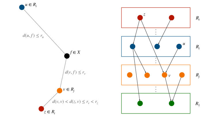
Figure 1: An example contact DAG. Arcs are constructed per Definition 5.

Our first observation is that the W$k$PP instance has a good fractional solution, and since the LP is integral, it also has a good integral solution. The proof of this claim, i.e. Lemma 6, is based on standard network flow ideas.

Lemma 6.

There is a valid solution to W$k$PP LP of value at least $m$ for the W$k$PP instance $\mathcal{J}$. Since W$k$PP LP is integral, this implies $\mathcal{J}$ has an integral solution of value at least $m$.

Proof.

We construct a fractional solution $y$ for the W$k$PP LP with objective value at least $m$. Recall $V=\bigcup_{i}R_{i}$ per definition of contact DAG. For any $f\in X$ let $A_{f}:=\{v\in V\mid d(f,v)\leq r_{v}\}$ be the set of points $v\in V$ for which $x_{f}$ contributes to $\textsf{cov}(v)$. That is for all $v\in V$:

$$\sum_{\begin{subarray}{c}f\in X:\\ v\in A_{f}\end{subarray}}x_{f}=\textsf{cov}(v).$$ (1)

There is an edge between points $u,v\in V$ iff there exists some $f\in X$ for which $d(u,f)\leq r_{u}$ and $d(v,f)\leq r_{v}$. Thus for any $u,v\in A_{f}$, we have $(u,v)\in E$. Now recall how we augmented $G$ to get a flow network $G^{\prime}$ by adding source and sink vertices $s$ and $t$, plus arcs $(s,v)$ and $(v,t)$ for all $v\in V$. Observe that $A_{f}$ resembles an $s,t$ path in $G^{\prime}$. Formally, let $(u_{1},\dots,u_{l})$ be $A_{f}$ sorted in decreasing order of neighborhood radii. Define $p_{f}$ to be the $s,t$ path that passes through $A_{f}$ in this order. That is, $p_{f}=((s,u_{1}),(u_{1},u_{2}),\dots(u_{l},t))$. Note that the same arc can be in $p_{f}$ of multiple $f\in X$. This motivates the definition of $H_{e}:=\{f\in X\mid e\in p_{f}\}$. Set $y$ as follows:

$$y_{e}:=\sum_{f\in H_{e}}x_{f}.$$

Now we argue that $y$ is a feasible solution for W$k$PP LP. First, notice that the flow is conserved for each vertex $v\in V$. That is, $\sum_{e\in{\delta^{-}}(v)}y_{e}=\sum_{e\in{\delta^{+}}(v)}y_{e}$. This is due to the fact that for any $f\in X$, we add the same amount $x_{f}$ to $y_{e}$ of all $e\in p_{f}$. Next, we see that $\textsf{flow}(v)=\textsf{cov}(v)$.

$$\textsf{flow}(v)=\sum_{e\in{\delta^{-}}(v)}y_{e}=\sum_{e\in{\delta^{-}}(v)}\sum_{f\in H_{e}}x_{f}=\sum_{\begin{subarray}{c}f\in X:\\ v\in A_{f}\end{subarray}}x_{f}=\textsf{cov}(v).$$ (2)

The constraint $\textsf{flow}(v)\leq 1$ and $\textsf{flow}(t)\leq k$ in W$k$PP LP follow from similar constraints in P$k$CO LP: The former is due to the constraint $\textsf{cov}(v)\leq 1$ and the latter is by $\sum_{f\in X}x_{f}\leq k$.

The last thing to verify is that the value of the W$k$PP LP objective for this solution is at least $m$. That is, is $\sum_{v\in V}\textsf{flow}(v)\lambda(v)\geq m$. We start with the constraint $m\leq\sum_{v\in X}\textsf{cov}_{v}$ from P$k$CO LP:

$$m\leq\sum_{v\in X}\textsf{cov}(v) =\sum_{u\in V}\sum_{v\in C(u)}\textsf{cov}(v)$$ (by 3)

$$\leq\sum_{u\in V}|D(u)|\textsf{cov}(u)$$ (by 1)

$$=\sum_{u\in V}|D(u)|\textsf{flow}(u)=\sum_{u\in V}\textsf{flow}(u)\lambda(u). \lambda$$ (By (2) and Definition of )

∎

Theorem 4 now follows from the following lemma.

Lemma 7.

Any solution with value at least $m$ for the W$k$PP instance $\mathcal{J}$ given by Algorithm 2 translates to a 9-approximation for the P$k$CO instance $\mathcal{I}$.

Before proving Lemma 7, we begin with a few observations. Per the definition of contact DAG we have the following property.

Fact 2.

If $u\in R_{i}$, $v\in R_{j}$, and $(u,v)$ is an arc in contact DAG, $d(u,v)\leq r_{u}+r_{v}$.

Note that the converse of 2 does not necessarily hold. The next fact follows straightforwardly from 1; by construction, $\{C_{i}\}_{i\in[t]}$ partitions $X$ and Filter further partitions each $C_{i}$ according to 1(b).

Fact 3.

$\{D(v),v\in V\}$ as constructed in Algorithm 2 partitions $X$.

In the following claim, we bound the distances between points on a contact DAG, and therefore are bounding the distances between points on any path that could be returned for the W$k$PP instance.

Claim 8.

For any $u\in R_{i}$, $v\in R_{j}$ reachable from $u$ in a contact DAG, $d(u,v)<3\cdot 2^{i}$.

Proof.

Observe that by definition of contact DAG, $i>j$. A path from $u$ to $v$ may contain a vertex from any level of the DAG between $i$ and $j$. In the worst case, the path has a vertex $w_{k}$ from every level $R_{k}$ for $j<k<i$:

$$d(u,v) \leq d(u,w_{i-1})+d(w_{i-1},w_{i-2})+\ldots+d(w_{j+1},v)$$

$$\leq(r_{u}+r_{w_{i-1}})+(r_{w_{i-1}}+r_{w_{i-2}})+\ldots+(r_{w_{j+1}}+r_{v})$$ (by 2)

$$=r_{u}+2\sum_{k=j+1}^{i-1}r_{w_{k}}+r_{v}<r_{u}+2\sum_{k=1}^{i-1}2^{k} w_{k}\in C_{k}$$ (by definition of )

$$=r_{u}+2\cdot(2^{i}-2)<3\cdot 2^{i}. r_{u}<2^{i}$$ ()

Note the slack which leads to the first strict inequality; indeed, we would still have this inequality if there was an extra $r_{v}$ in the summation. This slack is utilized when we move to more general versions of the problem, in particular, in 16 and in Appendix C. ∎

Now we are armed with all the facts needed to prove Lemma 7.

Proof of Lemma 7.

We are assuming the constructed W$k$PP instance has a solution of value at least $m$, which means there exists a set of $k$ disjoint paths $P\subseteq\mathcal{P}(G)$ in the contact DAG such that $\textsf{val}(P)\geq m$. For any path $p\in P$, let $\textsf{sink}(p)$ denote the last node in this path (i.e. $\textsf{sink}(p)=\arg\min_{u\in p}r_{u}$). Our final solution would be $S:=\{\textsf{sink}(p):p\in P\}$. We argue that this $S$ is a 9-approximate solution for the initial P$k$CO instance. Since $P$ has at most $k$ many paths, $|S|\leq k$.

Now we show any $w\in D(u)$ where $u\in p\in P$, can be covered by $v=\textsf{sink}(p)$ with dilation at most 9. Assume $u\in R_{i}$ for some $i\in[t]$.

$$d(w,v) \leq d(w,u)+d(u,v)<r_{w}+r_{u}+3\cdot 2^{i} \text{(by~{}\lx@cref{creftypecap~refnum}{fact:arcdist} and \lx@cref{creftypecap~refnum}{clm:dist2root}})$$

$$<r_{w}+4\cdot 2^{i}\leq 9r_{w}. r_{u}<2^{i} 2^{i-1}\leq r_{w}$$ ( and )

The last piece is to argue at least $m$ points will be covered by $S$. The set of points that are covered by $S$ within $9$ times their radius is precisely the set $D_{\textsf{total}}:=\bigcup_{p\in P}\bigcup_{u\in p}D(v)$. So we need to show $|D_{\textsf{total}}|\geq m$. By 3 we have:

$$|D_{\textsf{total}}|=|\bigcup_{p\in P}\bigcup_{v\in p}D(v)|=\sum_{p\in P}\sum_{v\in p}|D(v)|=\textsf{val}(P),$$

where the last equality is by the definition of $\lambda(v),v\in V$ (in Line 3 of Algorithm 2) and definition of $\textsf{val}(P)$. By assumption $\textsf{val}(P)\geq m$ thus $D_{\textsf{total}}$ contains at least $m$ points. ∎

As previously stated, Lemma 7 along with Lemma 6 together complete the proof of Theorem 4.

Remark 9.

In the special case where there are 2 types of radii, we can slightly modify our approach to get a 3-approximation algorithm. This result is tight. To see this consider P$k$CO instances where clients having priority radii of either $0$ or $1$, with $n_{0}$ of the former type and $n_{1}$ of the latter, and the number of outliers allowed is $n_{0}-k$. Clients with priority radii $0$ either need to have a facility opened at that same point, or need to be an outlier. Since only $n_{0}-k$ outliers and $k$ centers are allowed, all the outliers and centers are on these $n_{0}$ points. Thus, the $n_{0}$ points act as facilities in the $k$-Supplier problem which is hard to approximate with a factor better than 3. This shows a gap with the $k$-Center with outliers, which has a $2$-approximation [9].

In general, our framework yields improved approximation factors when the number of distinct radii is less than 5 (see Theorem 10). In the special case when all input radii are already powers of $2$ (foregoing the loss incurred from bucketing), our algorithm is actually a $5$-approximation. This factor improves if the radii are powers of some $b>2$ and approaches $3$ as $b$ goes to infinity (see Theorem 11).

Theorem 10.

There is a $(2t-1)$-approximation for P$k$CO instances where there are only $t\geq 2$ types of radii.

Proof.

Given P$k$CO instance $\mathcal{I}$ with $t\geq 2$ distinct types of radii, $r_{1}<r_{2}<\dots<r_{t}$, obtain a fractional solution $x$ by solving the P$k$CO LP. Partition $X$ according to each point’s radius into $C_{1},\dots,C_{t}$, where $C_{i}$ is points of radius $r_{i}$ for $i\in[t]$. Construct a W$k$PP instance $\mathcal{J}$ by running Algorithm 2 with input cov corresponding to $x$. Assuming the W$k$PP instance has a solution with value at least $m$, we can show how to obtain a $(2t-1)$-approximate solution as follows. Let $P$ be the W$k$PP solution. Take any $p\in P$. If $p$ is a single vertex, simply add it to solution $S$. Otherwise, let $v=\textsf{sink}(p)$ where $v\in R_{j}$ for some $j\in[t]$, and $v^{\prime}$ is the vertex before $v^{\prime}$ in $p$, i.e. $v^{\prime}\in p$ where $v^{\prime}\in R_{j^{\prime}}$ for some $j^{\prime}\in[t]$ such that $j^{\prime}>j$, and $p$ contains the directed edge $(v^{\prime},v)$. Now, instead of adding the point $v$ to $S$, as was done in the proof of Lemma 7, we instead add the point $f\in X$ that covers both $v$ and $v^{\prime}$ within distance $r_{j}$ and $r_{j^{\prime}}$, respectively. Such an $f$ exists per Definition 5.

For points $w\in D(v)$ and so $r(w)=r_{j}$, we have $d(w,f)\leq d(w,v)+d(v,f)\leq 2r_{j}+r_{j}=3r_{j}$, and thus $w$ is covered by $f$ with dilation at most $3\leq 2t-1$ since $t\geq 2$. The exact same argument holds if $w\in D(v^{\prime})$ and $r(w)=r_{j^{\prime}}$. For any $w\in D(u)$ where $u\in p$ and $u\in R_{i}$ for some $i\in[t]$ such that $i>j^{\prime}$, we can bound the distance between $u$ and $v^{\prime}$ similar to the proof of 8. However, since we do not bucket radii values by powers of $2$, we instead bound the radius of any vertex between $u$ and $v^{\prime}$ by $r_{i}$. Using this, and the fact that $j^{\prime}>j$ implies that $j^{\prime}\geq 2$, we can derive that

$$d(u,v^{\prime})\leq r_{i}+2\sum_{k=j^{\prime}+1}^{i-1}r_{k}+r_{j^{\prime}}<2\sum_{k=3}^{i}r_{i}=2(i-2)r_{i}.$$

Recall that $d(w,u)\leq 2r_{i}$ (1) and $d(v^{\prime},f)\leq r_{j^{\prime}}\leq r_{i}$. Using this and triangle inequality, we can conclude that

$$d(w,f)\leq d(w,u)+d(u,v^{\prime})+d(v^{\prime},f)<3r_{i}+2(i-2)r_{i}=(2i-1)r_{i}.$$

Thus, $w$ will be covered by $f$ with dilation at most $2i-1\leq 2t-1$.

To argue at least $m$ points will be covered by $S$, follow the analogous argument from the proof of Lemma 7. The remainder of this proof, i.e. showing that $\mathcal{J}$ does indeed have a solution of value at least $m$ that can be determined in polynomial time using an MCMF algorithm, is identical to the proof of Lemma 6. ∎

Theorem 11.

There is a $((3b-1)/(b-1))$-approximation for P$k$CO instances where the radii are powers of $b\geq 2$.

Proof.

Given P$k$CO instance $\mathcal{I}$ obtain fractional solution $x$ by solving the P$k$CO LP. Partition $X$ according to each point’s radius into $C_{1},\dots,C_{t}$, where $t:=\lceil\log_{b}r_{max}\rceil$ and $C_{i}:=\{v\in X\mid r_{v}=b^{i-1}\}$ for $i\in[t]$. Construct a W$k$PP instance $\mathcal{J}$ by running Algorithm 2 with input cov corresponding to $x$. Assume the W$k$PP instance has a solution $P$ with value at least $m$. For any $p\in P$ add $v=\textsf{sink}(p)$ to solution $S$. Consider arbitrary $w\in D(u)$ where $u\in p\in P$ and assume $u\in R_{i}$ for some $i\in[t]$. Similar to the proof of 8 one can show $d(u,v)<((b+1)/(b-1))\times b^{i-1}$. By 1 $d(w,u)\leq r_{w}+r_{u}=2b^{i-1}$. Thus any $w$ is covered by dilation $(3b-1)/(b-1)$ as $d(w,v)\leq d(w,u)+d(u,v)<2b^{i-1}+((b+1)/(b-1))\times b^{i-1}=(3b-1)/(b-1)r_{w}$.

As in the proof of Theorem 10, the remaining pieces of this proof will follow the analogous arguments from the proofs of Lemma 7 and Lemma 6. ∎

Before proceeding to the next sections, we make the following observation which will help us in handling more general constraints on the choice of facilities. The only place we used the cardinality constraint on the facilities (i.e. $\sum_{f\in X}x_{f}\leq k$) is to make sure that the solution $y$ corresponds to at most $k$ many paths. The reduction to the path problem and the analysis of the approximation ratio do not dependent on the specifics of the constraint.

4 Priority Matroid Center with Outliers

In this section, we generalize the results from the previous section to the Priority Matroid Center with Outliers problem.

Definition 6 (Priority Matroid Center with Outliers (PMCO)).

The input is a metric space $(X,d)$, parameter $m\in\mathbb{N}$, radius function $r:X\to\mathbb{R}_{>0}$, and $\mathscr{F}\subseteq 2^{X}$ a family of independent sets of a matroid. The goal is to find $S\in\mathscr{F}$ to minimize $\alpha$ such that for at least $m$ points $v\in X$, $d(v,S)\leq\alpha\cdot r(v)$.

Theorem 12.

There is a 9-approximation for PMCO.

As in the previous section, we assume $\alpha=1$ and consider the feasibility version of the problem. For any $S\subseteq X$, let $\textsf{rank}_{\mathscr{F}}(S)$ be the rank of $S$ in the given matroid. The natural LP relaxation for this problem is very similar to that of P$k$CO LP except that we replace the cardinality constraints with rank constraints $x(S)\leq\textsf{rank}_{\mathscr{F}}(S)$ for all $S\subseteq X$. This is because for any $S\in\mathscr{F}$, $|S|=\textsf{rank}_{\mathscr{F}}(S)$.

$$\sum_{v\in X}\textsf{cov}(v) \geq m$$ (PMCO LP)

$$\sum_{v\in S}x_{v} \leq\textsf{rank}_{\mathscr{F}}(S) \forall S\subseteq V$$

$$\textsf{cov}(v):=\sum_{\begin{subarray}{c}u\in X:\\ d(u,v)\leq r_{v}\end{subarray}}x_{u} \leq 1 \forall v\in X$$

$$0\leq x_{v} \leq 1 \forall v\in X.$$

Similar to W$k$PP, the path packing version of PMCO defined below. Recall from the previous section, that after reducing from P$k$CO to W$k$PP we returned a set of $k$ vertices in DAG $G$ as our final solution. Now that we have matroid constraints, we must instead return a set $S$ of vertices such that $S\in\mathscr{F}$. Doing so is not entirely straightforward, since our reduction does not guarantee that such a subset of vertices actually exists and covers enough points in their corresponding vertex disjoint paths. Instead, we show there is an $S\in\mathscr{F}$ such that each member of this $S$ is close to some vertex of $G$. These close points in $G$ will correspond to a set of vertex disjoint paths that will cover enough points.

Definition 7 (Weighted $\mathscr{F}$-Path Packing).

The input is a DAG $G=(V,E)$, $\lambda:V\rightarrow\mathbb{Z}_{+}$, a finite set $X$, a set $\mathcal{Y}=\{Y_{v}\subseteq X\mid v\in V\}$, and a down-closed family $\mathscr{F}\subseteq 2^{X}$ of independent sets. The goal is to find a set of vertex disjoint paths $P\subseteq\mathcal{P}(G)$ in $G$ with maximum $\textsf{val}(P):=\sum_{p\in P}\sum_{v\in p}\lambda(v)$ with the following constraint: there exists a set $S\in\mathscr{F}$ such that $\forall p\in P$, $S\cap Y_{\textsf{sink}(p)}\neq\emptyset$ where $\textsf{sink}(p)$ is the last vertex of the path $p$.

When $\mathscr{F}$ is the collecton of independent set of a matroid on $X$, we refer to the preceding problem as the Weighted Matroid Path Packing problem (WMatPP).

In the preceding definition, the collection of sets $\mathcal{Y}$ is meant to describe the set of points in $X$ that a vertex in $G$ can be considered close to. As mentioned previously, such a set is needed because the selected paths of $G$ need to correspond to a set from $\mathscr{F}$. Notice that per this definition, $\mathscr{F}$ has no requirement besides it being a family of independent sets of a matroid described on $X$, and $X$ could be separate from $G$ (though, for our reduction, we do ultimately construct $G$ with respect to our PMCO input point set $X$). It may be helpful to notice that WMatPP is a generalization of W$k$PP from the previous section (Definition 4): if $V\subseteq X$ and the matroid from which $\mathscr{F}$ is described is a uniform matroid, i.e. $\mathscr{F}$ contains all subsets $S\subseteq X$ such that $|S|\leq k$, then collection $\mathcal{Y}$ can simply be set to $\{\{v\}\mid v\in V\}$, resulting in an instance equivalent to W$k$PP.

Now, observe that the reduction procedure in Algorithm 2 and all of our subsequent observations in Section 3.1 do not rely on how we define a feasible set of centers. Hence, the main obstacle in proving Theorem 12 lies in our reduction to MCMF. Luckily, the result of [12] helps us address this by giving LP integrality results similar to MCMF using the following formulation on directed polymatroidal flows [18, 23, 30]: For a network $G^{\prime}=(V^{\prime},E^{\prime})$, for all $v\in V^{\prime}$, we are given polymatroids $\rho^{-}_{v}$ and $\rho^{+}_{v}$ on ${\delta^{-}}(v)$ and ${\delta^{+}}(v)$ respectively. For every arc $e\in E^{\prime}$ there is a variable $0\leq y_{e}\leq 1$. The capacity constraints for each $v\in V^{\prime}$ are defined as:

$$\sum_{e\in U}y_{e} \leq\rho^{-}_{v}(U)\qquad\forall U\subseteq{\delta^{-}}(v)$$

$$\sum_{e\in U}y_{e} \leq\rho^{+}_{v}(U)\qquad\forall U\subseteq{\delta^{+}}(v).$$

We augment the DAG $G$ given in WMatPP to construct a polymatroidal flow network $G^{\prime}$. In this new network, $V^{\prime}=V\cup X\cup\{s,t\}$ (see Remark 13) where each node $v\in V$ has cost $-\lambda(v)$. $E^{\prime}$ includes all of $E$, plus arcs $(s,v)$ for all $v\in V$. Finally, instead of adding arcs $(v,t)$, we add arcs $(v,f)$ and $(f,t)$ for all $f\in Y_{v}$.

Remark 13.

Even though a vertex $v\in V$ might correspond to a point in $X$, in $V^{\prime}$ we make a distinction between the two copies.

The polymatroids for this instance are constructed as follows: for any $v\in V\cup X$, $\rho^{-}_{v}(U)=1$ for all non-empty $U\subseteq{\delta^{-}}(v)$ and $\rho^{+}_{v}$ is defined similarly on ${\delta^{+}}(v)$. For $s$, we only have outgoing edges where $\rho^{+}_{s}(U)=|U|$ for all $U\subseteq{\delta^{+}}(s)$. Finally, we enforce the matroid constraints of $\mathscr{F}$ on $t$. For any $U\subseteq{\delta^{-}}(t)$, let $T\subseteq X$ be the set of starting nodes in $U$. That is, $U=\{(f,t):f\in T\}$. Set $\rho^{-}_{t}(U)=\textsf{rank}_{\mathscr{F}}(T)$. Since ${\delta^{-}}(t)\subseteq X$, these capacity constraints on $t$ are equivalent to the following set of constraints:

$$\sum_{f\in T}y_{(f,t)}\leq\textsf{rank}_{\mathscr{F}}(T)\qquad\forall T\subseteq X:\{(f,t):f\in T\}\subseteq{\delta^{-}}(t).$$

Now, we prove a claim analogous to that of 5.

Claim 14.

WMatPP is equivalent to solving the polymatroidal flow on network $G^{\prime}$.

Proof.

Any solution $P$ for the WMatPP instance translates to a valid flow of cost $-\textsf{val}(P)$ for the flow problem. Let $S\in\mathscr{F}$ be the independent set that intersects $Y_{\textsf{sink}(p)}$ for all $p\in P$. For any path $p\in P$ with start vertex $u$ and sink vertex $v$, take arbitrary $f\in S\cap Y_{v}$. Send one unit of flow from $s$ to $u$, through $p$ to $v$ and then to $f$ and $t$. All the polymatroidal constraints in WMatPP LP are satisfied.

Now we argue that any solution to the flow instance with cost $-m$ translates to a solution $P$ for WMatPP with $\textsf{val}(P)=m$. To see this, note that the flow solution consists of $s,t$ paths that are vertex disjoint with respect to $V\cup X$. This is due to our choice of $V\cup X$ polymatroids. Each path passes through one $v\in V$, then immediately to $f\in Y_{v}$ and then ends in $t$. By polymatroidal constraints on $t$, the subset of $X$ that has a flow going through it will be an independent set of $\mathscr{F}$.

Let $P$ be the described paths induced on $V$. For $v\in V$, $-\lambda(v)$ is counted towards the MCMF cost iff $v$ has flow passing through it. This means $v$ is included in some path in $P$. Thus $\textsf{val}(P)=m$. ∎

The polymatroidal LP for this particular construction is as follows (recall $\textsf{flow}(v):=\sum_{e\in{\delta^{-}}(v)}y_{e}$):

$$\max \sum_{v\in V}\textsf{flow}(v)\lambda(v)$$ (WMatPP LP)

$$\textsf{flow}(v) :=\sum_{e\in{\delta^{-}}(v)}y_{e}=\sum_{e\in{\delta^{+}}(v)}y_{e} \forall v\in V\cup X$$

$$\sum_{f\in T}y_{(f,t)} \leq\textsf{rank}_{\mathscr{F}}(T) \forall T\subseteq X:\{(f,t):f\in T\}\subseteq{\delta^{-}}(t)$$

$$\textsf{flow}(v) \leq 1 \forall v\in V\cup X$$

$$0\leq y_{e} \leq 1 \forall e\in E^{\prime}$$

By [12], WMatPP LP is integral and there are polynomial time algorithms to solve it.

For our reduction from PMCO to WMatPP, most of the notation and results can be recycled from Section 3.1. Specially, the reduction itself (Algorithm 3) is just Algorithm 2 along with the explicit construction of the sets of $\mathcal{Y}$ (5).

Remark 15.

Per the definition of arc in contact DAG, as well as our setting of $Y_{v}$ given in 5 of Algorithm 3, for two nodes $u,v\in V$, $(u,v)$ is an arc iff $Y_{v}$ intersects $Y_{u}$.

Algorithm 3 Reduction to WMatPP

1:PMCO instance $\mathcal{I}=$$((X,d),r,\mathscr{F},m)$ and assignment $\{\textsf{cov}(v)\in\mathbb{R}_{\geq 0}:v\in X\}$

2:$R_{i},\{D(u):u\in R_{i}\}\leftarrow\textsf{Filter}((C_{i},d),r,\textsf{cov})$ for all $i\in[t]$

3:Construct contact DAG $G=(V,E)$ per Definition 5

4:$\lambda(v)\leftarrow|D(v)|$ for all $v\in V$

5:$Y_{v}\leftarrow\{u\in X:d(u,v)\leq r_{v}\}$ for all $v\in V$

6:WMatPP instance $(G=(V,E),\lambda,X,\mathcal{Y}=\{Y_{v}\mid v\in V\},\mathscr{F})$

Before we begin proving our 9-approximation result for PMCO, we need to slightly modify 8 to account for the fact that a vertex covered by $v$ (the sink of some path) has to travel slightly farther than $v$ to reach an $f\in Y_{v}$. Fortunately, the proof of 8 has a slight slack that allows us to derive the same distance guarantees even with this extra step.

Claim 16.

For any $u\in R_{i}$ and $v\in R_{j}$ reachable from $u$ in contact DAG $G$, and any $f\in Y_{v}$, $d(u,f)<3\cdot 2^{i}$.

Proof.

By definition of $G$ it must be the case that $i>j$. Also for all $f\in Y_{v}$, $d(f,v)\leq r_{v}$. If $v$ is reachable from $u$, a path between $u$ and $v$ may contain a vertex $w_{k}$ from every level $R_{k}$ for $j<k<i$:

$$d(u,f) \leq d(u,v)+d(v,f)\leq d(u,v)+r_{v}$$

$$\leq(r_{u}+r_{w_{i-1}})+(r_{w_{i-1}}+r_{w_{i-2}})+\ldots+(r_{w_{j+1}}+r_{v})+r_{v}$$ (by 2)

$$\leq r_{u}+2\sum_{k=1}^{i-1}2^{k} C_{k}$$ (by definition of )

$$=r_{u}+2\cdot(2^{i}-2)<3\cdot 2^{i}. u\in C_{i} r_{u}<2^{i}$$ (, )

∎

Since the previous claim has the same guarantee as 8, Lemma 7 easily translates to the following:

Lemma 17.

Any solution with value at least $m$ for the output of Algorithm 3 translates to a 9-approximation for the input $\mathcal{I}$.

Proof.

Let $P\subseteq\mathcal{P}(G)$ be the promised WMatPP solution. Let $S\in\mathscr{F}$ be the independent set that intersects $Y_{\textsf{sink}(p)}$ for all $p\in P$. By 16, $S$ covers all the vertices $v\in V$ that are included in $P$ by dilation 3. Proof of Lemma 7 shows that for any such $v\in V$ covered by $P$ and any $w\in D(v)$, $d(w,S)\leq 9r_{w}$. This holds for at least $m$ points. ∎

We can now prove our 9-approximation result for PMCO.

Proof of Theorem 12.

The algorithm is very similar to that of Theorem 4: Given PMCO instance $\mathcal{I}=$$((X,d),r,\mathscr{F},m)$, solve the PMCO LP and use the solution in the procedure of Algorithm 3 to reduce to WMatPP instance $\mathcal{J}=\text{$(G=(V,E),\lambda,X,\mathcal{Y},\mathscr{F})$}$. Let $P\subseteq\mathcal{P}(G)$ be the solution to this instance and $S\in\mathscr{F}$ be the independent set that intersects $Y_{\textsf{sink}(p)}$ for all $p\in P$. If $\textsf{val}(P)\geq m$, $S$ is a 9-approximate solution for $\mathcal{I}$ via Lemma 17. So we prove such solution $P$ exists by constructing a feasible (possibly fractional) WMatPP LP solution.

Take the contact DAG from Algorithm 3, $G=(V,E)$, and recall that each $v\in V$ is also a point in $X$. For any $f\in X$ let $A_{f}:=\{v\in V:d(f,v)\leq r_{v}\}$ be the set of points $v\in V$ for which $x_{f}$ contributes to $\textsf{cov}(v)$. By definition of an edge in contact DAG, for any $u,v\in A_{f}$, we have $(u,v)\in E$. Define $p_{f}$ to be the $s,t$ path that passes through $A_{f}$ in the order of decreasing neighborhood radii. Formally, let $(u_{1},\dots,u_{l})$ be $A_{f}$ sorted in decreasing order of neighborhood radii. Then, $p_{f}=((s,u_{1}),(u_{1},u_{2}),\dots(u_{l},f),(f,t))$. Similar to the proof of Theorem 4 we define $H_{e}:=\{f\in X:e\in p_{f}\}$ and set $y$ as follows:

$$y_{e}:=\sum_{f\in H_{e}}x_{f}.$$

Now, we argue that $y$ is a feasible solution for WMatPP LP with objective value at least $m$. The flow is conserved for each vertex $v\in V\cup X$ since for any $f\in X$, we add the same amount $x_{f}$ to $y_{e}$ of all $e\in p_{f}$. Observe that $\textsf{flow}(v)=\textsf{cov}(v)$ thus the constraint $\textsf{cov}(v)\leq 1$ in P$k$CO LP implies $\textsf{flow}(v)\leq 1$. To see why the rank constraints are satisfied, the key observation is that any $e\in{\delta^{-}}(t)$ must be of the form $(f,t)$ for some $f\in X$, and by our construction $y_{e}=x_{f}$. So according to constraint $\sum_{f\in T}x_{f}\leq\textsf{rank}_{\mathscr{F}}(T)$ in PMCO LP we have $\sum_{f\in T}y_{(f,t)}\leq\textsf{rank}_{\mathscr{F}}(T)$. Lastly, one can follow the argument from the proof of Theorem 4 to show that the WMatPP LP objective for this solution will be at least $m$. ∎

5 Priority Knapsack Center with Outliers

In this section, we discuss the Priority Knapsack Center with Outliers (PKnapCO) problem.

Definition 8 (Priority Knapsack Center with Outliers (PKnapCO)).

The input is a metric space $(X,d)$, a radius function $r:X\to\mathbb{R}_{>0}$, a weight function $\textsf{w}:X\to\mathbb{R}_{\geq 0}$, parameters $B>0$ and $m\in\mathbb{N}$. The goal is to find $S\subseteq X$ with $\textsf{w}(S)\leq B$ to minimize $\alpha$ such that for at least $m$ points $v\in X$, $d(v,S)\leq\alpha\cdot r(v)$.

Theorem 18.

There is a 14-approximation for PKnapCO.

As in the previous sections, we assume $\alpha=1$ and work with the feasibility version of the problem. We reduce PKnapCO to the following path packing problem. Notice that this definition is nearly the same as that of WMatPP in that we need a specified $\mathcal{Y}$ to describe points close to each vertex of the input DAG. In place of the matroid constraint, here we have a knapsack constraint.

Definition 9 (Weighted Knapsack Path Packing (WNapPP)).

The input is DAG $G=(V,E)$, $\lambda$, finite set $X$, and $\mathcal{Y}=\{Y_{v}\subseteq X:v\in V\}$ (as in WMatPP), as well as weight function $\textsf{w}:X\rightarrow\mathbb{R}_{\geq 0}$ and parameter $B>0$. The goal is to find a set of disjoint paths $P\subseteq\mathcal{P}(G)$ with maximum $\textsf{val}(P)$ for which there exists $S\subseteq X$ with $w(S)\leq B$ such that $\forall p\in P$, $S\cap Y_{\textsf{sink}(p)}\neq\emptyset$.

There are two main issues in generalizing our techniques from Section 3 and Section 4 to handle the knapsack constraint. First, the WNapPP problem seems hard on a general DAG. To circumvent this, we make two changes to the LP-aware PKnapCO to WNapPP reduction. First, we modify Algorithm 1 so that a representative captures points at larger distances. To be precise, for a representative $u$, 7 is modified to: $D(u)\leftarrow\{v\in U:d(u,v)\leq r_{u}+2r_{v}\}$. Second, the partition induced by $C_{i}$’s in Algorithm 2 is done via powers of $4$ instead of $2$. This is what bumps our approximation factor from 9 to 14. However, this dilation allows the resulting contact DAG to be a directed out-forest. It is not too hard to solve WNapPP when $G$ is a directed-out forest using dynamic programming (details of this DP algorithm can be found in Appendix A).

The second issue, however, is more serious: After reducing to WNapPP we cannot guarantee that the path packing problem has a good integral solution using cov from the natural PKnapCO LP solution. This is because the natural LP relaxation for PKnapCO has an unbounded integrality gap (even in the single radius case) [13].

We circumvent this by using the round-or-cut framework of [15]. Instead of using the PKnapCO LP, we would use cov in the convex hull of the integral solutions (call it $\mathscr{P}_{\textsf{cov}}$). Of course, we do not know the integral solutions and there may indeed be exponentially such solutions. So, we have to employ the ellipsoid algorithm. In each iteration of ellipsoid, we get some cov that may or may not be in $\mathscr{P}_{\textsf{cov}}$. In any case, if we manage to get a good path packing solution using this cov, we get an approximate PKnapCO solution and we are done. Otherwise, we are able to give ellipsoid a linear constraint that should be satisfied by any point in $\mathscr{P}_{\textsf{cov}}$ but is violated by the current cov. Ultimately, either we find an approximate solution for PKnapCO along the way, or ellipsoid prompts that $\mathscr{P}_{\textsf{cov}}$ is empty, indicating that the problem is infeasible.

From here on, let $\mathscr{F}$ be the set of all possible centers that fit in the budget. That is, $\mathscr{F}:=\{S\subseteq X:\textsf{w}(S)\leq B\}$. The following is the convex hull of the integral solutions for PKnapCO.

$$\textsf{$\mathscr{P}_{\textsf{cov}}$}=\{(\textsf{cov}(v):v\in X): \sum_{v\in X}\textsf{cov}(v) \geq ~{}~{}m \mathscr{P}_{\textsf{cov}}$$ (.1)

$$\forall v\in X, ~{}~{}\textsf{cov}(v) := \sum_{\begin{subarray}{c}S\in\mathscr{F}:\\ d(v,S)\leq r_{v}\end{subarray}}z_{S} \mathscr{P}_{\textsf{cov}}$$ (.2)

$$\sum\limits_{S\in\mathscr{F}}z_{S} = ~{}~{}1 \mathscr{P}_{\textsf{cov}}$$ (.3)

$$\forall S\in\mathscr{F}, z_{S} \geq 0\} \mathscr{P}_{\textsf{cov}}$$ (.4)

Observe that while the polytope has exponentially many auxiliary variables ($z_{S}$), its dimension is still $|X|$. In the next section, we will describe the whole reduction process.

5.1 Reduction to WNapPP

In this section, we describe how to reduce PKnapCO to WNapPP in detail since all the observations from Section 3.1 have to be modified to work on a forest instead of contact DAG.

From here on, we group clients by their neighborhood radius based on powers of 4, rather than 2. Partition $X$ according to each client’s neighborhood size into $C_{1},\dots,C_{t}$, where $C_{i}:=\{v\in X:4^{i-1}\leq r_{v}<4^{i}\}$ for $i\in[t]$. Let ModFilter be the modified Filter algorithm where the construction of $D(u)$ for a representative $u$ (7) is modified to:

$$D(u)\leftarrow\{v\in U:d(u,v)\leq r_{u}+2r_{v}\}.$$

As a result, two statements in  1 change to the following (recall $\phi$ is the input ordering which we usually initiate to cov):

Fact 4.

The following are true for the output of ModFilter: (a) $\forall u,v\in S,\phi(u)\geq\phi(v):\ d(u,v)>r_{u}+2r_{v}$, and (b)$\forall{u\in S},\forall{v\in D(u)}:\ d(u,v)\leq r_{u}+2r_{v}.$

Algorithm 4 shows the PKnapCO to WNapPP reduction. The algorithm constructs a directed forest called contact forest (see Definition 10) as a part of the WNapPP instance definition. We first run ModFilter on each $C_{i}$ to produce the vertices of our contact forest.

Algorithm 4 Reduction to WNapPP

1:PKnapCO instance $\mathcal{I}=$$((X,d),r,\textsf{w},B,m)$ and assignment $\{\textsf{cov}(v)\in\mathbb{R}_{\geq 0}:v\in X\}$

2:$R_{i},\{D(u):u\in R_{i}\}\leftarrow\textsf{ModFilter}((C_{i},d),r,\textsf{cov})$ for all $i\in[t]$

3:Construct contact forest $G=(V,E)$ per Definition 10

4:$\lambda(v)\leftarrow|D(v)|$ for all $v\in V$

5:$Y_{v}\leftarrow\{u\in X:d(u,v)\leq r_{v}\}$ for all $v\in V$

6:WNapPP instance $(G=(V,E),\lambda,X,\mathcal{Y}=\{Y_{v}\mid v\in V\},\textsf{w},B)$

Definition 10 (contact forest).

Let $R_{i}\subseteq C_{i}$, $i\in[t]$ be the set of representatives acquired after running ModFilter procedure on $C_{i}$ according to 2 of Algorithm 4. contact forest $G=(V,E)$ is a directed forest on vertex set $V=\bigcup_{i}R_{i}$ where the arcs are constructed by the as follows: For $u\in R_{i}$ and $v\in R_{j}$ where $i>j$, add the arc $(u,v)\in E$ if there exists $f\in X$ such that $d(u,f)\leq r_{u}$ and $d(v,f)\leq 2r_{v}$. Next, remove all the forward edges.

2 for contact DAG translates to the following fact for contact forest

Fact 5.

If $u\in R_{i}$, $v\in R_{j}$, and $(u,v)$ is an arc in contact forest, $d(u,v)\leq r_{u}+2r_{v}$.

A sharp reader may notice that we defined the contact forest to be a DAG in Definition 10 but referred to it as a forest of directed rooted trees elsewhere. Indeed one can show that the contact forest cannot have any cross edges so one can ignore the directions on the edges. We show this in the following claim.

Claim 19.

For $u\in R_{i}$ and $v\in R_{j}$, there is no $w\in R_{k}$ such that both $(u,w)$ and $(v,w)\in E$.

Proof.

Assume for the sake of contradiction that such a $u,v,w$ exists, hence $k<j$ and $k<i$. If $(u,w)$ and $(v,w)$ are both in $E$, then $d(u,w)\leq r_{u}+2r_{w}$ and $d(v,w)\leq r_{v}+2r_{w}$. By triangle inequality, we know that:

$$d(u,v)\leq r_{u}+r_{v}+4r_{w}<r_{u}+r_{v}+4^{k+1},$$

which is less than or equal to both $r_{u}+2r_{v}$ and $r_{v}+2r_{u}$ as $k<i$ and $k<j$. This means that either $(u,v)$ or $(v,u)$ must also be in $E$ which makes $(u,w)$ or $(v,w)$ a forward edge. However, since we have removed all forward edges from $G$, we reach a contradiction. ∎

The following lemma is what gives the approximation factor stated in Theorem 18.

Lemma 20.

Any solution with value at least $m$ for the output of Algorithm 4 translates to a $14$-approximation for the input $\mathcal{I}$.

Before proving the lemma, we will make the following observation on Algorithm 4.

Claim 21.

For any $u\in R_{i}$ and $v\in R_{j}$ reachable from $u$ in contact forest $G$ and any $f\in Y_{v}$, $d(u,f)<2\cdot 4^{i}$.

Proof.

By definition of $G$, it must be the case that $j<i$. Also for all $f\in Y_{v}$, $d(f,v)\leq r_{v}$. If $v$ is reachable from $u$, a path between $u$ and $v$ may contain a vertex $w_{k}$ from every level $R_{k}$ for $j<k<i$:

$$d(u,f) \leq d(u,v)+d(v,f)\leq d(u,v)+r_{v}$$

$$\leq(r_{u}+2r_{w_{i-1}})+(r_{w_{i-1}}+2r_{w_{i-2}})+\ldots+(r_{w_{j+1}}+2r_{v})+r_{v}$$ (by 5)

$$\leq r_{u}+3\sum_{k=1}^{i-1}4^{k} C_{k}$$ (by definition of )

$$=r_{u}+3\cdot((4^{i}-1)/3-1)<2\cdot 4^{i}. u\in C_{i} r_{u}<4^{i}$$ (since , )

∎

We are now armed with all the facts needed to prove Lemma 20.

Proof of Lemma 20.

Let $P\subseteq\mathcal{P}(G)$ be the promised WNapPP solution. Let $S\in\mathscr{F}$ be the set that intersects $Y_{\textsf{sink}(p)}$ for all $p\in P$. We will show that this $S$ is a $14$-approximate solution for the initial PKnapCO instance $\mathcal{I}$. For any $p\in P$ with sink node $v=\textsf{sink}(p)$ and any $u\in p$, $w\in D(u)$ is covered by dilation at most 14 through $f\in S\cap Y_{v}$. Assume $u\in R_{i}$ for some $i\in[t]$.

$$d(w,f) \leq d(w,u)+d(u,f)$$

$$<2r_{w}+r_{u}+2\cdot 4^{i}$$ (by 4 and 21)

$$<2r_{w}+3\cdot 4^{i} u\in C_{i} r_{u}<4^{i}$$ ( so )

$$\leq 14r_{w}. w\in C_{i} 4^{i-1}\leq r_{w}$$ ( so )

What remains is to show that $m$ points will be covered by $S$. The proof is identical to that in the proof of Lemma 7. ∎

In the next section, we show how to separate cov from $\mathscr{P}_{\textsf{cov}}$ if it is not valuable. That is, if after solving the output of Algorithm 4 the output WNapPP does not have a solution with value at least $m$, we can prove that the input cov is not in $\mathscr{P}_{\textsf{cov}}$.

5.2 The Round or Cut Approach

Given PKnapCO instance $\mathcal{I}$ and $\{cov(v):v\in X\}$, let $\mathcal{J}$ be the WNapPP instance output by Algorithm 4 on this input. We say cov is valuable if $\mathcal{J}$ has a solution with value at least $m$. In this section, we will show how to prove $\textsf{cov}\notin\textsf{$\mathscr{P}_{\textsf{cov}}$}$ if cov is not valuable.

The following lemma from [15] gives a valid set of inequalities that any point in $\mathscr{P}_{\textsf{cov}}$ has to satisfy.

Lemma 22 (from [15]).

Let $\lambda(v)\in\mathbb{R}$ for every $v\in X$ be such that

$$\sum_{\begin{subarray}{c}v\in X:\\ d(v,S)\leq r_{v}\end{subarray}}\lambda(v)<m\hskip 28.45274pt\forall S\in\mathscr{F},$$ (3)

Then any $\textsf{cov}\in\textsf{$\mathscr{P}_{\textsf{cov}}$}$ satisfies

$$\sum_{v\in X}\lambda(v)\textsf{cov}(v)<m.$$ (4)

Lemma 23.

If a given cov is not valuable, there is a hyperplane that separates it from $\mathscr{P}_{\textsf{cov}}$.

To prove this lemma, we need to first prove 24 and 25.

Claim 24.

If $\sum_{v\in X}\textsf{cov}(v)\geq m$ then $\lambda$ as defined in Algorithm 4 satisfies

$$\sum_{v\in X}\lambda(v)\textsf{cov}(v)\geq m.$$

Proof.

$$\sum_{v\in X}\lambda(v)\textsf{cov}(v) =\sum_{i}\sum_{v\in R_{i}}|D(v)|\textsf{cov}(v) \lambda$$ (by definition of )

$$\geq\sum_{i}\sum_{v\in R_{i}}\sum_{u\in D(v)}\textsf{cov}(u)$$ (by 1)

$$=\sum_{u\in X}\textsf{cov}(u).$$ (by 3)

∎

Claim 25.

For any solution $S\in\mathscr{F}$, there is a solution $P$ for the output of Algorithm 4 such that

$$\textsf{val}(P)=\sum\limits_{\begin{subarray}{c}v\in X:\\ d(v,S)\leq r_{v}\end{subarray}}\lambda(v).$$

Proof.

Observe that since $\lambda$ is only non-zero for representative points:

$$\sum\limits_{\begin{subarray}{c}v\in X:\\ d(v,S)\leq r_{v}\end{subarray}}\lambda(v)=\sum\limits_{\begin{subarray}{c}v\in V:\\ d(v,S)\leq r_{v}\end{subarray}}\lambda(v).$$

For any $f\in S$, let $A_{f}:=\{v\in V:d(v,f)\leq r_{v}\}$. Assume $A_{f}$’s are disjoint by assigning each covered point to an arbitrary facility in $S$ that covers it. So, we have that

$$\sum\limits_{\begin{subarray}{c}v\in V:\\ d(v,S)\leq r_{v}\end{subarray}}\lambda(v)=\sum_{f\in S}\sum_{v\in A_{f}}\lambda(v).$$

Fix some $f\in S$, and sort the members of $A_{f}$ according to the topological order in the contact forest. Let $u\in R_{i}$ and $v\in R_{j}$ be two consecutive members of $A_{f}$ in this order. Observe that the contact forest must contain an edge from $u$ to $v$ since $d(u,v)\leq d(u,f)+d(f,v)\leq r_{u}+r_{v}$. Hence $A_{f}$ corresponds to a path in contact forest (call it $p_{f}$). Since $A_{f}$’s are disjoint $p_{f}$’s are also vertex disjoint. Also every path sink is covered by $S$. That is, for any $p_{f}$ and $v=\textsf{sink}(p_{f})$ there is a member of $S$ (that is $f$) at distance at most $r_{v}$ from $v$. So the set $P=\{A_{f}\mid f\in S\}$ satisfies all the requirements of a feasible WNapPP solution. Furthermore,

$$\textsf{val}(P)=\sum_{p\in P}\sum_{v\in p}\lambda(v)=\sum_{f\in S}\sum_{v\in A_{f}}\lambda(v).$$

∎

Now the proof of Lemma 23 follows easily.

Proof of Lemma 23.

Through 25 we established the fact that for any $S\in\mathscr{F}$, there exists a WNapPP solution $P$ such that:

$$\textsf{val}(P)=\sum\limits_{\begin{subarray}{c}v\in X:\\ d(v,S)\leq r_{v}\end{subarray}}\lambda(v).$$

But by the assumption that cov is not valuable $\textsf{val}(P)<m$ hence:

$$\sum\limits_{\begin{subarray}{c}v\in X:\\ d(v,S)\leq r_{v}\end{subarray}}\lambda(v)<m.$$

This contradicts Lemma 22 since $\sum_{v\in X}\lambda(v)\textsf{cov}(v)<m$ is violated per 24 and can be used as a separating hyperplane. (Note, we can assume $\sum_{v\in X}\textsf{cov}(v)\geq m$ since if not, this itself can be used to separate cov). ∎

With this we complete the description of our round-or-cut approach.

Proof of Theorem 18.

Given PKnapCO instance $\mathcal{I}$, we can produce either a $14$-approximate solution or prove that it is infeasible. We start an ellipsoid algorithm on $\mathscr{P}_{\textsf{cov}}$. Given cov from ellipsoid, we feed $\mathcal{I}$ and cov to Algorithm 4 to get a WNapPP instance $\mathcal{J}$. Now we use the dynamic program in Appendix A to solve it. If the solution has value at least $m$, by Lemma 20 we have a $14$-approximate solution for $\mathcal{I}$ and are done. If not, we say cov is not valuable. Then, Lemma 23 gives us a separating hyperplane from the ellipsoid as proof that $\textsf{cov}\notin\textsf{$\mathscr{P}_{\textsf{cov}}$}$. After polynomially many iterations of ellipsoid, either we get an approximate solution for $\mathcal{I}$, or ellipsoid prompts that $\mathscr{P}_{\textsf{cov}}$ is empty and $\mathcal{I}$ is infeasible. ∎

6 Connections to Fair Clustering

In this section, we show how our results imply results in the two fairness notions as defined by [28] and [24].

6.1 “A Center in your Neighborhood” notion of [28]

Jung et al. [28] argue that fairness in clustering should take into account population densities and geography. For every $v\in X$, they define a neighborhood radius $\text{NR}(v)$ to be the distance to its $(\lceil n/k\rceil-1)$th nearest neighbor. They argue that a solution is fair if every $v$ is served within their $\text{NR}(v)$. They also observe that this may not always be possible, and therefore they wish to find a placement of centers $S\subseteq X$ minimizing $\max_{v}\frac{d(v,S)}{\text{NR}(v)}$. As an optimization problem, their problem is precisely an instantiation of Priority $k$-Center. Thus, one can easily obtain a $2$-approximation when we set $r(v)=\text{NR}(v)$.

[28] in fact show that it is always possible to find $S$ such that $d(v,S)\leq 2\text{NR}(v)$. They do so by looking at the centers obtained from running their algorithm (which is the same as that of Plesník). Note that a $2$-approximation to the instance of Priority $k$-Center defined by $r(v)=\text{NR}(v)$ does not necessarily imply this additional property. Here, we show why their finding is not a coincidence by considering the natural LP relaxation for Priority $k$-Center. Given an instance of Priority $k$-Center one can obtain a lower bound on the optimum value by finding the smallest $\alpha$ such that the following LP is feasible.

$$\mathrm{PkCFeasLP}(\alpha)~{}:=~{}\{(y_{u}\geq 0~{}:~{}u\in X):~{}~{}~{}\sum_{u\in X}y_{u}\leq k;~{}~{}~{}~{}\forall v\in X:\sum_{u:d(u,v)\leq\alpha r(v)}y_{u}\geq 1\}$$ (5)

Claim 26.

Suppose $\mathrm{PkCFeasLP}(\alpha)$ has a feasible solution, then Algorithm 1 run with $\phi(v)=\frac{1}{r(v)}$ finds at most $k$ centers that cover each point $v$ within distance $2\alpha r(v)$.

Proof.

The proof is similar to that of Theorem 2. Without loss of generality we can assume $\alpha=1$, otherwise we can scale all the radii by $1/\alpha$. We need to argue $|S|\leq k$. For any $u\in S$, we have $\sum_{v\in D(u)}y_{v}\geq 1$ since $B(u,r(u))\subseteq D(u)$. Since $D(u)$’s are disjoint and $\sum_{u\in X}y_{u}\leq k$, the claim follows. ∎

The preceding discussion and the claim shows the utility of viewing the clustering problem of [28] as a special case of Priority $k$-Center. One can then bring to bear all the positive algorithmic results on Priority $k$-Center (such as Theorem 3) to fine-tune the fair clustering model. Below we list a few other ways in which the Priority $k$-Center view could be useful.

• The LP relaxation could be useful in obtaining better empirical solutions. For example, it has been shown that for $k$-Center, the LP relaxation is integral under notions of stability [8].

• The model of [28] allows $\text{NR}(v)$ to be very large for points $v$ which may not be near many points. However, one may want to place an upper bound $M$ on the radius that is independent of $\text{NR}(v)$. The same algorithm yields a $2$-approximation but one may no longer have the property that all points are covered within twice $\text{NR}(v)$.

• In many scenarios, it makes sense to work with the Supplier version since it might not be possible to place centers at all locations in $X$. Second, there could be several additional constraints on the set of centers that can be chosen. Theorem 3 shows that more general constraints than cardinality can be handled.

• As previously mentioned, far away points in less dense regions (outliers) can be harmed by setting $\text{NR}(v)$ to be a large number. Alternatively, one can skew the choice of centers if one tries to set a small radius for these points. In this situation it is useful to have algorithms that can handle outliers such that one can find a good solution for vast majority of points and help the outliers via other techniques.

6.2 The Lottery Model of Harris et al. [24]

Harris et al. [24] define a lottery model of fairness where every client $v\in X$ has a “distance demand” $r(v)$ and a “probability demand” $\textsf{prob}(v)$. They deem a lottery, or distribution, over feasible solutions fair if every client is connected to a facility within distance $r(v)$ with probability at least $\textsf{prob}(v)$. The computational question is to figure out if this is (approximately) feasible. We show a connection to the outlier version of the Priority $k$-Center problem, and then generalize their results. To start, consider the following problem definition.

Definition 11 (Lottery Priority $\mathscr{F}$-Center (LP$\mathscr{F}$C)).

The input is a metric space $(X,d)$ where each point $v$ has a distance demand $r(v)>0$ and probability demand $\textsf{prob}(v)$. The input also (implicitly) specifies a family $\mathscr{F}\subseteq 2^{X}$ of allowed locations where centers can be opened. A distribution over $\mathscr{F}$ is $\alpha$-approximate if

$$\forall v\in X:~{}~{}~{}\Pr_{S\sim\mathscr{F}}[d(v,S)\leq\alpha\cdot r(v)]\geq\textsf{prob}(v).$$

An $\alpha$-approximation algorithm in the lottery model either asserts the instance infeasible in that a $1$-approximate distribution doesn’t exist, or returns an $\alpha$-approximate distribution.

Harris et al. [24] show that for the case when $\mathscr{F}$ is $\{S:|S|\leq k\}$, there is a $9$-approximate distribution. Using our aforementioned results, and a standard framework based on the Ellipsoid method (as in [17, 1]), we get the following results.

Theorem 27.

There is a 9-approximation for LP$\mathscr{F}$C where $\mathscr{F}$ is the independent set of a matroid.

Theorem 28.

There is a 14-approximation for LP$\mathscr{F}$C on points $X$ where $\mathscr{F}=\{S\subseteq X:\textsf{w}(S)\leq B\}$ for a poly-bounded weight function $\textsf{w}:X\to\mathbb{R}_{\geq 0}$ and parameter $B>0$.

We first describe the reduction. For this, we need to define the Fractional Priority $\mathscr{F}$-Center problem, in which each point comes with a (possibly fractional) weight $\mu_{v}$, and given $m\geq 0$, the goal is to find a set $S\in\mathscr{F}$ that covers a total weight of more than $m$ with minimum dilation of neighborhood radii.

Definition 12 (Fractional Priority $\mathscr{F}$-Center (FP$\mathscr{F}$C)).

The input is a metric space $(X,d)$ where each point $v$ has a radius $r_{v}>0$ and a weight $\mu_{v}\geq 0$. Given parameter $m\geq 0$ and a family of subsets of points $\mathscr{F}\subseteq 2^{X}$, the goal is to find $S\in\mathscr{F}$ to minimize $\alpha$ such that $\mu(\{v\in X$: $d(v,S)\leq\alpha\cdot r_{v}\})>m$.

An instance of FP$\mathscr{F}$C is specified by the tuple $((X,d),r,\mu,\mathscr{F},m)$. The following theorem states the reduction from LP$\mathscr{F}$C to FP$\mathscr{F}$C using the Ellipsoid method. The proof of this theorem can be found in Appendix B.

Theorem 29.

Given LP$\mathscr{F}$C instance $\mathcal{I}$ and a black-box $\alpha$-approximate algorithm $\mathcal{A}$ for FP$\mathscr{F}$C that runs in time $T(\mathcal{A})$, one can get an $\alpha$-approximate solution for $\mathcal{I}$ in time $\text{poly}(|\mathcal{I}|)T(\mathcal{A})$.

Now we discuss how our results generalize to solve FP$\mathscr{F}$C for matroid and knapsack constraints.

Proof of Theorem 27.

According to Theorem 29 we only need to prove that we can find a 9-approximate solution for any given FP$\mathscr{F}$C instance $\mathcal{I}=\text{$((X,d),r,\mu,\mathscr{F},m)$}$. First, observe that the LP for $\mathcal{I}$ is the same as PMCO LP with a minor modification: The constraint $\sum_{v\in X}\textsf{cov}(v)\geq m$ is changed to $\sum_{v\in X}\mu_{v}\textsf{cov}(v)>m$. Solve the LP for $\mathcal{I}$ and use the obtained cov to run the reduction in Algorithm 3 but with a change in 4: instead of setting $\lambda(v)\leftarrow|D(v)|$ for all $v\in V$, we will have $\lambda(v)\leftarrow\mu(D(v))$. This results in a WMatPP instance $\mathcal{J}$ with fractional $\lambda$. The procedure in [12] can handle fractional $\lambda$’s so we can still compute the solution for $\mathcal{J}$ in polynomial time. If this solution has value less than or equal to $m$, we know that $\mathcal{I}$ is infeasible. Otherwise, Lemma 17 tells us that this solution for $\mathcal{J}$ translates to a $9$-approximation for $\mathcal{I}$ and we are done. ∎

Proof of Theorem 28.

We follow a procedure similar to the proof of Theorem 27. Per Theorem 29 we only need to prove there is a 14-approximation for the FP$\mathscr{F}$C instance where $\mathscr{F}$ is a set of feasible knapsack solutions with poly-bounded weights $\textsf{w}:X\to\mathbb{R}_{\geq 0}$ and budget $B>0$. Change the constraint $\mathscr{P}_{\textsf{cov}}$.1 in $\mathscr{P}_{\textsf{cov}}$ to $\sum_{v\in X}\mu_{v}\textsf{cov}(v)>m$ and modify 4 of Algorithm 4 to $\lambda(v)\leftarrow\mu(D(v))$ then follow the round-or-cut procedure in the proof of Theorem 18. The only challenge here is to prove the WNapPP problem can be solved in polynomial time. The dynamic program in Appendix A depends on the assumption that $\lambda$’s are poly-bounded. But here, our $\lambda$’s are real numbers so instead, we assume that our weights $\textsf{w}:X\to\mathbb{R}_{\geq 0}$ are poly-bounded so we can still solve the problem via dynamic programming. ∎

Appendix A Weighted Knapsack Path Packing

Claim 30.

Any WNapPP instance $(G=(V,E),\lambda,X,\mathcal{Y},\textsf{w},B)$ where $G$ is a forest can be solved in polynomial time.

Proof.

We overload the weight assignment for $v\in V$ as follows: $\textsf{w}(v):=\min_{\begin{subarray}{c}f\in Y_{v}\end{subarray}}\textsf{w}(f)$. The goal is to find a set of disjoint paths $P\in\mathcal{P}(G)$ such that $\textsf{w}(P):=\sum_{p\in P}\textsf{w}(\textsf{sink}(p))\leq B$ and $\textsf{val}(P):=\sum_{p\in P}\sum_{v\in p}\lambda(v)$ is maximized. Equivalently, one can find maximum $m\in\{0,\dots,n\}$ for which there exists such $P$ with $\textsf{val}(P)=m$ and $\textsf{w}(P)\leq B$. This can be easily done via a dynamic program, since $\lambda$’s are integer valued and poly-bounded.

In Algorithm 5 table $Q$ holds the partial solutions. For $u\in V$ and $l\in\{0,\dots,n\}$, $Q[u][l]$ is the minimum weight of a set of disjoint paths in the sub-tree rooted at $u$ that covers at least $l$ total $\lambda$. For simplicity, assume $G$ is actually a tree rooted at $r\in V$, then we are interested in the maximum $m\in\{0,\dots,n\}$ for which $Q[r][m]\leq B$.

We claim that for any $u\in V$, if $P$ has a sink in the sub-tree rooted at $u$, without loss of generality we can say that $u$ is not a sink in $P$. Suppose otherwise, that $u$ is a sink in $P$ and there exists another sink $v\in V$ in the sub-tree of $u$. Then one can join the path ending at $u$ to the path from $u$ to $v$, while decreasing $\textsf{w}(P)$ by $\textsf{w}(u)$ and potentially increasing the total $\lambda$ covered.

So for any sub-problem $(u,l)$, there is the option of making $u$ be a sink and discarding the whole sub-tree (in which case it should be that $\lambda(u)\geq l$), or dividing the responsibility of covering $l-\lambda(u)$ total $\lambda$ to children of $u$ in the sub-tree (denoted by ${\delta^{+}}(u)$). This itself needs a subset-sum dynamic program to account for different ways $l-\lambda(u)$ can be broken up into $d^{+}_{u}$ parts where $d^{+}_{u}={\delta^{+}}(u)$. This other dynamic program is done in table $Z$. For $j\in[d^{+}_{u}]$ and $k\in\{0,\dots,n\}$, $Z[j][k]$ is the minimum weight of disjoint paths in the subtrees rooted at the first $j$ children of $u$, covering at least $k$ total $\lambda$ value.

∎

Algorithm 5 Knapsack on Trees

1:$G=(V,E)$ tree rooted at $r$, assignments $\{\lambda(v)\in\mathbb{R}_{\geq 0}:v\in V\}$ and $\{\textsf{w}(v)\in\mathbb{R}_{\geq 0}:v\in V\}$

2:$Q[V][0,\dots,n]\leftarrow\infty$

3:for $u\in V$ do

4:     $Q[u][1,\dots,\lambda(u)]\leftarrow\textsf{w}(u)$ $\triangleright$ Base case: initialize all these entries to $\textsf{w}(u)$

5:     $Q[u][0]\leftarrow 0$ $\triangleright$ Base case: 0 weight is spent to cover 0 total $\lambda$

6:end for

7:for  $i=1$ to $t$ do

8:     for $u\in R_{i}$ do

9:         $D_{u}[1,\dots,d^{+}_{u}]:=\text{array of }v\in{\delta^{+}}(u)$ $\triangleright$ $D_{u}[i]$ is the $i$th child of $u$

10:         $Z[0,\dots,d^{+}_{u}][0,\dots,n]\leftarrow\infty$

11:         $Z[0,\dots,d^{+}_{u}][0]\leftarrow 0$ $\triangleright$ Base case: 0 weight is spent to cover 0 total $\lambda$

12:         for $j=1$ to $d^{+}_{u}$ do $\triangleright$ Deciding on $D_{u}[1,\dots,j]$

13:              for $k=1$ to $n$ do $\triangleright$ Trying to cover $k$ total $\lambda$

14:                  for $l=0$ to $k$ do $\triangleright$ How much $\lambda$ we cover at the sub-tree rooted at $D_{u}[j]$

15:                       $Z[j][k]\leftarrow\min\{Z[j][k],Q[D_{u}[j]][l]+Z[j-1][k-l]\}$

16:                  end for

17:              end for

18:         end for

19:         for $k=1$ to $n$ do $\triangleright$ Compute $Q[u]$ based off of $Z$

20:              $m\leftarrow\min\{n,k+\lambda(u)\}$

21:              $Q[u][m]\leftarrow\min\{Q[u][m],Z[d^{+}_{u}][k]\}$

22:         end for

23:     end for

24:end for

25:$m^{*}\leftarrow\max\{m\in\{0,\dots,n\}:Q[r][m]\leq B\}$

26:$m^{*}$

Appendix B Proof of Theorem 29

Proof.

An $\alpha$-approximate solution for LP$\mathscr{F}$C exists if the following polytope is non-empty. One can think of $z$ as a probability distribution over $\mathscr{F}$:

$$\sum_{\begin{subarray}{c}S\in\mathscr{F}:\\ d(v,S)\leq\alpha r_{v}\end{subarray}}z_{S} \geq\textsf{prob}_{v} \forall v\in X \mathscr{F}$$ (LPC LP)

$$\sum\limits_{S\in\mathscr{F}}z_{S} =1$$

$$z_{S} \geq 0 \forall S\in\mathscr{F}.$$

Since the above LP has $|X|+1$ many non-trivial constraints, any basic feasible solution $z$ has support size at most $|X|+1$. So we know that if the LP is feasible, the $\mathscr{H}$ and $z$ solution described in the definition of LP$\mathscr{F}$C do exist.

One could view the above LP as a standard minimization problem. Then the dual LP is a maximization problem with variables $\mu_{v}$ for all $v\in X$ and a variable $m\in\mathbb{R}$.

$$\max\sum_{v\in X}\textsf{prob}_{v}\mu_{v} -m \mathscr{F}$$ (FPC LP)

$$\sum_{\begin{subarray}{c}v\in X:\\ d(v,S)\leq\alpha r_{v}\end{subarray}}\mu_{v} \leq m \forall S\in\mathscr{F}$$

$$m \in\mathbb{R}$$

$$\mu_{v} \geq 0 \forall v\in X.$$

Observe that, for all practical purposes we can assume $m\geq 0$ since $\mu_{v}\geq 0$ and even if one $S\in\mathscr{F}$ covers a point $v\in X$, that enforces $m\geq 0$. Also the vectors of all zeros is a feasible solution so the objective value is at least 0. One can assume that LP$\mathscr{F}$C LP had a fixed objective of $0$ so LP$\mathscr{F}$C LP is feasible iff the objective value of FP$\mathscr{F}$C LP is 0. That is, any $(\mu,m)$ that satisfies the constraints in FP$\mathscr{F}$C LP but has $\sum_{v\in X}\textsf{prob}_{v}\mu_{v}>m$ certifies LP$\mathscr{F}$C LP is infeasible. Thus LP$\mathscr{F}$C LP is feasible iff the following polytope is empty:

$$\sum_{v\in X}\textsf{prob}_{v}\mu_{v} \geq m+1 L(\alpha)$$ ()

$$\sum_{\begin{subarray}{c}v\in X:\\ d(v,S)\leq\alpha r_{v}\end{subarray}}\mu_{v} \leq m \forall S\in\mathscr{F}$$

$$m \geq 0$$

$$\mu_{v} \geq 0 \forall v\in X.$$

Now we will be running an ellipsoid on $L(\alpha)$. Through running ellipsoid, we either find a feasible solution for $L(\alpha)$ which certifies that our LP$\mathscr{F}$C instance does not have an $\alpha$-approximation, or we prove through a set of separating hyperplanes that $L(\alpha)$ is empty. Then, these hyperplanes will be used to construct our LP$\mathscr{F}$C solution.

Start with $\mathscr{H}=\emptyset$. Ellipsoid gives $(\mu,m)$ and queries whether it is in $L(\alpha)$ or not. We check if any one of the constraints $\sum_{v\in X}\textsf{prob}_{v}\mu_{v}\geq m+1$ or $m\geq 0$ or $\mu_{v}\geq 0$ for a $v\in X$ are violated. If so, we return it to ellipsoid as a separating hyperplane. Otherwise, we run algorithm $\mathcal{A}$ on the FP$\mathscr{F}$C instance $\mathcal{J}=\text{$((X,d),r,\mu,\mathscr{F},m)$}$. If $\mathcal{A}$ returns an $\alpha$-approximate solution $S\in\mathscr{F}$ for $\mathcal{J}$, add $S$ to $\mathscr{H}$. The constraint $\sum_{\begin{subarray}{c}v\in X:\\ d(v,S)\leq\alpha r_{v}\end{subarray}}\mu_{v}\leq m$ is violated for this $S$ and is fed to ellipsoid as a separating hyperplane.

If $\mathcal{A}$ fails, we know that $\mathcal{J}$ is infeasible, that is, no $S\in\mathscr{F}$ can cover more than $m$ weight of points. So $(\mu,m)$ is a feasible solution for $L(1)$ which certifies $\mathcal{I}$ does not have a solution with dilation 1. So we terminate the procedure.

If ellipsoid decides that $L(\alpha)$ is empty, we solve LP$\mathscr{F}$C LP projected only on sets $S\in\mathscr{H}$ and find our probability distribution $z$ on $\mathscr{H}$. Note that $\mathscr{H}$ is of polynomial size because ellipsoid terminates in polynomially many iterations and we generate at most one member of $\mathscr{H}$ in each iteration. ∎

Appendix C Handling Priority Supplier with Outliers

In this section we discuss how our framework can be used to handle the more general Supplier versions of P$k$CO, PMCO, and PKnapCO. For convenience, we provide the following definition for the Priority Supplier with Outliers problems. We consider the feasibility problem for simplicity.

Definition 13 (Priority $\mathscr{F}$-Supplier with Outliers).

The input is a metric space $(X,d)$ where $X=F\uplus C$, $C$ is the set of clients, and $F$ the set of facilities. In addition there is a radius function $r:C\to\mathbb{R}^{+}$, a parameter $m\in\mathbb{N}$, and a down-ward closed family $\mathscr{F}$ of subsets of $F$. The goal is to find $S\in\mathscr{F}$ such that for at least $m$ clients $v\in C$, $d(v,S)\leq r(v)$.

Different settings of $\mathscr{F}$ lead to different problems. We obtain the Priority $k$-Supplier with Outliers problem if $\mathscr{F}=\{S\subseteq F\mid|S|\leq k\}$. We obtain the Priority Matroid Supplier with Outliers problem when $(F,\mathscr{F})$ is a matroid. We obtain the Priority Knapsack Supplier with Outliers problem when there is a weight function $w:F\to\mathbb{R}_{\geq 0}$ and $\mathscr{F}=\{S\subseteq F\mid w(S)\leq B\}$ for some budget $B$.

The following is the natural LP relaxation for the feasibility version of Priority $k$-Supplier with Outliers. For each facility $u\in F$, there is a variable $x_{u}\in[0,1]$ that denotes the fractional amount by which $u$ is opened as a center. For each client $v\in C$, the quantity $\textsf{cov}(v)$ is used to indicate the amount by which that client is covered by facilities within distance $r_{v}$ from $v$. We want to make sure that at least $m$ units of coverage are assigned to clients using at most $k$ facilities.

$$\sum_{v\in C}\textsf{cov}(v) \geq m k$$ (Priority -Suppliers with Outliers LP)

$$\sum_{u\in F}x_{u} \leq k *$$ ()

$$\textsf{cov}(v):=\sum_{\begin{subarray}{c}u\in F:\\ d(u,v)\leq r_{v}\end{subarray}}x_{u} \leq 1\qquad\forall v\in C$$

$$0\leq x_{u} \leq 1\qquad\forall u\in F$$

For Priority Matroid Supplier with Outliers, the constraint $(*)$ will be replaced by the matroid rank constraint on the facilities:$\sum_{u\in S}x_{u}\leq\textsf{rank}_{\mathscr{F}}(S),~{}\forall S\subseteq F$. We can similarly write the convex hull of integral solutions for Priority Knapsack Supplier with Outliers (as in Section 5) by taking care to differentiate between facility points and client points.

We will first describe the changes needed to apply our framework to Priority $k$-Suppliers with Outliers. Using the cov values from the above LP, we run the filtering procedure and reduction from Section 3 on the client set $C$ (as opposed to the entire set $X$); recall that this reduction only utilizes the cov values of the LP, and applies when restricting to the point set to $C$. Thus, the contact DAG we construct will be have vertices that represent clients, and the solution to W$k$PP will pick $k$ clients as path sinks, i.e. $S:=\{\textsf{sink}(p)\mid p\in P\}$ where $P$ is the set of $k$ disjoint paths chosen as the solution of value $m$ for the W$k$PP instance. Note that $S\subseteq C$. We obtain a set of facilities $S^{\prime}\subseteq F$ as follows: For each $v\in S$, add to $S^{\prime}$ an arbitrary $f\in F$ such that $d(v,f)\leq r_{v}$. Such an $f$ will exist for each client in $S$, else the LP-relaxation would be infeasible. The algorithm outputs $S^{\prime}$. It is easy to see that $|S^{\prime}|\leq k$.

The analysis for P$k$CO shows that $S$ yields a $9$-approximation. It may appear that choosing $S^{\prime}$ instead of $S$ will incur an additional $+1$ in approximation. However, we argue that $S^{\prime}$ is a $9$-approximate solution. This is because the analysis for 8 has some slack. In fact, we have already utilized this slack in Section 4 — see the proof of 8 for more details. The results from Theorems 10 and 11 also hold for the supplier version. In particular, for the special case where there are exactly $t\geq 2$ distinct radii types, the algorithm described in the proof of Theorem 10 already describes picking an $f\in X$ that certain clients in the resulting paths, and that is factored into the dilation analysis and will be identical to the analysis for the supplier version. For the special case where radii are powers of some $b\geq 2$, the slack from 8 will once again allow us to incur an addition cost from choosing a facility closest to the sink client of those paths.

For Priority Matroid and Knapsack Supplier with Outliers, a similar strategy can be used. More precisely, first run the procedure and reduction from Section 4 and Section 5, respectively, on just the set of clients. We need to slightly alter the definitions of WMatPP and WNapPP. We will alter only Definition 7, since WMatPP and WNapPP are special cases of Weighted $\mathscr{F}$-Path Packing. We now have finite set $X=F\uplus C$, $\mathscr{F}\subseteq 2^{F}$ and $\mathcal{Y}=\{Y_{v}\subseteq F\mid v\in V\}$. To adjust our algorithms for the supplier versions, change 5 of Algorithm 3 and 5 of Algorithm 4 to $Y_{v}\leftarrow\{u\in F\mid d(u,v)\leq r_{v}\}$ for all $v\in V$. We can once again guarantee that each $Y_{v}$ is non-empty, since if not (in the Matroid case) the LP will be infeasible or (in the Knapsack case) the convex hull of integral points would be empty. After this change to $\mathcal{Y}$, the remainder of each algorithm will stay the same. That is, the solution set $S$ chosen (described in Lemmas 17 and 20) will be a subset of facilities that belong to $\mathscr{F}$. Thus, the results from Sections 4 and 5 can be obtained in the supplier setting.

References

- AAKZ [20] Georg Anegg, Haris Angelidakis, Adam Kurpisz, and Rico Zenklusen. A technique for obtaining true approximations for -center with covering constraints. In Proceedings, MPS Conference on Integer Programming and Combinatorial Optimization (IPCO), pages 52–65, 2020.
- BC [22] Tanvi Bajpai and Chandra Chekuri. Bicriteria approximation algorithms for priority matroid median. arXiv preprint arXiv:2210.01888, 2022.
- BCFN [19] Suman Kalyan Bera, Deeparnab Chakrabarty, Nicolas Flores, and Maryam Negahbani. Fair algorithms for clustering. In Adv. in Neural Information Processing Systems (NeurIPS), pages 4955–4966, 2019.
- BGK+ [19] Ioana Oriana Bercea, Martin Groß, Samir Khuller, Aounon Kumar, Clemens Rösner, Daniel R. Schmidt, and Melanie Schmidt. On the cost of essentially fair clusterings. In Proceedings, International Workshop on Approximation Algorithms for Combinatorial Optimization Problems (APPROX), pages 18:1–18:22, 2019.
- BIPV [19] Sayan Bandyapadhyay, Tanmay Inamdar, Shreyas Pai, and Kasturi R. Varadarajan. A constant approximation for colorful -center. In Proceedings, European Symposium on Algorithms (ESA), pages 12:1–12:14, 2019.
- CDG [06] T-H Hubert Chan, Michael Dinitz, and Anupam Gupta. Spanners with slack. In Proceedings, European Symposium on Algorithms (ESA), pages 196–207, 2006.
- CFLM [19] Xingyu Chen, Brandon Fain, Liang Lyu, and Kamesh Munagala. Proportionally fair clustering. In Proceedings, International Conference on Machine Leanring (ICML), volume 97, pages 1032–1041, 2019.
- CG [18] Chandra Chekuri and Shalmoli Gupta. Perturbation resilient clustering for -center and related problems via LP relaxations. In Proceedings, International Workshop on Approximation Algorithms for Combinatorial Optimization Problems (APPROX), pages 9:1–9:16, 2018.
- CGK [20] Deeparnab Chakrabarty, Prachi Goyal, and Ravishankar Krishnaswamy. The non-uniform -center problem. ACM Transactions on Algorithms (TALG), 16(4):1–19, 2020. Preliminary version in ICALP, 2016.
- CKLV [17] Flavio Chierichetti, Ravi Kumar, Silvio Lattanzi, and Sergei Vassilvitskii. Fair clustering through fairlets. In Adv. in Neural Information Processing Systems (NeurIPS), pages 5029–5037, 2017.
- CKMN [01] Moses Charikar, Samir Khuller, David M. Mount, and Giri Narasimhan. Algorithms for facility location problems with outliers. In Proceedings, ACM-SIAM Symposium on Discrete Algorithms (SODA), pages 642–651, 2001.
- CKRV [15] Chandra Chekuri, Sreeram Kannan, Adnan Raja, and Pramod Viswanath. Multicommodity flows and cuts in polymatroidal networks. SIAM Journal on Computing, 44(4):912–943, 2015. Preliminary version in ITCS 2012.
- CLLW [16] Danny Z. Chen, Jian Li, Hongyu Liang, and Haitao Wang. Matroid and knapsack center problems. Algorithmica, 75(1):27–52, 2016.
- CMM [10] Moses Charikar, Konstantin Makarychev, and Yury Makarychev. Local global tradeoffs in metric embeddings. SIAM Journal on Computing (SICOMP), 39(6):2487–2512, 2010.
- CN [19] Deeparnab Chakrabarty and Maryam Negahbani. Generalized center problems with outliers. ACM Transactions on Algorithms (TALG), 15(3):1–14, 2019. Preliminary version in ICALP 2018.
- CN [21] Deeparnab Chakrabarty and Maryam Negahbani. Better algorithms for individually fair -clustering. Adv. in Neural Information Processing Systems (NeurIPS), 34:13340–13351, 2021.
- CV [02] Robert D. Carr and Santosh S. Vempala. Randomized metarounding. Random Struct. Algorithms, 20(3):343–352, 2002. Preliminary version in STOC 2000.
- EG [77] Jack Edmonds and Rick Giles. A min-max relation for submodular functions on graphs. Annals of Discrete Mathematics, 1:185–204, 1977.
- GGS [16] Anupam Gupta, Guru Guruganesh, and Melanie Schmidt. Approximation algorithms for aversion k-clustering via local k-median. In Proceedings, International Colloquium on Automata, Languages and Programming (ICALP), 2016.
- GJ [79] Michael R. Garey and David S. Johnson. Computers and Intractability; A Guide to the Theory of NP-Completeness. W. H. Freeman & Co., 1979.
- Gon [85] Teofilo F. Gonzalez. Clustering to Minimize the Maximum Intercluster Distance. Theoretical Computer Science, 38:293 – 306, 1985.
- GW [06] Inge Li Gørtz and Anthony Wirth. Asymmetry in -center variants. Theoretical Computer Science, 361(2-3):188–199, 2006. Preliminary version in APPROX 2003.
- Has [82] Refael Hassin. Minimum cost flow with set-constraints. Networks, 12(1):1–21, 1982.
- HLP+ [19] David G. Harris, Shi Li, Thomas Pensyl, Aravind Srinivasan, and Khoa Trinh. Approximation algorithms for stochastic clustering. Journal of Machine Learning Research, 20(153):1–33, 2019. Preliminary version in NeurIPS 2018.
- HN [79] Wen-Lian Hsu and George L. Nemhauser. Easy and Hard Bottleneck Location Problems. Discrete Applied Mathematics, 1(3):209 – 215, 1979.
- HPST [19] David G Harris, Thomas Pensyl, Aravind Srinivasan, and Khoa Trinh. A lottery model for center-type problems with outliers. ACM Transactions on Algorithms (TALG), 2019. Preliminary version in APPROX 2017.
- HS [86] Dorit S. Hochbaum and David B. Shmoys. A unified approach to approximation algorithms for bottleneck problems. J. ACM, 33(3):533–550, 1986.
- JKL [20] Christopher Jung, Sampath Kannan, and Neil Lutz. Service in your neighborhood: Fairness in center location. In Proceedings, Foundations of Responsible Computing, FORC 2020, volume 156, pages 5:1–5:15, 2020.
- JSS [20] Xinrui Jia, Kshiteej Sheth, and Ola Svensson. Fair colorful -center clustering. In Proceedings, MPS Conference on Integer Programming and Combinatorial Optimization (IPCO), pages 209–222, 2020.
- LM [82] Eugene L Lawler and Charles U Martel. Computing maximal “polymatroidal” network flows. Mathematics of Operations Research, 7(3):334–347, 1982.
- MS [20] Evi Micha and Nisarg Shah. Proportionally Fair Clustering Revisited. Proceedings, International Colloquium on Automata, Languages and Programming (ICALP), 2020.
- MV [20] Sepideh Mahabadi and Ali Vakilian. Individual fairness for k-clustering. In International Conference on Machine Learning, pages 6586–6596. PMLR, 2020.
- Ple [87] Ján Plesník. A heuristic for the -center problems in graphs. Discrete Applied Mathematics, 17(3):263 – 268, 1987.
- RS [18] Clemens Rösner and Melanie Schmidt. Privacy preserving clustering with constraints. In Proceedings, International Colloquium on Automata, Languages and Programming (ICALP), volume 107, pages 96:1–96:14, 2018.
- VY [22] Ali Vakilian and Mustafa Yalciner. Improved approximation algorithms for individually fair clustering. In International Conference on Artificial Intelligence and Statistics, pages 8758–8779. PMLR, 2022.