Hard-label Manifolds: Unexpected Advantages of Query Efficiency for Finding On-manifold Adversarial Examples

Abstract

Designing deep networks robust to adversarial examples remains an open problem. Likewise, recent zeroth order hard-label attacks on image classification models have shown comparable performance to their first-order, gradient-level alternatives. It was recently shown in the gradient-level setting that regular adversarial examples leave the data manifold, while their on-manifold counterparts are in fact generalization errors. In this paper, we argue that query efficiency in the zeroth-order setting is connected to an adversary’s traversal through the data manifold. To explain this behavior, we propose an information-theoretic argument based on a noisy manifold distance oracle, which leaks manifold information through the adversary’s gradient estimate. Through numerical experiments of manifold-gradient mutual information, we show this behavior acts as a function of the effective problem dimensionality and number of training points. On real-world datasets and multiple zeroth-order attacks using dimension-reduction, we observe the same universal behavior to produce samples closer to the data manifold. This results in up to two-fold decrease in the manifold distance measure, regardless of the model robustness. Our results suggest that taking the manifold-gradient mutual information into account can thus inform better robust model design in the future, and avoid leakage of the sensitive data manifold.

1 Introduction

Adversarial examples against deep learning models were originally investigated as blind spots in classification (Szegedy et al., 2013; Goodfellow et al., 2014). Formal methods for discovering these blind spots emerged, which we denote as gradient-level attacks, and became the first techniques to reach widespread attention within the deep learning community (Papernot et al., 2016; Moosavi-Dezfooli et al., 2015; Carlini & Wagner, 2016, 2017). In order to compute the necessary gradient information, such techniques required access to the model parameters and a sizeable query budget. These shortcomings were addressed by the creation of score-level attacks, which only require the confidence values output by the deep learning models (Fredrikson et al., 2015; Tramèr et al., 2016; Chen et al., 2017; Ilyas et al., 2018). However, these attacks still rely on models to divulge information that would be impractical to receive in real-world systems. By contrast, hard-label attacks make no assumptions about receiving side information, making it the weakest yet most realistic threat model. These methods, which originated from a random-walk on the decision boundary (Brendel et al., 2017), have been carefully refined to offer convergence guarantees (Cheng et al., 2019), query efficiency (Chen et al., 2019; Cheng et al., 2020), and capability in the physical world Feng et al. (2020).

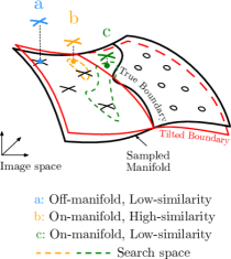
Figure 1: Our interpretation of zeroth-order attack behavior in the context of boundary tilting (Tanay & Griffin, 2016): a) zeroth-order attack targeting low-level features, leaving the manifold, b) an efficient zeroth-order attack targeting mostly high-level features, floating along the manifold, and c) manifold-based zeroth-order attack next to the manifold, but sacrificing similarity. For example, in our evaluation a, b, and c would correspond to Sign-OPT, BiLN+Sign-OPT, and AE+Sign-OPT, respectively.

Despite the steady improvements of hard-label attacks, open questions persist about their behavior, and AML attacks at large. Adversarial samples were originally assumed to lie in rare pockets of the input space (Goodfellow et al., 2014), but this assumptions was later challenged by the boundary tilting assumption (Tanay & Griffin, 2016; Gilmer et al., 2018), which adopts a “data-geometric” view of the input space living on a lower-dimensional manifold. This is supported by Stutz et al. (2019), who suggest that regular adversarial examples leave the data manifold, while on-manifold adversarial examples are generalization errors. From a data-geometric perspective, a sample’s distance to the manifold primarily describes the amount of semantic features preserved during the attack process. This makes it advantageous to produce on-manifold adversarial examples, since the adversary can exploit the inherent generalization error of the model, while producing samples that are semantically similar. However, the true data manifold is either difficult or impossible to describe, and relying solely on approximations of the manifold can lead to the creation of crude adversarial examples (Stutz et al., 2019).

In this paper, we adopt the boundary-tilting assumption and demonstrate an unexpected benefit of query-efficient zeroth order attacks, i.e., attacks primarily enabled by the use of down-scaling techniques. These attacks are more likely to discover on-manifold examples, which we argue is the result of manifold-gradient mutual information. While seemingly counter-intuitive, since down-scaling techniques reduce the search dimension (artificially limiting the search space for adversarial examples), our results suggest that the manifold-gradient mutual information can actually increase as a function of the effective dimensionality, and number of training points. This behavior leads to examples that are on-manifold generalization errors. With this knowledge, it is possible to rethink the design of hard-label attacks, to target high-level features as in attack (b) in Figure 1, rather than (a) or (c).

Our specific contributions are as follows:

• Introduction of manifold distance oracle. To create on-manifold examples, the adversary must leverage manifold information during the attack phase. We thus propose an information-theoretical formulation of the noisy manifold distance (NMD) oracle, which can explain how zeroth-order attacks craft on-manifold examples. We experimentally demonstrate that manifold-gradient mutual information can increase as a function of the effective problem dimensionality and number of training points. This finding relates to known behavior in the gradient-level setting, where manifold information can be leaked from robust models (Engstrom et al., 2019); unlike that work, however, our formulation describes leakage from both natural and robust models.

• Reveal new insights of manifold feedback during query-efficient zeroth-order search. We describe an approach for extending dimension-reduction techniques in the score-level setting (Tu et al., 2019) to hard-label attacks. We propose the use of FID score (Heusel et al., 2018) as an $L_{p}$-agnostic means for estimating the adversary’s manifold information gain. This methodology allows us to empirically demonstrate the connection between dimension reduction and manifold feedback from the model, beyond the known convergence rates tied to dimensionality (Nesterov & Spokoiny, 2017).

• Attack-agnostic method for super-pixel grouping. We show that bilinear down-scaling of the input space act as a form of super-pixel grouping, yielding up to 28% and 76% query efficiency gain for previously-proposed HSJA (Chen et al., 2019) and Sign-OPT attacks (Cheng et al., 2020), respectively against robust models.More importantly, we show that super-pixel grouping produces samples close to the manifold and exploits the inherent generalization error of the model.

2 Related Work

Since the original discovery of adversarial samples against deep models (Szegedy et al., 2013; Goodfellow et al., 2014), the prevailing question was why such examples existed. The original assumption was that adversarial examples lived in low-probability pockets of the input space, and were never encountered during parameter optimization (Szegedy et al., 2013). This effect was believed to be amplified by the linearity of weight activations in the presence of small perturbations (Goodfellow et al., 2014). These assumptions were later challenged by the manifold assumption, which in summary 1) asserts that the train and test sets of a model only occupy a sub-manifold of the true data, while the decision boundary lies close to samples on and beyond the sub-manifold (Tanay & Griffin, 2016), and 2) supports the “data geometric“ view, where high-dimensional geometry of the true data manifold enables a low-probability error set to exist (Gilmer et al., 2018). Likewise the manifold assumption describes adversarial samples as leaving the manifold, which has inspired defenses based on projecting such samples back to the data manifold (Jalal et al., 2019; Samangouei et al., 2018). However, these approaches were later defeated by adaptive attacks (Carlini et al., 2019; Carlini & Wagner, 2017; Tramer et al., 2020). We investigate the scenario where an adversary uses zeroth-order information to estimate the desired gradient direction (Cheng et al., 2020; Chen et al., 2019). Thus the adversary uses only the top-1 label feedback from their model query to synthesize samples. The desire for better query efficiency motivated the use of dimension reduction in hard-label attacks. However, to date it is not completely understood how this relates to traversal through the data manifold. We leverage previous results of the gradient-level setting (Stutz et al., 2019; Engstrom et al., 2019) to formulate an explanation of manifold leakage during hard-label adversarial attacks.

3 Noisy Manifold Distance Oracle

Santurkar et al. (2019) demonstrate that the gradients of robust models have higher visual semantic alignment with the data compared to gradients of standard models. This suggests a reduction in uncertainty when sampling from the distribution of visual perturbations. If this reduced uncertainty can be attributed to leaked knowledge of the original data manifold, an adversary could exploit this fact and produce samples closer to the manifold.

This connects to the hard-label setting as follows. First, recall a standard result in data processing, which states that if three random variables form the Markov chain ${\displaystyle X\rightarrow Y\rightarrow Z}$, then their mutual information (MI) has the relation ${\displaystyle I(X;Y)\geqslant I(X;Z)}$ (Beaudry & Renner, 2012). Now we have the data manifold $\mathcal{M}=X$, the input gradient $\mathcal{G}=Y$, and the noisy gradient from the black-box hard-label attack as $\ddot{\mathcal{G}}=Z$. If $I(\mathcal{M},\mathcal{G})$ is larger for adversarially robust models, this may also suggest $I(\mathcal{M},\ddot{\mathcal{G}})$ is larger. In the information theoretic sense, does this mean the gradients of adversarially robust models reveal more information about the training data than standard models? An immediate follow-up concern is whether other factors can influence the model to reveal this information, such as the problem dimensionality. Schmidt et al. (2018) have shown that robust training requires additional data as a function of the data dimensionality. To test this hypothesis, we leverage the data model and results from  Schmidt et al. (2018) to derive an analytical solution for $I(\mathcal{G},\mathcal{M})$. This allows us to estimate the mutual information gain (or lack thereof) from adding extra training samples, as is the case in the adversarially robust setting, or reducing the effective problem dimensionality, as is common for hard-label attacks.

Data model and weights.

Recall the Gaussian mixture data model from Schmidt et al. (2018):

Definition 3.1.

(Gaussian model). Let $\boldsymbol{\theta}*\in\mathbb{R}^{d}$ be the per-class mean vector and let $\sigma>0$ be the variance parameter. Then the $(\boldsymbol{\theta}*,\sigma)$-Gaussian model is defined by the following distribution over $(\mathbf{x},y)\in\mathbb{R}^{d}\times\{\pm 1\}$: First, draw a label $y\in\{\pm 1\}$ uniformly at random. Then sample the data point $\mathbf{x}\in\mathbb{R}^{d}$ from $\mathcal{N}(y\cdot\boldsymbol{\theta}*,\sigma^{2}I)$.

The difficulty of classification (i.e., linear separability) is controlled by the parameter $\sigma^{2}$ since we maintain $||\boldsymbol{\theta}^{*}||\simeq\sqrt{d}$. The data manifold is paramaterized for the Gaussian model by $(\boldsymbol{\theta}^{*},\sigma)$.

Next, recall a standard definition of classification error.

Definition 3.2.

(Classification error). Let $\mathcal{P}:\mathbb{R}^{d}\times\{\pm 1\}\rightarrow\mathbb{R}$ be a distribution. Then the classification error $\beta$ of a classifier $f:\mathbb{R}^{d}\rightarrow\{\pm 1\}$ is defined as $\beta=\mathbb{P}_{(\mathbf{x},y)\sim\mathcal{P}}[f(\mathbf{x})\neq y]$.

Optimal classification weight (non-robust): Fix the $(\boldsymbol{\theta}^{*},\sigma)$-Gaussian model with $||\boldsymbol{\theta}^{*}||_{2}=\sqrt{d}$ and $\sigma\leq c\cdot d^{\frac{1}{4}}$, where c is a universal constant. Schmidt et al. (2018) prove that for the linear classifier $f_{\mathbf{w}}:\mathbb{R}^{d}\rightarrow\{\pm 1\}$ defined as $f_{\mathbf{w}}(x)=\text{sgn}(\mathbf{w}\cdot\mathbf{x})$, setting $\widehat{\mathbf{w}}=y\cdot\mathbf{x}$ (using a single tuple from the distribution) yields a linear classifier $f_{\widehat{\mathbf{w}}}$ with classification error of at most 1%, with high probability.

Schmidt et al. (2018) later define a notion of robust classification error based on a bounded worst-case perturbation of input samples, which we defer to their paper for reference.

Optimal classification weight (robust).

Now fix $\sigma\leq c_{1}d^{\frac{1}{4}}$ for the universal constant $c_{1}$, and samples $(x_{1},y_{1}),\cdots,(x_{n},y_{n})$ drawn $i.i.d$ from the $(\boldsymbol{\theta}^{*},\sigma)$-Gaussian model with $||\boldsymbol{\theta}^{*}||=\sqrt{d}$. Schmidt et al. (2018) prove that the weight setting $\widehat{w}=\frac{1}{n}\sum^{n}_{i=1}y_{i}x_{i}$ yields an $l^{\epsilon}_{\infty}$-robust classification error of at most 1% for the linear classifier $f_{\widehat{w}}$ if

$$n\geq\begin{cases}1,&\text{for }\leavevmode\nobreak\ \epsilon\leq\frac{1}{4}d^{-\frac{1}{4}}\\ c_{2}\epsilon^{2}\sqrt{d},&\text{for }\leavevmode\nobreak\ \frac{1}{4}d^{-\frac{1}{4}}\leq\epsilon\leq\frac{1}{4}\end{cases},$$ (1)

for a universal constant $c_{2}$. We can leverage the weight settings as a function of $n$ and $d$ to give a closed form solution of mutual information.

3.1 Gradient-Manifold Mutual Information (MI)

For simplicity fix $d=1$. Notice the classifier $\text{sgn}(\cdot)$ is discontinuous at $x=0$. Instead we consider the sub-gradient of the classifier at $x<0$ and $x>0$. In either case (non-robust or robust), the input sub-gradient for $f_{\widehat{w}}(x^{\prime})$ is defined as $\nabla_{x^{\prime}}f_{\widehat{w}}=\text{sgn}(\widehat{w})$. Since the weights are Gaussian distributed with $\widehat{w}\sim\mathcal{N}(\boldsymbol{\theta}^{*},\sigma)$, we can define the distribution of gradients as $\mathcal{G}\sim\text{Bernoulli}\left(\mathbb{P}_{\widehat{w}\sim\mathcal{N}}\left[\widehat{w}\geq 0\right]\right)$. This allows defining the manifold-gradient point-wise joint probabilities case-wise, for the respective values under $g$ and $x$. We are concerned with the sub-gradient cases where $x>0$ (denoted $x^{+}$) and $x<0$ (denoted $x^{-}$) which correspond to the fixed values $g\in\{-1,1\}$.

Using the standard definition of the Gaussian distribution for both gradient and manifold, we can derive a closed form solution for the manifold-gradient mutual information (MI). The complete derivation of the joint and marginal probabilities can be found in Section B of the Appendix. We leverage Riemann approximation of the Gaussians over finite distance $\Delta_{i}=x_{i}-x_{i-1}$ for positive points in the Gaussian distribution $x_{i}^{*}\in[x_{i-1},x_{i}]$, where $i\in\{1,\ldots,n\}$.

Fix $\sigma=cd^{\frac{1}{4}}$ for the non-robust case and $\sigma=c_{1}d^{\frac{1}{4}}$ for the robust case. We denote the sub-manifold sampled from the positive ($y=1$) and negative ($y=-1$) classes as $\mathcal{M}^{+}$ and $\mathcal{M}^{-}$, respectively. After simplifying due to symmetry, we have the closed form solution of manifold-gradient mutual information, based on the standard definition of mutual information from information theory (Cover & Thomas, 2006),

$$I(\mathcal{G},\mathcal{M})_{\epsilon} =2\int_{\mathcal{M}^{+}}p(1,x^{+})\,\text{log}(\frac{p(1,x^{+})}{p_{\mathcal{G}}(1)p_{\mathcal{M}}(x^{+})})\,dx^{+}+2\int_{\mathcal{M}^{+}}p(-1,x^{+})\,\text{log}(\frac{p(-1,x^{+})}{p_{\mathcal{G}}(-1)p_{\mathcal{M}}(x^{+})})\,dx^{+}.$$ (2)

This leads to the Riemann approximation of Equation 2 used in numerical experiments as

$$I(\mathcal{G},\mathcal{M})_{\epsilon} =\frac{2}{\sqrt{2\pi}\sigma^{2}}\sum^{||\mathcal{M}^{+}||}_{i=1}\text{exp}(-\frac{(x_{i}^{*}-\theta)^{2}}{2\sigma^{2}})\cdot\beta^{+}_{i}\Delta_{i}+\frac{2}{\sqrt{2\pi}\sigma^{2}}\sum^{||\mathcal{M}^{+}||}_{i=1}\text{exp}(-\frac{(x_{i}^{*}+\theta)^{2}}{2\sigma^{2}})\cdot\beta^{-}_{i}\Delta_{i}.$$ (3)

where

$$\beta^{+}_{i} =-\frac{(x_{i}^{*}-\theta)^{2}}{2\sigma^{2}}-\text{log}(\lambda_{+})-\text{log}\left(\text{exp}(-\frac{(x_{i}^{*}-\theta)^{2}}{\sigma^{2}})+\text{exp}(-\frac{(x_{i}^{*}+\theta)^{2}}{\sigma^{2}})\right),$$ (4)

$$\beta^{-}_{i} =-\frac{(x_{i}^{*}+\theta)^{2}}{2\sigma^{2}}-\text{log}(\lambda_{-})-\text{log}\left(\text{exp}(-\frac{(x_{i}^{*}-\theta)^{2}}{\sigma^{2}})+\text{exp}(-\frac{(x_{i}^{*}+\theta)^{2}}{\sigma^{2}})\right),$$

$$\lambda_{+} =\frac{1}{\sqrt{2\pi}\sigma}\sum_{j=1}^{n}\text{exp}\left({-\frac{1}{2}\cdot\frac{(x_{j}^{*}-\theta)^{2}}{\sigma^{2}}}\right)\Delta_{i},$$

$$\lambda_{-} =\frac{1}{\sqrt{2\pi}\sigma}\sum_{j=1}^{n}\text{exp}\left({-\frac{1}{2}\cdot\frac{(x_{j}^{*}+\theta)^{2}}{\sigma^{2}}}\right)\Delta_{i},$$

for $\Delta_{i}=x_{i}-x_{i-1}$, positive $x_{i}^{*}\in[x_{i-1},x_{i}]$ and $x_{j}^{*}\in[x_{j-1},x_{j}]$. The values $\lambda_{+}$ and $\lambda_{-}$ resolve to the Riemann approximation of the marginal probabilities for $g=1$ and $g=-1$, respectively ($n$ given by $(\epsilon,d)$ setting). The $(\epsilon,d)$ setting determines the $n$ independent draws from the manifold for calculating the gradient marginal.

3.2 Mutual information as a function of dimensionality

Recall that $d$ controls $\sigma$ in Equation 3, i.e., $\sigma=cd^{\frac{1}{4}}$ for non-robust case and $\sigma=c_{1}d^{\frac{1}{4}}$ for robust case. This represents a constant fraction of the probability mass in Equation 3, which causes the mutual information to vary with $d$. To study this further, we run numerical experiments to estimate $I(\mathcal{G},\mathcal{M})$ as derived in Equation 3, while varying the dimensionality $d$ against values of $c_{2}\in\{1,5,10,15\}$ and $\epsilon\in\{0.0,0.125,0.250\}$. Notice that the universal constant $c_{2}$ for robust weight setting controls the scaling of training points in Equation 1, while $c$ and $c_{1}$ scale the allowed variance as a function of $d$. This means that $c$ and $c_{1}$ can be fixed (we use $0.5$) while $c_{2}$ and $d$ can be changed to study their effect. As in the data model presented earlier, we assume dimension co-independence, i.e., the covariance matrix $\mathbf{\Sigma}=\sigma I$. We also assume the manifold can be described with $n$ points, i.e., $||\mathcal{M}||=n$ defined by Equation 1.

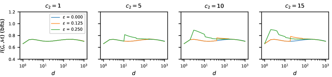
Figure 2: a) Mutual information (MI) over dimension $d$ for several values of $c_{2}$ and $\epsilon$ in Equation 2, log-scale $d$-axis with $d\in[1,10^{3}]$. The MI is higher at lower $d$ when $c_{2}$ (# of training points) is increased w.r.t $d$, and when perturbation size $\epsilon$ is greater.

The result of estimation is shown in Figure 2 with log-scale x-axis. When $c_{2}=1$, increased $\epsilon$ produces no change in mutual information. However, setting $c_{2}$ to higher values allows for higher mutual information from increased $\epsilon$. The effect is noticeable through to $c_{2}=15$. Given sufficient scaling factor $c_{2}$, mutual information increases reliably for lower dimension $d$. This effect is most noticeable when $\epsilon=0.25$ (green line). That is, given a sufficient surplus in training points, a robust model could act as an oracle leaking information through over-specification, i.e., include too many training points, or when the effective dimensionality of the learning problem is reduced. This can theoretically explain the high visual alignment observed empirically by Engstrom et al. (2019) and Santurkar et al. (2019) on robust models. From an evasion adversary’s perspective, the model cannot be modified to become over-specified, so this axis of mutual information gain is left for future work. Instead, we focus on the effective dimensionality, which the adversary can control through manifold-descriptive queries to the model, as it relates to higher values of $\epsilon$ in robust models.

4 Zeroth-order search through the manifold distance oracle

We showed from an information theoretic view that the true gradient during a black-box attack can act as a manifold distance oracle, and this oracle leaks more information based on the effective dimension of the learning problem. As a result, high MI between the true gradient and data manifold would suggest more information leakage between a noisy gradient estimate and the data manifold. We now investigate this phenomena in the context of real-world datasets. In the most common problem setting, the adversary is interested in attacking a $K$-way multi-class classification model $f:\mathbb{R}^{d}\to\{1,\dots,K\}$. Given an original example $\mathbf{x}_{0}$, the goal is to generate adversarial example $\mathbf{x}$ such that $\mathbf{x}\text{ is close to }\mathbf{x}_{0}\text{ and }f(\mathbf{x})\neq f(\mathbf{x}_{0}),$ where closeness is often approximated by the $L_{p}$-norm of $\mathbf{x}-\mathbf{x}_{0}$. The value of this approximation is debated in the literature (Heusel et al., 2018; Tsipras et al., 2018; Engstrom et al., 2019). We turn to alternative methods shown later for measuring closeness. First we step through the formulation for contemporary hard-label attacks, then show how dimension-reduced attacks can be formulated in the hard-label setting, which enables empirical analysis of our theoretical result.

4.1 Gradient-level formulation

For gradient-level attacks, the goal is satisfied by first assuming that $f(\mathbf{x})=\text{argmax}_{i}(Z(\mathbf{x})_{i})$, where $Z(\mathbf{x})\in\mathbb{R}^{K}$ is the final (logit) layer output, and $Z(\mathbf{x})_{i}$ is the prediction score for the $i$-th class, the stated goal is satisfied by the optimization problem,

$$h(\mathbf{x}):=\underset{\mathbf{x}}{\operatorname{\text{argmin}}}\left\{||\mathbf{x}-\mathbf{x}_{0}||_{p}+c\mathcal{L}(Z(\mathbf{x}))\right\}$$ (5)

for the Euclidean $L_{p}$-norm $||\cdot||_{p}$, the loss function corresponding to the goal of the attack $\mathcal{L}(\cdot)$, and a regularization parameter $c$. A popular choice of loss function is the Carlini & Wagner (2016) loss function.

4.2 Score-level and hard-label attacks

In the gradient-level setting, we require the gradient $\nabla f(\cdot)$. However, in the score-level setting we are forced to estimate $\frac{\partial f(\mathbf{x})}{\partial\mathbf{x}}$ without access to $\nabla f(\cdot)$, only evaluations of $Z(\cdot)$. Tu et al. (2019) reformulate the previous problem to a version relying instead on the ranking of class predictions from $Z$. In practical scenarios, the estimate is found using random gradient-free method (RGF), a scaled random full gradient estimator of $\nabla f(\mathbf{x})$, over $q$ random directions $\{\mathbf{u}_{i}\}^{q}_{i=1}$. The score-level setting was extended to several renditions of the hard-label setting, which we clarify below. In each case the goal is to approximate the gradient by $\hat{\mathbf{g}}$.

OPT-Attack

For given example $\mathbf{x}_{0}$, true label $y_{0}$, and hard-label black-box function $f:\mathbb{R}^{d}\to\{1,\dots,K\}$, Cheng et al. (2019) define the objective function $g:\mathbb{R}^{d}\to\mathbb{R}$ as a function of search direction $\boldsymbol{\theta}$, where $g(\boldsymbol{\theta}^{*})$ is the minimum distance from $\mathbf{x}_{0}$ to the nearest adversarial example along the direction $\boldsymbol{\theta}$. For the untargeted attack, $g(\boldsymbol{\theta})$ corresponds to the distance to the decision boundary along direction $\boldsymbol{\theta}$, and allows for estimating the gradient as

$$\hat{\mathbf{g}}=\frac{1}{q}\sum^{q}_{i=0}\frac{g(\boldsymbol{\theta}+\beta\mathbf{u}_{i})-g(\boldsymbol{\theta})}{\beta}\cdot\mathbf{u}_{i},$$ (6)

where $\beta$ is a small smoothing parameter. Notably, $g(\boldsymbol{\theta})$ is continuous even if $f$ is a non-continuous step function.

Sign-OPT

Cheng et al. (2020) later improved the query efficiency by only considering the sign of the gradient estimate,

$$\hat{\nabla}g(\boldsymbol{\theta})\approx\hat{\mathbf{g}}:=\sum_{i=1}^{q}\text{sgn}\left(g(\boldsymbol{\theta}+\beta\mathbf{u}_{i})-g(\boldsymbol{\theta})\right)\mathbf{u}_{i}.$$

We focus on the Sign-OPT variant, since the findings are more relevant to the current state-of-the-art.

HopSkipJumpAttack

Similar to Sign-OPT, HopSkipJumpAttack (HSJA) (Chen et al., 2019) uses a zeroth-order sign oracle to improve Boundary Attack (Brendel et al., 2017). HSJA lacks the convergence analysis of OPT Attack/Sign-OPT and relies on one-point gradient estimate. Regardless, HSJA is competitive with Sign-OPT for state-of-the-art in the $L_{2}$ setting.

Alternative hard-label attacks exist which do not rely on the explicit zeroth-order gradient estimate from the model, such as RayS by Chen & Gu (2020). We expect such attacks to behave differently, and thus provide results for RayS in Section D.2 of the Appendix.

4.3 Dimension-reduced zeroth-order search

In order to characterize hard-label attacks against the MI to dimension relationship shown in Section 3.2, we modify existing hard-label attacks to produce dimension-reduced variants. This scheme can allow dynamic scaling of the effective dimensionality up or down in a controlled manner. Our dimension-reduced search is feasible since the intrinsic dimensionality of data can be lower than the true dimension (Amsaleg et al., 2017). In practice we implement the reduction through an encoding map $\mathcal{E}:\mathbb{R}^{d}\to\mathbb{R}^{d^{\prime}}$ for reduced dimension $d^{\prime}$ and decoding map $\mathcal{D}:\mathbb{R}^{d^{\prime}}\to\mathbb{R}^{d}$. In general the adversarial sample is created by

$$\mathbf{x}=\mathbf{x}_{0}+g\left(\mathcal{D}(\boldsymbol{\theta}^{\prime})\right)\frac{\mathcal{D}(\boldsymbol{\theta}^{\prime})}{||\mathcal{D}(\boldsymbol{\theta}^{\prime})||},$$ (7)

where $\boldsymbol{\theta}^{\prime}\in\mathbb{R}^{d^{\prime}}$ and is optimized depending on the respective attack (e.g., Sign-OPT and HSJA), and as before, $g$ is a measure of distance to the decision boundary in direction $\mathcal{D}(\boldsymbol{\theta}^{\prime})$. The mapping functions can be initialized with either an autoencoder (AE), or a pair of channel-wise bilinear transform functions (henceforth referred to as BiLN) which simply scales the input up or down depending on a fixed scaling factor. This represents two distinct methods of synthesizing adversarial samples, which either rely on an approximate description of the manifold (AE), or instead exploit the known spatial codependence of images (BiLN).

The adversary’s AE is tuned to minimize reconstruction error of input images, so the output quality of the AE will depend on the adversary’s ability to collect data. We assume the adversary only has access to the test set, which tends to be considerably less informative than the training set. This crude manifold approximation can manifest as an additional layer of distortion on top of adversarial noise. With BiLN, no additional training is required, so it synthesizes search directions independent of the adversary’s manifold description (i.e., possible extracted knowledge about test samples). The complete implementation details of the AE variant can be found in Section C of the Appendix. Next we describe how the mapping functions are used in our experiments.

Sign-OPT & HSJA.

In general, for attacks relying on the Cheng et al. (2019) formulation, the update in Equation 6 becomes

$$\hat{\mathbf{g}}=\frac{1}{q}\sum^{q}_{i=0}\frac{g(\boldsymbol{\theta}^{\prime}+\beta\mathbf{u}^{\prime}_{i})-g(\boldsymbol{\theta}^{\prime})}{\beta}\cdot\mathbf{u}^{\prime}_{i}$$ (8)

for the reduced-dimension Gaussian vectors $\{\mathbf{u}^{\prime}_{i}\in\mathbb{R}^{d^{\prime}}\}_{i=0}^{q}$ for integer $d^{\prime}<d$ and direction $\boldsymbol{\theta}^{\prime}\in\mathbb{R}^{d^{\prime}}$. The reduced-dimension direction $\boldsymbol{\theta}^{\prime}$ is initialized randomly with $\boldsymbol{\theta}^{\prime}\sim\mathcal{N}(0,1)$ for the untargeted case, or for the targeted case as $\boldsymbol{\theta}^{\prime}=\mathcal{E}(\mathbf{x}_{t})$, where $\mathbf{x}_{t}$ is a test sample correctly classified as target class $t$ by the victim model. This scheme also applies to HSJA, since HSJA performs a single-point sign estimate. As in the normal variants, $\hat{\mathbf{g}}$ is used to update $\boldsymbol{\theta}^{\prime}$.

4.4 Estimating manifold-gradient mutual information

We can leverage a sample’s distance to the manifold as a signal of the effective gradient-manifold mutual information. Hereafter, we refer to this distance w.l.o.g as the manifold distance. Unfortunately, the real data manifold is difficult to describe. This is an open problem in the study of Generative Adversarial Networks (GANs), since designers require that generator images are on-manifold to preserve semantic relationships between images. This has motivated the recently proposed Fréchet Inception Distance (FID) that acts as a surrogate measure of the manifold distance (Heusel et al., 2018). We can leverage FID by treating the adversarial samples as synthetically generated images, which are later compared to their unmodified counterparts on the true manifold. Since FID uses an Inception-V3 coding layer (Szegedy et al., 2016) to encode images, this distance correlates with distortion of semantic high-level features. Thus sampling closer to the data manifold will result in a lower FID score. We do not target the Inception-V3 network in any of our experiments, so the FID metric will not rely on any internal aspects of the victim models.

5 Results

5.1 Methodology

Our experimental analysis addresses the following three research questions about zeroth-order attacks:

1. Under the analytical result of Section 3.2, does the adversary take advantage of increased manifold-gradient mutual information in practice?

2. Similarly, is manifold-gradient mutual information affected by the model robustness?

3. If the dimension is reduced as in Figure 2, what is the trade-off between query efficiency and the resulting reduced search resolution?

We study these questions by comparing two hard-label attacks with their compatible dimension-reduced variants, against both natural and robust models. The robust models contain an improved loss landscape as a result of increased sample complexity during the training or inference process.

Experimental Highlights.

Our experiments show that query-efficient attacks exhibit unexpected behaviors and benefits, with explanations summarized below:

1. Query-efficient gradient estimates reduce the effective dimensionality of the adversary’s search. In experiments against CIFAR-10, this increases manifold-gradient mutual information, which allows lower FID-64 scores for BiLN+HSJA, BiLN+Sign-OPT, and AE+Sign-OPT.

2. Robust models increase the sample complexity during training, which creates a cleaner loss landscape. Although we observe high FID-64 scores on the robust Madry model using normal attacks, dimension-reduction allows to match the low baseline scores of the natural model.

3. Dimension-reduced attacks are capable of state-of-the-art query-efficiency gains for HSJA and Sign-OPT against robust models, despite reducing the effective search resolution.

Setup.

All attacks run for 25k queries without early stopping. For brevity, we only show results for the untargeted case. FID score is calculated using the 64-dimensional max pooling layer of the Inception-V3 deep network for coding (denoted as FID-64), taken from an open-source implementation. The choice of the 64-dimensional feature layer allows to calculate full-rank FID without the full 2,048 sample count of original FID, which is prohibitive based on the scale of our analysis. Since the coding layer differs slightly from the original FID-2048 implementation, the magnitudes will differ from those published by Heusel et al. (2018).

Image data consists of the CIFAR-10 (Krizhevsky, 2009) classification dataset. Original samples are chosen from the test set using the technique from Chen et al. (2019): on CIFAR-10, ten random samples are taken from each of ten classes (i.e., 100 total samples). The natural CIFAR-10 network is the same implementation open-sourced by Cheng et al. (2020). In addition, we leverage the representative adversarial training technique proposed by Madry et al. (2017) (and their checkpoint) as the robust model. Additional results on the ImageNet dataset (Russakovsky et al., 2015) can be found in Section D.1 of the Appendix. To avoid ambiguity, we label each BiLN variant with the spatial dimension after performing the bilinear transformation.

5.2 Experimental details

We target the $L_{p}$-norm which the robust model was regularized under, i.e., $L_{\infty}$ versions of the attacks for CIFAR-10.

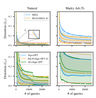
(a)

(b)

Figure 3: Results across attacks for CIFAR-10 dataset, corresponding to a) distortion against query usage (dotted red line denotes the value of $\epsilon$, shaded areas mark standard deviation), and b) FID-64 trajectory against the same query usage. The estimate of manifold-gradient mutual information (FID-64) is universally lower on dimension-reduced attacks, such as BiLN and AE variants.

CIFAR-10 case study ($L_{\infty})$.

We measure the distortion against remaining query budget of the adversary in Figure 3a. In general, the normal variants of each attack align with the published results. The main improvement is with BiLN+HSJA (orange line, top row) against the Madry adversarial training model, with average distortion at 4k queries decreasing from 0.09 to 0.07. This improvement is contrary to the minimal effect on the natural model (Inset 3a.i blue line). AE+Sign-OPT (green line, bottom row) outperforms against regular Sign-OPT (blue line) and BiLN+Sign-OPT (orange line) on the robust model. However, the success with AE+Sign-OPT tends to be situational; in practice the low quality of the AE manifold description does not permit fine-grained adjustments to the perturbation. Overall, the Madry model could be weak against the zeroth-order distortions, since their formulation only considers first-order adversaries Madry et al. (2017). To accompany the distortion results, we provide success rate plots for CIFAR-10 in Section D.3 of the Appendix.

Our next focus is Figure 3b, which shows the FID score’s trajectory over the search queries. Every trajectory will begin at a zero value, since there is an expected score of zero for identical images, and then peaks as the attack initialization is performed. Our main observation is the decrease in FID-64 score using the dimension-reduced variants. The magnitudes for AE+Sign-OPT (green line, Inset 3b.ii) peaks at 0.28, then falls (and stays) near 0.004. BiLN+HSJA and BiLN+Sign-OPT (orange lines of Insets 3b.i and 3b.ii) both exhibit lower FID scores than their normal variants (blue lines), as much as two orders of magnitude less in the case of BiLN+Sign-OPT. The reduced dimensionality leads to a lower FID-64 score, i.e., greater manifold information through the gradient estimate. On the Madry Adv. Tr. robust model (right column), we see a universal behavior where dimension-reduced variants produce a large reduction of FID-64 score. On Sign-OPT variants (bottom row), dimension reduction produces FID-64 score matching the baseline scores of the natural model. As a result, we can conclude that manifold information leakage occurs regardless of model sample complexity, and improves under certain dimension reduction schemes, such as BiLN+Sign-OPT and AE+Sign-OPT. We expand on this result in the next section. For completeness, we provide visual and tabular evidence of this behavior in Sections D.5 and  D.4 of the Appendix, respectively.

6 Discussion

Evidence of the noisy manifold distance oracle.

From an information-theoretical perspective, the zeroth-order adversary observes the noisy manifold distance (NMD), which is leaked as side information by each gradient estimate. Against the natural model, dimension-reduced attacks led to a straightforward reduction in FID-64 score, as suggested by the numerical results of Section 3.2. Against the robust Madry model, normal attack variants had an inflated FID-64 score. However, BiLN+Sign-OPT and AE+Sign-OPT ultimately matched the baseline scores of the natural model. This suggests the NMD oracle improved in conjunction with the loss landscape of the victim model. This follows the data processing inequality (DPI) (Beaudry & Renner, 2012): if $\textsc{I}(\mathcal{M},\mathcal{G})$ increases, then $\textsc{I}(\mathcal{M},\ddot{\mathcal{G}})$ also increases, where $\mathcal{M}$ is the manifold, and $\ddot{\mathcal{M}}$ is the noisy gradient. In words, the quality of the noisy gradient depends on the quality of the model’s loss landscape, which can more closely resemble the manifold under robust regularization. This means a higher quality loss landscape leads to a higher quality zeroth-order attack. As we showed in Section 3, this result is closely tied to the effective dimensionality, which can be arbitrarily lower than the true dimensionality Ma et al. (2018).

	Gradient Deviation
Attack Variant	$||\mathbf{g}-\hat{\mathbf{g}}||_{\infty}$	$||\mathbf{g}-\hat{\mathbf{g}}||_{2}$
Sign-OPT	4.154 $\pm$ 1.127	40.728 $\pm$ 9.166
Sign-OPT+BiLN	4.067 $\pm$ 1.252	40.643 $\pm$ 11.039
Sign-OPT+AE	4.373 $\pm$ 1.118	49.587 $\pm$ 9.194
HSJA	4.884 $\pm$ 1.208	69.295 $\pm$ 6.332
HSJA+BiLN	4.584 $\pm$ 1.048	55.901 $\pm$ 6.963

Table 1: Comparison of the deviation between the true gradient and the first gradient estimate from various hard-label attack variants, in the direction of the successful adversarial prediction, averaged over 50 samples on CIFAR-10.

Effect on gradient deviation.

When measuring FID-64 score, the score for BiLN+HSJA on the robust model failed to match the natural score, despite outperforming in distortion. A notable difference between HSJA and Sign-OPT (apart from analytic guarantees) is the method for performing estimates, e.g., one-point with HSJA and two-point for Sign-OPT. Liu et al. (2020) showed that the one-point method can be noisier, which according to DPI will restrict the mutual information. We hypothesize that the one-point approach also leaves the manifold sooner, due to updating the reference sample on-the-fly. To quantify this, we calculate the $L_{\infty}$-norm and $L_{2}$-norm between the first gradient estimate for each attack variant and the true input gradient. The true input gradient is calculated from the original sample with respect to the cross-entropy loss between the model output and classification label of the adversarial sample. This comparison is shown in Table 1 for the natural CIFAR-10 model, averaged over 50 samples from each attack. Sign-OPT variants have a universally lower gradient deviation than the HSJA variants. Notably, the Sign-OPT+BiLN variant (bolded) obtains the lowest gradient deviation, whereas HSJA has the highest deviation. These observations support our empirical argument that HSJA leads to a higher FID score, due to a higher variance in the gradient estimate as shown before by Liu et al. (2020). The larger gradient deviation for HSJA implies noisier gradient estimation, and hence by the data processing inequality (DPI) leads to a lower mutual information (MI) between the data manifold and noisy gradients.

“Topology” of hard-label settings.

We can view zeroth-order attacks as following a topological hierarchy that is a function of the effective data dimension. Our interpretation is illustrated in Figure 1. Each technique offers a unique traversal distance both along the manifold, and away from it. Efficient attacks represented by (b) can combine elements of staying near manifold, and traversing it. This is representative of BiLN variants, which make basic assumptions about spatial correlation to balance search fidelity with manifold distance. In contrast, traversing close to an approximate manifold description with (c) introduces distortion as a result of the crude manifold description. Following the boundary tilting assumption, the nearest boundary on the manifold could also be far away. Thus we can consider an attack which learns a manifold description (e.g., an AE variant), but instead leverages the description to select the most relevant super-pixel grouping in the image. To this end, the FID score offers a reliable measure of manifold distance, which can inform the topological behavior, and the quality of future hard-label attacks. This ultimately enables a better evaluation of model robustness.

7 Conclusion

Despite the recent progress in zeroth-order attack methods, open questions remain about their precise behavior. We develop an information-theoretic analysis that sheds light on their ability to produce on-manifold adversarial examples as a function of effective dimensionality. Through experiments on real-world datasets, we show up to two-fold decrease in the manifold distance by leveraging dimension-reduced attack variants. With knowledge of the manifold-gradient relationship, it is possible to further refine hard-label attacks, and inform a better evaluation of model robustness.

Appendix A Appendix

Appendix B Derivation of Manifold-Gradient Mutual Information (MI)

We define the manifold-gradient point-wise joint probability in a case-wise manner, for the respective values under $g$ and $x$. We are concerned with the sub-gradient cases where $x>0$ (denoted $x^{+}$) and $x<0$ (denoted $x^{-}$) which correspond to fixed values of $g$. This gives

$$p(g=1,x^{+}) =\frac{1}{2\sqrt{2\pi}\sigma}\text{exp}\left({-\frac{1}{2}\cdot\frac{(x^{+}-\theta)^{2}}{\sigma^{2}}}\right)$$ (9)

$$p(g=1,x^{-}) =\frac{1}{2\sqrt{2\pi}\sigma}\text{exp}\left({-\frac{1}{2}\cdot\frac{(x^{-}+\theta)^{2}}{\sigma^{2}}}\right)\,,$$

$$p(g=-1,x^{+}) =\frac{1}{2\sqrt{2\pi}\sigma}\text{exp}\left({-\frac{1}{2}\cdot\frac{(x^{+}+\theta)^{2}}{\sigma^{2}}}\right)$$ (10)

$$p(g=-1,x^{-}) =\frac{1}{2\sqrt{2\pi}\sigma}\text{exp}\left({-\frac{1}{2}\cdot\frac{(x^{-}-\theta)^{2}}{\sigma^{2}}}\right)\,.$$

Since the Schmidt et al. Gaussian mixture is created symmetrically (the probability mass is evenly split between the two classes i.e., the mixture comprises one Gaussian offset by $\theta$ and mirrored at $x=0$) we can simplify to

$$p(g=1,x) =\frac{1}{\sqrt{2\pi}\sigma}\text{exp}\left({-\frac{1}{2}\cdot\frac{(x-\theta)^{2}}{\sigma^{2}}}\right),$$ (11)

$$p(g=-1,x) =\frac{1}{\sqrt{2\pi}\sigma}\text{exp}\left({-\frac{1}{2}\cdot\frac{(x+\theta)^{2}}{\sigma^{2}}}\right),$$ (12)

where $x>0\leavevmode\nobreak\ \leavevmode\nobreak\ \and\leavevmode\nobreak\ x\sim\mathcal{N}(\pm\theta,\sigma^{2})$. In words, Equation 12 is the symmetrical tail of the Gaussian mixture while Equation 11 is the remainder of the mixture.

Similarly, a point-wise gradient is given as the Bernoulli outcome $g\in\{\pm 1\}$. The choice of $\epsilon$ directly influences the marginal probability over the manifold. The marginal probability over the manifold can be given generally as the Riemann approximations

$$p(g=1)_{\epsilon} =\frac{1}{\sqrt{2\pi}\sigma}\sum_{i=1}^{n}\text{exp}\left({-\frac{1}{2}\cdot\frac{(x_{i}^{*}-\theta)^{2}}{\sigma^{2}}}\right)\Delta_{i},$$ (13)

and

$$p(g=-1)_{\epsilon} =\frac{1}{\sqrt{2\pi}\sigma}\sum_{i=1}^{n}\text{exp}\left({-\frac{1}{2}\cdot\frac{(x_{i}^{*}+\theta)^{2}}{\sigma^{2}}}\right)\Delta_{i},$$ (14)

with $\Delta_{i}=x_{i}-x_{i-1}$ and for all positive $x_{i}^{*}\in[x_{i-1},x_{i}]$ and $n$ is controlled by the hyper-parameter $\epsilon$. The $\epsilon$ is omitted when dealing with $n=1$, the non-robust case.

The marginal for the manifold under the gradient is given similarly as

$$p(x) =\frac{1}{\sqrt{2\pi}\sigma}\text{exp}\left({-\frac{1}{2}\cdot\frac{(x-\theta)^{2}}{\sigma^{2}}}\right)$$ (15)

$$+\frac{1}{\sqrt{2\pi}\sigma}\text{exp}\left({-\frac{1}{2}\cdot\frac{(x+\theta)^{2}}{\sigma^{2}}}\right),$$

where $x>0$. Next denote the sub-manifold sampled from the positive ($y=1$) and negative ($y=-1$) classes as $\mathcal{M}^{+}$ and $\mathcal{M}^{-}$, respectively.

Our definition for manifold-gradient mutual information is based on the standard definition of mutual information from information theory (Cover & Thomas, 2006),

$$I(\mathcal{G},\mathcal{M})_{\epsilon}=\int_{\mathcal{M}}\int_{\mathcal{G}}p_{\mathcal{G}\mathcal{M}}(g,x)\,\text{log}(\frac{p_{\mathcal{G}\mathcal{M}}(g,x)}{p_{\mathcal{G}}(g)p_{\mathcal{M}}(x)})\,dg\,dx.$$ (16)

where $\epsilon$ is treated as a hyper-parameter controlling the value of $n$ in $p_{\mathcal{G}}(g)$. By substitution into Equation 16 we have

$$I(\mathcal{G},\mathcal{M})_{\epsilon} =\int_{\mathcal{M}}p(1,x)\,\text{log}(\frac{p(1,x)}{p_{\mathcal{G}}(1)p_{\mathcal{M}}(x)})\,dx+\int_{\mathcal{M}}p(-1,x)\,\text{log}(\frac{p(-1,x)}{p_{\mathcal{G}}(-1)p_{\mathcal{M}}(x)})\,dx$$ (17)

This is split further similar to true positive, true negative, false positive, and false negative, as

$$I(\mathcal{G},\mathcal{M})_{\epsilon} =\int_{\mathcal{M}^{+}}p(1,x^{+})\,\text{log}(\frac{p(1,x^{+})}{p_{\mathcal{G}}(1)p_{\mathcal{M}}(x^{+})})\,dx^{+}$$ (18)

$$+\int_{\mathcal{M}^{-}}p(1,x^{-})\,\text{log}(\frac{p(1,x^{-})}{p_{\mathcal{G}}(1)p_{\mathcal{M}}(x^{-})})\,dx^{-}$$

$$+\int_{\mathcal{M}^{+}}p(-1,x^{+})\,\text{log}(\frac{p(-1,x^{+})}{p_{\mathcal{G}}(-1)p_{\mathcal{M}}(x^{+})})\,dx^{+}$$

$$+\int_{\mathcal{M}^{-}}p(-1,x^{-})\,\text{log}(\frac{p(-1,x^{-})}{p_{\mathcal{G}}(-1)p_{\mathcal{M}}(x^{-})})\,dx^{-},$$

and simplified due to symmetry at 0 as

$$I(\mathcal{G},\mathcal{M})_{\epsilon} =2\int_{\mathcal{M}^{+}}p(1,x^{+})\,\text{log}(\frac{p(1,x^{+})}{p_{\mathcal{G}}(1)p_{\mathcal{M}}(x^{+})})\,dx^{+}+2\int_{\mathcal{M}^{+}}p(-1,x^{+})\,\text{log}(\frac{p(-1,x^{+})}{p_{\mathcal{G}}(-1)p_{\mathcal{M}}(x^{+})})\,dx^{+}.$$ (19)

Notably the cases for each possible scenario under detection theory are represented.

Appendix C Implementation details

C.1 Adversary Autoencoder

We are primarily interested in the effect of reduced search resolution on attack behavior. Thus in this work, given a candidate direction $\boldsymbol{\theta}^{\prime}$ and magnitude (or radius) $r$, the adversarial sample in the AE case is the blending $(1-r)\mathbf{x}_{0}+r\mathcal{D}\left(\mathcal{E}(\mathbf{x}_{0})+\boldsymbol{\theta}^{\prime}\right)$.

For AE attack variants, we implement the same architecture described by Tu et al. (2019). Specifically it leverages a fully convolutional network for the encoder and decoder. Every AE is trained using the held out test set, as we assume disjoint data between adversary and victim.

Appendix D Supplemental Results

D.1 Attacks on ImageNet

We provide supplemental results on the ImageNet (Russakovsky et al., 2015) classification dataset. Ten random classes are chosen with ten random samples taken from each (100 total samples). The natural architecture is the pre-trained Resnet50 network taken from the PyTorch Torchvision library. For the robust case, we compare against the SotA at time of writing, randomized smoothing proposed by Cohen et al. (2019). We use the pre-trained Resnet50 weights and implementation provided by Cohen et al., corresponding to smoothing parameter $\sigma=0.5$ and $\epsilon\simeq 1.0$. When performing attacks on ImageNet, we use the attack’s respective $L_{2}$-norm version, since randomized smoothing was certified under $L_{2}$-norm setting. ImageNet samples are downsized to 128x128 before passing to the AE, and the output of the AE is scaled back to 224x224, as described by Tu et al. (2019).

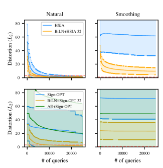
(a)

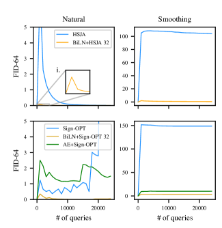
(b)

Figure 4: Results across attacks for ImageNet dataset, corresponding to a) distortion against query usage (dotted red line denotes the value of $\epsilon$, shaded areas mark standard deviation), and b) FID-64 trajectory against the same query usage.

ImageNet case study ($L_{2}$).

We attack ImageNet in the $L_{2}$-norm setting to compare against the certified smoothing technique proposed by Cohen et al. (2019). The label output comes from a smooth classifier, approximated by many rounds of Monte Carlo search, which uses the regular model regularized by Gaussian noise. Notably the smoothing occurs at inference, so there is no increase in the number of training points. The distortion results of these attacks are shown in Figure 4a. Dimension reduction has a larger impact when coupled with the large ImageNet resolution. Particularly the BiLN+HSJA (orange line, top row) and BiLN+Sign-OPT (orange line, bottom row) attacks profit the most. At 8k queries, success rate increases 1.4x and 2.1x for HSJA and Sign-OPT, respectively. This is due to 1) the AE only providing a crude approximation of the ImageNet manifold, by only having access to the test set, and 2) BiLN allowing to search closer to the original sample, since it is a deterministic function independent of the adversary’s knowledge.

The FID scores in Figure 4b paint a more comprehensive picture. BiLN variants (orange lines) produce adversarial examples closer to the manifold than either regular (blue) or AE (greeN) variants, highlighted with HSJA+BiLN in Inset 4b.i. We interpret this as follows: BiLN variants on HSJA and Sign-OPT leverage reduced dimensionality to increase the manifold-gradient mutual information, and 1) produce a smoother noise distribution, resulting in more spatially correlated distortion, which as a result 2) produces adversarial examples closer to the manifold. Another key observation is the fluctuation of LID score towards the end of Sign-OPT and AE+Sign-OPT, which are not present for HSJA (first column of Figure 4b). Notably there is no direct signal of manifold distance in the experiments, so the adversary relies on implicit manifold distance feedback from the model, which can be inaccurate.

D.2 Attacking without gradient estimate

We perform additional experiments with an attack that does not perform an explicit gradient estimate.

RayS.

Chen & Gu (2020) propose an alternative hard-label attack method which is to search for the minimum decision boundary radius $r$ from a sample $\mathbf{x}_{0}$, along a ray direction $\boldsymbol{\theta}$. Instead of searching over $\mathbb{R}^{d}$ to minimize $g(\boldsymbol{\theta})$, Chen et al. propose to perform ray search over directions $\boldsymbol{\theta}\in\{-1,1\}^{d}$, resulting in $2^{d}$ maximum possible directions. This reduction of the search resolution enables SotA query efficiency in the $L_{\infty}$ setting with proof of convergence. The search resolution is further reduced by the hierarchical variant of RayS, which performs on-the-fly upscaling of image super-pixels.

The intuition behind RayS attack is to perform a discrete search in at most $2^{d}$ directions. Chen et al. also perform a hierarchical search over progressively larger super-pixels of the image. This has the effect of already upscaling on-the-fly (Chen & Gu, 2020). RayS has the unique behavior of performing a discrete search for the decision boundary, rather than an explicit gradient estimate. To achieve an appropriate reduced-dimension version of RayS, we modify the calculation of $s$ in Algorithm 3 of Chen & Gu (2020), which either speeds up upscaling by a factor $a$ (i.e., $s=s+a$), or extends the search through a specific block index by a factor $b$ (increase block level at $k=2^{s}b$ instead of $k=2^{s}$).

Results.

The result of attacking CIFAR-10 with RayS is shown in Figure 5. The BiLN variants of RayS each have minimal effect on overall query efficiency (Insets 5a.i and 5a.ii). This is a result of RayS not relying on explicit gradient estimation. When comparing the FID-64 score, the dimension-reduced variants of RayS do not have a large variation between them (Inset 5b.i), a side-effect of the adaptive super-pixel search, which can automatically scale the super-pixel size as the search progresses.

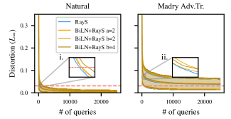
(a)

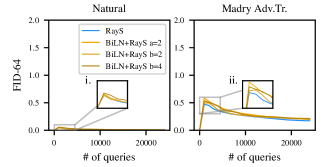
(b)

Figure 5: Results for RayS on the CIFAR-10 dataset, corresponding to a) distortion against query usage (dotted red line denotes the value of $\epsilon$, shaded areas mark standard deviation), and b) FID-64 trajectory against the same query usage.

D.3 Success Rate Plots

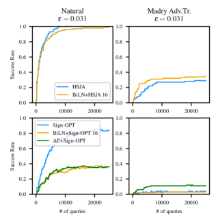
Figure 6: Query vs. success rate plots corresponding to each attack variant in the main text on CIFAR-10 .

In Figure 6 we provide query vs. success rate to accompany the results in the main text.

D.4 Tabular results - CIFAR-10

In Table 2 we provide tabular comparison at certain query intervals between regular and robust models for CIFAR-10.

	CIFAR-10 ($\epsilon=0.031$)				Madry Adv.Tr. ($\epsilon=0.031$)
	# Queries	Avg. $L_{\infty}$	SR	FID-64	# Queries	Avg. $L_{\infty}$	SR	FID-64
RayS	4,000	0.01	98.0	0.02	4,000	0.05	33.0	0.36
	8,000	0.01	100.0	0.01	8,000	0.04	36.0	0.28
	14,000	0.01	100.0	0.01	14,000	0.04	39.0	0.23
BiLN+RayS a=2	4,000	0.01	99.0	0.02	4,000	0.05	32.0	0.44
	8,000	0.01	100.0	0.01	8,000	0.05	35.0	0.33
	14,000	0.01	100.0	0.01	14,000	0.04	36.0	0.25
BiLN+RayS b=2	4,000	0.01	100.0	0.02	4,000	0.05	33.0	0.37
	8,000	0.01	100.0	0.01	8,000	0.04	37.0	0.29
	14,000	0.01	100.0	0.01	14,000	0.04	39.0	0.24
BiLN+RayS b=4	4,000	0.01	93.0	0.03	4,000	0.05	32.0	0.44
	8,000	0.01	100.0	0.02	8,000	0.05	35.0	0.33
	14,000	0.01	100.0	0.01	14,000	0.04	38.0	0.25
HSJA	4,000	0.01	88.0	0.06	4,000	0.09	15.0	3.57
	8,000	0.01	100.0	0.02	8,000	0.08	26.0	2.41
	14,000	0.01	100.0	0.01	14,000	0.06	27.0	1.69
BiLN+HSJA 16	4,000	0.02	82.0	0.03	4,000	0.07	25.0	0.68
	8,000	0.01	94.0	0.01	8,000	0.06	31.0	0.47
	14,000	0.01	97.0	0.01	14,000	0.05	32.0	0.37
Sign-OPT	4,000	0.06	52.0	0.70	4,000	0.33	2.0	2.28
	8,000	0.04	71.0	0.89	8,000	0.30	3.0	1.04
	14,000	0.02	79.0	0.00	14,000	0.28	3.0	0.59
BiLN+Sign-OPT 16	4,000	0.09	21.0	0.01	4,000	0.37	2.0	0.08
	8,000	0.06	29.0	0.00	8,000	0.35	3.0	0.04
	14,000	0.06	36.0	0.00	14,000	0.33	3.0	0.04
AE+Sign-OPT	4,000	0.09	20.0	0.01	4,000	0.20	8.0	0.01
	8,000	0.07	31.0	0.00	8,000	0.17	11.0	0.21
	14,000	0.06	35.0	0.00	14,000	0.15	11.0	0.21

Table 2: Comparison at certain query intervals between regular and robust models on CIFAR-10.

D.5 Visual results - CIFAR-10

We provide visual qualitative results for each attack on CIFAR-10 in Figure 7.

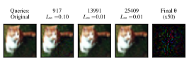
(a) Sign-OPT on CIFAR10

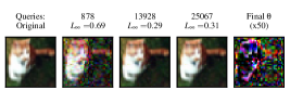
(b) Sign-OPT on CIFAR10 (Madry Adv. Tr.)

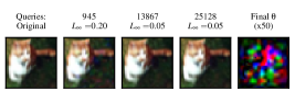
(c) BiLN Sign-OPT on CIFAR10

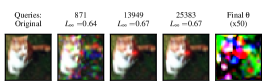
(d) BiLN Sign-OPT on CIFAR10 (Madry Adv. Tr.)

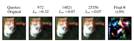
(e) AE Sign-OPT on CIFAR10

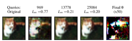
(f) AE Sign-OPT on CIFAR10 (Madry Adv. Tr.)

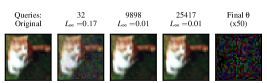
(g) HSJA on CIFAR10

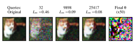
(h) HSJA on CIFAR10 (Madry Adv. Tr.)

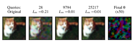
(i) BiLN HSJA on CIFAR10

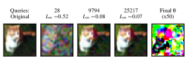
(j) BiLN HSJA on CIFAR10 (Madry Adv. Tr.)

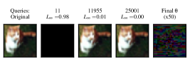
(k) RayS on CIFAR10

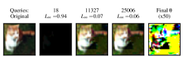
(l) RayS on CIFAR10 (Madry Adv. Tr.)

Figure 7: Visual selection of attack trajectories on CIFAR-10.

References

- Amsaleg et al. (2017) Amsaleg, L., Bailey, J., Barbe, D., Erfani, S., Houle, M. E., Nguyen, V., and Radovanović, M. The vulnerability of learning to adversarial perturbation increases with intrinsic dimensionality. In 2017 IEEE Workshop on Information Forensics and Security (WIFS), pp. 1–6, December 2017. 10.1109/WIFS.2017.8267651.
- Beaudry & Renner (2012) Beaudry, N. J. and Renner, R. An intuitive proof of the data processing inequality. arXiv:1107.0740 [quant-ph], September 2012. URL http://arxiv.org/abs/1107.0740. arXiv: 1107.0740.
- Brendel et al. (2017) Brendel, W., Rauber, J., and Bethge, M. Decision-Based Adversarial Attacks: Reliable Attacks Against Black-Box Machine Learning Models. arXiv:1712.04248 [cs, stat], December 2017. URL http://arxiv.org/abs/1712.04248. arXiv: 1712.04248.
- Carlini & Wagner (2016) Carlini, N. and Wagner, D. Towards Evaluating the Robustness of Neural Networks. In Security and Privacy (SP), pp. 582–597, 2016. ISBN 978-1-5090-5533-3. 10.1109/SP.2017.49. arXiv: 1608.04644 ISSN: 10816011.
- Carlini & Wagner (2017) Carlini, N. and Wagner, D. Adversarial Examples Are Not Easily Detected: Bypassing Ten Detection Methods. In Proceedings of the 10th ACM Workshop on Artificial Intelligence and Security - AISec ’17, pp. 3–14, Dallas, Texas, USA, 2017. ACM Press. ISBN 978-1-4503-5202-4. 10.1145/3128572.3140444. URL http://dl.acm.org/citation.cfm?doid=3128572.3140444.
- Carlini et al. (2019) Carlini, N., Athalye, A., Papernot, N., Brendel, W., Rauber, J., Tsipras, D., Goodfellow, I., Madry, A., and Kurakin, A. On Evaluating Adversarial Robustness. arXiv:1902.06705 [cs, stat], February 2019. URL http://arxiv.org/abs/1902.06705. arXiv: 1902.06705.
- Chen & Gu (2020) Chen, J. and Gu, Q. RayS: A Ray Searching Method for Hard-label Adversarial Attack. arXiv:2006.12792 [cs, stat], June 2020. URL http://arxiv.org/abs/2006.12792. arXiv: 2006.12792.
- Chen et al. (2019) Chen, J., Jordan, M. I., and Wainwright, M. J. HopSkipJumpAttack: A Query-Efficient Decision-Based Attack. arXiv:1904.02144 [cs, math, stat], April 2019. URL http://arxiv.org/abs/1904.02144. arXiv: 1904.02144.
- Chen et al. (2017) Chen, P.-Y., Zhang, H., Sharma, Y., Yi, J., and Hsieh, C.-J. ZOO: Zeroth order optimization based black-box attacks to deep neural networks without training substitute models. In ACM Workshop on Artificial Intelligence and Security, pp. 15–26, 2017.
- Cheng et al. (2019) Cheng, M., Le, T., Chen, P.-Y., Yi, J., Zhang, H., and Hsieh, C.-J. Query-efficient hard-label black-box attack: An optimization-based approach. International Conference on Learning Representations, 2019.
- Cheng et al. (2020) Cheng, M., Singh, S., Chen, P., Chen, P.-Y., Liu, S., and Hsieh, C.-J. SIGN-OPT: A QUERY-EFFICIENT HARD-LABEL ADVERSARIAL ATTACK. The International Conference on Learning Representations (ICLR), pp. 16, 2020. URL https://openreview.net/forum?id=SklTQCNtvS.
- Cohen et al. (2019) Cohen, J. M., Rosenfeld, E., and Kolter, J. Z. Certified Adversarial Robustness via Randomized Smoothing. arXiv:1902.02918 [cs, stat], February 2019. URL http://arxiv.org/abs/1902.02918. arXiv: 1902.02918.
- Cover & Thomas (2006) Cover, T. M. and Thomas, J. A. Elements of Information Theory. Wiley-Interscience. John Wiley & Sons, 2nd edition, 2006.
- Engstrom et al. (2019) Engstrom, L., Ilyas, A., Santurkar, S., Tsipras, D., Tran, B., and Madry, A. Learning Perceptually-Aligned Representations via Adversarial Robustness. arXiv:1906.00945 [cs, stat], June 2019. URL http://arxiv.org/abs/1906.00945. arXiv: 1906.00945.
- Feng et al. (2020) Feng, R., Chen, J., Manohar, N., Fernandes, E., Jha, S., and Prakash, A. Query-Efficient Physical Hard-Label Attacks on Deep Learning Visual Classification. arXiv:2002.07088 [cs], February 2020. URL http://arxiv.org/abs/2002.07088. arXiv: 2002.07088.
- Fredrikson et al. (2015) Fredrikson, M., Jha, S., and Ristenpart, T. Model Inversion Attacks that Exploit Confidence Information and Basic Countermeasures. Proceedings of the 22nd ACM SIGSAC Conference on Computer and Communications Security - CCS ’15, pp. 1322–1333, 2015. ISSN 15437221. 10.1145/2810103.2813677. URL http://dl.acm.org/citation.cfm?doid=2810103.2813677. ISBN: 9781450338325.
- Gilmer et al. (2018) Gilmer, J., Metz, L., Faghri, F., Schoenholz, S. S., Raghu, M., Wattenberg, M., and Goodfellow, I. The Relationship Between High-Dimensional Geometry and Adversarial Examples. arXiv:1801.02774 [cs], September 2018. URL http://arxiv.org/abs/1801.02774. arXiv: 1801.02774.
- Goodfellow et al. (2014) Goodfellow, I. J., Shlens, J., and Szegedy, C. Explaining and Harnessing Adversarial Examples. 2014. ISSN 0012-7183. URL http://arxiv.org/abs/1412.6572. arXiv: 1412.6572 ISBN: 1412.6572.
- Heusel et al. (2018) Heusel, M., Ramsauer, H., Unterthiner, T., Nessler, B., and Hochreiter, S. GANs Trained by a Two Time-Scale Update Rule Converge to a Local Nash Equilibrium. arXiv:1706.08500 [cs, stat], January 2018. URL http://arxiv.org/abs/1706.08500. arXiv: 1706.08500.
- Ilyas et al. (2018) Ilyas, A., Engstrom, L., Athalye, A., and Lin, J. Black-box Adversarial Attacks with Limited Queries and Information. arXiv:1804.08598 [cs, stat], July 2018. URL http://arxiv.org/abs/1804.08598. arXiv: 1804.08598.
- Jalal et al. (2019) Jalal, A., Ilyas, A., Daskalakis, C., and Dimakis, A. G. The Robust Manifold Defense: Adversarial Training using Generative Models. arXiv:1712.09196 [cs, stat], July 2019. URL http://arxiv.org/abs/1712.09196. arXiv: 1712.09196.
- Krizhevsky (2009) Krizhevsky, A. Learning Multiple Layers of Features from Tiny Images. pp. 60, 2009.
- Liu et al. (2020) Liu, S., Chen, P.-Y., Kailkhura, B., Zhang, G., Hero, A., and Varshney, P. K. A Primer on Zeroth-Order Optimization in Signal Processing and Machine Learning. arXiv:2006.06224 [cs, eess, stat], June 2020. URL http://arxiv.org/abs/2006.06224. arXiv: 2006.06224.
- Ma et al. (2018) Ma, X., Li, B., Wang, Y., Erfani, S. M., Wijewickrema, S., Schoenebeck, G., Song, D., Houle, M. E., and Bailey, J. Characterizing Adversarial Subspaces Using Local Intrinsic Dimensionality. arXiv:1801.02613 [cs], March 2018. URL http://arxiv.org/abs/1801.02613. arXiv: 1801.02613.
- Madry et al. (2017) Madry, A., Makelov, A., Schmidt, L., Tsipras, D., and Vladu, A. Towards Deep Learning Models Resistant to Adversarial Attacks. arXiv:1706.06083 [cs, stat], June 2017. URL http://arxiv.org/abs/1706.06083. arXiv: 1706.06083.
- Moosavi-Dezfooli et al. (2015) Moosavi-Dezfooli, S.-M., Fawzi, A., and Frossard, P. DeepFool: a simple and accurate method to fool deep neural networks. 2015. ISSN 10636919. 10.1109/CVPR.2016.282. URL http://arxiv.org/abs/1511.04599. arXiv: 1511.04599 ISBN: 9781467388511.
- Nesterov & Spokoiny (2017) Nesterov, Y. and Spokoiny, V. Random Gradient-Free Minimization of Convex Functions. Foundations of Computational Mathematics, 17(2):527–566, April 2017. ISSN 1615-3375, 1615-3383. 10.1007/s10208-015-9296-2. URL http://link.springer.com/10.1007/s10208-015-9296-2.
- Papernot et al. (2016) Papernot, N., Mcdaniel, P., Jha, S., Fredrikson, M., Celik, Z. B., and Swami, A. The limitations of deep learning in adversarial settings. Proceedings - 2016 IEEE European Symposium on Security and Privacy, EURO S and P 2016, pp. 372–387, 2016. 10.1109/EuroSP.2016.36. URL http://arxiv.org/abs/1511.07528. arXiv: 1511.07528 ISBN: 9781509017515.
- Russakovsky et al. (2015) Russakovsky, O., Deng, J., Su, H., Krause, J., Satheesh, S., Ma, S., Huang, Z., Karpathy, A., Khosla, A., Bernstein, M., Berg, A. C., and Fei-Fei, L. ImageNet Large Scale Visual Recognition Challenge. International Journal of Computer Vision (IJCV), 115(3):211–252, 2015. 10.1007/s11263-015-0816-y.
- Samangouei et al. (2018) Samangouei, P., Kabkab, M., and Chellappa, R. Defense-gan: Protecting classifiers against adversarial attacks using generative models. In International Conference on Learning Representations, 2018.
- Santurkar et al. (2019) Santurkar, S., Tsipras, D., Tran, B., Ilyas, A., Engstrom, L., and Madry, A. Image Synthesis with a Single (Robust) Classifier. arXiv:1906.09453 [cs, stat], June 2019. URL http://arxiv.org/abs/1906.09453. arXiv: 1906.09453.
- Schmidt et al. (2018) Schmidt, L., Santurkar, S., Tsipras, D., Talwar, K., and Madry, A. Adversarially Robust Generalization Requires More Data. arXiv:1804.11285 [cs, stat], May 2018. URL http://arxiv.org/abs/1804.11285. arXiv: 1804.11285.
- Stutz et al. (2019) Stutz, D., Hein, M., and Schiele, B. Disentangling adversarial robustness and generalization. In The IEEE Conference on Computer Vision and Pattern Recognition (CVPR), June 2019.
- Szegedy et al. (2013) Szegedy, C., Zaremba, W., Sutskever, I., Bruna, J., Erhan, D., Goodfellow, I., and Fergus, R. Intriguing properties of neural networks. pp. 1–10, 2013. ISSN 15499618. 10.1021/ct2009208. URL http://arxiv.org/abs/1312.6199. arXiv: 1312.6199 ISBN: 1549-9618.
- Szegedy et al. (2016) Szegedy, C., Vanhoucke, V., Ioffe, S., Shlens, J., and Wojna, Z. Rethinking the inception architecture for computer vision. In Proceedings of the IEEE conference on computer vision and pattern recognition, pp. 2818–2826, 2016.
- Tanay & Griffin (2016) Tanay, T. and Griffin, L. A Boundary Tilting Persepective on the Phenomenon of Adversarial Examples. arXiv:1608.07690 [cs, stat], August 2016. URL http://arxiv.org/abs/1608.07690. arXiv: 1608.07690.
- Tramer et al. (2020) Tramer, F., Carlini, N., Brendel, W., and Madry, A. On Adaptive Attacks to Adversarial Example Defenses. arXiv:2002.08347 [cs, stat], February 2020. URL http://arxiv.org/abs/2002.08347. arXiv: 2002.08347.
- Tramèr et al. (2016) Tramèr, F., Zhang, F., Epfl, F. E., Juels, A., Reiter, M. K., and Ristenpart, T. Stealing Machine Learning Models via Prediction APIs. 2016. URL https://www.usenix.org/conference/usenixsecurity16/technical-sessions/presentation/tramer. ISBN: 978-1-931971-32-4.
- Tsipras et al. (2018) Tsipras, D., Santurkar, S., Engstrom, L., Turner, A., and Madry, A. Robustness May Be at Odds with Accuracy. arXiv:1805.12152 [cs, stat], May 2018. URL http://arxiv.org/abs/1805.12152. arXiv: 1805.12152.
- Tu et al. (2019) Tu, C.-C., Ting, P., Chen, P.-Y., Liu, S., Zhang, H., Yi, J., Hsieh, C.-J., and Cheng, S.-M. AutoZOOM: Autoencoder-Based Zeroth Order Optimization Method for Attacking Black-Box Neural Networks. Proceedings of the AAAI Conference on Artificial Intelligence, 33:742–749, July 2019. ISSN 2374-3468, 2159-5399. 10.1609/aaai.v33i01.3301742. URL https://aaai.org/ojs/index.php/AAAI/article/view/3852.