Calculation of the nonlinear response functions of intra-exciton transitions in two-dimensional transition metal dichalcogenides

Abstract

In this paper, we study the third-order nonlinear optical response due to transitions between excitonic levels in two-dimensional transition metal dichalcogeniedes. To accomplish this, we use methods not applied to the description of excitons in two-dimensional materials so far and combined with a variational approach to describe the $1s$ excitonic state. The aforementioned transitions allow to probe dark states which are not revealed in absorption experiments. We present general formulas capable of describing any third-order process. The specific case of two-photon absorption in WSe₂ is studied. The case of the circular well is also studied as a benchmark of the theory.

I Introduction

Since graphene [1] was first studied the family of two-dimensional (2D) materials has been expanding, and other materials such as hexagonal-boron nitride (hBN) [2], phosphorene [3] and transition metal dichalcogeniedes (TMDs) [4], such as MoS₂, MoSe₂, WS₂ and WSe₂, have gained considerable attraction over the years. These last ones correspond to semiconducting materials with a direct band gap of about 1.5 eV [5], and are currently extensively studied due to their remarkable electronic and optical properties.

Like other 2D materials, the optical properties of TMDs are strongly dependent on their excitonic response [6]. When a material is optically excited, if the photon energy is large enough, electrons may be removed from the valence band to the conduction band. The electron promoted to the conduction band and the hole left in the valence band form a quasi-particle due to the Coulomb-like interaction between them.This particle is similar to a Hydrogen atom, and it is termed an exciton. Contrary to their 3D counterparts, where the energy spectrum is well described by a Rydberg series, excitons in 2D materials present a more complex energy landscape as a consequence of the nonlocal dielectric screening of the interaction potential between the electron and the hole [7]. Also, their reduced dimensionality leads to more tightly bound excitonic states, which are stable even at room temperature [8].

When studying the optical properties of TMDs two distinct regimes can be identified. The first one corresponds to the case where optical excitation induces transitions from the excitonic vacuum to a given state of the exciton, and is termed the excitonic interband regime. This regime is the origin of the well-known peaks in an absorption spectrum, corresponding to transitions from the excitonic vacuum to different $s-$states of the exciton [9]. In recent years, nonlinear optical effects originated from interband transitions have been the topic of many works, both experimental and theoretical. The study of nonlinearities in MoS₂ was explored in Refs. [10, 11, 12, 13], while Refs. [14, 15] studied similar effects in WS₂ and Refs. [16, 17] in WSe₂. A thorough comparison between the nonlinear response of different TMDs is presented in Ref. [18]. Studies on the effect of strain and the coupling to exciton-plasmons have also been performed [19, 20]. In Ref. [21] an analytical study of the nonlinear optical response of monolayer TMDs was presented. Due to their broken inversion symmetry TMDs are not centrosymmetric (at least when stacked in an odd number of layers), and as a consequence both even and odd orders of non linear optical processes are always permitted [22]. Moreover, these materials shown large nonlinear optical coefficients [21], increasing their potential for applications, such as optical modulators [23, 24]. The possibility of characterizing different properties of the 2D material from their nonlinear optical response has also been considered [25, 26]. The second regime one should consider when studying the optical properties of these systems is associated with transition between the excitonic energy levels themselves, and we label it as the intra-exciton regime. This type of excitation can be experimentally realized in a pump-probe setup, where first the pump laser populates the $1s$ exciton state and then the probe induces transitions from the $1s$ to the remaining bound states of the exciton. Recently, in Ref. [27], this type of procedure was implemented to characterize the linear optical response of WSe₂ in the intra-exciton regime, and probe the excitonic dark states which are not accessible from luminescence methods. Contrary to the interband regime, the nonlinear response associated with optical transitions when the ground state is already populated remains vastly unstudied. Its comprehension could unlock new degrees of freedom exploitable in nonlinear optical applications.

Our goal with this paper is to provide a theoretical framework based on the ideas presented in Refs. [28, 29, 30, 31, 32], which allows the description of third-order nonlinear optical processes in the intra-exciton regime, namely the two photon absorption (TPA) for excitons in WSe₂. Contrarily to the approach of a sum over states usually found from time-dependent perturbation theory, where different excited wave functions are needed, our approach only requires the $1s$ wave function, which can be accurately described using variational techniques [33, 34]. We then expand the perturbed wave function directly in a basis. It follows that, formally, our approach is equivalent to a sum of states computation approximating excited states by expanding in the same basis. However, the present approach is conceptully simpler. The text is organized as follows. In Sec. 2 we present the general method used to compute the nonlinear third-order optical susceptibility. This corresponds to a generalization of the approach presented in Ref. [35] where the linear response was studied. In Sec. 3 we focus on the more interesting problem of excitons in WSe₂, when the excitonic ground state is already populated and the optical excitation induces transitions between the excitonic levels. A section with our final remarks and an appendix close the paper.

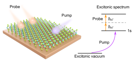
Figure 1: Schematic representation of the two photon absorption process in WSe₂ excitons when the 1$s$ excitonic state is already populated.

II Nonlinear third-order optical response

In the first part of this section we will give a detailed description of a method to compute the third-order optical susceptibility of a given system. The only requirement is that the ground-state wave function of the system is known (at least approximately). This method contrasts with the usual sum over states where both the ground state and the excited-state wave functions are needed. The presented approach is based on Refs. [28, 29, 30, 31, 32] and corresponds to an extension of what was recently used in Ref. [35] regarding the linear optical response. In the second part of the section the problem of a circular potential well will be studied as a first application of the formalism. This example will set the stage for the posterior study of two–dimensional excitons in WSe₂.

II.1 Outline of the Method

II.1.1 Third-order susceptibility

Since we will be interested in computing the third-order nonlinear response, we start by introducing the expression for the third-order optical susceptibility, as derived from perturbation theory. Throughout the work we will use atomic units unless stated otherwise. Following Ref. [36] we write the third-order susceptibility as

$$\chi_{\alpha\beta\gamma\delta}^{(3)}({\omega_{\sigma}};\omega_{1},\omega_{2},\omega_{3})=$$

$$= \frac{1}{3!}\mathcal{P}\Bigg{\{}\sum_{n,m,l\neq 0}\frac{\langle 0|\mathbf{d}_{\alpha}|n\rangle\langle n|\mathbf{d}_{\beta}|m\rangle\langle m|\mathbf{d}_{\gamma}|l\rangle\langle l|\mathbf{d}_{\delta}|0\rangle}{(E_{n0}-\omega_{\sigma})(E_{m0}-\omega_{2}-\omega_{3})(E_{l0}-\omega_{3})}$$

$$- \sum_{n,m\neq 0}\frac{\langle 0|\mathbf{d}_{\alpha}|n\rangle\langle n|\mathbf{d}_{\beta}|0\rangle\langle 0|\mathbf{d}_{\gamma}|m\rangle\langle m|\mathbf{d}_{\delta}|0\rangle}{(E_{n0}-\omega_{\sigma})(E_{m0}-\omega_{2})(E_{m0}+\omega_{1})}\Bigg{\}},$$ (1)

where, $E_{n0}=E_{n}-E_{0}$ is the energy difference between the levels $|n\rangle$ and $|0\rangle$, $\mathbf{d}$ is the dipole moment, $\{\alpha,\beta,\gamma,\delta\}$ are indexes corresponding to different spatial orientations ($x$ or $y$), $\omega_{\sigma}=\omega_{1}+\omega_{2}+\omega_{3}$, $\mathcal{P}$ is the permutation operator of the pairs $(\alpha,-\omega_{\sigma};\beta,\omega_{1};\gamma,\omega_{2};\delta,\omega_{3})$ and $|n\rangle$ corresponds to the unperturbed states of the system, with $|0\rangle$ its ground state. The direct application of Eq. (1) corresponds to the sum over states approach. Since the different sums run over all the excited states of the system, this way of calculating the optical susceptibility presents the major drawback of requiring the knowledge of all the excited-state wave functions, at least in a naive approach (obviously one can expand the unknown eigenstates in a complete basis and obtain the expansion coefficients. This latter approach can be seen as an alternative to the method developed in the Appendix A). Although in simple systems the exact wave functions may be trivially known, in more complex ones they may be elusive (this is precisely the case of excitons in 2D materials to be discussed ahead).

In order to avoid the usual sum over states method we follow the ideas of Refs. [28, 29, 30, 31, 32]. Doing so, we write the time-dependent Schrödinger equation

$$\left[H_{0}+\mathbf{d}\cdot\boldsymbol{\mathcal{E}}(t)\right]|\psi(t)\rangle=i\frac{\partial}{\partial t}|\psi(t)\rangle.$$ (2)

where $H_{0}$ corresponds to the unperturbed Hamiltonian of a given system (this may contain a kinetic and a potential term), $\mathbf{d}\cdot\boldsymbol{\mathcal{E}}(t)$ describes the interaction of the system with an external time-dependent harmonic electric field $\boldsymbol{\mathcal{E}}(t)$ in the dipole approximation, and $|\psi(t)\rangle$ is the state vector of the system in the presence of the external electric field. Next, we expand $|\psi(t)\rangle$ in powers of $\mathcal{E}$ as

$$|\psi\rangle =|0\rangle e^{-iE_{0}t}+\mathcal{E}_{\alpha}|\psi_{\alpha}\rangle e^{-i(E_{0}-\omega_{a})t}$$

$$+\mathcal{E}_{\alpha}\mathcal{E}_{\beta}|\xi_{\alpha\beta}\rangle e^{-i(E_{0}-\omega_{a}-\omega_{b})t}+...$$ (3)

where $\boldsymbol{\mathcal{E}}_{\alpha}e^{i\omega_{a}t}$ refers to an harmonic electric field applied along the $\alpha$ direction (either $x$ or $y$) with frequency $\omega_{a}$, $E_{0}$ is the energy of the unperturbed ground state of the system and $|\psi_{\alpha}\rangle$ and $|\xi_{\alpha\beta}\rangle$ are yet to be determined. Inserting this in the time-dependent Schrödinger equation and grouping equivalent terms in $\mathcal{E}$, up to second order in the electric field, we find the following three equations

$$0 =\left(H_{0}-E_{0}\right)|0\rangle$$ (4)

$$0 =\left(H_{0}-E_{0}+\omega_{a}\right)|\psi_{\alpha}\rangle+\mathbf{d}_{\alpha}|0\rangle$$ (5)

$$0 =\left(H_{0}-E_{0}+\omega_{a}+\omega_{b}\right)|\xi_{\alpha\beta}(\omega_{a},\omega_{b})\rangle+\mathbf{d}_{\beta}|\psi_{\alpha}(\omega_{a})\rangle.$$ (6)

The first one simply states the eigenvalue relation for the ground state of the system in the absence of the external electric field. The second and third ones define the $|\psi_{\alpha}\rangle$ and $|\xi_{\alpha\beta}\rangle$, respectively. Expanding these two states in the basis of the eigenstates of $H_{0}$ one easily arrives at

$$|\psi_{\alpha}(\omega_{a})\rangle =-\sum_{n\neq 0}\frac{\langle n|\mathbf{d}_{\alpha}|0\rangle}{E_{n}-E_{0}+\omega_{a}}|n\rangle,$$ (7)

$$|\xi_{\alpha\beta}(\omega_{a},\omega_{b})\rangle =-\sum_{n\neq 0}\frac{\langle n|\mathbf{d}_{\beta}|\psi_{\alpha}(\omega_{a})\rangle}{E_{n}-E_{0}+\omega_{a}+\omega_{b}}|n\rangle,$$ (8)

where we assumed $\langle 0|\psi_{\alpha}\rangle=0$ and $\langle 0|\xi_{\alpha\beta}\rangle=0$. The first requirement corresponds to choosing a coordinate system placing $\langle 0|\mathbf{d}|0\rangle$ at the origin, which is always possible. The second assumption will be discussed further ahead. Now we note that with the introduction of $|\psi_{\alpha}\rangle$ and $|\xi_{\alpha\beta}\rangle$ we are able to rewrite Eq. (1) without the sums over the excited states, hence

$$\chi_{\alpha\beta\gamma\delta}^{(3)} =\frac{1}{3!}\mathcal{P}\Big{\{}-\langle\psi_{\alpha}\left(-\omega_{\sigma}^{*}\right)|\mathbf{d}_{\beta}|\xi_{\delta\gamma}(-\omega_{3},-\omega_{2})\rangle$$

$$+\langle 0|\mathbf{d}_{\alpha}|\psi_{\beta}(-\omega_{\sigma})\rangle\langle\psi_{\gamma}\left(-\omega_{2}^{*}\right)|\psi_{\delta}(\omega_{1})\rangle\Big{\}}.$$ (9)

Thus, using the ideas of Ref. [28, 29, 30, 31, 32], we shifted the problem away from the sum over states, to the determination of two new state vectors $|\psi_{\alpha}\rangle$ and $|\xi_{\alpha\beta}\rangle$. After being determined, these state vectors allow us to access the third-order susceptibility through the computation of only three matrix elements. Note that we are considering the possibility of the frequencies to be complex valued. We do so in order to obtain both the real and imaginary parts of $\chi^{(3)}$ . This is achieved by shifting the energies by a small imaginary part, that is $\omega\rightarrow\omega+i\delta$.

II.1.2 Computing the new state vectors

Now that an alternative path to the sum over states was found, we are left with the task of determining $|\psi_{\alpha}\rangle$ and $|\xi_{\alpha\beta}\rangle$. Computing these quantities using Eq. (7) and (8) would reverse our progress, and leave us again with a problem requiring the calculation of a sum over states. To continue with the calculations, we follow Ref. [28] and introduce the functionals

$$\mathcal{J} =\langle\psi_{\alpha}(\omega)|H_{0}-E_{0}+\omega|\psi_{\alpha}(\omega)\rangle$$

$$+\langle\psi_{\alpha}(\omega)|\mathbf{d}_{\alpha}|0\rangle+\langle 0|\mathbf{d}_{\alpha}|\psi_{\alpha}(\omega)\rangle,$$ (10)

and

$$\mathcal{K} =\langle\xi_{\alpha\beta}(\omega_{a},\omega_{b})|\left(H_{0}-E_{0}+\omega_{a}+\omega_{b}\right)|\xi_{\alpha\beta}(\omega_{a},\omega_{b})\rangle$$

$$+\langle\xi_{\alpha\beta}(\omega_{a},\omega_{b})|\mathbf{d}_{\beta}|\psi_{\alpha}(\omega_{a})\rangle+\langle\psi_{\alpha}(\omega_{a})|\mathbf{d}_{\beta}|\xi_{\alpha\beta}(\omega_{a},\omega_{b})\rangle.$$ (11)

Minimizing $\mathcal{J}$ with respect to $|\psi_{\alpha}\rangle$ and $\mathcal{K}$ with respect to $|\xi_{\alpha\beta}\rangle$ allows us to explicitly compute these new state vectors. . Moreover, we note that the minimization of these functionals is equivalent to directly solving Eq. (5) and (6), where $|\psi_{\alpha}\rangle$ and $|\xi_{\alpha\beta}\rangle$ were first introduced.

Since we will be interested in 2D systems, the first step in our procedure is to confine our system within a disk of radius $R$. If the problem we are interested in is not naturally bounded, we can first force it to be defined inside a disk of finite radius, and later chose $R\gg 1$ and check the convergence of the results by varying $R$. This procedure is always possible as long as the wave functions vanish for a large enough distance away from the origin. After this is done we can expand $|\psi_{\alpha}\rangle$ and $|\xi_{\alpha\beta}\rangle$ in a Fourier-Bessel series with a normalised radial basis

$$j_{ln}(r)=\frac{\sqrt{2}J_{l}\left(\frac{z_{ln}r}{R}\right)}{J_{l+1}(z_{ln})R},$$ (12)

where $J_{l}(z)$ is the Bessel function of the first kind of $l$’th order, $z_{ln}$ corresponds to the $n$’th zero of $J_{l}(z)$, and $R$ is the radius of the disk where the problem is defined. In terms of this basis,

$$\psi_{\alpha}(\omega;\mathbf{r}) =\frac{1}{\sqrt{2\pi}}\sum_{n=1}^{N}\sum_{l=\pm 1}c_{ln}^{\alpha}(\omega)j_{ln}(r)e^{il\theta}$$

$$=\frac{1}{\sqrt{2\pi}}\sum_{n=1}^{N}\left[c_{+,n}^{\alpha}(\omega)e^{i\theta}-c_{-,n}^{\alpha}(\omega)e^{-i\theta}\right]j_{1n}(r),$$ (13)

and

$$\xi_{\alpha\beta}(\omega_{a},\omega_{b};\mathbf{r})=\frac{1}{\sqrt{2\pi}}\sum_{n=1}^{N}\sum_{l=-\infty}^{\infty}\zeta_{ln}^{\alpha\beta}(\omega_{a},\omega_{b})j_{ln}(r)e^{il\theta},$$ (14)

where $N$ is the number of functions in the radial basis, $c_{ln}^{\alpha}$ and $\zeta_{ln}^{\alpha\beta}$ are the expansion coefficients, and $(r,\theta)$ are polar coordinates. Although we choose to work with a Fourier-Bessel basis, other options could have been used, e.g. orthogonal polynomials or Sturmian functions. Now, we insert these expressions in the definitions of $\mathcal{J}$ and $\mathcal{K}$ and minimize each functional with respect to the $c_{ln}^{\alpha}$ and $\zeta_{ln}^{\alpha\beta}$ respectively. Doing so we arrive at two linear system of equations whose solutions define the expansion coefficients. In Appendix A we give the detailed description of the necessary steps to obtain the linear system of equations, which is numerically well behaved and can be easily solved. Also discussed in the Appendix is the implication of the condition $\langle 0|\xi_{\alpha\beta}\rangle=0$, which imposes a restriction on the coefficient $\zeta_{01}^{\alpha\beta}$, requiring special care when dealing with the term $l=0$ in the functional $\mathcal{K}$.

II.2 The case of the circular well

Up to this point have introduced the third-order optical susceptibility, and presented a way of computing it without a sum over states. To do this, two new state vectors, $|\psi_{\alpha}\rangle$ and $|\xi_{\alpha\beta}\rangle$, were introduced. The necessary steps to find both $|\psi_{\alpha}\rangle$ and $|\xi_{\alpha\beta}\rangle$ were already briefly discussed and their detailed description is given in Appendix A. Now, as a first application of the ideas presented so far, we will study the problem of a circular well. This studywill allow for a concrete application of the general expressions previously derived, as well as gaining some intuition that will prove helpful when the excitonic problem is studied ahead.

Consider a particle with mass $\mu$ trapped inside a circular well of radius $R$. The Hamiltonian of such a system reads

$$H=-\frac{1}{2\mu}\nabla^{2},\quad 0\leq r/R<1.$$ (15)

The eigenstates are given by

$$\psi_{nm}(r,\theta)=\frac{1}{\sqrt{2\pi}}j_{mn}(r)e^{im\theta}.$$ (16)

Following common practice, we label $n$ as the principal quantum number and $m$ as the angular quantum number. The energy spectrum reads

$$E_{nm}=\frac{1}{2\mu}\left(\frac{z_{mn}}{R}\right)^{2}.$$ (17)

The ground-state wave function is $\psi_{\rm GS}(r)=j_{01}(r)/\sqrt{2\pi}$.

There are many nonlinear third-order optical processes [37]. To be definitive, let us now focus on a specific third-order nonlinear optical process. We will be interested in computing the $xxxx$ component of the two photon absorption (TPA) third-order susceptibility $\chi_{xxxx}^{{\rm TPA}}(\omega)=\chi_{xxxx}^{(3)}(-\omega;\omega,-\omega,\omega)$. Using Eq. (9), we write

$$\chi_{xxxx}^{{\rm TPA}} =\frac{1}{3!}\mathcal{P}\Big{\{}-\langle\psi_{x}\left(-\omega^{*}\right)|\mathbf{d}_{x}|\xi_{xx}(-\omega,\omega)\rangle$$

$$+\langle 0|\mathbf{d}_{x}|\psi_{x}(-\omega)\rangle\langle\psi_{x}\left(-\omega^{*}\right)|\psi_{x}(\omega)\rangle\Big{\}}.$$ (18)

To obtain the TPA spectrum we need only compute $\psi_{x}$ and $\xi_{xx}$ using the procedure discussed previously, and then evaluate three matrix elements. A detailed description of this is given in Appendix B. The fact that the potential vanishes inside the disk of radius $R$ makes this a simple application of the ideas so far introduced. Considering $\mu=1$ and $R=1$, using $N=5$ basis functions, and accounting for all the necessary permutations in Eq. (18), we obtain the results depicted in Fig. 2. This value of $N$ already allows the results to converge; increasing it produces no change in the TPA spectrum. In order to obtain the real and imaginary parts of $\chi_{xxxx}^{{\rm TPA}}(\omega)$ we introduced a small imaginary shift in the frequency $\omega$, i.e. $\omega\rightarrow\omega+i\delta$. The resonances that appear in Fig. 2 have two distinct origins the ones marked with the orange lines correspond to transitions from the ground state (which we call the 1$s$ state) to other $s-$states (where the angular quantum number is $m=0$) with the absorption of two photons; the ones marked with the green lines are associated with transitions from the ground state to $d-$states ($m=2$), due to the absorption of two photons. As the principal quantum number of the final state increases, the oscillator strength of the transition decreases and the resonances become less pronounced. One of the main advantages of studying the circular well lies in its parabolic energy spectrum (see Eq. (17)), since the energy levels are significantly separated, allowing for an effortless identification of the relevant optical transitions.

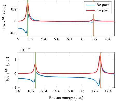
Figure 2: Plot of the two-photon absorption (TPA) third-order susceptibility as a function of the photon energy for a particle with mass $\mu=1$ in a circular well of radius $R=1$. Both quantities are presented in atomic units (a.u.). The resonances marked with the orange lines correspond to transitions from the ground state (1$s$) to the states 2$s$ and $3s$ with the absorption of two photons. The resonances marked with the green lines are associated with the transitions $1s\rightarrow 1d$ and $1s\rightarrow 2d$. As the principal quantum number of the final state increases, the oscillator strength of the resonance decreases. In order to obtain the real and imaginary parts we introduced a small shift in the frequency $\omega$, that is, $\omega\rightarrow\omega+i\delta$ with $\delta=0.02$ a.u.. $N=5$ basis functions were used.

III Two-photon absorption for excitons in ${\rm WS}$${\rm e}_{2}$

In the previous section we presented a method to compute the third-order optical susceptibility of a system without performing a sum over states. Afterwards we explored the problem of a circular disk as a first application of the formalism. Now, in the current section, we will discuss the more interesting topic of 2D excitons in WSe₂. More accurately, we will study the third-order optical response associated with transitions from the ground state ($1s$) to excited states of the 2D exciton. This problem is the natural extension of the work done in [35] and the computed physical quantity can be measured experimentally in a pump-probe experiment.

The Hamiltonian that describes the excitonic problem reads

$$H_{0}=-\frac{1}{2\mu}\nabla^{2}+V_{{\rm RK}}(r),$$ (19)

where $\mu$ is the reduced mass of the electron–hole pair, $\nabla^{2}$ is the 2D Laplacian and $V_{{\rm RK}}(r)$ is the Rytova-Keldysh potential [38, 39]

$$V_{{\rm RK}}=-\frac{\pi}{2r_{0}}\left[\mathbf{H}_{0}\left(\frac{\kappa r}{r_{0}}\right)-Y_{0}\left(\frac{\kappa r}{r_{0}}\right)\right],$$ (20)

where $\kappa$ is the mean dielectric constant of the media above and below the TMD, $r_{0}$ is an intrinsic parameter of the 2D material which can be interpreted as an in-plane screening length and is related to the effective thickness of the material; $\mathbf{H}_{0}$ and $Y_{0}$ are the Struve function and the Bessel function of the second kind, both of order 0, respectively. This potential is the solution of the Poisson equation for a charge embedded in a thin film. For large distances the Rytova-Keldysh presents a Coulomb$-1/\kappa r$ tail, but diverges logarithmically near the origin.

While in the previous section we showed the usefulness of our approach when we computed $\chi_{xxxx}^{{\rm TPA}}(\omega)$ for the circular well without evaluating a sum over states, the true potential of the method is clearer when it is applied to the excitonic problem. Contrary to the circular well, or even the Hydrogen atom, the 2D excitonic problem does not offer a simple analytical solution. In fact, computing the wave functions of the different excitonic states is an involved problem, where the wave functions are only known either numerically or semi-analytically (where the wave functions can be computed analytically up to a set of numerical coefficients). In the present approach, perturbed wave functions are computed directly by expanding in a basis without the intermediate step of finding excited states. We have shown that in order to apply the formalism presented in Sec. 2 only the wave function of the exciton ground state is required. Finding this wave function is a considerably simpler task, and in order to work with an analytical expression we follow a variational approach. To obtain accurate results for the optical susceptibility, it is necessary to use an appropriate ground-state wave function. It is thus imperative that our variational ansatz produces an excellent description of the exact solution. A first proposal for the variational ansatz, inspired by the 2D Hydrogen atom, could be a single exponential such as $\exp(-ar)$, where $a$ is a variational parameter. Although this already produces a good description of the exact ground-state wave function, we turn to Ref. [33], where a more sophisticated double exponential ansatz was proposed

$$\psi_{{\rm GS}}(r)=\frac{1}{\sqrt{\mathcal{N}}}\left(e^{-ar}+be^{-a\gamma r}\right),$$ (21)

with $a$, $b$ and $\gamma$ variational parameters and $\mathcal{N}$ a normalization constant. As one can observe in Fig. 3, where the exact wave function is compared with the single and double exponential ansaetze for excitons in WSe₂, Eq. (21) produces an outstanding description of the exact solution, the latter computed with a numerical shooting algorithm. As we have already noted in Sec. 2, the domain of our problem should be enclosed within a disk of finite radius. However, the excitonic problem is usually considered as an unbounded one, and the wave functions extend up to infinity, where they smoothly vanish. In practice, we find that the ground state wave function has vanished at $r=R$ to an excellent approximation and, hence, contributions from the edge are negligible.

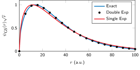
Figure 3: Comparison between the excitonic ground-state wave function obtained exactly (using a shooting algorithm), and the ones obtained with the single and double variational ansaetze. Although the single exponential approach already produces a good result, the one obtained with the double exponential is clearly superior. The values of the variational parameters were obtained from the minimization of the expected value of the Hamiltonian of Eq. (20). The values of Table 1 were used.

As in the case of the circular well, let us consider the $xxxx$ component of the TPA susceptibility associated with transitions from the 1$s$ to the excited excitonic states. Its general expression was already given in Eq. (18). To evaluate the TPA spectrum we return once more to the problem of minimizing the $\mathcal{J}$ and $\mathcal{K}$ functionals.. A difference relatively to the circular well lies in the value of $\zeta_{01}$. The orthogonality of Bessel functions on a disk implied that $\zeta_{01}=0$ for the circular well. For the excitonic problem no simple rule applies, and the value of $\zeta_{01}$ must be determined from Eq. (30).

Using the parameters given in Table 1 the TPA spectrum plotted in Fig. 4 was obtained.

$\mu$	$\kappa$	$r_{0}$	$R$	$N$
0.167	3.32	51.9	2500	150

Table 1: Parameters used to compute the TPA spectrum due to intra-excitonic transition in WSe₂. All the quantities are given in atomic units. The values of $\mu$, $\kappa$ and $r_{0}$ were taken from Ref. [27]. The value of $R$ was chosen in order to have $\psi_{{\rm GS}}(R)\approx 0$. The value of $N$ allowed the results to converge.

The value of $R$ was chosen such that $\psi_{{\rm GS}}(R)\approx 0$. A small value for the radius modifies the results due to the effect of the confinement that we introduced in the problem. A larger value for $R$ suppresses the effect of the confinement at the cost of increased convergence difficulty, as a larger $R$ requires a higher $N$. We found that $R=2500$ allows an accurate description of the excitonic problem, while keeping the method efficient. The number of functions that make up the Fourier-Bessel basis was chosen as the minimum $N$ which when increased leaves the result unchanged. The results proved to be stable with respect to small variations of both $N$ and $R$, and inspection of the different coefficients that appear in the Fourier-Bessel expansions confirmed the convergence of the results.

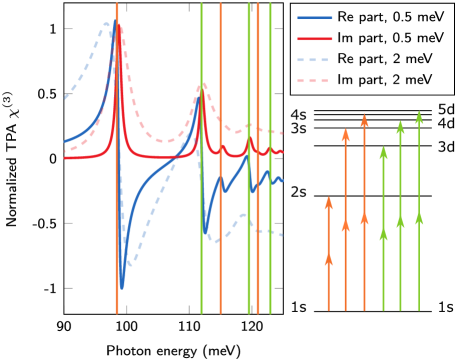
Figure 4: Real and imaginary parts of the TPA susceptibility (normalized to its maximum valued) for two different degrees of disorder (0.5 and 2 meV). The resonances correspond to transitions from the $1s$ to the $2s$, $3s$ and $4s$ states (marked in orange) and to the $3d$, $4d$ and $5d$ states (marked in green) with the absorption of two photons. The energies of these transitions were computed from the binding energies of the involved states which in turn were obtained numerically using a shooting algorithm. A diagram of the optical transitions behind the resonances is also depicted.

Looking at Fig. 4 we observe a similar result to the one found for the circular well. In order to identify the optical transitions behind each resonance we computed the energy of the different excitonic states using a shooting algorithm, and from there the energies of the transitions from the $1s$ to other states were computed. This allowed us to assert that the resonances in Fig. 4 are due to transitions from the ground state ($1s$) to the $2s$, $3s$ and $4s$ states (marked in orange) and to the $3d$, $4d$ and $5d$ states (marked in green) with the absorption of two photons. The identification of the optical transitions behind each resonance was also facilitated by the intuition gained from the study of the circular well. The real and imaginary parts of the TPA susceptibility were obtained by introducing a small imaginary part on the photon energy $\omega\rightarrow\omega+i\delta$, where the parameter $\delta$ characterizes the broadening of the excitonic level. As expected, increasing the value of $\delta$ leads to broader and less intense resonances. For large values of $\delta$ a nonphysical shift of the resonance starts to appear. This effect is the main limitation of our approach. Currently it is possible to study this kind of system with a linewidth of about 20 meV for a sample on glass [40], and for encapsulated systems at low temperatures spectral broadening as low as 2 meV can be achieved [41]. From the results depicted in Fig. 4, where the maximum broadening is 2 meV, we expect that experimental measurements of the TPA performed on encapsulated systems should be able to clearly capture the resonances originated by the $1s\rightarrow 2s$, $1s\rightarrow 3d$ and $1s\rightarrow 3s$ transitions. In order to capture more resonances it is necessary to decrease the linewidth, or change the studied material to another where the excitonic resonances are further apart (such as hBN).

In Fig. 5 we study the role of the dielectric environment on the TPA spectrum. This parameter appears in the calculation inside the Rytova-Keldysh potential. As the dielectric screening is reduced, that is $\kappa$ decreases, the excitons become more tightly bound. As a consequence, the energy difference between the ground state and the excited excitonic states increases. This behavior is reflected in Fig. 5, where we observe a blue-shift of the resonances as $\kappa$ decreases. Moreover, we also observe that the oscillators strength decreases with decreasing dielectric screening.

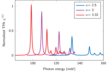
Figure 5: Comparison of the TPA spectrum for three different dielectric environments, $\kappa=3.32$, $\kappa=3$ and $\kappa=2.5$. As the dielectric constant decreases the excitons become more tightly bound, the energetic difference between the ground state and the excited states increases and the resonances are shifted to higher energies.

IV Conclusion

In this work, following the ideas of Refs. [28, 29, 30, 31, 32], we developed a method to study nonlinear third order processes involving transitions from the 1$s$ to excited excitonic states. The usual approach to this type of problem would require the knowledge of all the excited states in order to compute the different matrix elements that appear in Eq. (1). The excited states wave functions are often computed by expanding them in a given basis, e.g. Bessel-Fourier, followed by the diagonalization of the Hamiltonian. This yields the sets of coefficients that define the wave functions of the different excited states, which can then be used to evaluate the many matrix elements in the sum over states. At odds with this procedure, our approach avoids the sum over states, and requires only three wave functions: the ground state wave function, which can be described using a variational ansatz with high accuracy (see Fig. 3); and two wave functions defined by Eqs. (7) and (8) which we determined through an expansion in a Bessel-Fourier basis.

The main result of our work is the TPA spectrum which presents resonances associated with transitions from the $1s$ state to the remaining $s-$states as well as from the $1s$ to the $d-$states with the absorption of two photons. In high purity systems different resonances should be resolvable. However, in systems with a significant spectral broadening only the $1s\rightarrow 2s$ resonance should be identifiable. When the role of dielectric screening was studied, a blue shift of the resonances was observed with decreasing dielectric constant, in agreement with the increased exciton binding energy and higher energy separation between the ground state and the excited states. We focused on the case of excitons in WSe₂, but other materials may easily be explored using the method.

Although we focused primarily on the $xxxx$ component of the TPA susceptibility, we presented general formulas capable of describing any third-order process in an arbitrary system as long as its ground state wave function is know, either exactly or approximately. The study of systems where confinement plays a significant role, such as quantum dots, may also be treated with this approach.

Appendix A Computing the new state vectors

In this appendix we will give a detailed description of how to obtain the linear systems whose solution defines the state vectors $|\psi_{\alpha}\rangle$ and $|\xi_{\alpha\beta}\rangle$. Let us consider the $H_{0}$ to be the unperturbed Hamiltonian of a given system which in general can be written as

$$H_{0}=-\frac{1}{2\mu}\nabla^{2}+V(r),$$ (22)

where the first term, with $\mu$ a mass term and $\nabla^{2}$ the 2D laplacian, corresponds to the kinetic energy, and $V(r)$ corresponds to the potential energy. Here, we consider a central potential for which the ground state may be expressed as $\psi_{{\rm GS}}\left(\boldsymbol{r}\right)=R_{\rm GS}\left(r\right)/\sqrt{2\pi}$. Inserting Eqs. (13) and (22) into Eq. (10) one finds

$$\mathcal{J} =\sum_{n=1}^{N}\sum_{l=\pm}c_{ln}^{\alpha}\left(c_{ln}^{\alpha}\right)^{*}\left[\frac{1}{2\mu}\left(\frac{z_{ln}}{R}\right)^{2}-E_{0}+\omega\right]$$

$$+\sum_{n=1}^{N}\sum_{k=1}^{N}\sum_{l=\pm}c_{ln}^{\alpha}\left(c_{lk}^{\alpha}\right)^{*}\mathcal{V}_{kn}^{(l)}$$

$$+\frac{1}{2}\sum_{n=1}^{N}\sum_{l=\pm}\left[\left(\delta_{\alpha,x}-il\delta_{\alpha,y}\right)\left(c_{ln}^{\alpha}\right)^{*}\mathcal{S}_{n}^{(l)}+c.c.\right],$$ (23)

where $c.c.$ stands for complex conjugated and the following integrals where introduced

$$\mathcal{V}_{kn}^{(l)} =\int_{0}^{R}j_{lk}(r)V(r)j_{ln}(r)rdr,$$ (24)

$$\mathcal{S}_{n}^{(l)} =\int_{0}^{R}j_{ln}(r)R_{\rm GS}(r)r^{2}dr.$$ (25)

The first one corresponds to the matrix elements of the potential between different basis functions, while the second one is proportional to dipole transitions between the ground state of the unperturbed system and the functions of the basis. Furthermore, we note that $\mathcal{V}_{kn}^{(l)}$ is symmetric, that is, $\mathcal{V}_{kn}^{(l)}=\mathcal{V}_{nk}^{(l)}$. We have omitted the argument of the coefficients $c_{ln}^{\alpha}$ to simplify the notation, however one should keep in mind that these are $\omega-$dependent quantities.

Now, differentiating $\mathcal{J}$ with respect to the coefficients $\left(c_{ln}^{\alpha}\right)^{*}$, we obtain a linear system of equations whose solution determines the coefficients themselves. In matrix notation the linear system reads

$$\mathbb{M}^{(l)}(\omega)\mathbf{c}_{l}^{\alpha}(\omega) =-\frac{1}{2}\left(\delta_{\alpha,x}-il\delta_{\alpha,y}\right)\mathbf{S}^{(l)},\quad l=\pm 1$$ (26)

where

$$\left[\mathbb{M}^{(l)}(\omega)\right]_{ij}=\delta_{ij}g_{j}^{(l)}(\omega)+\mathcal{V}_{ij}^{(l)},$$ (27)

with

$$g_{j}^{(l)}(\omega)=\frac{z_{lj}^{2}}{2\mu R^{2}}-E_{0}+\omega,$$ (28)

and

$$\left[\mathbf{S}^{(l)}\right]^{{\rm T}} =\left[\mathcal{S}_{1}^{(l)},\mathcal{S}_{2}^{(l)},\ldots,\mathcal{S}_{N}^{(l)}\right],$$

$$\left[\mathbf{c}_{l}^{\alpha}(\omega)\right]^{{\rm T}} =\left[c_{l1}^{\alpha}(\omega),c_{l2}^{\alpha}(\omega),\ldots,c_{lN}^{\alpha}(\omega)\right].$$

Let us emphasize that to obtain the coefficients that define $|\psi_{\alpha}\rangle$ we need only compute the vector $\mathbf{S}^{(l)}$ and the matrix $\mathbb{M}^{(l)}$. The most expensive part of the numerical computation is the calculation of all the $\mathcal{V}_{ij}^{(l)}$. However, since $\mathcal{V}_{ij}^{(l)}$ is independent of $\omega$ this only needs to be computed once, regardless of the value of $\omega$ one wishes to use. The fact that $\mathcal{V}_{ij}^{(l)}$ is symmetric also greatly reduces the number of integrals that need to be evaluated. Finally, we point out that when $\alpha=x$ we have $c_{+,n}^{x}=-c_{-,n}^{x},$ since $\mathbb{M}^{(+)}=\mathbb{M}^{(-)}$ and $\mathbf{S}^{(+)}=-\mathbf{S}^{(-)}.$ Following the same reasoning, when dealing with the $y$ direction we have $c_{+,n}^{y}=c_{-,n}^{y}$, due to the term $il\delta_{\alpha,y}$ which changes sign when $l$ changes sign.

With the problem associated with the functional $\mathcal{J}$ taken care of, let us move on to the functional $\mathcal{K}.$ Once again we choose to work in a Fourier-Bessel basis. Now, let us recall that in the beginning, following Eq. (8), we assumed $\langle 0|\xi_{\alpha\beta}(\omega_{a},\omega_{b})\rangle=0$. In order to satisfy this, we must have

$$\sum_{n=1}^{N}\zeta_{0n}^{\alpha\beta}(\omega_{a},\omega_{b})\int_{0}^{R}j_{0n}(r)R_{{\rm GS}}(r)rdr =0,$$ (29)

where all the reaming terms in the definition of $\xi_{\alpha\beta}$ are guaranteed to vanish from the angular integration, since for an isotropic system we have an isotropic ground-state wave function. This condition can be put in the equivalent form

$$\zeta_{01}^{\alpha\beta}(\omega_{a},\omega_{b}) =-\sum_{n=2}^{N}\zeta_{0n}^{\alpha\beta}(\omega_{a},\omega_{b})f_{n},$$ (30)

where

$$f_{n}=\frac{\int j_{0n}\left(r\right)R_{{\rm GS}}(r)rdr}{\int j_{01}\left(r\right)R_{{\rm GS}}(r)rdr}.$$

Thus, hereinafter, we no longer consider $\zeta_{01}^{\alpha\beta}$ as an independent variable, but rather as a parameter defined from the remaining $\zeta_{0n}^{\alpha\beta}$. Inserting Eq. (14) in Eq. (11), and once again using the definition for $H_{0}$ given in Eq. (22), one finds after some algebra

$$\mathcal{K} =\sum_{n=1}^{N}\sum_{l=-\infty}^{\infty}\zeta_{ln}^{\alpha\beta}\left[\zeta_{ln}^{\alpha\beta}\right]^{*}g_{n}^{(l)}(\omega_{a}+\omega_{b})$$

$$+\sum_{n,m=1}^{N}\sum_{l=-\infty}^{\infty}\zeta_{lm}^{\alpha\beta}\left[\zeta_{ln}^{\alpha\beta}\right]^{*}\mathcal{V}_{nm}^{(l)}$$

$$+\frac{1}{2}\sum_{n,m=1}^{N}\sum_{s=\pm}\bigg{\{}c_{sm}^{\alpha}\left[\zeta_{0n}^{\alpha\beta}\right]^{*}\mathcal{T}_{nm}^{(0,s)}\left(\delta_{\beta,x}+is\delta_{\beta,y}\right)$$

$$+c_{sm}^{\alpha}\left[\zeta_{s2,n}^{\alpha\beta}\right]^{*}\mathcal{T}_{nm}^{(s2,s)}\left(\delta_{\beta,x}-is\delta_{\beta,y}\right)+c.c.\bigg{\}},$$ (31)

where $c.c.$ stands for complex conjugated, $g_{n}^{(l)}$ and $\mathcal{V}_{nk}^{(l)}$ were defined in Eq. (28) and (24), respectively, and we introduced

$$\mathcal{T}_{nm}^{(l,s)}=\int_{0}^{R}j_{ln}(r)j_{sm}(r)r^{2}dr,$$ (32)

which is associated with the dipole transition amplitude between the functions of the basis. This integral has an analytical solution given by

$$\int_{0}^{1}J_{\nu}(\alpha r)J_{\nu+1}(\beta r)r^{2}dr =\frac{\alpha J_{\nu+1}(\alpha)}{(\alpha^{2}-\beta^{2})^{2}}\Big{[}-2\beta J_{\nu}(\beta)$$

$$+(\alpha^{2}-\beta^{2})J_{\nu+1}(\beta)\Big{]},$$ (33)

for any $\nu$ given that $J_{\nu}(\alpha)=0$. When $\beta$ is such that $J_{\nu+1}(\beta)=0$ (which is our case) the last term vanishes. From Eq. (32), we conclude that $\mathcal{T}_{nk}^{(l,s)}$ is not symmetric, since $\mathcal{T}_{nk}^{(l,s)}\neq\mathcal{T}_{kn}^{(l,s)}$. Since these integrals have analytical solutions, the lack of symmetry does not significantly impact the numerical efficiency of our approach. Once again, to simplify the notation, we have omitted the arguments of the coefficients $c_{lm}^{\alpha}$ and $\zeta_{ln}^{\alpha\beta}$.

With the functional $\mathcal{K}$ in its current form we can differentiate it with respect to the $\zeta_{ln}^{\alpha\beta}$ and obtain a linear system in a similar fashion to what was previously done for the functional $\mathcal{J}$. However, we should remember that in order to satisfy the relation $\langle 0|\xi_{\alpha\beta}(\omega_{a},\omega_{b})\rangle=0$ the coefficient $\zeta_{01}^{\alpha\beta}$ must be treated with care, since according to Eq. (30) it is a function of the remaining $\zeta_{0n}^{\alpha\beta}$. Thus, it is convenient to deal with the cases where $l=0$ and $l\neq 0$ separately.

Starting with the $l=0$ case, we substitute $\zeta_{0n}^{\alpha\beta}$ in Eq. (31) by its definition, given in Eq. (30), and differentiate the result with respect to the $\left(\zeta_{0n}^{\alpha\beta}\right)^{*}$, with $n\geq 2$. Proceeding as described one finds the following linear system defining the coefficients $\zeta_{0n}^{\alpha\beta}$ with $n\geq 2$

$$\left[\mathbb{F}+\mathbb{M}^{(0)}(\omega_{a}+\omega_{b})\right]\cdot\boldsymbol{\zeta}_{0}^{\alpha\beta}(\omega_{a},\omega_{b})=-\mathbf{W}_{0}^{\alpha\beta}(\omega_{a})+\mathbf{f}_{0}^{\alpha\beta}(\omega_{a}),$$ (34)

where $\mathbb{M}^{(0)}(\omega_{a}+\omega_{b})$ is defined as before, and

$$\left(\mathbb{F}\right)_{ij}=\left[g_{1}^{(0)}(\omega_{a}+\omega_{b})+\mathcal{V}_{11}^{(0)}\right]f_{i}f_{j}-\mathcal{V}_{i1}^{(0)}f_{j}-f_{i}\mathcal{V}_{1j}^{(0)},$$ (35)

$$\mathbf{W}_{0}^{\alpha\beta}=\frac{1}{2}\sum_{s=\pm}\left(\delta_{\beta,x}+is\delta_{\beta,y}\right)\mathbb{T}^{(0,s)}\cdot\mathbf{c}_{s}^{\alpha},$$ (36)

$$\left(\mathbf{f}_{0}^{\alpha\beta}\right)_{n}=\frac{1}{2}f_{n}\sum_{m=1}^{N}\sum_{s=\pm}c_{sm}^{\alpha}\mathcal{T}_{1m}^{(0,s)}\left(\delta_{\beta,x}+is\delta_{\beta,y}\right),$$ (37)

with $\left(\mathbb{T}^{(0,s)}\right)_{ij}=\mathcal{T}_{ij}^{(0,s)}$, and

$$\left[\boldsymbol{\zeta}_{0}^{\alpha\beta}\right]^{{\rm T}}=\left[\zeta_{02}^{\alpha\beta},\zeta_{03}^{\alpha\beta},\ldots,\zeta_{0N}^{\alpha\beta}\right].$$

We note that the vectors $\boldsymbol{\zeta}_{0}^{\alpha\beta}$, $\mathbf{W}_{0}^{\alpha\beta}$ and $\mathbf{f}_{0}^{\alpha\beta}$ are $(N-1)\times 1$; the vector $\mathbf{c}_{s}^{\alpha}$ is $N\times 1$; the matrices $\mathbb{F}$ and $\mathbb{M}^{(0)}$ are $(N-1)\times(N-1)$ and the matrix $\mathbb{T}^{(0,s)}$ is $(N-1)\times N$. The solution of this system gives the $\zeta_{0n}^{\alpha\beta}$ with $n\geq 2$, from which the value of $\zeta_{01}^{\alpha\beta}$ can be computed.

Having dealt with the delicate case of $l=0$ we can now study the contributions originating from the cases where $l\neq 0$. Since no restrictions are imposed on coefficients with $l\neq 0$ this is a simpler problem. Returning to Eq. (31), and differentiating $\mathcal{K}$ with respect to the $\left(\zeta_{ln}^{\alpha\beta}\right)^{*}$, with $n\geq 1$ and $l\neq 0$, one finds

$$\mathbb{M}^{(l)}(\omega_{a}+\omega_{b})\cdot\boldsymbol{\zeta}_{l}^{\alpha\beta}(\omega_{a},\omega_{b})=-\mathbf{W}_{l}^{\alpha\beta}(\omega_{a}),\quad l\neq 0,$$ (38)

where $\mathbb{M}^{(l)}$ and $\boldsymbol{\zeta}_{l}^{\alpha\beta}$ are defined as before, only this time they are $N\times N$ and $N\times 1$, respectively. The definition of $\mathbf{W}_{l}^{\alpha\beta}(\omega_{a})$ reads

$$\mathbf{W}_{l}^{\alpha\beta}(\omega_{a}) =\frac{1}{2}\delta_{l,2}\left(\delta_{\beta,x}-i\delta_{\beta,y}\right)\mathbb{T}^{(2,1)}\cdot\mathbf{c}_{+}^{\alpha}(\omega_{a})$$

$$-\frac{1}{2}\delta_{l,-2}\left(\delta_{\beta,x}+i\delta_{\beta,y}\right)\mathbb{T}^{(2,1)}\cdot\mathbf{c}_{-}^{\alpha}(\omega_{a}).\quad l\neq 0$$ (39)

This linear system is numerically well behaved and, therefore, can be solved with any linear-algebra numerical package. Its solution gives the coefficients $\boldsymbol{\zeta}_{l}^{\alpha\beta}$, with $l\neq 0$, necessary to compute $|\xi_{\alpha\beta}\rangle$. Comparing Eq. (38) with Eq. (34), we observe that their structure is very much alike, the only difference being the appearance of $\mathbf{f}_{0}^{\alpha\beta}$ and $\mathbb{F}$ in Eq. (34). These two terms have their origin on the restriction imposed by the condition $\langle 0|\xi_{\alpha\beta}(\omega_{a},\omega_{b})\rangle=0$, and thus do not appear in Eq. (38). For both the cases where $l=0$ and $l\neq 0$, it is necessary to first solve the problem associated with the functional $\mathcal{J}$ in order to obtain the coefficients $\mathbf{c}_{l}^{\alpha}(\omega_{a})$. Moreover, it is clear that the terms with $l=\pm 2$ play a distinct role in the problem. In fact, the only relevant terms are the ones with $l=0,\pm 2$, since only they yield finite matrix elements when the susceptibility is computed. Terms with different values of $l$ vanish when the angular part of the matrix elements is calculated. Finally, we note that since $\mathbb{M}^{(2)}=\mathbb{M}^{(-2)}$ and $\mathbf{W}_{2}^{\alpha\beta}=\mathbf{W}_{-2}^{\alpha\beta}$ when $\alpha=\beta$, we have $\boldsymbol{\zeta}_{2}^{\alpha\beta}=\boldsymbol{\zeta}_{-2}^{\alpha\beta}$ when $\alpha=\beta$. If $\alpha\neq\beta$, then $\boldsymbol{\zeta}_{2}^{\alpha\beta}=-\boldsymbol{\zeta}_{-2}^{\alpha\beta}$.

Appendix B Details on the circular well problem

In this appendix we give a detailed description of the necessary calculations to compute the TPA of the circular well. We start by writing the wave function $\psi_{x}(\omega,\mathbf{r})$ as

$$\psi_{x}(\omega,\mathbf{r})=\sqrt{\frac{2}{\pi}}\sum_{n=1}^{N}c_{+,n}^{x}(\omega)j_{1n}(r)\cos\theta,$$ (40)

where we used the fact that $c_{+,n}^{x}=-c_{-,n}^{x}$ (see Appendix A). Regarding the wave function $\xi_{xx}(\omega_{1},\omega_{2};\mathbf{r})$, and using Eq. (14), we obtain

$$\xi_{xx}(\omega_{1},\omega_{2};\mathbf{r}) =\frac{1}{\sqrt{2\pi}}\sum_{n=1}^{N}\bigg{\{}\zeta_{0n}^{xx}(\omega_{1},\omega_{2})j_{0n}(r)$$

$$+2\zeta_{2n}^{xx}(\omega_{1},\omega_{2})j_{2n}(r)\cos 2\theta\bigg{\}},$$ (41)

where the relation $\zeta_{2n}^{xx}=\zeta_{-2n}^{xx}$ was used (see Appendix A). To obtain $\chi_{xxxx}^{{\rm TPA}}(\omega)$ we have to compute three different types of matrix elements, which can be written in a fairly compact form using Eq. (40) and (41)

$$\langle\psi_{x}(\omega_{2}^{*})|\psi_{x}(\omega_{1})\rangle=\sum_{n=1}^{N}c_{+,n}^{x}(\omega_{2}^{*})^{*}c_{+,n}^{x}(\omega_{1})$$ (42)

$$\langle 0|\mathbf{d}_{x}|\psi_{x}(\omega_{1})\rangle=\mathbf{c}_{+}^{x}(\omega_{1})\cdot\mathbf{S}^{(+)}$$ (43)

$$\langle\psi_{x}(\omega_{1}^{*})|\mathbf{d}_{x}|\xi_{xx}(\omega_{2},\omega_{3})\rangle=\bigg{(}\left[\boldsymbol{\zeta}_{0}^{xx}(\omega_{2},\omega_{3})\right]^{{\rm T}}\cdot\mathbb{T}^{(0,1)}$$

$$+\left[\boldsymbol{\zeta}_{2}^{xx}(\omega_{2},\omega_{3})\right]^{{\rm T}}\cdot\mathbb{T}^{(2,1)}\bigg{)}\cdot\mathbf{c}_{+}^{x}(\omega_{1}^{*})^{*},$$ (44)

where the vector $\mathbf{S}^{(+)}$ and the matrices $\mathbb{T}$ were first introduced when the functionals $\mathcal{J}$ and $\mathcal{K}$ were studied. The fact that these only need to be computed once, but appear in different instances of the calculation contributes to the simplicity and efficiency of the approach.

The only thing left to do is to compute all the necessary coefficients $\mathbf{c}_{+}^{x}$, $\boldsymbol{\zeta}_{0n}^{xx}$ and $\boldsymbol{\zeta}_{2n}^{xx}$. Since inside the disk where the problem is defined the potential vanishes, all the terms containing $\mathcal{V}_{nk}^{(l)}$ disappear; this significantly simplifies the computation of the coefficients. The $\mathbf{c}_{+}^{x}$ are given by

$$\left[\mathbf{c}_{+}^{x}(\omega)\right]_{j}=-\frac{1}{2g_{j}^{(+)}(\omega)}\left[\mathbf{S}^{(+)}\right]_{j},\quad 1\leq j\leq N.$$ (45)

It is easily verified that these coefficients quickly approach zero even for modest values of $N$. This is a direct consequence of the fast decay of $\mathcal{S}_{j}^{(+)}$ as $j$ increases. To compute the $\boldsymbol{\zeta}_{0n}^{xx}$ the first thing to note is that for the circular disk, where the ground state wave function is proportional to the Bessel function $J_{0}(z_{01}r/R)$, all the $f_{j}$ vanish, due to the orthogonality relation of Bessel functions on a disk. As a consequence, $\zeta_{01}^{xx}=0$. The remaining $\boldsymbol{\zeta}_{0n}^{xx}$ follow from

$$\boldsymbol{\zeta}_{0}^{xx}(\omega_{a},\omega_{b})=-\left[\mathbb{M}^{(0)}(\omega_{a}+\omega_{b})\right]^{-1}\cdot\mathbb{T}^{(0,1)}\cdot\mathbf{c}_{+}^{x}(\omega_{a}),$$ (46)

where $\boldsymbol{\zeta}_{0}^{xx}$ is a $(N-1)\times 1$ vector. This becomes a $N\times 1$ vector once the value of $\zeta_{01}^{xx}=0$ is introduced. The inverse of the matrix $\mathbb{M}^{(0)}$ is simply given by $\left[\mathbb{M}^{(0)}\right]_{j}^{-1}=1/g_{j}^{(0)}$. Finally, to compute the $\boldsymbol{\zeta}_{2n}^{xx}$ one uses

$$\boldsymbol{\zeta}_{2}^{xx}(\omega_{a},\omega_{b})=-\frac{1}{2}\left[\mathbb{M}^{(2)}(\omega_{a}+\omega_{b})\right]^{-1}\cdot\mathbb{T}^{(2,1)}\cdot\mathbf{c}_{+}^{x}(\omega_{a}),$$ (47)

where $\left[\mathbb{M}^{(2)}\right]_{j}^{-1}=1/g_{j}^{(2)}$. The fast convergence of the $\mathbf{c}_{+}^{x}$ aides the convergence of the various $\boldsymbol{\zeta}^{xx}$ coefficients.

References

- Novoselov et al. [2012] K. S. Novoselov, V. Fal, L. Colombo, P. Gellert, M. Schwab, and K. Kim, nature 490, 192 (2012).
- Caldwell et al. [2019] J. D. Caldwell, I. Aharonovich, G. Cassabois, J. H. Edgar, B. Gil, and D. Basov, Nature Reviews Materials 4, 552 (2019).
- Carvalho et al. [2016] A. Carvalho, M. Wang, X. Zhu, A. S. Rodin, H. Su, and A. H. C. Neto, Nature Reviews Materials 1, 1 (2016).
- Wang et al. [2012] Q. H. Wang, K. Kalantar-Zadeh, A. Kis, J. N. Coleman, and M. S. Strano, Nature nanotechnology 7, 699 (2012).
- Mak et al. [2010] K. F. Mak, C. Lee, J. Hone, J. Shan, and T. F. Heinz, Physical review letters 105, 136805 (2010).
- Wang et al. [2018] G. Wang, A. Chernikov, M. M. Glazov, T. F. Heinz, X. Marie, T. Amand, and B. Urbaszek, Reviews of Modern Physics 90, 021001 (2018).
- Hsu et al. [2019] W.-T. Hsu, J. Quan, C.-Y. Wang, L.-S. Lu, M. Campbell, W.-H. Chang, L.-J. Li, X. Li, and C.-K. Shih, 2D Materials 6, 025028 (2019).
- Chernikov et al. [2014] A. Chernikov, T. C. Berkelbach, H. M. Hill, A. Rigosi, Y. Li, O. B. Aslan, D. R. Reichman, M. S. Hybertsen, and T. F. Heinz, Physical review letters 113, 076802 (2014).
- Koperski et al. [2017] M. Koperski, M. R. Molas, A. Arora, K. Nogajewski, A. O. Slobodeniuk, C. Faugeras, and M. Potemski, Nanophotonics 6, 1289 (2017).
- Wang et al. [2014] R. Wang, H.-C. Chien, J. Kumar, N. Kumar, H.-Y. Chiu, and H. Zhao, ACS applied materials & interfaces 6, 314 (2014).
- Soh et al. [2018] D. B. Soh, C. Rogers, D. J. Gray, E. Chatterjee, and H. Mabuchi, Physical Review B 97, 165111 (2018).
- Säynätjoki et al. [2017] A. Säynätjoki, L. Karvonen, H. Rostami, A. Autere, S. Mehravar, A. Lombardo, R. A. Norwood, T. Hasan, N. Peyghambarian, H. Lipsanen, et al., Nature communications 8, 1 (2017).
- Li et al. [2013] Y. Li, Y. Rao, K. F. Mak, Y. You, S. Wang, C. R. Dean, and T. F. Heinz, Nano letters 13, 3329 (2013).
- Torres-Torres et al. [2016] C. Torres-Torres, N. Perea-López, A. L. Elías, H. R. Gutiérrez, D. A. Cullen, A. Berkdemir, F. López-Urías, H. Terrones, and M. Terrones, 2D Materials 3, 021005 (2016).
- Janisch et al. [2014] C. Janisch, Y. Wang, D. Ma, N. Mehta, A. L. Elías, N. Perea-López, M. Terrones, V. Crespi, and Z. Liu, Scientific reports 4, 1 (2014).
- Rosa et al. [2018] H. G. Rosa, Y. W. Ho, I. Verzhbitskiy, M. J. Rodrigues, T. Taniguchi, K. Watanabe, G. Eda, V. M. Pereira, and J. C. Gomes, Scientific reports 8, 1 (2018).
- Zeng et al. [2013] H. Zeng, G.-B. Liu, J. Dai, Y. Yan, B. Zhu, R. He, L. Xie, S. Xu, X. Chen, W. Yao, et al., Scientific reports 3, 1 (2013).
- Autere et al. [2018a] A. Autere, H. Jussila, A. Marini, J. Saavedra, Y. Dai, A. Säynätjoki, L. Karvonen, H. Yang, B. Amirsolaimani, R. A. Norwood, et al., Physical Review B 98, 115426 (2018a).
- Liang et al. [2020] J. Liang, H. Ma, J. Wang, X. Zhou, W. Yu, C. Ma, M. Wu, P. Gao, K. Liu, and D. Yu, Nano Research 13, 3235 (2020).
- Sukharev and Pachter [2018] M. Sukharev and R. Pachter, The Journal of Chemical Physics 148, 094701 (2018).
- Taghizadeh and Pedersen [2019] A. Taghizadeh and T. G. Pedersen, Physical Review B 99, 235433 (2019).
- Autere et al. [2018b] A. Autere, H. Jussila, Y. Dai, Y. Wang, H. Lipsanen, and Z. Sun, Advanced Materials 30, 1705963 (2018b).
- Sun et al. [2016] Z. Sun, A. Martinez, and F. Wang, Nature Photonics 10, 227 (2016).
- Wang et al. [2015] G. Wang, S. Zhang, X. Zhang, L. Zhang, Y. Cheng, D. Fox, H. Zhang, J. N. Coleman, W. J. Blau, and J. Wang, Photonics Research 3, A51 (2015).
- Karvonen et al. [2017] L. Karvonen, A. Säynätjoki, M. J. Huttunen, A. Autere, B. Amirsolaimani, S. Li, R. A. Norwood, N. Peyghambarian, H. Lipsanen, G. Eda, et al., Nature communications 8, 1 (2017).
- Autere et al. [2017] A. Autere, C. R. Ryder, A. Saynatjoki, L. Karvonen, B. Amirsolaimani, R. A. Norwood, N. Peyghambarian, K. Kieu, H. Lipsanen, M. C. Hersam, et al., The journal of physical chemistry letters 8, 1343 (2017).
- Pöllmann et al. [2015] C. Pöllmann, P. Steinleitner, U. Leierseder, P. Nagler, G. Plechinger, M. Porer, R. Bratschitsch, C. Schüller, T. Korn, and R. Huber, Nature materials 14, 889 (2015).
- Karplus and Kolker [1963] M. Karplus and H. Kolker, The Journal of Chemical Physics 39, 1493 (1963).
- Hameka and Svendsen [1977] H. F. Hameka and E. N. Svendsen, International Journal of Quantum Chemistry 11, 129 (1977).
- Svendsen and Stroyer-Hansen [1977] E. N. Svendsen and T. Stroyer-Hansen, Theoretica chimica acta 45, 53 (1977).
- Svendsen et al. [1985] E. N. Svendsen, C. Willand, and A. Albrecht, The Journal of chemical physics 83, 5760 (1985).
- Svendsen [1988] E. N. Svendsen, International Journal of Quantum Chemistry 34, 477 (1988).
- Pedersen [2016] T. G. Pedersen, Physical Review B 94, 125424 (2016).
- Quintela and Peres [2020] M. F. M. Quintela and N. M. Peres, The European Physical Journal B 93, 1 (2020).
- [35] J. C. G. Henriques, M. F. C. Quintela, and N. M. R. Peres, Submitted to josab.
- Orr and Ward [1971] B. Orr and J. Ward, Molecular Physics 20, 513 (1971).
- Boyd [2020] R. W. Boyd, Nonlinear optics (Academic press, 2020).
- Rytova [1967] S. Rytova, Moscow University Physics Bulletin 22 (1967).
- Keldysh [1979] L. Keldysh, Sov. J. Exp. and Theor. Phys. Lett. 29, 658 (1979).
- Koirala et al. [2016] S. Koirala, S. Mouri, Y. Miyauchi, and K. Matsuda, Physical Review B 93, 075411 (2016).
- Robert et al. [2018] C. Robert, M. Semina, F. Cadiz, M. Manca, E. Courtade, T. Taniguchi, K. Watanabe, H. Cai, S. Tongay, B. Lassagne, et al., Physical Review Materials 2, 011001 (2018).