Conservative Optimistic Policy Optimization via Multiple Importance Sampling

Abstract

Reinforcement Learning (RL) has been able to solve hard problems such as playing Atari games or solving the game of Go, with an unified approach. Yet modern deep RL approaches are still not widely used in real-world applications. One reason could be the lack of guarantees on the performance of the intermediate executed policies, compared to an existing (already working) baseline policy. In this paper, we propose an online model free algorithm that solves conservative exploration in the policy optimization problem. We show that the regret of the proposed approach is bounded by $\tilde{\mathcal{O}}(\sqrt{T})$ for both discrete and continuous parameter spaces.

1 Introduction

The goal of reinforcement learning (Sutton and Barto, 1998) is to learn optimal policies for sequential decision problems, by optimizing a cumulative future reward signal. Policy optimization (PO) is a class of RL algorithms that models explicitly the policy (behaviour) of an agent as a parametric mapping from states to actions. This class is usually suited for continuous tasks, where the states and actions are modeled as real numbers.

While the problem of finding an optimal policy with the least amount of interactions with the environment is very important and has been widely studied in the PO literature, the problem of controlling the performance of the agent during learning is still a challenge. This online policy optimization is extremely relevant when an agent is unable to learn before being deployed to the real world (e.g recommendation system).

In this online setting, the agent needs to trade-off exploration and exploitation while interacting with the environment. The agent is willing to give up rewards for actions improving his knowledge of the environment. Therefore, there is no guarantee on the performance of policies generated by the algorithm, especially in the initial phase where the uncertainty about the environment is maximal. This is a major obstacle that prevents the application of RL in domains where hard constraints (e.g., on safety or performance) are present. Examples of such domains are digital marketing, healthcare, finance and robotics. For a vast number of domains, it is common to have a known and reliable baseline policy that is potentially suboptimal but satisfactory. Therefore, for applications of RL algorithms, it is important that are guaranteed to perform at least as well as the existing baseline.

This setting has been studied in multi-armed bandits (Wu et al. (2016)), and also very well defined in the RL case (Garcelon et al. (2020a)). In this paper, we first summarize algorithmic ideas from Papini et al. (2019), formalize the problem of Conservative Policy Optimization, propose algorithms that solve this problem in both discrete and compact parameter space and finally show that those algorithms yield a sublinear regret $\tilde{\mathcal{O}}(\sqrt{T})$.

2 Preliminaries

2.1 The Policy Optimization Problem

In this section, we will use the same formalisation of policy optimization introduced by Papini et al. (2019).

Let $\mathcal{X}\subseteq\mathbb{R}^{d}$ be the arm set and $(\Omega,\mathcal{F},P)$ a probability space. Let $\{\mathit{Z}_{\bm{x}}:\Omega\rightarrow\mathcal{Z}~{}|~{}x\in\mathcal{X}\}$ be a set of continuous random vectors parametrized by $\mathcal{X}$ , with common sample space $\mathcal{Z}\subseteq\mathbb{R}^{m}$. We denote with $p_{\bm{x}}$ the probability density function of $\mathit{Z}_{\bm{x}}$. Finally, let $f:\mathcal{Z}\rightarrow\mathbb{R}$ be a bounded payoff function, and $\mu(\bm{x})=\mathbb{E}_{z\sim p_{\bm{x}}}[f(z)]$ its expectation under $p_{\bm{x}}$. For each iteration $t=0,\dots,T$ , we select an arm $\bm{x}_{t}$, draw a sample $z_{t}$ from $p_{\bm{x}_{t}}$ , and observe payoff $f(z_{t})$, up to horizon H. The goal is to maximize the expected total payoff:

$$\max_{\bm{x}_{0},\dots,\bm{x}_{T}\in\mathcal{X}}\sum_{t=0}^{T}\mathbb{E}_{z_{t}\sim p_{\bm{x}_{t}}}[f(z_{t})]=\max_{\bm{x}_{0},\dots,\bm{x}_{T}\in\mathcal{X}}\sum_{t=0}^{T}\mu(\bm{x}_{t})$$ (1)

In action-based PO, $\mathcal{X}$ corresponds to the parameter space $\Theta$ of a class of stochastic policies $\left\{\pi_{\theta}:\theta\in\Theta\right\}$, $\mathcal{Z}$ to the set $\mathcal{T}$ of possible trajectories ($\tau=\left[s_{0},a_{0},s_{1},a_{1},\dots,s_{H-1},a_{H-1}\right]$), $p_{\bm{x}}$ to the density $p_{\theta}$ over trajectories induced by policy $\pi_{\theta}$, and $f(z)$ to the cumulated reward $\mathcal{R}(\tau)=\sum_{h=0}^{H-1}\mathcal{R}(s_{h},a_{h})=\sum_{h=0}^{H-1}r_{h+1}$.

In parameter-based PO, $\mathcal{X}$ corresponds to the hyperparameter space $\Xi$ of a class of stochastic hyperpolicies $\{\nu_{\xi}:\xi\in\Xi\}$, $\mathcal{Z}$ to the cartesian product $\Theta\times\mathcal{T}$, $p_{\bm{x}}$ to the joint distribution $p_{\bm{\xi}}(\bm{\theta},\tau):=\nu_{\bm{\xi}}(\bm{\theta})p_{\bm{\theta}}(\tau)$, and $f(z)$ to the cumulated reward $\mathcal{R}(\tau)$.

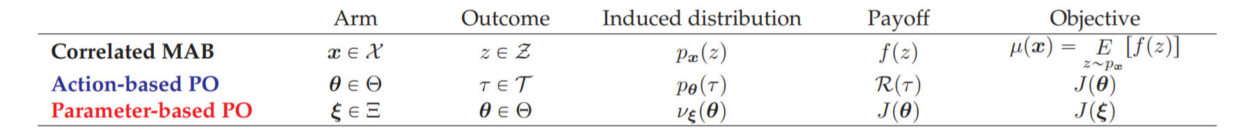
Figure 1: The Policy Optimisation problem formalization

Both cases are summarized in figure 1. The peculiarity of this framework, compared to the classic MAB one, is the special structure existing over the arms. In particular, the expected payoff $\mu$ of different arms is correlated thanks to the stochasticity of $p_{\bm{x}}$ on a common sample space $\mathcal{Z}$. In the following, we will use multiple importance sampling to exploit this correlation and guarantee efficient exploration.

2.2 Robust Multiple Importance Sampling Estimation

Importance sampling is a technique that allows estimating the expectation of a function under some target or proposal distribution with samples drawn from a different distribution, called behavioral.

Let $\mathit{P}$ and $\mathit{Q}$ be probability measures on a measurable space $(\mathcal{Z},\mathcal{F}$, such that $\mathit{P}\ll\mathit{Q}$ (i.e., $\mathit{P}$ is absolutely continuous w.r.t. $\mathit{Q}$). Let $p$ and $q$ be the densities of $\mathit{P}$ and $\mathit{Q}$, respectively, w.r.t. a reference measure, and the importance weight $\omega_{P/Q}=\frac{p}{q}$. Given a bounded function $f:\mathcal{Z}\rightarrow\mathbb{R}$, and a set of i.i.d. outcomes $z_{1},...,z_{N}$ sampled from $\mathit{Q}$, the importance sampling estimator of $\mu:=\mathbb{E}_{z\sim P}[f(z)]$ is:

$$\widehat{\mu}_{IS}:=\frac{1}{N}\sum_{i=1}^{N}\omega_{P/Q}(z_{i})f(z_{i})$$ (2)

which is an unbiased estimator, i.e., $\mathbb{E}_{z_{i}\overset{\text{iid}}{\sim}Q}[\widehat{\mu}_{IS}]=\mu$.

Multiple importance sampling is a generalization of the importance sampling technique which allows samples drawn from several different behavioral distributions to be used for the same estimate. Let $\mathit{Q}_{1},\dots,\mathit{Q}_{K}$ be all probability measures over the same probability space as $\mathit{P}$, and $\mathit{P}\ll\mathit{Q}_{k}$ for $k=1,\dots,K$. Given $N_{k}$ i.i.d. samples from each $\mathit{Q}_{k}$, the Balance Heuristic Multiple Importance Sampling (MIS) estimator is:

$$\widehat{\mu}_{BH}:=\sum_{k=1}^{K}\sum_{i=1}^{N_{k}}\frac{p(z_{ik})}{\sum_{j=1}^{K}N_{j}q_{j}(z_{ik})}f(z_{ik})$$ (3)

which is also an unbiased estimator of $\mu$.

Recently it has been observed that, in many cases of interest, the plain estimators 2 and 3 present problematic tail behaviors, preventing the use of exponential concentration inequalities. A common heuristic to address this problem consists in truncating the weights :

$$\breve{\mu}_{IS}:=\frac{1}{N}\sum_{i=1}^{N}\min\{M,\omega_{P/Q}(z_{i})\}f(z_{i})$$ (4)

where $M$ is a threshold to limit the magnitude of the importance weight. Similarly, for the multiple importance sampling case, restricting to the BH, we have:

$$\breve{\mu}_{BH}:=\frac{1}{N}\sum_{k=1}^{K}\sum_{i=1}^{N_{k}}\min\left\{M,\frac{p(z_{ik})}{\sum_{j=1}^{K}\frac{N_{j}}{N}q_{j}(z_{ik})}\right\}f(z_{ik})$$ (5)

Clearly, since we are changing the importance weights, we introduce a bias term, but, by reducing the range of the estimate, we get a benefit in terms of variance.

Intuitively, we can allow larger truncation thresholds M as the number of samples $N$ increases. The results from Papini et al. (2019) state that, when using an adaptive threshold depending on $N$, we are able to reach exponential concentration: with at least probability $1-\delta$, we have:

$$\breve{L}(\delta)\leq\mu\leq\breve{U}(\delta)$$

with:

$$\breve{U}(\delta)=\breve{\mu}_{BH}+\left\|f\right\|_{\infty}\left(\sqrt{2}+\frac{4}{3}\right)\left(\frac{d_{2}(P\|\Phi)\log(\frac{2}{\delta})}{N}\right)^{\frac{1}{2}}$$ (6)

and

$$\breve{L}(\delta)=\breve{\mu}_{BH}-\left\|f\right\|_{\infty}\left(\sqrt{2}+\frac{1}{3}\right)\left(\frac{d_{2}(P\|\Phi)\log(\frac{2}{\delta})}{N}\right)^{\frac{1}{2}}$$ (7)

such that:

$$d_{2}(P\|\Phi)=\int_{\mathcal{Z}}\left(\omega_{P/\Phi}\right)^{2}d\Phi=\mathbb{V}ar_{z\sim\Phi}\left[\omega_{P/\Phi}(z)\right]+1$$

$$\Phi=\sum_{j=1}^{K}\frac{N_{j}}{N}Q_{j}~{}~{}\text{is a mixture model}$$

and finally $\breve{\mu}_{BH}$ is the truncated balance heuristic estimator as defined in 5, using $N_{k}$ i.i.d. samples from each $Q_{k}$ and $M_{N}=\left(\frac{Nd_{2}(P\|\Phi)}{\log(\frac{1}{\delta})}\right)^{\frac{1}{2}}$ with $N=\sum_{j=1}^{K}N_{k}$

3 Problem Formalization

In this section, we will present the conservative exploration formalization with respect to The Policy Optimization Problem defined in 2.1. But first, we need to make two assumptions on the baseline arm.

Assumption 1.

We suppose that the baseline arm $\bm{x}_{b}$ is parametrized i.e. $\bm{x}_{b}\in\mathcal{X}$

In action-based PO, this is equivalent to supposing that there exists a parameter $\theta_{b}$ such that the baseline policy $\pi_{b}$ is $\pi_{b}=\pi_{\theta_{b}}$.
In parameter-based PO, this is equivalent to supposing that there exists a parameter $\xi_{b}$ such that the baseline hyperpolicy $\nu_{b}$ is $\nu_{b}=\nu_{\xi_{b}}$.
In both cases, it is always interesting to find a parameter space that contains the baseline.

Assumption 2.

We will initially assume that the algorithms know $\mu_{b}$ the expected reward of the default arm ($\mu_{b}=\mu(\bm{x}_{b})$).

This is reasonable in situations where the default action has been used for a long time and is well-characterized.

In PO, we will use this form of conservative constraint:

$$\forall t\in\left\{1,\dots,T\right\}~{}~{}\sum_{i=0}^{t-1}\mu(\bm{x}_{i})\geq(1-\alpha)t\mu(\bm{x}_{b})$$ (8)

for some $\alpha\in[0,1]$
and budget:

$$B_{t}=\sum_{i=0}^{t-1}\mu(\bm{x}_{i})-(1-\alpha)t\mu(\bm{x}_{b})$$ (9)

In action-based PO, this is equivalent to the constraint defined by Garcelon et al. (2020a) in the finite horizon case, since in action-based PO, $\mu(x_{i})=J(\theta_{i})=V^{\pi_{\theta_{i}}}(s)$ if we always start from the same initial state s, or $\mu(x_{i})=\mathbb{E}_{s\sim\rho}\left[V^{\pi_{\theta_{i}}}(s)\right]$ if $\rho$ is the distribution of initial states.

The requirement in 8 is often too strict in practice. We could relax the constraint by only verifying the condition 8 at some “checkpoints”. A simple case is where the checkpoints are equally spaced every $C^{h}$ steps.

$$\forall k>0~{}~{}\sum_{i=0}^{kC^{h}-1}\mu(\bm{x}_{i})\geq(1-\alpha)~{}kC^{h}\mu(\bm{x}_{b})$$ (10)

In order to determine whether an action at t is safe at a time $t\in[kC^{h},(k+1)C^{h}-1]$ of a phase $k\in\mathbb{N}$, we want to ensure that by playing the baseline arm until the next checkpoint (i.e., until $(k+1)C^{h}-1$) , the algorithm would meet the condition 10. Formally, at any step $t$, we replace 10 with:

$$\forall t>0~{}~{}\sum_{i=0}^{t}\mu(\bm{x}_{i})+\alpha((k+1)C^{h}-1-t)\mu(\bm{x}_{b})\geq(1-\alpha)~{}(t+1)\mu(\bm{x}_{b})$$ (11)

Our objective is to design algorithms that maximize the cumulative reward 1 while simultaneously satisfying the constraint 8 (or 11). The Conservative Policy optimization problem is then:

$$\max_{\bm{x}_{0},\dots,\bm{x}_{T}\in\mathcal{X}}\sum_{t=0}^{T}\mathbb{E}_{z_{t}\sim p_{\bm{x}_{t}}}[f(z_{t})]=\max_{\bm{x}_{0},\dots,\bm{x}_{T}\in\mathcal{X}}\sum_{t=0}^{T}\mu(\bm{x}_{t})$$

such that:

$$\forall t\in\left\{1,\dots,T\right\}~{}~{}\sum_{i=0}^{t-1}\mu(\bm{x}_{i})\geq(1-\alpha)t\mu(\bm{x}_{b})$$

4 Algorithms

In this section, we will propose algorithms that use use the mathematical tools presented in the Preliminaries 2 to build an optimistic estimation of $\mu$, choose the most optimistic arm, play that arm if is safe (by checking if a lower bound on the budget 9 is positif) or otherwise play the baseline arm.

Like discussed in Preliminaries 2, we will use robust multiple importance sampling to capture the correlation among the arms. To simplify the notation, we treat each sample $\bm{x}$ as a distinct one and corresponds to the case $K=t-1$ and $N_{k}=1$. Hence, at each iteration t:

$$\check{\mu}_{t}(\bm{x})=\sum_{k=0}^{t-1}\min\left\{M_{t},\frac{p_{\bm{x}}(z_{k})}{\sum_{j=0}^{t-1}p_{\bm{x}_{j}}(z_{k})}\right\}f(z_{k})$$ (12)

where $M_{t}=\left(\frac{td_{2}(P\|\Phi_{t})}{\log(\frac{2}{\delta_{t}})}\right)^{\frac{1}{2}}$ and $\Phi_{t}=\frac{1}{t}\sum_{k=0}^{t-1}p_{\bm{x}_{k}}$ and

$$\check{U}_{t}(\bm{x},\delta_{t}):=\check{\mu}_{t}(\bm{x})+\left\|f\right\|_{\infty}\left(\sqrt{2}+\frac{4}{3}\right)\left(\frac{d_{2}(p_{\bm{x}}\|\Phi_{t})\log(\frac{2}{\delta_{t}})}{t}\right)^{\frac{1}{2}}$$ (13)

$$\check{L}_{t}(\bm{x},\delta_{t}):=\check{\mu}_{t}(\bm{x})-\left\|f\right\|_{\infty}\left(\sqrt{2}+\frac{1}{3}\right)\left(\frac{d_{2}(p_{\bm{x}}\|\Phi_{t})\log(\frac{2}{\delta_{t}})}{t}\right)^{\frac{1}{2}}$$ (14)

are upper and lower bounds respectively on $\mu(x)$ with probability $1-\delta_{t}$.

Since $\mu_{b}$ is supposed known, we take:

$$\forall t~{}~{}\check{U}(\bm{x}_{b},\delta_{t})=\check{L}(\bm{x}_{b},\delta_{t})=\mu_{b}$$ (15)

In this context, in order to check with high probability that the conservative constraint is verified, we check that a lower-bound on the budget is positif. Pseudo-code for this first version is Algorithm 1

Algorithm 1 Conservative OPTIMIST

1:Input: $\bm{x}_{b}$, $\mu_{b}$, $(\delta_{t})_{t=1}^{T}$

2:Draw sample $z_{0}\sim p_{\bm{x}_{b}}$ and observe $f(z_{0})$

3:for $t=1,\dotsc,T$ do

4:     Select arm $\bm{x}_{t}\in\arg\max_{\bm{x}\in\mathcal{X}}\check{U}(\bm{x},\delta_{t})$

5:     $\check{B}_{t}\leftarrow\sum_{i=0}^{t-1}\check{L}_{t}(\bm{x}_{i},\delta_{t})+\check{L}_{t}(\bm{x}_{t},\delta_{t})-(1-\alpha)(t+1)\mu(\bm{x}_{b})$

6:     if $\check{B}_{t}\geq 0$ then

7:         Draw sample $z_{t}\sim p_{\bm{x}_{t}}$ and observe $f(z_{t})$

8:     else

9:         Draw sample $z_{t}\sim p_{\bm{x}_{b}}$ and observe $f(z_{t})$

10:     end if

11:end for

We can improve the limitation of having a two-step selection strategy by calculating first the set of safe arms (arms that verify that the budget is positif), then take the most optimistic arm from this set. This strategy yields more reward while still being conservative. Figure 2 (taken from Garcelon et al. (2020b) ) shows an example to build the intuition for this. The pseudo-code for it is in Algorithm 2

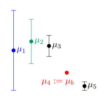
Figure 2: The OPTIMIST arm in blue does not satisfy the conservative condition, thus Alogithm 1 will play the basline action. However, arm2 and arm3 are considered ”safe arm” . And the Algorithm 2 will choose arm2; which is still conservative, and yields less regret than the baseline (arm chosen by Alogithm 1)

Algorithm 2 Improved Conservative OPTIMIST

1:Input: $\bm{x}_{b}$, $\mu_{b}$, $(\delta_{t})_{t=1}^{T}$

2:Draw sample $z_{0}\sim p_{\bm{x}_{b}}$ and observe $f(z_{0})$

3:for $t=1,\dotsc,T$ do

4:     $\check{B}_{t}(\bm{x})=\sum_{i=0}^{t-1}\check{L}_{t}(\bm{x}_{i},\delta_{t})+\check{L}_{t}(\bm{x},\delta_{t})-(1-\alpha)(t+1)\mu(\bm{x}_{b})$

5:     $\mathcal{C}_{t}=\left\{\bm{x}\in\mathcal{X}:\check{B}_{t}(\bm{x})\geq 0\right\}$

6:     Select arm $\bm{x}_{t}\in\arg\max_{\bm{x}\in\mathcal{C}_{t}}\check{U}(\bm{x},\delta_{t})$

7:     Draw sample $z_{t}\sim p_{\bm{x}_{t}}$ and observe $f(z_{t})$

8:end for

The optimization step (line 4 in 1 or lines 5 and 6 in 3) may be very difficult when X is not discrete as $\check{U}(\bm{x},\delta_{t})$ is non-convex and non-differentiable. Global optimization methods could be applied at the cost of giving up theoretical guarantees. In practice, this direction may be beneficial, but instead, like proposed by Papini et al. (2019), we could adapt to the compact case by using a general discretization method. The key intuition is to make the discretization progressively finer. The pseudocode for this variant is:

Algorithm 3 Improved Conservative OPTIMIST 2

1:Input: $\bm{x}_{b}$, $\mu_{b}$, $(\delta_{t})_{t=1}^{T}$, discretization schedule $(\tau_{t})_{t=1}^{T}$

2:Draw sample $z_{0}\sim p_{\bm{x}_{b}}$ and observe $f(z_{0})$

3:for $t=1,\dotsc,T$ do

4:     $\check{B}_{t}(\bm{x})=\sum_{i=0}^{t-1}\check{L}_{t}(\bm{x}_{i},\delta_{t})+\check{L}_{t}(\bm{x},\delta_{t})-(1-\alpha)(t+1)\mu(\bm{x}_{b})$

5:     Discretize $\mathcal{X}$ with a uniform grid $\tilde{\mathcal{X}}_{t}$ of $\tau_{t}^{d}$ points

6:     $\tilde{\mathcal{C}_{t}}=\left\{\bm{x}\in\tilde{\mathcal{X}}_{t}:\check{B}_{t}(\bm{x})\geq 0\right\}$

7:     Select arm $\bm{x}_{t}\in\arg\max_{\bm{x}\in\tilde{\mathcal{C}_{t}}}\check{U}(\bm{x},\delta_{t})$

8:     Draw sample $z_{t}\sim p_{\bm{x}_{t}}$ and observe $f(z_{t})$

9:end for

5 Regret Analysis

Let $Regret(T)=\sum_{i=0}^{T}\Delta_{t}$ be the total regret with $\Delta_{t}=\mu(\bm{x}^{\star})-\mu(\bm{x}_{t})$ and $\bm{x}^{\star}\in\arg\max_{\bm{x}\in\mathcal{X}}\mu(\bm{x})$.

In the following, we will show that Algorithm 1 yields sublinear regret under some mild assumptions (same assumptions as in Papini et al. (2019)). The proofs combine techniques from Papini et al. (2019) and Wu et al. (2016) and are reported in Appendix . First, we need the following assumption on the Renyi divergence:

Assumption 3.

We suppose that the 2-Rényi divergence is uniformely bounded:

$$\sup_{\bm{x}_{0},\dots,\bm{x}_{T}\in\mathcal{X}}d_{2}(p_{\bm{x}_{t}}\|\Phi_{t}):=v_{\epsilon}<\infty$$ (16)

with $\Phi_{t}=\frac{1}{t}\sum_{k=0}^{t-1}p_{\bm{x}_{k}}$

5.1 Discrete arm set

The case of the discrete arm set ($\left|\mathcal{X}\right|=K\in\mathbb{N}$), besides being convenient for the analysis, is also of practical interest: Even in applications where $\mathcal{X}$ is naturally continuous (e.g., robotics), the set of solutions that can be actually tried in practice may sometimes be constrained to a discrete, reasonably small, set. In this simple setting, Algorithm 1 achieves a regret $\tilde{\mathcal{O}}\left(\sqrt{T}\right)$:

Theorem 4.

With probability $1-\delta$, Algorithm 1 with confidence schedule $\delta_{t}=\frac{6\delta}{t^{2}\pi^{2}K}$, satisfies the following:

$$\forall t\in\left\{1,\dots,T+1\right\}~{}~{}\sum_{i=0}^{t-1}\mu(\bm{x}_{i})\geq(1-\alpha)t\mu(\bm{x}_{b})$$ (17)

$$Regret(T)\leq\Delta_{b}+2\sqrt{LT}+\frac{\left\|f\right\|_{\infty}\Delta_{b}}{\alpha\mu_{b}}+\frac{4KL}{\alpha\mu_{b}}$$ (18)

with $L=(a+b)^{2}v_{\epsilon}[2\log(T)+\log(\frac{\pi^{2}K}{3\delta})]$,
$a=\left\|f\right\|_{\infty}\left(\sqrt{2}+\frac{4}{3}\right)$ and $b=\left\|f\right\|_{\infty}\left(\sqrt{2}+\frac{1}{3}\right)$

This yields a $\tilde{\mathcal{O}}(\sqrt{T})$ regret.

5.2 Compact arm set

We consider the more general case of a compact arm set $\mathcal{X}$. We assume that $\mathcal{X}$ is entirely contained in a box $\left[-D,D\right]^{d}$, with $D\in\mathbb{R}_{+}$. We also need the following assumption on the expected payoff:

Assumption 5.

The expected payoff $\mu$ is Lipschitz continuous, i.e., there exists a constant $P>0$ such that, for every $\bm{x},\bm{x^{\prime}}\in\mathcal{X}$ :

$$\left|\mu(\bm{x})-\mu(\bm{x^{\prime}})\right|\leq P\left\|\bm{x}-\bm{x^{\prime}}\right\|_{1}$$ (19)

Theorem 6.

Under Assumptions 16 and 19, Algorithm 3 with confidence schedule $\delta_{t}=\frac{6\delta}{t^{2}\pi^{2}\left(1+\left\lceil t^{\frac{1}{2}}\right\rceil^{d}\right)}$ and discretization schedule $\tau_{t}=\left\lceil t^{\frac{1}{2}}\right\rceil$ guarantees, with probability at least $1-\delta$:

$$\forall t\in\left\{1,\dots,T+1\right\}~{}~{}\sum_{i=0}^{t-1}\mu(\bm{x}_{i})\geq(1-\alpha)t\mu(\bm{x}_{b})$$ (20)

$$Regret(T)\leq\Delta_{b}+2\sqrt{L^{\prime}T}+\frac{\left\|f\right\|_{\infty}\Delta_{b}}{\alpha\mu_{b}}+\frac{8L^{\prime}}{\alpha\mu_{b}}$$ (21)

with $L^{\prime}=((a+b)v_{\epsilon}^{\frac{1}{2}}\left[\left(2+\frac{d}{2}\right)\log(T)+d\log(2)+\log(\frac{\pi^{2}}{3\delta})\right]^{\frac{1}{2}}$

$+PDd)^{2}$ ,
$a=\left\|f\right\|_{\infty}\left(\sqrt{2}+\frac{4}{3}\right)$ and $b=\left\|f\right\|_{\infty}\left(\sqrt{2}+\frac{1}{3}\right)$

Algorithm 3 achieves a regret $\tilde{\mathcal{O}}\left(d\sqrt{T}\right)$: Unfortunately, the time required for optimization is exponential in arm space dimensionality $d$.

6 Experiments

In this section, we evaluate Algorithm 1 compared to CUCRL (Garcelon et al. (2020a)) on the stochastic inventory control problem (Puterman (1994), Sec. 3.2.1): at the beginning of each month t, a manager has to decide the number of items to order (maximum capacity $M=6$ in order to satisfy a uniform random demand when taking into account ordering and inventory maintenance costs. The optimal policy belongs to the set of thresholds policies characterized by parameters $(\sigma,\Sigma)$ where $\Sigma$ is the target stock and $\sigma$ is the capacity threshold. As a baseline, we decided to take the threshold policy $(\sigma,\Sigma)=(4,4)$, while the optimal one verifies $(\sigma^{\star},\Sigma^{\star})=(3,6)$. Experiments are run for $T=10000$ time steps and a conservative level $\alpha=0.1$, and results displayed in figure 3 are averaged over 20 realizations.

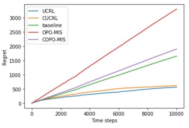
Figure 3: Implementation of OPTIMIST, Conservative OPTIMIST, UCRL, CUCRL on the inventory problem

As expected, we can see that the CUCRL algorithm converges a little bit slower than UCRL due to the conservative constraint restricting a free exploration of the environment. However, OPO-MIS (Optimistic Policy Optimization with Multiple Importance Sampling) adapted from https://github.com/WolfLo/optimist performs really poorly with a linear regret worse than the baseline. This is essentially explained by the authors choice to design linear actor policies in their implementation of the method which is clearly not suitable for this particularly non-linear inventory problem (as the optimal policy is a threshold one). Nonetheless, adding the conservative constraint with COPO-MIS 1 (Conservative Optimistic Policy Optimization with Multiple Importance Sampling) enables to not diverge much from the baseline policy and yields a quite similar regret, showing that the conservative constrain is well respected when using 1, and justifying the necessity to add safety constraints when the learning algorithm (OPTIMIST) fails to find a good policy.

7 Conclusion

In this work, we have studied the problem of conservative exploration in policy optimization using MAB techniques. We have used algorithmic ideas from Papini et al. (2019) to propose an online model free algorithm that solves the problem of conservative exploration in RL as defined in Garcelon et al. (2020a), both the action-based and the parameter-based exploration frameworks, and for both discrete and continuous parameter spaces. We have proved sublinear regret bounds for Conservative OPTIMIST under assumptions that are easily met in practice. The empirical evaluation on the inventory problem showed that the proposed algorithm respect effectively the conservative constraint. However, since the parametrization of the policies (linear policies) in the implementation of Papini et al. (2019) was not adapted to the inventory case, OPTIMIST failed to reach a good policy. Future work should focus on finding more efficient parametrization of the policies in the code implementation, but also ways to perform effectively optimization in the infinite-arm setting.

Appendix

Appendix A Proof of Theorem 4

Proof.

With probability $1-\delta_{t}$ :

$$\mu(\bm{x})\in\left[\check{L}_{t}(\bm{x},\delta_{t}),\check{U}_{t}(\bm{x},\delta_{t})\right]~{}~{}\forall\bm{x}\in\mathcal{X}~{}\forall t\in\left\{1,\dots,T\right\}$$ (22)

To ease notation, we will rewrite 22 as:

$$\check{\mu}_{t}(\bm{x})-\mu(\bm{x})\in\left[-a\beta_{t}(\bm{x},\delta_{t}),b\beta_{t}(\bm{x},\delta_{t})\right]~{}~{}\forall\bm{x}\in\mathcal{X}~{}\forall t\in\left\{1,\dots,T\right\}$$

with $a:=\left\|f\right\|_{\infty}\left(\sqrt{2}+\frac{4}{3}\right)$ and $b:=\left\|f\right\|_{\infty}\left(\sqrt{2}+\frac{1}{3}\right)$ and $\beta_{t}(\bm{x},\delta_{t}):=\left(\frac{d_{2}(p_{\bm{x}}\|\Phi_{t})\log(\frac{2}{\delta_{t}})}{t}\right)^{\frac{1}{2}}$

We take:
$F=\bigcap_{k=1}^{K}\bigcap_{t=1}^{T}\left\{\check{\mu}_{t}(\bm{x}_{k})-\mu(\bm{x}_{k})\in\left[-a\beta_{t}(\bm{x},\delta_{t}),b\beta_{t}(\bm{x},\delta_{t})\right]\right\}$

With $\delta_{t}=\frac{6\delta}{t^{2}\pi^{2}K}$, we have: $\mathbb{P}(F)$

$$=1-\mathbb{P}\left(\bigcup_{k=1}^{K}\bigcup_{t=1}^{T}\left\{\check{\mu}_{t}(\bm{x}_{k})-\mu(\bm{x}_{k})\in\left[-a\beta_{t}(\bm{x},\delta_{t}),b\beta_{t}(\bm{x},\delta_{t})\right]\right\}\right)$$

$$\geq 1-K\sum_{t=1}^{T}\delta_{t}$$

$$\geq 1-K\sum_{t=1}^{T}\frac{6\delta}{t^{2}\pi^{2}K}$$

$$\geq 1-\delta$$

since $\sum_{t=1}^{T}\frac{1}{t^{2}}\leq\sum_{t=1}^{\infty}\frac{1}{t^{2}}=\frac{\pi^{2}}{6}$.

If $x_{t}$ is an arm chosen by OPTIMIST, with probability $1-\delta$ we have: :

$$\Delta_{t}=\mu(\bm{x}^{\star})-\mu(\bm{x}_{t})\leq\check{\mu}_{t}(\bm{x}^{\star})+a\beta_{t}(\bm{x}^{\star},\delta_{t})-\mu(\bm{x}_{t})$$ (23)

$$\leq\check{\mu}_{t}(\bm{x}_{t})+a\beta_{t}(\bm{x}_{t},\delta_{t})-\mu(\bm{x}_{t})$$ (24)

$$\leq(a+b)\beta_{t}(\bm{x}_{t},\delta_{t})=(a+b)\left(\frac{d_{2}(p_{\bm{x}}\|\Phi_{t})\log(\frac{2}{\delta_{t}})}{t}\right)^{\frac{1}{2}}$$ (25)

$$\leq(a+b)v_{\epsilon}^{\frac{1}{2}}\left(\frac{2\log(t)+\log(\frac{\pi^{2}K}{3\delta})}{t}\right)^{\frac{1}{2}}$$ (26)

$$\leq(a+b)v_{\epsilon}^{\frac{1}{2}}\left(\frac{2\log(T)+\log(\frac{\pi^{2}K}{3\delta})}{t}\right)^{\frac{1}{2}}$$ (27)

$$\leq\sqrt{\frac{L}{t}}$$ (28)

with $L=(a+b)^{2}v_{\epsilon}[2\log(T)+\log(\frac{\pi^{2}K}{3\delta})]$

Now, we will try to find a bound on the number of times a sub-optimal arm $k$ has been chosen till T: $T_{k}(T)=\sum_{i=0}^{t}\mathbb{1}_{x_{t}=x_{k}}$. If the arm is never chosen, $T_{k}(T)=0$ If it is at least chosen once, let $t$ be the last time $x_{k}$ has been chosen ($x_{k}=x_{t}$), by 28 we have:

$$T_{k}(T)\leq t\leq\frac{L}{{\Delta_{t}}^{2}}=\frac{L}{{\Delta_{k}}^{2}}$$ (29)

The regret can be written as:

$$Regret(T)=\sum_{t=0}^{T}\Delta_{t}$$

$$=\sum_{{t=1},t\in\mathcal{S}_{T}}^{T}\Delta_{t}~{}+T_{b}(T)\Delta_{b}$$

with $\mathcal{S}_{T}=\left\{t\in\left\{1,\dots,T\right\}:x_{t}\neq x_{b}\right\}$ the set of times where the OPTIMIST action was chosen (at t=0 we always choose $x_{b}$), $T_{k}(T)=\sum_{t=0}^{T}\mathbb{1}_{x_{t}=x_{k}}$ the number of times the arm k was chosen till time $T$, and $T_{b}(T)=\sum_{t=0}^{T}\mathbb{1}_{x_{t}=x_{b}}$ the number of time the baseline arm was chosen till times $T$.

With probability $1-\delta$, we have:

$$\sum_{{t=1},t\in\mathcal{S}_{T}}^{T}\Delta_{t}$$

$$\leq\sum_{{t=1},t\in\mathcal{S}_{T}}^{T}\sqrt{\frac{L}{t}}$$

$$\leq 2\sqrt{L}\sqrt{T}$$

If $\Delta_{b}=0$ then the theorem holds trivially; we therefore assume that $\Delta_{b}>0$ and find an upper bound for $T_{b}(T)$.

Let $\tau=\max\left\{t\leq T~{}|~{}x_{t}=x_{b}\right\}$ be the last round in which the default arm is played. Since $F$ holds and $\check{U}(\bm{x}_{b},\delta_{t})=\mu_{b}<\mu^{*}<\max_{i}\theta_{i}(t)$, it follows that $x_{b}$ is never the OPTIMIST choice and the default arm was only played because $\check{B}_{\tau}<0$:

$$\sum_{k=1,\bm{x}_{k}\neq\bm{x}_{b}}^{K}T_{k}(\tau)\check{L}(\bm{x}_{k},\delta_{t})+T_{b}(\tau-1)\mu(\bm{x}_{b})-(1-\alpha)(\tau+1)\mu(\bm{x}_{b})<0$$ (30)

we replace $\tau=\sum_{k=1,\bm{x}_{k}\neq\bm{x}_{b}}^{K}T_{k}(\tau)+T_{b}(\tau-1)$ in this inequality and rearrange, we have then:

$$\alpha T_{b}(\tau-1)\mu(\bm{x}_{b})$$

$$<(1-\alpha)\mu(\bm{x}_{b})+\sum_{k=1,\bm{x}_{k}\neq\bm{x}_{b}}^{K}T_{k}(\tau)\left(\left(1-\alpha\right)\mu(\bm{x}_{b})-\check{L}(\bm{x}_{k},\delta_{t})\right)$$

$$\leq(1-\alpha)\mu(\bm{x}_{b})+$$

$$\sum_{k=1,\bm{x}_{k}\neq\bm{x}_{b}}^{K}T_{k}(\tau)\left(\left(1-\alpha\right)\mu(\bm{x}_{b})-\mu_{k}+(a+b)\beta_{\tau}(\bm{x}_{k},\delta_{\tau})\right)$$

$$\leq\left\|f\right\|_{\infty}+\sum_{k=1,\bm{x}_{k}\neq\bm{x}_{b}}^{K}T_{k}(\tau)\left(\left(1-\alpha\right)\mu(\bm{x}_{b})-\mu_{k}+\sqrt{\frac{L}{T_{k}(\tau)}}\right)$$

$$\leq\left\|f\right\|_{\infty}+\sum_{k=1,\bm{x}_{k}\neq\bm{x}_{b}}^{K}a_{k}T_{k}(\tau)+\sqrt{LT_{k}(\tau)}$$

$$\leq\left\|f\right\|_{\infty}+\sum_{k=1,\bm{x}_{k}\neq\bm{x}_{b}}^{K}S_{k}$$

with $S_{k}=a_{k}T_{k}(\tau)+\sqrt{LT_{k}(\tau)}$ and $a_{k}=\left(1-\alpha\right)\mu(\bm{x}_{b})-\mu_{k}$ to ease notation.

We have two cases: $a_{k}>0$ or $a_{k}\leq 0$.

If $a_{k}>0$: then $\mu_{k}<\left(1-\alpha\right)\mu(\bm{x}_{b})$ so arm $k$ is suboptimal and by 29, we have: $T_{k}(\tau)\leq T_{k}(T)\leq\frac{L}{{\Delta_{k}}^{2}}$ so then:
$S_{k}\leq a_{k}\frac{L}{{\Delta_{k}}^{2}}+\frac{L}{{\Delta_{k}}}\leq\frac{2L}{{\Delta_{k}}}$ (because $a_{k}\leq\Delta_{k}$).

If $a_{k}\leq 0$: $S_{k}=a_{k}T_{k}(\tau)+\sqrt{LT_{k}(\tau)}\leq-\frac{L}{4a_{k}}=\frac{L}{4(\Delta_{b}+\alpha\mu_{b}-\Delta_{k})}$ by using $ax^{2}+bx\leq-\frac{b^{2}}{4a}$ when $a\leq 0$.

We can combine both by taking:

$$S_{k}\leq\frac{2L}{{\max(\Delta_{k},\Delta_{b}-\Delta_{k})}}\leq\frac{4L}{\Delta_{b}}$$

($\mu_{b}\geq 0$ and $\max(\Delta_{k},\Delta_{b}-\Delta_{k})\geq\frac{\Delta_{b}}{2}$).

Finally, we have:

$$T_{b}(T)=T_{b}(\tau-1)+1$$

$$\leq 1+\frac{\left\|f\right\|_{\infty}}{\alpha\mu_{b}}+\frac{4KL}{\alpha\Delta_{b}\mu_{b}}$$

To conclude, the regret can be bounded with probability $1-\delta$ by:

$$Regret(T)\leq 2\sqrt{LT}+\Delta_{b}+\frac{\left\|f\right\|_{\infty}\Delta_{b}}{\alpha\mu_{b}}+\frac{4KL}{\alpha\mu_{b}}$$

∎

Appendix B Proof of Theorem 6

Proof.

The only difference in this case is that 28 becomes:

$$\Delta_{t}\leq(a+b)\beta_{t}(\bm{x}_{t},\delta_{t})+\frac{PDd}{\tau_{t}}$$ (31)

(eq (64) from Papini et al. (2019), with $P$ the Lipshitz constant)

By replacing $\tau_{t}=\left\lceil t^{\frac{1}{2}}\right\rceil$ and $\delta_{t}=\frac{6\delta}{t^{2}\pi^{2}\left(1+\left\lceil t^{\frac{1}{2}}\right\rceil^{d}\right)}$ , we have:

$$\Delta_{t} \leq\frac{(a+b)v_{\epsilon}^{\frac{1}{2}}\left[\left(2+\frac{d}{2}\right)\log(T)+d\log(2)+\log(\frac{\pi^{2}}{3\delta})\right]^{\frac{1}{2}}}{\sqrt{t}}+\frac{PDd}{\sqrt{t}}$$

$$=\sqrt{\frac{L^{\prime}}{t}}$$

with

$$L^{\prime}=\left((a+b)v_{\epsilon}^{\frac{1}{2}}\left[\left(2+\frac{d}{2}\right)\log(T)+d\log(2)+\log(\frac{\pi^{2}}{3\delta})\right]^{\frac{1}{2}}+PDd\right)^{2}$$ (32)

In order to reuse the steps from the proof of Theorem 4, we need an independent discretization that does not depend on t (otherwise the number of arm at the end is exponential in T which breaks the regret).

To simplify the analyse, we will break the compact arm $\mathcal{X}$ into two regions (or ’big’ arms): A first one where $\left\{\bm{x}\in\mathcal{X}:\mu(\bm{x}^{\star})-\mu(\bm{x})\leq\epsilon\right\}$ (for a fixed $\epsilon>0$ chosen such that 30 could be exactly split into two terms), that contains the best arm, and a second region (suboptimal ’big’ arm) which is just $\left\{\bm{x}\in\mathcal{X}:\mu(\bm{x}^{\star})-\mu(\bm{x})>\epsilon\right\}$

Now, we can reususe the same steps from the previous proof, with two ’big’ arms, one optimal, and the other suboptimal. The same steps work exactly, with the only difference is having the new $L^{\prime}$ rather than $L$ and $K=2$.

The regret is then:

$$Regret(T)\leq\Delta_{b}+2\sqrt{L^{\prime}T}+\frac{\left\|f\right\|_{\infty}\Delta_{b}}{\alpha\mu_{b}}+\frac{8L^{\prime}}{\alpha\mu_{b}}$$ (33)

∎

References

• Garcelon et al. (2020a) Evrard Garcelon, Mohammad Ghavamzadeh, Alessandro Lazaric, and Matteo Pirotta. Conservative exploration in reinforcement learning. In Silvia Chiappa and Roberto Calandra, editors, Proceedings of the Twenty Third International Conference on Artificial Intelligence and Statistics, volume 108 of Proceedings of Machine Learning Research, pages 1431–1441. PMLR, 26–28 Aug 2020a. URL http://proceedings.mlr.press/v108/garcelon20a.html.
• Garcelon et al. (2020b) Evrard Garcelon, Mohammad Ghavamzadeh, Alessandro Lazaric, and Matteo Pirotta. Improved algorithms for conservative exploration in bandits, 2020b.
• Papini et al. (2019) Matteo Papini, Alberto Maria Metelli, Lorenzo Lupo, and Marcello Restelli. Optimistic policy optimization via multiple importance sampling. In Kamalika Chaudhuri and Ruslan Salakhutdinov, editors, Proceedings of the 36th International Conference on Machine Learning, volume 97 of Proceedings of Machine Learning Research, pages 4989–4999. PMLR, 09–15 Jun 2019. URL http://proceedings.mlr.press/v97/papini19a.html.
• Puterman (1994) Martin L. Puterman. Markov Decision Processes: Discrete Stochastic Dynamic Programming. John Wiley & Sons, Inc., New York, NY, USA, 1994. ISBN 0471619779.
• Wu et al. (2016) Yifan Wu, Roshan Shariff, Tor Lattimore, and Csaba Szepesvári. Conservative bandits, 2016.