The discovery of a highly accreting, radio-loud quasar at $z=6.82$

Abstract

Radio sources at the highest redshifts can provide unique information on the first massive galaxies and black holes, the densest primordial environments, and the epoch of reionization. The number of astronomical objects identified at $z>6$ has increased dramatically over the last few years, but previously only three radio-loud ($R_{2500}=f_{\nu,5\,\mathrm{GHz}}/f_{\nu,2500\,\text{\AA}}>10$) sources had been reported at $z>6$, with the most distant being a quasar at $z=6.18$. Here we present the discovery and characterization of PSO J172.3556+18.7734, a radio-loud quasar at $z=6.823$. This source has an Mg II-based black hole mass of $\sim 3\times 10^{8}\,M_{\odot}$ and is one of the fastest accreting quasars, consistent with super-Eddington accretion. The ionized region around the quasar is among the largest measured at these redshifts, implying an active phase longer than the average lifetime of the $z\gtrsim 6$ quasar population. From archival data, there is evidence that its 1.4 GHz emission has decreased by a factor of two over the last two decades. The quasar’s radio spectrum between 1.4 and 3.0 GHz is steep ($\alpha=-1.31$). Assuming the measured radio slope and extrapolating to rest-frame 5 GHz, the quasar has a radio-loudness parameter $R_{2500}\sim 90$. A second steep radio source ($\alpha=-0.83$) of comparable brightness to the quasar is only 23$\farcs$1 away ($\sim$120 kpc at $z=6.82$; projection probability $<2\%$), but shows no optical or near-infrared counterpart. Further follow-up is required to establish whether these two sources are physically associated.

1 Introduction

Radio jets from active galactic nuclei (AGNs) are thought to play a key role in the coevolution of supermassive black holes and their host galaxies, as well as in the early growth of massive black holes (e.g., Jolley & Kuncic, 2008; Volonteri et al., 2015; Hardcastle & Croston, 2020). Yet, strong radio emission seems to be a rare or at least short-lived phenomenon. Only about 10% of all quasars are strong radio emitters, almost independent of their redshifts up to $z\sim 6$ (e.g., Bañados et al. 2015; Yang et al. 2016; Shen et al. 2019 but see also Jiang et al. 2007; Kratzer & Richards 2015).

The radio-loudness of a quasar is usually defined as the ratio of rest-frame 5 GHz (radio) and 4400 Å (optical) flux densities ($R_{4400}$; e.g., Kellermann et al. 1989) although sometimes the 2500 Å (UV) emission is used instead of the optical flux density ($R_{2500}$; e.g., Jiang et al. 2007). For an unobscured type-1 quasar, the different definitions yield comparable results. An object is considered radio-loud if $R_{2500}$ or $R_{4400}$ is greater than 10. Radio-loud sources at the highest accessible redshifts are of particular interest for multiple reasons. For example, radio galaxies are known to be good tracers of overdense environments (e.g., Venemans et al., 2007; Wylezalek et al., 2013) and at high redshift these overdensities could be the progenitors of the galaxy clusters seen in the present-day universe (Overzier, 2016; Noirot et al., 2018). Furthermore, radio-loud sources deep in the epoch of reionization would enable crucial absorption studies of the intergalactic medium (IGM) at this critical epoch (e.g., Carilli et al., 2002; Ciardi et al., 2013; Thyagarajan, 2020) and they could potentially also constrain the nature of dark matter particles by detecting neutral hydrogen in absorption in the radio spectrum (e.g., Shimabukuro et al., 2020).

The number of astronomical objects known within the first billion years of the universe has increased dramatically over the last few years, with galaxies being discovered up to $z\sim 11$ (Oesch et al., 2014) and quasars up to $z\sim 7.5$ (Bañados et al., 2018b; Yang et al., 2020). On the other hand, identifying strong radio emitters at high redshift has been difficult. The highest-redshift radio galaxy lies at $z=5.7$ (Saxena et al., 2018), with the previous record at $z=5.2$ (van Breugel et al., 1999). Out of the 200 published quasars at $z>6$ (e.g., Bañados et al., 2016; Matsuoka et al., 2019a; Andika et al., 2020), only three are known to be radio-loud. For the large majority of the remainder, the existing radio data are too shallow to robustly classify them as radio-quiet or radio-loud, although there are on-going efforts to obtain deeper radio observations of these objects. The three $z>6$ radio-loud quasars currently known, listed by increasing redshift, are: J0309+2717 at $z=6.10$ (Belladitta et al., 2020), J1427+3312 at $z=6.12$ (McGreer et al., 2006; Stern et al., 2007), and J1429+5447 at $z=6.18$ (Willott et al., 2010a).

In this paper we present the discovery and initial characterization of the most distant radio-loud quasar currently known, PSO J172.3556+18.7734 (hereafter P172+18) at $z=6.823$, as measured from the Mg II  emission line. In Section 2 we describe the selection of the quasar and the details of follow-up observations. The properties derived from near-infrared spectroscopy are presented in Section 3 and the properties from follow-up radio observations are introduced in Section 4. We summarize and present our conclusion in Section 5. Throughout the paper we use a flat cosmology with $H_{0}=70\,\mbox{km\,s}^{-1}$ Mpc^-1, $\Omega_{M}=0.3$, and $\Omega_{\Lambda}=0.7$. In this cosmology the age of the universe at the redshift of P172+18 is 776 Myr and 1 pkpc corresponds to 5$\farcs$3. Optical and near-infrared magnitudes are reported in the AB system, while for radio observations we report the peak flux density unless otherwise stated. For nondetections we report $3\sigma$ upper limits.

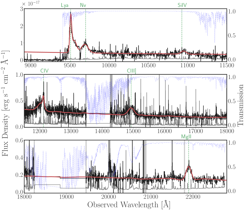
Figure 1: Optical/near-infrared spectrum of P172+18. The final spectrum was obtained by combining all the spectroscopic follow-up data available (Keck/NIRES, VLT/X-Shooter, and LBT/MODS).

2 A radio-loud quasar at $z=6.8$

2.1 Selection and Discovery

P172+18 has been identified as a $z>6.5$ quasar candidate by at least two independent methods. We first selected P172+18  as a $z$-dropout radio-loud candidate in Bañados et al. 2015 (see their Table 1). That selection required red ($z_{\rm P1}-y_{\rm P1}>1.4$) sources in the stacked object Pan-STARRS1 catalog (Chambers et al., 2016) and a counterpart in the radio survey Faint Images of the Radio Sky at Twenty cm (FIRST, Becker et al., 1995) to avoid most of the L- and T-dwarfs, which are the main contaminants for $z>6.5$ quasar searches (see Bañados et al. 2015 for details). The Pan-STARRS1 and FIRST measurements for P172+18 are listed in Table 1. This object also stands out as a promising high-redshift quasar candidate in a new method to select $z\gtrsim 6.5$ quasars exploiting the overlap of Pan-STARRS1 and the DESI Legacy Imaging Surveys (DECaLS; Dey et al. 2019), which will be presented in a forthcoming paper along with additional $z\gtrsim 6.5$ quasar discoveries (E. Bañados et al. in preperation). P172+18 was selected using the DECaLS DR7 catalog, but in Table 1 we report the photometry from the latest (DR8) data release.

The optical photometry of P172+18 in the DECaLS DR7 and DR8 catalogs is consistent. However, the mid-infrared Wide-fied Infrared Survey Explorer (WISE) magnitudes are inconsistent at the $2\sigma$ level even though DR7 and DR8 use the same input set of WISE images spanning from 2010 to 2017 (A. Meisner, private communication; Meisner et al., 2019). DECaLS provides matched WISE photometry by using the $g_{\rm DE}$, $r_{\rm DE}$, $z_{\rm DE}$ information to infer the WISE magnitudes from deep image coadds using all available WISE data (Lang, 2014; Meisner et al., 2017, 2019). The WISE DECaLS DR7 magnitudes are $W1=21.25\pm 0.21$ and $W2=21.30\pm 0.51$ in contrast to the DR8 magnitudes of $W1=20.71\pm 0.13$ and $W2=20.73\pm 0.31$. The main difference between DR7 and DR8 is the change of sky modeling as presented in Schlafly et al. (2019), which can affect the fluxes of sources at the faint limit of the unWISE coadds. Therefore, the reported WISE magnitudes need to be taken with caution.

We confirmed P172+18 as a $z\sim 6.8$ quasar on 2019 January 12 with a 450 s spectrum using the Folded-port InfraRed Echellete (FIRE; Simcoe et al. 2008, 2013) spectrograph in prism mode at the Magellan Baade telescope at Las Campanas Observatory. The spectrum had poor signal-to-noise ratio (S/N) but was sufficient to unequivocally identify P172+18 as the most distant radio-loud quasar known to date, which triggered a number of follow-up programs described below.

2.2 Near-infrared Imaging Follow-up

We obtained $JHK$ photometry using the NOTCam instrument at the Nordic Optical Telescope (Djupvik & Andersen, 2010). The total exposure times were 19 minutes each for $J_{\rm NOT}$ and $H_{\rm NOT}$ and 31 minutes for $Ks_{\rm NOT}$. Data reduction consisted of standard procedures: bias subtraction, flat-fielding, sky subtraction, alignment, and stacking. Table 2 presents a log of the observations.

We calculate the zero-points of the NOT observations, calibrating against stars in the Two Micron All Sky Survey (2MASS) using the following conversions:

$$J_{\rm NOT}= J_{\rm 2MASS}-0.074\times(J_{\rm 2MASS}-H_{\rm 2MASS})+0.003$$

$$H_{\rm NOT}= H_{\rm 2MASS}+0.045\times(J_{\rm 2MASS}-H_{\rm 2MASS})+0.006$$

$$Ks_{\rm NOT}= K_{\rm 2MASS}+0.580\times(H_{\rm 2MASS}-K_{\rm 2MASS})+0.225$$

These conversions were calculated via linear fits of the stellar loci as described in Section 2.6 of Bañados et al. (2014). The near-infrared photometry is listed in Table 1.

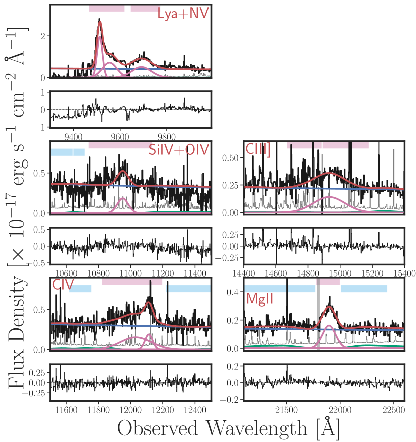
Figure 2: Zoom-in on the main broad emission lines from near-infrared spectroscopy. We show the total spectral fit (red line), and the different components, i.e. power law + Balmer pseudo-continuum (blue line), Fe II template (green line, from Vestergaard & Wilkes 2001), and emission lines (pink lines). Spectral regions used for the continuum and spectral line fits are shown as horizontal light blue and pink regions, respectively. The noise spectrum is reported in gray in the main panels, while residuals are also shown below each panel. Regions with low S/N or strong absorption features are masked out during the fit, and highlighted with gray vertical regions.

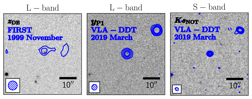
Figure 3: VLA L- and S-band observations (blue contours) centered on the position of P172+18 over optical and near-infrared imaging as labeled in the figure; north is up and east is left. Contours correspond to 3$\sigma$ and 5$\sigma$ for the FIRST image (left panel) and to 3$\sigma$, 7$\sigma$, 14$\sigma$, and 21$\sigma$ for the VLA-DDT images (corresponding negative contours for all panels are dashed); $\sigma$ for each of the radio images is listed in Table 2. The follow-up observations reveal a second radio source 23$\farcs$1 to the northwest of the quasar with no counterpart in available optical or near-infrared imaging (see Table 1). Although the secondary radio source is slightly brighter than the quasar in the deepest observations, it was not visible in the FIRST survey data.

2.3 Spectroscopic Follow-up

We obtained three follow-up spectra of P172+18. On 2019 February 18 we observed P172+18 for 3.5 hr with Keck/NIRES (Wilson et al., 2004). Between 2019 March 8 and April 8 we used the Very Lare Telescope (VLT)/X-Shooter spectrograph (Vernet et al., 2011) to observe the target for a total time of 3.5 hr. We also observed P172+18 with the Large Binocular Telescope (LBT)/Multi-Object Double Spectrograph (MODS) (Pogge et al., 2010) on 2019 June 13. The MODS observations were carried out in binocular mode for 20 minutes on-source. We summarize the spectroscopic follow-up observations in Table 3.

The Keck/NIRES and VLT/X-Shooter data were reduced with the Python Spectroscopic Data Reduction Pipeline (PypeIt; Prochaska et al., 2019, 2020). In practice, sky subtraction on the 2D images was obtained through a B-spline fitting procedure and differences between AB dithered exposures. The 1D spectrum was extracted with the optimal spectrum extraction technique (Horne, 1986). Each 1D single exposure was flux-calibrated using standard stars observed with X-Shooter. Then, the 1D spectra were stacked and a telluric model was fitted, obtained from telluric model grids from the Line-By-Line Radiative Transfer Model (LBLRTM4; Clough et al. 2005, Gullikson et al. 2014). The X-Shooter and NIRES spectra were then absolute-flux-calibrated with respect to the $J_{\mathrm{{NOT}}}$ magnitude (see Table 1). The LBT/MODS binocular spectra were reduced with IRAF using standard procedures, including bias subtraction, flat-fielding, and telluric and wavelength calibration. They were each scaled to the $y_{\rm P1}$ magnitude.

We performed all measurements presented in the following sections in the individual spectra, which resulted in consistent results. To maximize the information provided by all spectra we re-binned them to a common wavelength grid with a pixel size of 50 km s^-1, and averaged them weighting by their inverse variance. The final spectrum that we use for our main analysis is shown in Figure 1 and a zoom-in on the main emission lines is presented in Figure 2.

2.4 Radio Follow-up

Follow-up radio-frequency observations were carried out with the Karl G. Jansky Very Large Array (VLA) of the NRAO on 2019 March 5 and 2019 March 11, in S and L bands respectively. Each observing session was 1 hr in total ($\sim$21 min on-source). The VLA was in B-configuration with a maximum baseline length of 11.1 km. The observations spanned the frequency ranges 1–2 GHz (L band; center frequency 1.5 GHz) and 2–4 GHz (S band; center frequency 3 GHz). The WIDAR correlator was configured to deliver 16 adjacent subbands per receiver band, each 64 MHz at L band and 128 MHz at S band. Each subband had 64 spectral channels, resulting in 1 MHz channels in the L-band data and 2 MHz channels in the S-band data.

The source 3C 286 (J1331+3030) was used to set the absolute flux density scale and to calibrate the bandpass response, and the compact source J1120+1420 was observed as the complex gain calibrator. Data editing, radio-frequency interference (RFI) excision, calibration, imaging, and analysis were performed using the Common Astronomy Software Applications (CASA) package of the NRAO. The data were calibrated using the CASA pipeline version 5.4.1-23, and the continuum images were made using the wide-field w-projection gridder and Briggs weighting with robust=0.4 as implemented in the CASA task tclean. Due to the excision of data affected by RFI, the resulting L- and S-band images have the reference frequencies of 1.52 and 2.87 GHz, respectively. The resulting beam sizes for the 1.52 and 2.87 GHz images are $3\farcs 55\times 3\farcs 24$ and $2\farcs 27\times 1\farcs 85$, respectively. A summary of the radio observations is listed in Table 2 and the results are discussed in Sections 4.1 and 4.2. The follow-up radio images as well as archival data from the FIRST survey are shown in Figure 3.

3 Analysis of UV–Optical Properties

To derive the properties of the broad emission lines, we use a tool especially designed to model near-infrared spectra of high-redshift quasars, which is described in detail in Section 3 of Schindler et al. (2020). Briefly, we consider both the quasar pseudo-continuum emission and the broad emission lines. In particular, we fit the former with the following components:

1. a power law ($f_{pl}$), normalized at rest-frame wavelength 2500 Å:

   $$f_{pl}=f_{pl,0}\left(\frac{\lambda}{2500\,\ \text{\AA}}\right)^{\alpha_{\lambda}}$$ (1)

   where $\alpha_{\lambda}$ and $f_{pl,0}$ are the power-law index and amplitude, respectively.

2. a Balmer pseudo-continuum. We consider the description from Dietrich et al. (2003), valid for wavelength $\lambda\leq\lambda_{\rm BE}=3646\,\text{\AA}$, i.e., where the Balmer break occurs:

   $$f_{BC}(\lambda)=f_{BC,0}B_{\lambda}(\lambda,T_{e})\left(1-e^{\tau_{\rm BE}(\lambda/\lambda_{\rm BE})^{3}}\right)$$ (2)

   with $B_{\lambda}(T_{e})$ the Planck function at electron temperature $T_{e}$, $\tau_{\rm BE}$ the optical depth at the Balmer edge, and $f_{BC,0}$ the normalized flux density at the Balmer break. Following the literature (e.g., Dietrich et al. 2003, Kurk et al. 2007, De Rosa et al. 2011, Mazzucchelli et al. 2017, Onoue et al. 2020), we assume $T_{e}=15,000$ K and $\tau_{\rm BE}=1$, and we fix the Balmer emission to 30% of the power-law contribution at rest-frame $3646\,\text{\AA}$.

3. an Fe II pseudo-continuum. We model the Fe II contribution with the empirical template from Vestergaard & Wilkes (2001), which is used in the derivation of the scaling relation that we later consider for estimating the black hole mass of the quasar (see Section 3.2 and Equation 5). We fit the Fe II in the rest-frame wavelength range 1200 – 3500 Å. Assuming that Fe II emission arises from a region close to that responsible for the Mg II  emission, we fix $z_{\rm FeII}=z_{\rm MgII}$ and FWHM_FeII to be equal to FWHM_MgII.

To perform the fit, we choose regions of the quasar continuum free of broad emission lines and of strong spikes from residual atmospheric emission: [1336–1370], [1485–1503], [1562–1626], [2152–2266], [2526–2783], [2813–2869]  Å (rest frame).

We subtract the entire pseudo-continuum model (power law + Fe II + Balmer pseudo-continuum) from the observed spectrum, and then we model the broad emission lines with Gaussian functions, interactively choosing the wavelength range for the fit. In particular, we model the N V, Si IV, C III], and Mg II lines with a single Gaussian, while the $\mathrm{Ly}\alpha$ and C IV  lines are better fit by two Gaussians representing a narrow component and a broad one.

After obtaining the best fit, we implement a second routine to obtain the best parameters and their uncertainties through a bootstrap resampling approach. The spectrum is resampled 500 times by drawing from a Gaussian distribution with mean and standard deviation equal to the observed spectrum and the uncertainty on each pixel, respectively. For every resampling, the spectrum is refit with the initial best fit used as a first guess. All the model parameters are then saved and used to build a distribution. The final best values and uncertainties correspond to the 50% and 16% and 84% percentiles, respectively.

We show the total best fit of the final spectrum in Figure 1 and zoom-in on the emission lines in Figure 2. We list the measured quantities in Tables 1 and 4 and the derived properties in Table 5.

3.1 Emission Line Properties

Specific properties such as equivalent width (EW) and peak velocity shift of key broad emission lines (e.g., $\mathrm{Ly}\alpha$, N V, C IV, and Mg II) have been shown to trace properties of the innermost regions of quasars and of their accretion mechanisms (e.g, Leighly & Moore 2004, Richards et al. 2002, 2011).

We measure the redshifts of the emission lines as

$$z_{\rm line}=\frac{\lambda_{\rm line,obs}}{\lambda_{\rm line,rf}}-1$$ (3)

where $\lambda_{\rm line,obs}$ is the observed line wavelength, i.e., the peak of the fitted Gaussian function, and $\lambda_{\rm line,rf}$ is the rest-frame line wavelength (see Table 4). In case of a line fitted with two Gaussian functions (e.g., C IV and $\mathrm{Ly}\alpha$), we considered the peak wavelength corresponding to the maximum flux value of the full model (see Schindler et al. 2020 for further details).

P172+18 presents strong and narrow $\mathrm{Ly}\alpha$ and N V emission lines (see Figures 1 and 2). We derive the total equivalent equivalent width of $\mathrm{Ly}\alpha$ + N V, EW($\mathrm{Ly}\alpha$ + N V) $\sim 56$ Å (see Table 4). This is consistent with the mean of the EW($\mathrm{Ly}\alpha$ + N V) distributions for $3<z<5$ and $z>5.6$ quasars as found by Diamond-Stanic et al. (2009) and Bañados et al. (2016), respectively.

Notably for a $z\sim 7$ quasar, the narrow component of the $\mathrm{Ly}\alpha$ emission of P172+18 can be fitted well by a single Gaussian and there is no evidence for an IGM $\mathrm{Ly}\alpha$ damping wing (see Wang et al. 2020), implying that the surrounding IGM is $>90\%$ ionized (see also Section 3.3).

Now we focus on the relation between the C IV  EW and the blueshift with respect to the Mg II line. As a reminder, we model the C IV line with two Gaussians (see Table 4 and Figure 2). In the following, we consider all the components of the model, i.e., the total line emission. We measure C IV  EW = 21.3${}^{+2.4}_{-2.0}$ Å and $\Delta$v$\rm{}_{MgII-CIV}=195\pm 225$ km s^-1. In Figure 4, we place the measurements of P172+18 in the context of quasar populations at $z\sim 2$ and $z\gtrsim 6$. For the $z\sim 2$ subsample we select quasars from the Sloan Digital Sky Survey (SDSS) Data Release 7 quasar catalog (DR7; Shen et al. 2011) using the criteria of Richards et al. (2011):

1. 1.54$<z<$2.2, to ensure that both C IV  and Mg II  emission lines are encompassed by the SDSS spectral wavelength range.

2. FWHM_CIV and FWHM$\rm{}_{MgII}>$ 1000 km s^-1, to select only quasars with broad emission lines.

3. FWHM$\rm{}_{CIV}>2\sigma_{FWHM,CIV}$ and EW$\rm{}_{CIV}>2\sigma_{EW,CIV}$ and EW$\rm{}_{CIV}>5$ Å, for a reliable fit of the C IV  line.

4. FWHM$\rm{}_{MgII}>2\sigma_{FWHM,MgII}$ and EW$\rm{}_{MgII}>2\sigma_{EW,MgII}$, for a reliable fit of the Mg II  line.

5. we exclude broad absorption line quasars (BAL_FLAG = 0).

This yields $22,703$ objects, out of which 1284 are classified as radio-loud with $R_{2500}>10$.

As shown in Richards et al. (2011), radio-loud quasars occupy a specific region of the C IV  EW–blueshift parameter space: small blueshifts ($\lesssim 1000\,{\rm km\,s}^{-1}$) but a wide range of EW values. However, note that for each radio-loud quasar several radio-quiet ones with similar rest-frame UV properties can be found, but not necessarily the other way around (Figure 4). Recently, the C IV  emission line of $z\gtrsim 6$ quasars has been studied by various researchers (e.g., Mazzucchelli et al. 2017, Meyer et al. 2019). Large blue shifts for these objects are ubiquitous, with median values of $\Delta$v$\rm{}_{Mg\,II-C\,IV}\sim 1800\,{\rm km\,s}^{-1}$ (Schindler et al., 2020) and with extreme values extending to $\Delta$v$\rm{}_{Mg\,II-C\,IV}\gtrsim\,$5000 km s^-1(e.g., Onoue et al., 2020). In Figure 4 we show the $\Delta$v$\rm{}_{Mg\,II-C\,IV}$ measurements for $z>6$ quasars from Mazzucchelli et al. (2017), Shen et al. (2019), Onoue et al. (2020), and Schindler et al. (2020).

To exclude objects with extremely faint emission lines and/or with spectra with low S/N close to the C IV  line, we consider only high-$z$ quasars for which EW${}_{\rm CIV}>2\sigma_{\rm CIV}$ and EW${}_{\rm CIV}>5$ Å. Out of the three radio-loud quasars at $z>6$ that have near-infrared spectra covering Mg II and C IV, only J1429+5447 does not satisfy our criteria owing to its extremely weak emission lines (EW${}_{\rm CIV}<5$ Å; Shen et al. 2019). The two radio-loud quasars at $z>6$ in Figure 4, J1427+3312 and P172+18, show C IV  emission line properties consistent with what is observed in the radio-loud sample at $z\sim 2$. A larger sample of radio-loud quasars at high redshift with near-infrared spectra is needed to further investigate whether this trend changes with redshift, and whether the different EW and blueshift properties of radio-loud quasars can inform us about physical properties of their broad-line regions and/or their accretion mode.

3.2 Black Hole Properties

We compute the quasar bolometric luminosity ($L_{\mathrm{bol}}$) using the bolometric correction presented by Richards et al. (2006):

$$L_{\mathrm{bol}}=5.15\,\lambda\,L_{\lambda}(3000\,\mathrm{\AA})\,\mathrm{erg\,s^{-1}}$$ (4)

where $L_{\lambda}(3000\,\text{\AA})$ is the monochromatic luminosity at 3000 Å  derived from the power-law model. We estimate the black hole mass using the Mg II line as a proxy through the scaling relation presented by Vestergaard & Osmer (2009):

$$M\mathrm{{}_{BH}}=10^{6.86}\,\left[\frac{\mathrm{FWHM(MgII)}}{10^{3}\mathrm{km\,s^{-1}}}\right]^{2}\,\left[\frac{\lambda L_{\lambda}(3000\,\text{\AA})}{10^{44}\mathrm{erg\,s^{-1}}}\right]^{0.5}\,M_{\odot}.$$ (5)

This scaling relation has an intrinsic scatter of 0.55 dex, which is the dominant uncertainty of the black hole mass estimate. Once we have a black hole mass estimate, we can directly derive the Eddington luminosity as

$$L_{\mathrm{Edd}}=1.3\times 10^{38}\,\left(\frac{M_{\rm BH}}{M_{\odot}}\right)\,\mathrm{erg\,s^{-1}}.$$ (6)

We obtain a black hole mass of $M_{\mathrm{BH}}=2.9^{+0.7}_{-0.6}\times 10^{8}M_{\odot}$ and an Eddington ratio of $L_{\mathrm{bol}}$/$L_{\mathrm{Edd}}=2.2^{+0.6}_{-0.4}$ for P172+18 (see also Table 5). We note that the Eddington ratio depends on the bolometric luminosity correction used. For example, using the correction recommended by Runnoe et al. (2012),

$$\log L_{\mathrm{bol}}=1.852+0.975\times\log(\lambda\,L_{\lambda}(3000\,\text{\AA})),$$ (7)

yields $L_{\rm bol}=6.5\times 10^{46}$ erg s^-1 and an Eddington ratio of $L_{\mathrm{bol}}$/$L_{\mathrm{Edd}}=1.8$. For the reminder of the analysis we consider the bolometric correction from equation 4 to facilitate direct comparison with relevant literature (e.g., Shen et al., 2019; Schindler et al., 2020).

In Figure 5 we plot black hole mass vs. bolometric luminosity for P172+18 as well as other $z>6$ and lower-redshift quasars from the literature. As for Figure 4, the low-redshift quasar sample is taken from the SDSS DR7 quasar catalog. Here, we select objects with redshift $0.35<z<2.25$, i.e., for which the Mg II emission line falls within the observed wavelength range, and with valid values of FWHM (Mg II) and $L_{\lambda}(3000)$, necessary to estimate the black hole masses and bolometric luminosities. This results in $85,504$ SDSS quasars, out of which 5769 are classified as radio-loud (red contours in Figure 5). We compiled the $z>6$ quasar sample from the following studies: Willott et al. (2010b), De Rosa et al. (2011), Wu et al. (2015), Mazzucchelli et al. (2017), Shen et al. (2019), Pons et al. (2019), Reed et al. (2019), Matsuoka et al. (2019b), Onoue et al. (2019, 2020), and Yang et al. (2020). We recalculate the black hole masses and bolometric luminosities of all quasars, at both low and high redshift using equations 4 and 5. The two high-redshift radio quasars for which these measurements are available from the literature (J1427+3312 and J1429+5447, both with near-infrared spectra presented by Shen et al. 2019), show black hole masses and bolometric luminosities consistent with radio-loud quasars at lower redshift, and with the general quasar population at $z>6$. The black hole of P172+18 is accreting matter at a rate consistent with super-Eddington accretion, and it is found among the fastest accreting quasars at both $z\sim 1$ and $z\gtrsim$6.

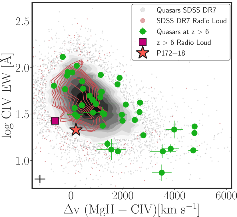
Figure 4: C IV  equivalent width vs. blueshift with respect to the Mg II  emission line. We show the distribution of SDSS DR7 $1.4<z<2.2$ quasars with gray points and shaded gray contours. The radio-loud subsample from SDSS is highlighted with red points and contours (see Section 3.1 for definition and selection). Quasars at $z>6$ are reported with green points, and obtained from a collection of works from the literature (Mazzucchelli et al. 2017, Shen et al. 2019, Onoue et al. 2020, Schindler et al. 2020). Before this work, there was only one $z>6$ radio-loud quasar with robust C IV and Mg II measurements (magenta square). P172+18 at $z=6.823$ is represented as an orange star and its uncertainties are shown in the bottom left corner.

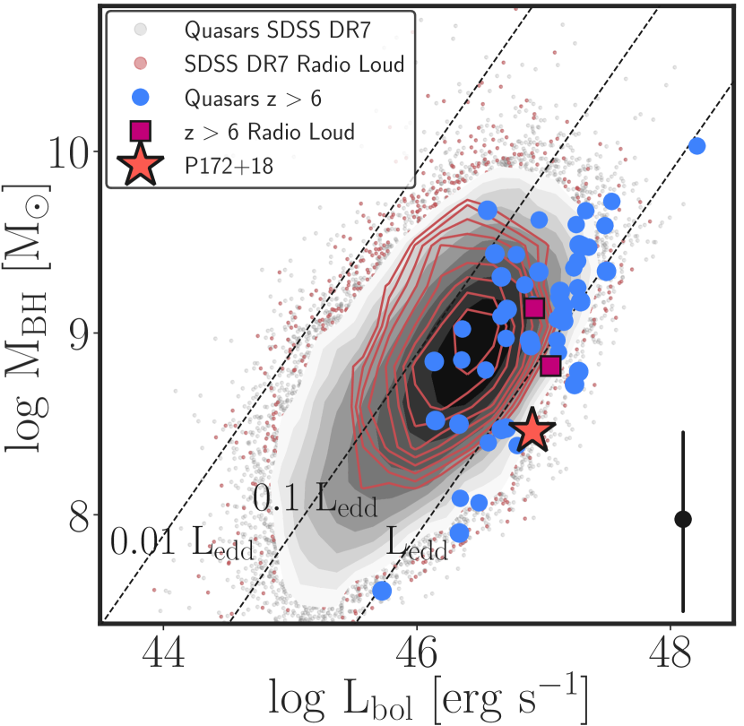
Figure 5: Black hole mass vs. bolometric luminosity. The gray points and contours show the distribution of SDSS DR7 quasars at $0.35<z<2.25$. Red points and contours highlight the SDSS DR7 radio-loud quasar subsample. We show $z>6$ radio-quiet and radio-loud quasars from a collection of studies in the literature (see Section 3.2 for references) with blue circles and magenta squares, respectively. P172+18 (orange star) is consistent with accreting matter at super-Eddington rate. The dominant systematic uncertainty on black hole mass estimates from scaling relations ($\sim$0.55 dex) is shown in the bottom right corner. All black hole masses shown here are estimated using the same scaling relation (Vestergaard & Osmer, 2009), and the same bolometric correction was applied for all bolometric luminosities (Richards et al., 2006).

3.3 Near-zone Size

Near-zones are regions around quasars where the surrounding intergalactic gas has been ionized by the quasar’s UV radiation, and they are observed as regions of enhanced transmitted flux close to the quasar in their rest-frame UV spectra. The near-zone sizes fo quasars provide constraints on quasar emission properties and on the state of their surrounding IGM (e.g., Fan et al. 2006, Eilers et al. 2017, 2018). The radii of near-zones ($R_{\rm NZ}$) depend on the rate of ionizing flux from the central source, on the quasar’s lifetime, and on the ionized fraction of the IGM (e.g., Fan et al. 2006, Davies et al. 2019). In practice, $R_{\rm NZ}$ is measured from the rest-frame UV spectrum (smoothed to a resolution of 20 Å) and taken to be the distance from the quasar at which the transmitted continuum-normalized flux drops below 10%. Here, we obtain the transmitted flux by dividing the observed spectrum of P172+18 by a model of the intrinsic continuum emission obtained with a principal components analysis method (see Davies et al. 2018; Eilers et al. 2020, for details of the method). In order to take into account the dependence on the quasar’s luminosity, we also calculate the corrected near-zone radius ($R_{\rm NZ,corr}$), following the scaling relation presented by Eilers et al. (2017):

$$R_{\rm NZ,corr}=R_{\rm NZ}\times 10^{0.4(27+M_{1450})/2.35}$$ (8)

where $M_{1450}$ is the absolute magnitude at rest-frame 1450 Å. We report both $R_{\rm NZ}$ and $R_{\rm NZ,corr}$ in Table 5. The size of the near-zone of P172+18 and the corrected near-zone are $R_{\rm NZ}=3.96\pm 0.48$ pMpc and $R_{\rm NZ,corr}=6.31\pm 0.76$ pMpc, respectively. This large near-zone is within the top quintile of the distribution of quasar near-zones at $z\gtrsim 6$ (Eilers et al., 2017). This suggests that the time during which this quasar is UV-luminous (here referred to its lifetime) exceeds the average lifetime of the high-redshift quasar population of $t_{\rm Q}\sim 10^{6}$ yr (Eilers et al., 2020).

The evolution of $R_{\rm NZ,corr}$ with redshift, at $z>5.5$, has been investigated in the literature to constrain both the reionization history and quasar lifetimes (e.g., Carilli et al. 2010, Davies et al. 2016, Eilers et al. 2020). While Carilli et al. (2010) and Venemans et al. (2015) recover a steep decline of $R_{\rm NZ,corr}$ with redshift (a decrease in size by a factor of $\sim 6$ between $z=6$ and $z=7$), Eilers et al. (2017) study a larger sample of $\sim$30 quasars at $5.8<z<6.6$ and recover a best-fit relation in the form of $R_{\rm NZ,corr}\propto(1+z)^{-\gamma}$, with $\gamma\sim 1.44$, suggesting a more moderate evolution with redshift than previous studies (a reduction in size by only $\sim 20\%$ between $z=6$ and $z=7$). Finally, Mazzucchelli et al. (2017) recover a flatter relation ($\gamma\sim 1.0$), utilizing measurements of $R_{\rm NZ,corr}$ up to $z\sim 7$ (see also Ishimoto et al. 2020). Using hydrodynamical simulations, Chen & Gnedin (2020) obtained a shallow redshift evolution of near-zone sizes over the redshift range probed by the current quasar sample, i.e., $5.5<z<7$ (see also Davies et al., 2020). The expected average corrected near-zone size at $z=6.8$ is $\langle R_{\rm NZ,corr}\rangle\approx 4.2$ pMpc for the redshift evolution from Eilers et al. (2017), and $\langle R_{\rm NZ,corr}\rangle\approx 2.2$ pMpc when assuming a steeper evolution as found by Venemans et al. (2015).

Therefore, the new near-zone measurement for P172+18 is considerably larger than the expected average size at this redshift. However, if the quasar was more luminous in the recent past and its activity is currently in a receding phase (see § 4.1 for tentative evidence of a decrease in the quasar’s radio luminosity), the large near-zone size could be explained by a higher luminosity than what is measured at the present time.

Table 1: Photometry of the radio-loud quasar P172+18 and its radio companion.

	Quasar	Radio Companion
R.A. (J2000)	$11^{\rm h}29^{\rm m}25\fs 37$	$11^{\rm h}29^{\rm m}24\fs 08$
Decl. (J2000)	$+18^{\circ}46^{\prime}24\farcs 29$	$+18^{\circ}46^{\prime}38\farcs 58$
Public optical and infrared surveys
Pan-STARRS1 $i_{\rm P1}$	$>23.6$	$>23.6$
Pan-STARRS1 $z_{\rm P1}$	$>23.2$	$>23.2$
Pan-STARRS1 $y_{\rm P1}$	$20.76\pm 0.09$	$>22.3$
DECaLS DR8 $g_{\rm DE}$	$>25.4$	$>25.4$
DECaLS DR8 $r_{\rm DE}$	$>24.8$	$>24.8$
DECaLS DR8 $z_{\rm DE}$	$21.64\pm 0.05$	$>23.8$
DECaLS DR8 $W1$	$20.71\pm 0.13$	$>21.8$
DECaLS DR8 $W2$	$20.73\pm 0.31$	$>20.9$
Follow-up near-infrared imaging
$J_{\rm NOT}$	$20.90\pm 0.11$	$>22.2$
$H_{\rm NOT}$	$21.36\pm 0.24$	$>21.8$
$Ks_{\rm NOT}$	$21.07\pm 0.18$	$>21.7$
Public radio surveys
TGSS 147.5 MHz	$<8.5\,\mathrm{mJy}$	$<8.5\,\mathrm{mJy}$
FIRST 1.4 GHz	$1020\pm 144\,\mu\mathrm{Jy}$	$<406\,\mu\mathrm{Jy}$
Radio follow-up
VLA-L $1.52\,$GHz	$510\pm 15\,\mu\mathrm{Jy}$	$732\pm 15\,\mu\mathrm{Jy}$
VLA-S $2.87\,$GHz	$222\pm 9\,\mu\mathrm{Jy}$	$432\pm 20\,\mu\mathrm{Jy}$
$\alpha_{S}^{L}$	$-1.31\pm 0.08$	$-0.83\pm 0.08$
Quasar rest-frame luminosities
$m_{1450}$	$21.08\pm 0.10$
$M_{1450}$	$-25.81\pm 0.10$
$L_{2500}$	$(1.4\pm 0.1)\times 10^{46}\,$erg s-1
$L_{3000}$	$(1.3\pm 0.1)\times 10^{46}$ erg s-1
$L_{4400}$	$(1.1\pm 0.1)\times 10^{46}\,$erg s-1
$L_{5\,\mathrm{GHz}}$	$(5.4\pm 0.2)\times 10^{42}\,$erg s-1

4 Analysis of Radio Properties

In addition to detecting the quasar, the follow-up VLA radio observations revealed a second radio source 23$\farcs$1 from P172+18 at a position angle of $128.25^{\circ}$ (see Figure 3). We will explore the radio properties of the quasar and the serendipitous companion radio source below.

4.1 Quasar Radio Properties

The quasar is a point source in both the follow-up L- and S-band observations with a deconvolved size smaller than $1\farcs 9\times 0\farcs 87$; see Figure 3. P172+18 is well detected in both bands with S/N $>20$ and the measured flux densities are listed in Table 1. The measured L-band flux density is a factor of two fainter than what is reported in the FIRST catalog. In fact, the measured $f_{1.52\,\mathrm{GHz}}=510\pm 15\,\mu$Jy would have been below the detection threshold of the FIRST survey (Becker et al., 1995). The discrepancy is significant at more than $3\sigma$ and could be the result of real quasar variability over the 20 yr ($\sim 2.5$ yr rest frame) between the two measurements; such changes have been reported in similar timescales (e.g., Nyland et al., 2020). However, given that the source is at the faint limit of the FIRST survey, we cannot rule out that the variation is simply due to noise fluctuations in the FIRST data. Unfortunately, we are not able to test the variability hypothesis given that no other measurements of the quasar are available at a similar epoch to the FIRST observation. For the remainder of the analysis we will consider the follow-up VLA measurements as the true fluxes. Assuming that the radio observations follow a power-law spectral energy distribution ($f_{\nu}\propto\nu^{\alpha}$), the L- and S-band flux densities correspond to a steep power-law radio slope of $\alpha_{S}^{L}=-1.31\pm 0.08$. This is steeper than $\alpha=-0.75$, which is usually assumed in high-redshift quasar studies when only one radio band is available (e.g., Wang et al. 2007; Momjian et al. 2014; Bañados et al. 2015).

4.1.1 Radio-loudness

To estimate the radio-loudness of P172+18 we obtain the rest-frame 5 GHz emission by extrapolating the radio emission using the measured spectral index $\alpha_{S}^{L}=-1.31$ and the 2500 Å and 4400 Å emission using the power-law fit to the near-infrared spectrum ($\alpha_{\nu,\mathrm{UV}}=-0.48$) obtained in Section 3. This results in radio-loudness parameters of $R_{2500}=91\pm 9$ and $R_{4400}=70\pm 7$, classifying P172+18 as a radio-loud quasar. The quasar radio properties are summarized in Table 5.

We note that the data from very long baseline interferometry (VLBI) presented by Momjian et al. (2021) imply a steeper spectral index at frequencies higher than 3 GHz (see Figure 6). The quasar is not detected in the TIFR GMRT Sky Survey (TGSS; Intema et al., 2017) at 147.5 MHz. We downloaded the TGSS image and determined a $3\sigma$ upper limit of 8.5 mJy (see Table 1 and Figure 6). This implies that the slope of the radio spectrum should flatten or have a turnover between 147.5 MHz and 1.52 GHz. If the turnover occurs at a frequency larger than rest-frame 5 GHz, the rest-frame 5 GHz luminosity (and therefore radio-loudness) would be smaller than our fiducial value assuming $\alpha=-1.31$. In the extreme case that the turnover happened exactly at the frequency of our L-band observations, the source would still be classified as radio-loud (i.e., $R_{2500}>10$) as long as $\alpha<1.24$ (see Figure 6). Deep radio observations at frequencies $<1$ GHz are needed to precisely determine the rest-frame 5 GHz luminosity and the shape of the radio spectrum.

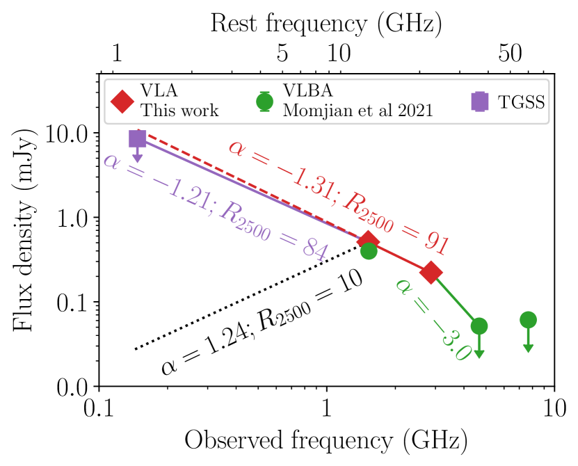
Figure 6: Radio spectral energy distribution of P172+18, including data from our VLA follow-up observations (red diamond), the VLBI measurements (green circles) from Momjian et al. (2021), and a $3\sigma$ upper limit from the TGSS (purple square). The power-law index, $\alpha$, is shown between the measurements as well as the radio-loudness by extrapolating the radio emission to rest-frame 5GHz. The dotted line with $\alpha=1.24$ represents the turnover required for P172+18 to be classified as radio-quiet (i.e., $R_{2500}<10$).

4.2 Companion Radio Source

The radio companion is detected with S/N $>$ $20$ in both L- and S-band observations (see Figure 3). This object is a point source in the L-band image with a deconvolved size smaller than $1\farcs 6\times 0\farcs 69$. A Gaussian fit to the S-band image results in a resolved source with a deconvolved size of $1\farcs 3\times 0\farcs 8$ and position angle of $74^{\circ}\pm 22^{\circ}$. This secondary source is not detected in any of our available optical, near-infrared, and mid-infrared images. Its radio properties and optical/near-infrared limits are listed in Table 1.

The number of radio sources with a 1.4 GHz flux density $>700\,\mu$Jy is 59 deg^-2 and 117 deg^-2 according to the number counts of deep radio surveys from Fomalont et al. (2006) and Bondi et al. (2008), respectively. This means that in an area encompassing the quasar and the second radio source ($\pi\times 23\farcs 1^{2}$) only 0.007 and 0.015 sources like the companion are expected using the number counts from Fomalont et al. (2006) and Bondi et al. (2008), respectively. The $<2\%$ likelihood of chance superposition raises the possibility that this radio source and the quasar could be associated.

This companion radio source is (slightly) brighter than the quasar in both the L- and S-band follow-up observations. However, it was not detected in the FIRST survey carried out in 1999 (see Table 1 and Figure 3). This second source could not be a hot spot of the radio jet expanding for the last 20 yr: at the redshift of the quasar, the projected separation of the two sources is about 120 proper kpc, a distance that would take light about $400,000$ yr to travel.

Another possibility is that this second source is an obscured, radio-AGN companion. There are a few examples of associated dust-obscured, star-forming companion galaxies to quasars at $z>6$ (e.g., Decarli et al., 2017; Neeleman et al., 2019). A couple of them have tentative X-ray detections, which make them obscured AGN candidates (e.g., Connor et al., 2019; Vito et al., 2019). This possibility is tempting, because two associated radio-loud AGNs would point to an overdense environment in the early universe and provide constraints on AGN clustering. Nevertheless, with the available shallow optical and near-infrared data we are not able to rule out that the second radio source lies at a different redshift than that of the quasar. More follow-up observations are required to firmly establish the nature and redshift of the source.

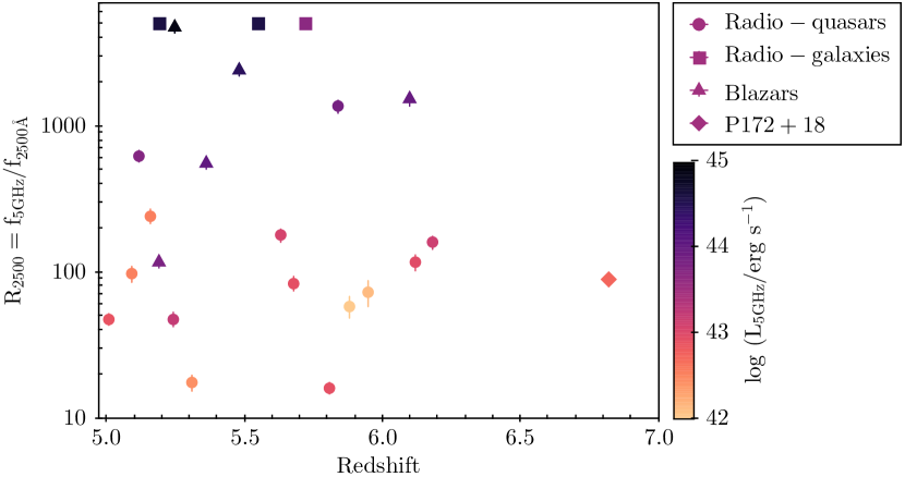
Figure 7: All radio-loud ($R_{2500}>10$) sources known at $z>5$, color-coded by their rest-frame 5 GHz radio luminosity. Radio-loud quasars are shown as circles and radio galaxies as squares. The radio-loudness for radio galaxies has been fixed to 5000 for visualization purposes. The properties and references for all these sources are listed in Table 5.

5 Summary and conclusions

The main results of this work can be summarized as follows.

1. We present the discovery of the most distant radio-loud source to date, the quasar P172+18 with an Mg II-based redshift of $z=6.823$ (see Figures 1 and 7 and Table 5).

2. The C IV properties of the two $z>6$ radio-loud quasars known with near-infrared spectroscopy and reliable C IV detection (J1427+5447 and P172+18) are consistent with the radio-loud population at $z\sim 2$ in terms of C IV EW and blueshift (see Figure 4).

3. The quasar has a black hole mass of $\sim 2.9\times 10^{8}M_{\odot}$ and an Eddington ratio of $\sim$2.2. It is known that there are large uncertainties on the estimates of black hole mass and Eddington ratio associated with the scaling relations used. Therefore we compare the properties of P172+18 to other quasars using the same scaling relation (Vestergaard & Osmer, 2009) and bolometric correction (Richards et al., 2006). With this in mind, P172+18 is among the fastest accreting quasars at both low and high redshift (Figure 5).

4. The quasar shows a strong $\mathrm{Ly}\alpha$ line that can be modeled with a narrow Gaussian and a broad one (see Figure 2 and Table 3). The large measured near-zone size, $R_{\rm NZ,corr}\sim 6$ pMpc, suggests an ionized IGM around the quasar and implies that P172+18’s lifetime exceeds the average lifetime of the $z\gtrsim 6$ quasar population (see Section 3.3).

5. The quasar’s radio emission is unresolved (with size smaller than $1\farcs 90\times 0\farcs 87$) and shows a steep radio spectrum ($\alpha=-1.31\pm 0.08$) between 1.5 and 3.0 GHz ($\sim$11–23 GHz in the rest frame). Extrapolating the spectrum to 5 GHz rest frame, the quasar has a radio-loudness of $R_{2500}=91\pm 9$ (see Figure 6).

6. The follow-up L-band radio data are a factor $\sim 2$ fainter than what is expected from the FIRST observations taken two decades previously. This fact, together with the long lifetime implied by the size of P172+18’s near-zone, could indicate that we are witnessing the quasar phase turning off.

7. The VLA follow-up observations revealed a second radio source 23$\farcs$1 from the quasar with comparable radio flux densities (see Figure 3 and Table 1). This source was not detected in the FIRST survey and has no counterpart in our current optical/near-infrared images.

P172+18, in particular, is an ideal target to investigate the existence of extended X-ray emission arising from the interaction between relativistic particles in radio jets and a hot cosmic microwave background (CMB) (e.g., Wu et al., 2017). This effect is expected to be particularly strong at the highest redshifts because the CMB energy density scales as $(1+z)^{4}$ and as a result its effective magnetic field can be stronger than the one in radio-lobes (Ghisellini et al., 2015). Complementary to this science case will be high-resolution VLBI observations to constrain the structure of the radio emission (e.g., Frey et al., 2008; Momjian et al., 2008, 2018). VLBI observations for P172+18 already exist and the results will be presented in the companion paper by Momjian et al. (2021).

The serendipitous detection of the companion radio source (see Figure 3) deserves further follow-up. If the radio source lies at the same redshift as the quasar, this could be the most distant AGN pair known, potentially revealing a very dense region in the early universe. Telescopes such as the Atacama Large Millimeter/submillimeter Array or the James Webb Space Telescope should be able to determine the exact redshift by identifying far-infrared and optical emission lines from this possible obscured AGN.

Out of the 18 quasars known at $z>6.8$, P172+18 is the only one currently classified as radio-loud. In Table 5 we compile the information on all the radio-loud sources at $z>5$ known to date and in Figure 7 we present their redshift and radio-loudness distribution. The radio-loudness of P172+18 is consistent with the median value of the $z>5$ radio-loud quasar population ($R_{2500,\mathrm{median}}=91$; $R_{2500,\mathrm{mean}}=213$). Thus, the existence of this “median” radio-loud quasar at $z=6.823$ makes it likely that there are other radio-loud sources waiting to be discovered (or categorized) between this redshift and the previous redshift record, and possibly even at $z>7$. Identifying these radio sources would be important for future 21cm absorption studies of the IGM with the Square Kilometre Array (Carilli et al., 2004; Carilli & Rawlings, 2004; Ciardi et al., 2015).

Table 2: Observing Log of Optical and Radio Imaging

Date	Telescope/Instrument	Filters/frequency	rms ($1\sigma$)	Reference
2019 May 17	NOT/NOTCAM	$J_{\rm NOT}$,$H_{\rm NOT}$	23.4, 23.0 mag	This work
2019 May 18	NOT/NOTCAM	$Ks_{\rm NOT}$	22.9 mag	This work
1999 Nov 10	VLA/L-band	1.44 GHz	135 $\mu$Jy	FIRST
2019 Mar 5	VLA/S-band	2.87 GHz	9 $\mu$Jy	This work
2019 Mar 11	VLA/L-band	1.58 GHz	15 $\mu$Jy	This work

Table 3: Summary of the optical and near-infrared follow-up spectroscopic observations.

Date	Telescope/Instrument	Exposure Time	Wavelength Range	Slit Width
2019 Feb 18	Keck/NIRES	3.5 hr	9400$-$24000 Å	0$\farcs$55
2019 Mar 8$-$Apr 8	VLT/X-Shooter	3.5 hr	3000$-$24800 Å	1$\farcs$0 / 0$\farcs$9 / 0$\farcs$6
2019 Jun 13	LBT/MODS	0.3 hr	5000$-$10000 Å	1$\farcs$22

Table 4: Properties of P172+18 measured from near-infrared spectroscopy.

Emission Line	Redshift	FWHM	EW	$\rm\Delta$vMgII-line
		(km s-1)	($\rm\AA$)	(km s-1)
$\mathrm{Ly}\alpha$  (1)	6.8234$\pm$0.0002	891${}^{+27}_{-25}$	–	$-$15$\pm$77
$\mathrm{Ly}\alpha$  (2)	6.854$\pm$0.001	2870${}^{+91}_{-77}$	–	$-$304$\pm$88
$\mathrm{Ly}\alpha$	6.8246$\pm$0.0008	1103${}^{+27}_{-22}$	38.1$\pm$1.8	$-$60$\pm$83
N V	6.817$\pm$0.001	3076${}^{+0.3}_{-0.1}$	18.1$\pm$1.1	215$\pm$91
$\mathrm{Ly}\alpha$ + N V	–	–	56.3$\pm$3.0	–
Si IV+ [O IV]	6.822$\pm$0.05	3044${}^{+1104}_{-652}$	8.6${}^{+1.7}_{-1.4}$	38$\pm$1918
C IV  (1)	6.819${}^{+0.004}_{-0.007}$	1699${}^{+840}_{-499}$	–	153$\pm$224
C IV  (2)	6.753${}^{+0.02}_{-0.03}$	5001${}^{+1018}_{-2143}$	–	2682$\pm$961
C IV	6.818${}^{+0.004}_{-0.006}$	2714${}^{+1704}_{-945}$	21.3${}^{+2.4}_{-2.0}$	192$\pm$225
C III]	6.799${}^{+0.008}_{-0.005}$	5073${}^{+560}_{-461}$	28.9${}^{+3.4}_{-3.3}$	920$\pm$260
Mg II	6.823${}^{+0.003}_{-0.001}$	1780${}^{+100}_{-50}$	20.8${}^{+2.8}_{-2.6}$	–
Power-law slope ($\alpha_{\lambda,\mathrm{UV}}$)	–1.52 $\pm$ 0.05
Power-law ampl. ($f_{\lambda,2500\mathrm{,obs}}$)	1.36 $\pm$ 0.03 [$\times$ 10-18 erg s-1 cm-2 Å-1]

The redshift of P172+18 used throughout the paper is taken from the fit to the Mg II emission line, as reported here.

Table 5: P172+18 properties derived from the optical and near-infrared spectroscopy and radio observations.

Quantity
$L_{\mathrm{bol}}$	(8.1 $\pm 0.3)\times 10^{46}$ erg s-1
$M_{\mathrm{BH}}$	2.9${}^{+0.7}_{-0.6}\times 10^{8}$ $M_{\odot}$
$L_{\mathrm{bol}}$/$L_{\mathrm{Edd}}$	2.2${}^{+0.6}_{-0.4}$
Fe II/Mg II	2.8$\pm$1.0
$R_{\rm NZ}$	$3.96\pm 0.48~{}\rm pMpc$
$R_{\rm NZ,corr}$	$6.31\pm 0.76~{}\rm pMpc$
$R_{2500}$	$91\pm 9$
$R_{4400}$	$70\pm 7$

Table 6: Census and Properties of $z>5$ Radio-loud Sources, Sorted by Decreasing Redshift, $z$

Name	$z$	Type	$m_{1450}$	$\alpha_{\lambda,\mathrm{UV}}$	$f_{1.4\,\mathrm{GHz}}$	$\alpha_{\nu,\mathrm{radio}}$	$R_{2500}$	References
			(mag)		(mJy)			disc./$z$/$m_{1450}$/$\alpha_{\lambda,\mathrm{UV}}$/$f_{1.4\,\mathrm{GHz}}$/$\alpha_{\nu,\mathrm{radio}}$
P172+18	6.823	quasar	21.08	$-1.52$	$0.510\pm 0.016$	$-1.31$	$91\pm 9$	1/1/1/1/1/1
J1429+5447	6.183	quasar	20.70	$-1.22$	$2.93\pm 0.15$	$-0.67$	$161\pm 17$	2/3/4/–/5/6
J1427+3312	6.121	quasar	20.68	–	$1.73\pm 0.13$	$-0.90$	$117\pm 14$	7,8/9/4/–/5/6
J0309+27172	6.10	blazar	20.96	–	$23.89\pm 0.87$	$-0.44$	$1521\pm 151$	10/10/11/–/12/10
J2228+0110	5.95	quasar	22.20	–	$0.31\pm 0.06$	–	$71\pm 15$	13/13/13/–/13/–
J2242+0334	5.88	quasar	22.20	–	$0.20\pm 0.03$	$-1.06$	$58\pm 9$	2/2/4/–/14/14
P352–15	5.84	quasar	21.05	–	$14.9\pm 0.70$	$-0.89$	$1358\pm 141$	15/15/15/–/12/15
J0836+0054	5.81	quasar	18.95	$-0.73$	$1.74\pm 0.04$	$-0.86$	$16\pm 1$	16/17/4/9/18/6
J1530+1049	5.72	radio galaxy	–	–	$7.50\pm 0.10$	$-1.40$	–	19/19/–/–/19/19
P055–00	5.68	quasar	20.29	–	$2.14\pm 0.14$	–	$83\pm 9$	20/20/4/–/5/–
P135+16	5.63	quasar	20.74	–	$3.04\pm 0.15$	–	$177\pm 18$	20/20/4/–/5/–
J0856+0223	5.55	radio galaxy	–	–	$86.50\pm 0.60$	$-0.89$	–	21/21/–/–/21/21
J0906+6930	5.48	blazar	19.67	$-2.00$	$92.0\pm 0.62$	$-0.40$	$2373\pm 205$	22/23/11/23/22/22
J1648+4603	5.36	blazar	19.51	–	$34.0\pm 0.01$	$-0.47$	$552\pm 47$	24/24/11/–/24/24
J1614+4650	5.31	quasar	19.72	–	$1.69\pm 0.16$	$0.67$	$17\pm 2$	24/25/11/–/5/6
J1026+2542	5.25	blazar	19.69	–	$230.00\pm 0.14$	$-0.60$	$4701\pm 407$	24/25/11/–/5/26
J2329+3003	5.24	quasar	18.83	–	$4.90\pm 0.40$	–	$47\pm 5$	27/28/27/–/12/–
J0924–2201	5.19	radio galaxy	–	–	$71.10\pm 0.10$	$-1.63$	–	29/29/–/–/29/29
J0131–0321	5.189	blazar	18.09	$-1.75$	$32.83\pm 0.12$	$0.29$	$116\pm 9$	30/30/30/30/5/6
J2245+0024	5.16	quasar	22.24	–	$1.09\pm 0.06$	–	$240\pm 27$	31/31/31/–/32/–
J0913+5919	5.12	quasar	20.26	–	$17.45\pm 0.16$	$-0.67$	$618\pm 55$	24/25/11/–/5/33
J2239+0030	5.09	quasar	21.27	–	$1.35\pm 0.10$	$-0.27$	$98\pm 12$	31/31/31/–/5/6
J1034+2033	5.01	quasar	19.56	–	$3.96\pm 0.15$	$0.28$	$47\pm 4$	24/25/11/–/5/6

Note. — Blazars are highly variable objects and the UV and radio properties for the objects in this list were not observed simultaneously. Therefore, the radio-loudness reported here should be treated with caution, especially for blazars.

References. — 1: This work; 2: Willott et al. (2010a); 3: Wang et al. (2011); 4: Bañados et al. (2016); 5: Becker et al. (1995); 6: Shao et al. (2020); 7: McGreer et al. (2006); 8: Stern et al. (2007); 9: Shen et al. (2019); 10: Belladitta et al. (2020); 11: $y_{\rm P1}$ magnitude; 12: Condon et al. (1998); 13: Zeimann et al. (2011); 14: Liu et al. (2021); 15: Bañados et al. (2018a); 16: Fan et al. (2001); 17: Kurk et al. (2007); 18: Wang et al. (2007); 19: Saxena et al. (2018); 20: Bañados et al. (2015); 21: Drouart et al. (2020); 22: Romani et al. (2004); 23: An & Romani (2018); 24: Schneider et al. (2010); 25: Pâris et al. (2018); 26: Frey et al. (2015); 27: Wang et al. (2016); 28: Yang et al. (2016); 29: van Breugel et al. (1999); 30: Yi et al. (2014); 31: McGreer et al. (2013); 32: Hodge et al. (2011); 33: Wu et al. (2013)

References

- An & Romani (2018) An, H., & Romani, R. W. 2018, ApJ, 856, 105, doi: 10.3847/1538-4357/aab435
- Andika et al. (2020) Andika, I. T., Jahnke, K., Onoue, M., et al. 2020, ApJ, 903, 34, doi: 10.3847/1538-4357/abb9a6
- Astropy Collaboration et al. (2018) Astropy Collaboration, Price-Whelan, A. M., Sipőcz, B. M., et al. 2018, AJ, 156, 123, doi: 10.3847/1538-3881/aabc4f
- Bañados et al. (2018a) Bañados, E., Carilli, C., Walter, F., et al. 2018a, ApJ, 861, L14, doi: 10.3847/2041-8213/aac511
- Bañados et al. (2014) Bañados, E., Venemans, B. P., Morganson, E., et al. 2014, AJ, 148, 14, doi: 10.1088/0004-6256/148/1/14
- Bañados et al. (2015) —. 2015, ApJ, 804, 118, doi: 10.1088/0004-637X/804/2/118
- Bañados et al. (2016) Bañados, E., Venemans, B. P., Decarli, R., et al. 2016, ApJS, 227, 11, doi: 10.3847/0067-0049/227/1/11
- Bañados et al. (2018b) Bañados, E., Venemans, B. P., Mazzucchelli, C., et al. 2018b, Nature, 553, 473, doi: 10.1038/nature25180
- Becker et al. (1995) Becker, R. H., White, R. L., & Helfand, D. J. 1995, ApJ, 450, 559, doi: 10.1086/176166
- Belladitta et al. (2020) Belladitta, S., Moretti, A., Caccianiga, A., et al. 2020, A&A, 635, L7, doi: 10.1051/0004-6361/201937395
- Bondi et al. (2008) Bondi, M., Ciliegi, P., Schinnerer, E., et al. 2008, ApJ, 681, 1129, doi: 10.1086/589324
- Carilli et al. (2004) Carilli, C. L., Furlanetto, S., Briggs, F., et al. 2004, NewAR, 48, 1029, doi: 10.1016/j.newar.2004.09.046
- Carilli et al. (2002) Carilli, C. L., Gnedin, N. Y., & Owen, F. 2002, ApJ, 577, 22, doi: 10.1086/342179
- Carilli & Rawlings (2004) Carilli, C. L., & Rawlings, S. 2004, New A Rev., 48, 979, doi: 10.1016/j.newar.2004.09.001
- Carilli et al. (2010) Carilli, C. L., Wang, R., Fan, X., et al. 2010, ApJ, 714, 834, doi: 10.1088/0004-637X/714/1/834
- Chambers et al. (2016) Chambers, K. C., Magnier, E. A., Metcalfe, N., et al. 2016, ArXiv e-prints. https://arxiv.org/abs/1612.05560
- Chen & Gnedin (2020) Chen, H., & Gnedin, N. Y. 2020, arXiv e-prints, arXiv:2008.04911. https://arxiv.org/abs/2008.04911
- Ciardi et al. (2015) Ciardi, B., Inoue, S., Mack, K., Xu, Y., & Bernardi, G. 2015, in Advancing Astrophysics with the Square Kilometre Array (AASKA14), 6. https://arxiv.org/abs/1501.04425
- Ciardi et al. (2013) Ciardi, B., Labropoulos, P., Maselli, A., et al. 2013, MNRAS, 428, 1755, doi: 10.1093/mnras/sts156
- Clough et al. (2005) Clough, S. A., Shephard, M. W., Mlawer, E. J., et al. 2005, J. Quant. Spec. Radiat. Transf., 91, 233, doi: 10.1016/j.jqsrt.2004.05.058
- Condon et al. (1998) Condon, J. J., Cotton, W. D., Greisen, E. W., et al. 1998, AJ, 115, 1693, doi: 10.1086/300337
- Connor et al. (2019) Connor, T., Bañados, E., Stern, D., et al. 2019, ApJ, 887, 171, doi: 10.3847/1538-4357/ab5585
- Cutri (2014) Cutri, R. M., e. 2014, VizieR Online Data Catalog, 2328, 0
- Davies et al. (2016) Davies, F. B., Furlanetto, S. R., & McQuinn, M. 2016, MNRAS, 457, 3006, doi: 10.1093/mnras/stw055
- Davies et al. (2019) Davies, F. B., Hennawi, J. F., & Eilers, A.-C. 2019, ApJ, 884, L19, doi: 10.3847/2041-8213/ab42e3
- Davies et al. (2020) —. 2020, MNRAS, 493, 1330, doi: 10.1093/mnras/stz3303
- Davies et al. (2018) Davies, F. B., Hennawi, J. F., Bañados, E., et al. 2018, ApJ, 864, 143, doi: 10.3847/1538-4357/aad7f8
- De Rosa et al. (2011) De Rosa, G., Decarli, R., Walter, F., et al. 2011, ApJ, 739, 56, doi: 10.1088/0004-637X/739/2/56
- Decarli et al. (2017) Decarli, R., Walter, F., Venemans, B. P., et al. 2017, Nature, 545, 457, doi: 10.1038/nature22358
- Dey et al. (2019) Dey, A., Schlegel, D. J., Lang, D., et al. 2019, AJ, 157, 168, doi: 10.3847/1538-3881/ab089d
- Diamond-Stanic et al. (2009) Diamond-Stanic, A. M., Fan, X., Brandt, W. N., et al. 2009, ApJ, 699, 782, doi: 10.1088/0004-637X/699/1/782
- Dietrich et al. (2003) Dietrich, M., Hamann, F., Appenzeller, I., & Vestergaard, M. 2003, ApJ, 596, 817, doi: 10.1086/378045
- Djupvik & Andersen (2010) Djupvik, A. A., & Andersen, J. 2010, Astrophysics and Space Science Proceedings, 14, 211, doi: 10.1007/978-3-642-11250-8_21
- Drouart et al. (2020) Drouart, G., Seymour, N., Galvin, T. J., et al. 2020, PASA, 37, e026, doi: 10.1017/pasa.2020.6
- Eilers et al. (2018) Eilers, A.-C., Davies, F. B., & Hennawi, J. F. 2018, ApJ, 864, 53, doi: 10.3847/1538-4357/aad4fd
- Eilers et al. (2017) Eilers, A.-C., Davies, F. B., Hennawi, J. F., et al. 2017, ApJ, 840, 24, doi: 10.3847/1538-4357/aa6c60
- Eilers et al. (2020) Eilers, A.-C., Hennawi, J. F., Decarli, R., et al. 2020, ApJ, 900, 37, doi: 10.3847/1538-4357/aba52e
- Eisenhardt et al. (2020) Eisenhardt, P. R. M., Marocco, F., Fowler, J. W., et al. 2020, ApJS, 247, 69, doi: 10.3847/1538-4365/ab7f2a
- Fan et al. (2001) Fan, X., Narayanan, V. K., Lupton, R. H., et al. 2001, AJ, 122, 2833, doi: 10.1086/324111
- Fan et al. (2006) Fan, X., Strauss, M. A., Richards, G. T., et al. 2006, AJ, 131, 1203, doi: 10.1086/500296
- Fomalont et al. (2006) Fomalont, E. B., Kellermann, K. I., Cowie, L. L., et al. 2006, ApJS, 167, 103, doi: 10.1086/508169
- Frey et al. (2008) Frey, S., Gurvits, L. I., Paragi, Z., & É. Gabányi, K. 2008, A&A, 484, L39, doi: 10.1051/0004-6361:200810040
- Frey et al. (2015) Frey, S., Paragi, Z., Fogasy, J. O., & Gurvits, L. I. 2015, MNRAS, 446, 2921, doi: 10.1093/mnras/stu2294
- Ghisellini et al. (2015) Ghisellini, G., Haardt, F., Ciardi, B., et al. 2015, MNRAS, 452, 3457, doi: 10.1093/mnras/stv1541
- Gullikson et al. (2014) Gullikson, K., Dodson-Robinson, S., & Kraus, A. 2014, AJ, 148, 53, doi: 10.1088/0004-6256/148/3/53
- Hardcastle & Croston (2020) Hardcastle, M. J., & Croston, J. H. 2020, New A Rev., 88, 101539, doi: 10.1016/j.newar.2020.101539
- Harris et al. (2020) Harris, C. R., Millman, K. J., van der Walt, S. J., et al. 2020, Nature, 585, 357, doi: 10.1038/s41586-020-2649-2
- Hodge et al. (2011) Hodge, J. A., Becker, R. H., White, R. L., Richards, G. T., & Zeimann, G. R. 2011, AJ, 142, 3, doi: 10.1088/0004-6256/142/1/3
- Horne (1986) Horne, K. 1986, PASP, 98, 609, doi: 10.1086/131801
- Hunter (2007) Hunter, J. D. 2007, Computing in Science and Engineering, 9, 90, doi: 10.1109/MCSE.2007.55
- Intema et al. (2017) Intema, H. T., Jagannathan, P., Mooley, K. P., & Frail, D. A. 2017, A&A, 598, A78, doi: 10.1051/0004-6361/201628536
- Ishimoto et al. (2020) Ishimoto, R., Kashikawa, N., Onoue, M., et al. 2020, ApJ, 903, 60, doi: 10.3847/1538-4357/abb80b
- Jiang et al. (2007) Jiang, L., Fan, X., Ivezić, Ž., et al. 2007, ApJ, 656, 680, doi: 10.1086/510831
- Jolley & Kuncic (2008) Jolley, E. J. D., & Kuncic, Z. 2008, MNRAS, 386, 989, doi: 10.1111/j.1365-2966.2008.13082.x
- Kellermann et al. (1989) Kellermann, K. I., Sramek, R., Schmidt, M., Shaffer, D. B., & Green, R. 1989, AJ, 98, 1195, doi: 10.1086/115207
- Kratzer & Richards (2015) Kratzer, R. M., & Richards, G. T. 2015, AJ, 149, 61, doi: 10.1088/0004-6256/149/2/61
- Kurk et al. (2007) Kurk, J. D., Walter, F., Fan, X., et al. 2007, ApJ, 669, 32, doi: 10.1086/521596
- Lang (2014) Lang, D. 2014, AJ, 147, 108, doi: 10.1088/0004-6256/147/5/108
- Leighly & Moore (2004) Leighly, K. M., & Moore, J. R. 2004, ApJ, 611, 107, doi: 10.1086/422088
- Liu et al. (2021) Liu, Y., Wang, R., Momjian, E., et al. 2021, ApJ, 908, 124, doi: 10.3847/1538-4357/abd3a8
- Matsuoka et al. (2019a) Matsuoka, Y., Iwasawa, K., Onoue, M., et al. 2019a, ApJ, 883, 183, doi: 10.3847/1538-4357/ab3c60
- Matsuoka et al. (2019b) Matsuoka, Y., Onoue, M., Kashikawa, N., et al. 2019b, ApJ, 872, L2, doi: 10.3847/2041-8213/ab0216
- Mazzucchelli et al. (2017) Mazzucchelli, C., Bañados, E., Venemans, B. P., et al. 2017, ApJ, 849, 91, doi: 10.3847/1538-4357/aa9185
- McGreer et al. (2006) McGreer, I. D., Becker, R. H., Helfand, D. J., & White, R. L. 2006, ApJ, 652, 157, doi: 10.1086/507767
- McGreer et al. (2013) McGreer, I. D., Jiang, L., Fan, X., et al. 2013, ApJ, 768, 105, doi: 10.1088/0004-637X/768/2/105
- McMullin et al. (2007) McMullin, J. P., Waters, B., Schiebel, D., Young, W., & Golap, K. 2007, in Astronomical Society of the Pacific Conference Series, Vol. 376, Astronomical Data Analysis Software and Systems XVI, ed. R. A. Shaw, F. Hill, & D. J. Bell, 127
- Meisner et al. (2019) Meisner, A. M., Lang, D., Schlafly, E. F., & Schlegel, D. J. 2019, PASP, 131, 124504, doi: 10.1088/1538-3873/ab3df4
- Meisner et al. (2017) Meisner, A. M., Lang, D., & Schlegel, D. J. 2017, AJ, 154, 161, doi: 10.3847/1538-3881/aa894e
- Meyer et al. (2019) Meyer, R. A., Bosman, S. E. I., & Ellis, R. S. 2019, MNRAS, 487, 3305, doi: 10.1093/mnras/stz1504
- Momjian et al. (2021) Momjian, E., Bañados, E., Carilli, C. L., et al. 2021, AJ in press
- Momjian et al. (2018) Momjian, E., Carilli, C. L., Bañados, E., Walter, F., & Venemans, B. P. 2018, ApJ, 861, 86, doi: 10.3847/1538-4357/aac76f
- Momjian et al. (2008) Momjian, E., Carilli, C. L., & McGreer, I. D. 2008, AJ, 136, 344, doi: 10.1088/0004-6256/136/1/344
- Momjian et al. (2014) Momjian, E., Carilli, C. L., Walter, F., & Venemans, B. 2014, AJ, 147, 6, doi: 10.1088/0004-6256/147/1/6
- Neeleman et al. (2019) Neeleman, M., Bañados, E., Walter, F., et al. 2019, ApJ, 882, 10, doi: 10.3847/1538-4357/ab2ed3
- Noirot et al. (2018) Noirot, G., Stern, D., Mei, S., et al. 2018, ApJ, 859, 38, doi: 10.3847/1538-4357/aabadb
- Nyland et al. (2020) Nyland, K., Dong, D. Z., Patil, P., et al. 2020, ApJ, 905, 74, doi: 10.3847/1538-4357/abc341
- Oesch et al. (2014) Oesch, P. A., Bouwens, R. J., Illingworth, G. D., et al. 2014, ApJ, 786, 108, doi: 10.1088/0004-637X/786/2/108
- Onoue et al. (2019) Onoue, M., Kashikawa, N., Matsuoka, Y., et al. 2019, ApJ, 880, 77, doi: 10.3847/1538-4357/ab29e9
- Onoue et al. (2020) Onoue, M., Bañados, E., Mazzucchelli, C., et al. 2020, ApJ, 898, 105, doi: 10.3847/1538-4357/aba193
- Overzier (2016) Overzier, R. A. 2016, A&A Rev., 24, 14, doi: 10.1007/s00159-016-0100-3
- Padovani (2017) Padovani, P. 2017, Nature Astronomy, 1, 0194, doi: 10.1038/s41550-017-0194
- Pâris et al. (2018) Pâris, I., Petitjean, P., Aubourg, É., et al. 2018, A&A, 613, A51, doi: 10.1051/0004-6361/201732445
- Pogge et al. (2010) Pogge, R. W., Atwood, B., Brewer, D. F., et al. 2010, in Society of Photo-Optical Instrumentation Engineers (SPIE) Conference Series, Vol. 7735, Society of Photo-Optical Instrumentation Engineers (SPIE) Conference Series, doi: 10.1117/12.857215
- Pons et al. (2019) Pons, E., McMahon, R. G., Simcoe, R. A., et al. 2019, MNRAS, 484, 5142, doi: 10.1093/mnras/stz292
- Prochaska et al. (2020) Prochaska, J., Hennawi, J., Westfall, K., et al. 2020, The Journal of Open Source Software, 5, 2308, doi: 10.21105/joss.02308
- Prochaska et al. (2019) Prochaska, J. X., Hennawi, J., Cooke, R., et al. 2019, pypeit/PypeIt: Releasing for DOI, 0.11.0.1, Zenodo, doi: 10.5281/zenodo.3506873
- Reed et al. (2019) Reed, S. L., Banerji, M., Becker, G. D., et al. 2019, MNRAS, 487, 1874, doi: 10.1093/mnras/stz1341
- Richards et al. (2002) Richards, G. T., Vanden Berk, D. E., Reichard, T. A., et al. 2002, AJ, 124, 1, doi: 10.1086/341167
- Richards et al. (2006) Richards, G. T., Lacy, M., Storrie-Lombardi, L. J., et al. 2006, ApJS, 166, 470, doi: 10.1086/506525
- Richards et al. (2011) Richards, G. T., Kruczek, N. E., Gallagher, S. C., et al. 2011, AJ, 141, 167, doi: 10.1088/0004-6256/141/5/167
- Romani et al. (2004) Romani, R. W., Sowards-Emmerd, D., Greenhill, L., & Michelson, P. 2004, ApJ, 610, L9, doi: 10.1086/423201
- Runnoe et al. (2012) Runnoe, J. C., Brotherton, M. S., & Shang, Z. 2012, MNRAS, 422, 478, doi: 10.1111/j.1365-2966.2012.20620.x
- Saxena et al. (2018) Saxena, A., Marinello, M., Overzier, R. A., et al. 2018, MNRAS, 480, 2733, doi: 10.1093/mnras/sty1996
- Schindler et al. (2020) Schindler, J.-T., Farina, E. P., Bañados, E., et al. 2020, ApJ, 905, 51, doi: 10.3847/1538-4357/abc2d7
- Schlafly et al. (2019) Schlafly, E. F., Meisner, A. M., & Green, G. M. 2019, ApJS, 240, 30, doi: 10.3847/1538-4365/aafbea
- Schneider et al. (2010) Schneider, D. P., Richards, G. T., Hall, P. B., et al. 2010, AJ, 139, 2360, doi: 10.1088/0004-6256/139/6/2360
- Shao et al. (2020) Shao, Y., Wagg, J., Wang, R., et al. 2020, A&A, 641, A85, doi: 10.1051/0004-6361/202038469
- Shen et al. (2011) Shen, Y., Richards, G. T., Strauss, M. A., et al. 2011, ApJS, 194, 45, doi: 10.1088/0067-0049/194/2/45
- Shen et al. (2019) Shen, Y., Wu, J., Jiang, L., et al. 2019, ApJ, 873, 35, doi: 10.3847/1538-4357/ab03d9
- Shimabukuro et al. (2020) Shimabukuro, H., Ichiki, K., & Kadota, K. 2020, Phys. Rev. D, 101, 043516, doi: 10.1103/PhysRevD.101.043516
- Simcoe et al. (2008) Simcoe, R. A., Burgasser, A. J., Bernstein, R. A., et al. 2008, in Society of Photo-Optical Instrumentation Engineers (SPIE) Conference Series, Vol. 7014, Society of Photo-Optical Instrumentation Engineers (SPIE) Conference Series, doi: 10.1117/12.790414
- Simcoe et al. (2013) Simcoe, R. A., Burgasser, A. J., Schechter, P. L., et al. 2013, PASP, 125, 270, doi: 10.1086/670241
- Stern et al. (2007) Stern, D., Kirkpatrick, J. D., Allen, L. E., et al. 2007, ApJ, 663, 677, doi: 10.1086/516833
- Taylor (2005) Taylor, M. B. 2005, in Astronomical Society of the Pacific Conference Series, Vol. 347, Astronomical Data Analysis Software and Systems XIV, ed. P. Shopbell, M. Britton, & R. Ebert, 29
- Thyagarajan (2020) Thyagarajan, N. 2020, ApJ, 899, 16, doi: 10.3847/1538-4357/ab9e6d
- van Breugel et al. (1999) van Breugel, W., De Breuck, C., Stanford, S. A., et al. 1999, ApJ, 518, L61, doi: 10.1086/312080
- Venemans et al. (2007) Venemans, B. P., Röttgering, H. J. A., Miley, G. K., et al. 2007, A&A, 461, 823, doi: 10.1051/0004-6361:20053941
- Venemans et al. (2015) Venemans, B. P., Bañados, E., Decarli, R., et al. 2015, ApJ, 801, L11, doi: 10.1088/2041-8205/801/1/L11
- Vernet et al. (2011) Vernet, J., Dekker, H., D’Odorico, S., et al. 2011, A&A, 536, A105, doi: 10.1051/0004-6361/201117752
- Vestergaard & Osmer (2009) Vestergaard, M., & Osmer, P. S. 2009, ApJ, 699, 800, doi: 10.1088/0004-637X/699/1/800
- Vestergaard & Wilkes (2001) Vestergaard, M., & Wilkes, B. J. 2001, ApJS, 134, 1, doi: 10.1086/320357
- Virtanen et al. (2020) Virtanen, P., Gommers, R., Oliphant, T. E., et al. 2020, Nature Methods, 17, 261, doi: 10.1038/s41592-019-0686-2
- Vito et al. (2019) Vito, F., Brandt, W. N., Bauer, F. E., et al. 2019, A&A, 628, L6, doi: 10.1051/0004-6361/201935924
- Volonteri et al. (2015) Volonteri, M., Silk, J., & Dubus, G. 2015, ApJ, 804, 148, doi: 10.1088/0004-637X/804/2/148
- Wang et al. (2016) Wang, F., Wu, X.-B., Fan, X., et al. 2016, ApJ, 819, 24, doi: 10.3847/0004-637X/819/1/24
- Wang et al. (2020) Wang, F., Davies, F. B., Yang, J., et al. 2020, ApJ, 896, 23, doi: 10.3847/1538-4357/ab8c45
- Wang et al. (2007) Wang, R., Carilli, C. L., Beelen, A., et al. 2007, AJ, 134, 617, doi: 10.1086/518867
- Wang et al. (2011) Wang, R., Wagg, J., Carilli, C. L., et al. 2011, ApJ, 739, L34, doi: 10.1088/2041-8205/739/1/L34
- Willott et al. (2010a) Willott, C. J., Delorme, P., Reylé, C., et al. 2010a, AJ, 139, 906, doi: 10.1088/0004-6256/139/3/906
- Willott et al. (2010b) Willott, C. J., Albert, L., Arzoumanian, D., et al. 2010b, AJ, 140, 546, doi: 10.1088/0004-6256/140/2/546
- Wilson et al. (2004) Wilson, J. C., Henderson, C. P., Herter, T. L., et al. 2004, in Society of Photo-Optical Instrumentation Engineers (SPIE) Conference Series, Vol. 5492, Ground-based Instrumentation for Astronomy, ed. A. F. M. Moorwood & M. Iye, 1295–1305, doi: 10.1117/12.550925
- Wu et al. (2013) Wu, J., Brandt, W. N., Miller, B. P., et al. 2013, ApJ, 763, 109, doi: 10.1088/0004-637X/763/2/109
- Wu et al. (2017) Wu, J., Ghisellini, G., Hodges-Kluck, E., et al. 2017, MNRAS, 468, 109, doi: 10.1093/mnras/stx416
- Wu et al. (2015) Wu, X.-B., Wang, F., Fan, X., et al. 2015, Nature, 518, 512, doi: 10.1038/nature14241
- Wylezalek et al. (2013) Wylezalek, D., Galametz, A., Stern, D., et al. 2013, ApJ, 769, 79, doi: 10.1088/0004-637X/769/1/79
- Yang et al. (2016) Yang, J., Wang, F., Wu, X.-B., et al. 2016, ApJ, 829, 33, doi: 10.3847/0004-637X/829/1/33
- Yang et al. (2020) Yang, J., Wang, F., Fan, X., et al. 2020, ApJ, 897, L14, doi: 10.3847/2041-8213/ab9c26
- Yi et al. (2014) Yi, W.-M., Wang, F., Wu, X.-B., et al. 2014, ApJ, 795, L29, doi: 10.1088/2041-8205/795/2/L29
- Zeimann et al. (2011) Zeimann, G. R., White, R. L., Becker, R. H., et al. 2011, ApJ, 736, 57, doi: 10.1088/0004-637X/736/1/57