marginparsep has been altered.
topmargin has been altered.
marginparwidth has been altered.
marginparpush has been altered.
The page layout violates the ICML style.
Please do not change the page layout, or include packages like geometry,
savetrees, or fullpage, which change it for you.
We’re not able to reliably undo arbitrary changes to the style. Please remove
the offending package(s), or layout-changing commands and try again.
Accounting for Variance in Machine Learning Benchmarks
Anonymous Authors1
Abstract
Strong empirical evidence that one machine-learning algorithm outperforms another one ideally calls for multiple trials optimizing the learning pipeline over sources of variation such as data sampling, augmentation, parameter initialization, and hyperparameters choices. This is prohibitively expensive, and corners are cut to reach conclusions. We model the whole benchmarking process, revealing that variance due to data sampling, parameter initialization and hyperparameter choice impact markedly the results. We analyze the predominant comparison methods used today in the light of this variance. We show a counter-intuitive result that adding more sources of variation to an imperfect estimator approaches better the ideal estimator at a reduction in compute cost. Building on these results, we study the error rate of detecting improvements, on five different deep-learning tasks/architectures. This study leads us to propose recommendations for performance comparisons.
Preliminary work. Under review by the Machine Learning and Systems (MLSys) Conference. Do not distribute.
1 Introduction: trustworthy benchmarks account for fluctuations
Machine learning increasingly relies upon empirical evidence to validate publications or efficacy. The value of a new method or algorithm is often established by empirical benchmarks comparing it to prior work. Although such benchmarks are built on quantitative measures of performance, uncontrolled factors can impact these measures and dominate the meaningful difference between the methods. In particular, recent studies have shown that loose choices of hyper-parameters lead to non-reproducible benchmarks and unfair comparisons Raff (2019; 2021); Lucic et al. (2018); Henderson et al. (2018); Kadlec et al. (2017); Melis et al. (2018); Bouthillier et al. (2019); Reimers & Gurevych (2017); Gorman & Bedrick (2019). Properly accounting for these factors may go as far as changing the conclusions for the comparison, as shown for recommender systems Dacrema et al. (2019), neural architecture pruning Blalock et al. (2020), and metric learning Musgrave et al. (2020).
The steady increase in complexity –e.g. neural-network depth– and number of hyper-parameters of learning pipelines increases computational costs of models, making brute-force approaches prohibitive. Indeed, robust conclusions on comparative performance of models and would require multiple training of the full learning pipelines, including hyper-parameter optimization and random seeding. Unfortunately, since the computational budget of most researchers can afford only a small number of model fits Bouthillier & Varoquaux (2020), many sources of variances are not probed via repeated experiments. Rather, sampling several model initializations is often considered to give enough evidence. As we will show, there are other, larger, sources of uncontrolled variation and the risk is that conclusions are driven by differences due to arbitrary factors, such as data order, rather than model improvements.
The seminal work of Dietterich (1998) studied statistical tests for comparison of supervised classification learning algorithms focusing on variance due to data sampling. Following works Nadeau & Bengio (2000); Bouckaert & Frank (2004) perpetuated this focus, including a series of work in NLP Riezler & Maxwell (2005); Taylor Berg-Kirkpatrick & Klein (2012); Anders Sogaard & Alonso (2014) which ignored variance extrinsic to data sampling. Most of these works recommended the use of paired tests to mitigate the issue of extrinsic sources of variation, but Hothorn et al. (2005) then proposed a theoretical framework encompassing all sources of variation. This framework addressed the issue of extrinsic sources of variation by marginalizing all of them, including the hyper-parameter optimization process. These prior works need to be confronted to the current practice in machine learning, in particular deep learning, where 1) the machine-learning pipelines has a large number of hyper-parameters, including to define the architecture, set by uncontrolled procedures, sometimes manually, 2) the cost of fitting a model is so high that train/validation/test splits are used instead of cross-validation, or nested cross-validation that encompasses hyper-parameter optimization (Bouthillier & Varoquaux, 2020).
In Section 2, we study the different source of variation of a benchmark, to outline which factors contribute markedly to uncontrolled fluctuations in the measured performance. Section 3 discusses estimation the performance of a pipeline and its uncontrolled variations with a limited budget. In particular we discuss this estimation when hyper-parameter optimization is run only once. Recent studies emphasized that model comparisons with uncontrolled hyper-parameter optimization is a burning issue Lucic et al. (2018); Henderson et al. (2018); Kadlec et al. (2017); Melis et al. (2018); Bouthillier et al. (2019); here we frame it in a statistical context, with explicit bias and variance to measure the loss of reliability that it incurs. In Section 4, we discuss criterion using these estimates to conclude on whether to accept algorithm as a meaningful improvement over algorithm , and the error rates that they incur in the face of noise.
Based on our results, we issue in Section 5 the following recommendations:
-
1)
As many sources of variation as possible should be randomized whenever possible. These include weight initialization, data sampling, random data augmentation and the whole hyperparameter optimization. This helps decreasing the standard error of the average performance estimation, enhancing precision of benchmarks.
-
2)
Deciding of whether the benchmarks give evidence that one algorithm outperforms another should not build solely on comparing average performance but account for variance. We propose a simple decision criterion based on requiring a high-enough probability that in one run an algorithm outperforms another.
-
3)
Resampling techniques such as out-of-bootstrap should be favored instead of fixed held-out test sets to improve capacity of detecting small improvements.
Before concluding, we outline a few additional considerations for benchmarking in Section 6.
2 The variance in ML benchmarks
Machine-learning benchmarks run a complete learning pipeline on a finite dataset to estimate its performance. This performance value should be considered the realization of a random variable. Indeed the dataset is itself a random sample from the full data distribution. In addition, a typical learning pipeline has additional sources of uncontrolled fluctuations, as we will highlight below. A proper evaluation and comparison between pipelines should thus account for the distributions of such metrics.
2.1 A model of the benchmarking process that includes hyperparameter tuning
Here we extend the formalism of Hothorn et al. (2005) to model the different sources of variation in a machine-learning pipeline and that impact performance measures. In particular, we go beyond prior works by accounting for the choice of hyperparameters in a probabilistic model of the whole experimental benchmark. Indeed, choosing good hyperparameters –including details of a neural architecture– is crucial to the performance of a pipeline. Yet these hyperparameters come with uncontrolled noise, whether they are set manually or with an automated procedure.
The training procedure
We consider here the familiar setting of supervised learning on i.i.d. data (and will use classification in our experiments) but this can easily be adapted to other machine learning settings. Suppose we have access to a dataset containing examples of (input, target) pairs. These pairs are i.i.d. and sampled from an unknown data distribution , i.e. . The goal of a learning pipeline is to find a function that will have good prediction performance in expectation over , as evaluated by a metric of interest . More precisely, in supervised learning, is a measure of how far a prediction lies from the target associated to the input (e.g., classification error). The goal is to find a predictor that minimizes the expected risk , but since we have access only to finite datasets, all we can ever measure is an empirical risk . In practice training with a training set consists in finding a function (hypothesis) that minimizes a trade-off between a data-fit term –typically the empirical risk of a differentiable surrogate loss – with a regularization that induces a preference over hypothesis functions:
| (1) |
where represents the set of hyperparameters: regularization coefficients (s.a. strength of weight decay or the ridge penalty), architectural hyperparameters affecting , optimizer-specific ones such as the learning rate, etc…Note that is a random variable whose value will depend also on other additional random variables that we shall collectively denote , sampled to determine parameter initialization, data augmentation, example ordering, etc.111If stochastic data augmentation is used, then optimization procedure for a given training set has to be changed to an expectation over where is the data augmentation distribution. This adds additional stochasticity to the optimization, as we will optimize this through samples from obtained with a random number generator..
Hyperparameter Optimization
The training procedure builds a predictor given a training set . But since it requires specifying hyperparameters , a complete learning pipeline has to tune all of these. A complete pipeline will involve a hyper-parameter optimization procedure, which will strive to find a value of that minimizes objective
| (2) |
where is a distribution of random splits of the data set between training and validation subsets . Ideally, hyperparameter optimization would be applied over random dataset samples from the true distribution , but in practice the learning pipeline only has access to , hence the expectation over dataset splits. An ideal hyper-parameter optimization would yield . A concrete hyperparameter optimization algorithm will however use an average over a small number of train-validation splits (or just 1), and a limited training budget, yielding . We denoted earlier the sources of random variations in as . Likewise, we will denote the sources of variation inherent to as . These encompass the sources of variance related to the procedure to optimize hyperparameters , whether it is manual or a search procedure which has its arbitrary choices such as the splitting and random exploration.
After hyperparameters have been tuned, it is often customary to retrain the predictor using the full data . The complete learning pipeline will finally return a single predictor:
| (3) |
Recall that is the result of which is not deterministic, as it is affected by arbitrary choices in the training of the model (random weight initialization, data ordering…) and now additionally in the hyperparameter optimization. We will use to denote the set of all random variations sources in the learning pipeline, . Thus captures all sources of variation in the learning pipeline from data , that are not configurable with .
The performance measure
The full learning procedure described above yields a model . We now must define a metric that we can use to evaluate the performance of this model with statistical tests. For simplicity, we will use the same evaluation metric on which we based hyperparameter optimization. The expected risk obtained by applying the full learning pipeline to datasets of size is:
| (4) |
where the expectation is also over the random sources that affect the learning procedure (initialization, ordering, data-augmentation) and hyperparameter optimization.
As we only have access to a single finite dataset , the performance of the learning pipeline can be evaluated as the following expectation over splits:
| (5) |
where is a distribution of random splits or bootstrap resampling of the data set that yield sets (train+valid) of size and (test) of size . We denote as the corresponding variance of . The performance measures vary not only depending on how the data was split, but also on all other random factors affecting the learning procedure and hyperparameters optimization .
2.2 Empirical evaluation of variance in benchmarks
We conducted thorough experiments to probe the different sources of variance in machine learning benchmarks.
Cases studied
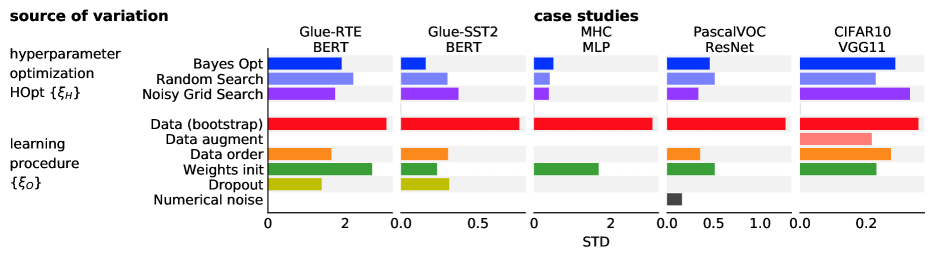
We selected i) the CIFAR10 (Krizhevsky et al., 2009) image classification with VGG11 (Simonyan & Zisserman, 2014), ii) PascalVOC (Everingham et al., ) image segmentation using an FCN Long et al. (2014) with a ResNet18 He et al. (2015a) backbone pretrained on imagenet Deng et al. (2009), iii-iv) Glue Wang et al. (2019) SST-2 Socher et al. (2013) and RTE Bentivogli et al. (2009) tasks with BERT Devlin et al. (2018) and v) peptide to major histocompatibility class I (MHC I) binding predictions with a shallow MLP. All details on default hyperparameters used and the computational environments –which used GPU years– can be found in Appendix D.
Variance in the learning procedure:
For the sources of variance from the learning procedure (), we identified: i) the data sampling, ii) data augmentation procedures, iii) model initialization, iv) dropout, and v) data visit order in stochastic gradient descent. We model the data-sampling variance as resulting from training the model on a finite dataset of size , sampled from an unknown true distribution. is thus a random variable, the standard source of variance considered in statistical learning. Since we have a single finite dataset in practice, we evaluate this variance by repeatedly generating a train set from bootstrap replicates of the data and measuring the out-of-bootstrap error Hothorn et al. (2005)222The more common alternative in machine learning is to use cross-validation, but the latter is less amenable to various sample sizes. Bootstrapping is discussed in more detail in Appendix B..
We first fixed hyperparameters to pre-selected reasonable choices333This choice is detailed in Appendix D.. Then, iteratively for each sources of variance, we randomized the seeds 200 times, while keeping all other sources fixed to initial values. Moreover, we measured the numerical noise with 200 training runs with all fixed seeds.
Figure 1 presents the individual variances due to sources from within the learning algorithms. Bootstrapping data stands out as the most important source of variance. In contrast, model initialization generally is less than 50% of the variance of bootstrap, on par with the visit order of stochastic gradient descent. Note that these different contributions to the variance are not independent, the total variance cannot be obtained by simply adding them up.
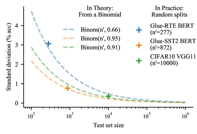
For classification, a simple binomial can be used to model the sampling noise in the measure of the prediction accuracy of a trained pipeline on the test set. Indeed, if the pipeline has a chance of giving the wrong answer on a sample, makes i.i.d. errors, and is measured on samples, the observed measure follows a binomial distribution of location parameter with degrees of freedom. If errors are correlated, not i.i.d., the degrees of freedom are smaller and the distribution is wider. Figure 2 compares standard deviations of the performance measure given by this simple binomial model to those observed when bootstrapping the data on the three classification case studies. The match between the model and the empirical results suggest that the variance due to data sampling is well explained by the limited statistical power in the test set to estimate the true performance.
Variance induced by hyperparameter optimization:
To study the sources of variation, we chose three of the most popular hyperparameter optimization methods: i) random search, ii) grid search, and iii) Bayesian optimization. While grid-search in itself has no random parameters, the specific choice of the parameter range is arbitrary and can be an uncontrolled source of variance (e.g., does the grid size step by powers of 2, 10, or increments of 0.25 or 0.5). We study this variance with a noisy grid search, perturbing slightly the parameter ranges (details in Appendix E).
For each of these tuning methods, we held all fixed to random values and executed 20 independent hyperparameter optimization procedures up to a budget of 200 trials. This way, all the observed variance across the hyperparameter optimization procedures is strictly due to . We were careful to design the search space so that it covers the optimal hyperparameter values (as stated in original studies) while being large enough to cover suboptimal values as well.
Results in figure 1 show that hyperparameter choice induces a sizable amount of variance, not negligible in comparison to the other factors. The full optimization curves of the 320 HPO procedures are presented in Appendix F. The three hyperparameter optimization methods induce on average as much variance as the commonly studied weights initialization. These results motivate further investigation the cost of ignoring the variance due to hyperparameter optimization.
The bigger picture: Variance matters
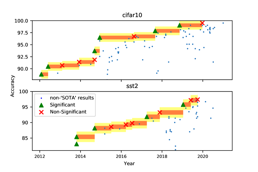
For a given case study, the total variance due to arbitrary choices and sampling noise revealed by our study can be put in perspective with the published improvements in the state-of-the-art. Figure 3 shows that this variance is on the order of magnitude of the individual increments. In other words, the variance is not small compared to the differences between pipelines. It must be accounted for when benchmarking pipelines.
3 Accounting for variance to reliably estimate performance
This section contains 1) an explanation of the counter intuitive result that accounting for more sources of variation reduces the standard error for an estimator of and 2) an empirical measure of the degradation of expected empirical risk estimation due to neglecting variance.
We will now consider different estimators of the average performance from Equation 2.1. Such estimators will use, in place of the expectation of Equation 2.1, an empirical average over (train+test) splits, which we will denote and the corresponding empirical variance. We will make an important distinction between an estimator which encompasses all sources of variation, the ideal estimator , and one which accounts only for a portion of these sources, the biased estimator .
But before delving into this, we will explain why many splits help estimating the expected empirical risk ().
3.1 Multiple data splits for smaller detectable improvements
The majority of machine-learning benchmarks are built with fixed training and test sets. The rationale behind this design, is that learning algorithms should be compared on the same grounds, thus on the same sets of examples for training and testing. While the rationale is valid, it disregards the fact that the fundamental ground of comparison is the true distribution from which the sets were sampled. This finite set is used to compute the expected empirical risk ( Eq 2.1), failing to compute the expected risk ( Eq 4) on the whole distribution. This empirical risk is therefore a noisy measure, it has some uncertainty because the risk on a particular test set gives limited information on what would be the risk on new data. This uncertainty due to data sampling is not small compared to typical improvements or other sources of variation, as revealed by our study in the previous section. In particular, figure 2 suggests that the size of the test set can be a limiting factor.
When comparing two learning algorithms and , we estimate their expected empirical risks with , a noisy measure. The uncertainty of this measure is represented by the standard error under the normal assumption444Our extensive numerical experiments show that a normal distribution is well suited for the fluctuations of the risk–figure G.3 of . This uncertainty is an important aspect of the comparison, for instance it appears in statistical tests used to draw a conclusion in the face of a noisy evidence. For instance, a z-test states that a difference of expected empirical risk between and of at least must be observed to control false detections at a rate of 95%. In other words, a difference smaller than this value could be due to noise alone, e.g. different sets of random splits may lead to different conclusions.
With , algorithms and must have a large difference of performance to support a reliable detection. In order to detect smaller differences, must be increased, i.e. must be computed over several data splits. The estimator is computationally expensive however, and most researchers must instead use a biased estimator that does not probe well all sources of variance.
3.2 Bias and variance of estimators depends on whether they account for all sources of variation
Probing all sources of variation, including hyperparameter optimization, is too computationally expensive for most researchers. However, ignoring the role of hyperparameter optimization induces a bias in the estimation of the expected empirical risk. We discuss in this section the expensive, unbiased, ideal estimator of and the cheap biased estimator of . We explain as well why accounting for many sources of variation improves the biased estimator by reducing its bias.
3.2.1 Ideal estimator: sampling multiple HOpt
The ideal estimator takes into account all sources of variation. For each performance measure , all and are randomized, each requiring an independent hyperparameter optimization procedure. The detailed procedure is presented in Algorithm 1. For an estimation over splits with hyperparameter optimization for a budget of trials, it requires fitting the learning algorithm a total of times. The estimator is unbiased, with .
For a variance of the performance measures , we can derive the variance of the ideal estimator by taking the sum of the variances in . We see that with . Thus is a well-behaved unbiased estimator of , as its mean squared error vanishes with infinitely large:
| (6) |
Note that does not appear in these equations. Yet it controls ’s runtime cost ( trials to determine ), and thus the variance is a function of .
Ideal Estimator
Biased Estimator
3.2.2 Biased estimator: fixing HOpt
A computationally cheaper but biased estimator consists in re-using the hyperparameters obtained from a single hyperparameter optimization to generate subsequent performance measures where only (or a subset of ) is randomized. This procedure is presented in Algorithm 2. It requires only fittings, substantially less than the ideal estimator. The estimator is biased with , . A bias will occur when a set of hyperparameters are optimal for a particular instance of but not over most others.
When we fix sources of variation to arbitrary values (e.g. random seed), we are conditioning the distribution of on some arbitrary . Intuitively, holding fix some sources of variations should reduce the variance of the whole process. What our intuition fails to grasp however, is that this conditioning to arbitrary induces a correlation between the trainings which in turns increases the variance of the estimator. Indeed, a sum of correlated variables increases with the strength of the correlations.
Let be the variance of the conditioned performance measures and the average correlation among all pairs of . The variance of the biased estimator is then given by the following equation.
| (7) |
We can see that with a large enough correlation , the variance could be dominated by the second term. In such case, increasing the number of data splits would not reduce the variance of . Unlike with , the mean square error for will not decreases with :
| (8) |
This result has two implications, one beneficial to improving benchmarks, the other not. Bad news first: the limited effectiveness of increasing to improve the quality of the estimator is a consequence of ignoring the variance induced by hyperparameter optimization. We cannot avoid this loss of quality if we do not have the budget for repeated independent hyperoptimization. The good news is that current practices generally account for only one or two sources of variation; there is thus room for improvement. This has the potential of decreasing the average correlation and moving closer to . We will see empirically in next section how accounting for more sources of variation moves us closer to in most of our case studies.
3.3 The cost of ignoring variance
To compare the estimators and presented above, we measured empirically the statistics of the estimators on budgets of points on our five case studies. The ideal estimator is asymptotically unbiased and therefore only one repetition is enough to estimate for each task. For the biased estimator we run 20 repetitions to estimate . We sample 20 arbitrary (random seeds) and compute the standard deviation of for .
We compared the biased estimator FixedHOptEst() while varying different subset of sources of variations to see if randomizing more of them would help increasing the quality of the estimator. We note FixedHOptEst(,Init) the biased estimator randomizing only the weights initialization, FixedHOptEst(,Data) the biased estimator randomizing only data splits, and FixedHOptEst(,All) the biased estimator randomizing all sources of variation except for hyperparameter optimization.
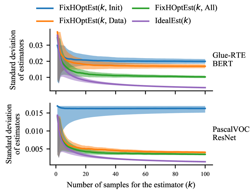
We present results from a subset of the tasks in Figure 5 (all tasks are presented in Figure H.4). Randomizing weights initialization only (FixedHOptEst(,init)) provides only a small improvement with . In the task where it best performs (Glue-RTE), it converges to the equivalent of . This is an important result since it corresponds to the predominant approach used in the literature today. Bootstrapping with FixedHOptEst(,Data) improves the standard error for all tasks, converging to equivalent of to . Still, the biased estimator including all sources of variations excluding hyperparameter optimization FixedHOptEst(,All) is by far the best estimator after the ideal estimator, converging to equivalent of to .
This shows that accounting for all sources of variation reduces the likelihood of error in a computationally achievable manner. IdealEst() takes 1 070 hours to compute, compared to only 21 hours for each FixedHOptEst(). Our study paid the high computational cost of multiple rounds of FixedHOptEst(,All), and the cost of IdealEst() for a total of 6.4 GPU years to show that FixedHOptEst(,All) is better than the status-quo and a satisfying option for statistical model comparisons without these prohibitive costs.
4 Accounting for variance to draw reliable conclusions
4.1 Criteria used to conclude from benchmarks
Given an estimate of the performance of two learning pipelines and their variance, are these two pipelines different in a meaningful way? We first formalize common practices to draw such conclusions, then characterize their error rates.
Comparing the average difference
A typical criterion to conclude that one algorithm is superior to another is that one reaches a performance superior to another by some (often implicit) threshold . The choice of the threshold can be arbitrary, but a reasonable one is to consider previous accepted improvements, e.g. improvements in Figure 3.
This difference in performance is sometimes computed across a single run of the two pipelines, but a better practice used in the deep-learning community is to average multiple seeds Bouthillier & Varoquaux (2020). Typically hyperparameter optimization is performed for each learning algorithm and then several weights initializations or other sources of fluctuation are sampled, giving estimates of the risk – note that these are biased as detailed in subsubsection 3.2.2. If an algorithm performs better than an algorithm by at least on average, it is considered as a better algorithm than for the task at hand. This approach does not account for false detections and thus can not easily distinguish between true impact and random chance.
Let , where is the empirical risk of algorithm on the -th split, be the mean performance of algorithm , and similarly for . The decision whether outperforms is then determined by .
The variance is not accounted for in the average comparison. We will now present a statistical test accounting for it. Both comparison methods will next be evaluated empirically using simulations based on our case studies.
Probability of outperforming
The choice of threshold is problem-specific and does not relate well to a statistical improvement. Rather, we propose to formulate the comparison in terms of probability of improvement. Instead of comparing the average performances, we compare their distributions altogether. Let be the probability of measuring a better performance for than across fluctuations such as data splits and weights initialization. To consider an algorithm significantly better than , we ask that outperforms often enough: . Often enough, as set by , needs to be defined by community standards, which we will revisit below. This probability can simply be computed as the proportion of successes, , where are pairs of empirical risks measured on different data splits for algorithms and .
| (9) |
where is the indicator function. We will build upon the non-parametric Mann-Whitney test to produce decisions about whether Perme & Manevski (2019) .
The problem is well formulated in the Neyman-Pearson view of statistical testing Neyman & Pearson (1928); Perezgonzalez (2015), which requires the explicit definition of both a null hypothesis to control for statistically significant results, and an alternative hypothesis to declare results statistically meaningful. A statistically significant result is one that is not explained by noise, the null-hypothesis . With large enough sample size, any arbitrarily small difference can be made statistically significant. A statistically meaningful result is one large enough to satisfy the alternative hypothesis . Recall that is a threshold that needs to be defined by community standards. We will discuss reasonable values for in next section based on our simulations.
We recommend to conclude that algorithm is better than on a given task if the result is both statistically significant and meaningful. The reliability of the estimation of can be quantified using confidence intervals, computed with the non-parametric percentile bootstrap Efron (1982). The lower bound of the confidence interval controls if the result is significant , and the upper bound of the confidence interval controls if the result is meaningful .
4.2 Characterizing errors of these conclusion criteria
We now run an empirical study of the two conclusion criteria presented above, the popular comparison of average differences and our recommended probability of outperforming. We will re-use mean and variance estimates from subsection 3.3 with the ideal and biased estimators to simulate performances of trained algorithms so that we can measure the reliability of these conclusion criteria when using ideal or biased estimators.
Simulation of algorithm performances
We simulate realizations of the ideal estimator and the biased estimator with a budget of data splits. For the ideal estimator, we model with a normal distribution , where is the variance measured with the ideal estimator in our case studies, and is the empirical risk . Our experiments consist in varying the difference in for the two algorithms, to span from identical to widely different performance ().
For the biased estimator, we rely on a two stage sampling process for the simulation. First, we sample the bias of based on the variance measured in our case studies, . Given , a sample of , we sample empirical risks following , where is the variance of the empirical risk averaged across 20 realizations of that we measured in our case studies.
In simulation we vary the mean performance of with respect to the mean performance of so that varies from 0.4 to 1 to test three regions:
- is true
-
: Not significant, not meaningful
- & are false ()
-
: Significant, not meaningful
- is true
-
: Significant and meaningful
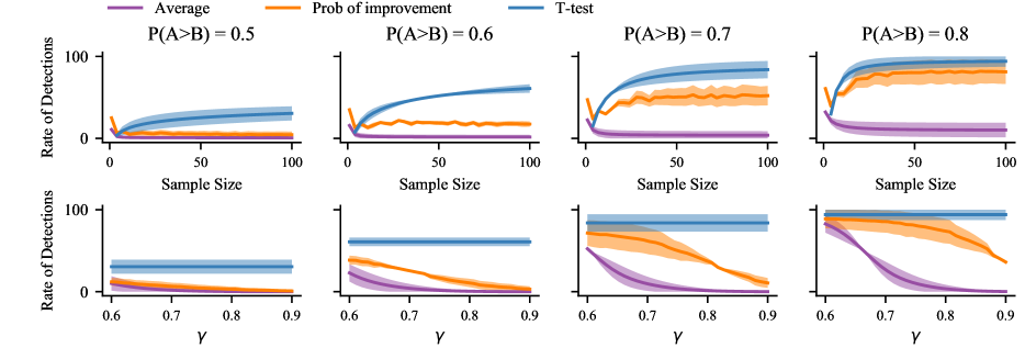
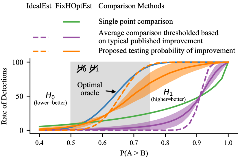
For decisions based on comparing averages, we set where is the standard deviation measured in our case studies with the ideal estimator. The value 1.9952 is set by linear regression so that matches the average improvements obtained from paperswithcode.com. This provides a threshold representative of the published improvements. For the probability of outperforming, we use a threshold of which we have observed to be robust across all case studies (See Appendix I).
Observations
Figure 6 reports results for different decision criteria, using the ideal estimator and the biased estimator, as the difference in performance of the algorithms and increases (x-axis). The x-axis is broken into three regions: 1) Leftmost is when is true (not-significant). 2) The grey middle when the result is significant, but not meaningful in our framework (). 3) The rightmost is when is true (significant and meaningful). The single point comparison leads to the worst decision by far. It suffers from both high false positives () and high false negatives (). The average with , on the other hand, is very conservative with low false positives () but very high false negatives (). Using the probability of outperforming leads to better balanced decisions, with a reasonable rate of false positives () on the left and a reasonable rate of false negatives on the right ().
The main problem with the average comparison is the threshold. A t-test only differs from an average in that the threshold is computed based on the variance of the model performances and the sample size. It is this adjustment of the threshold based on the variance that allows better control on false negatives.
Finally, we observe that the test of probability of outperforming () controls well the error rates even when used with a biased estimator. Its performance is nevertheless impacted by the biased estimator compared to the ideal estimator. Although we cannot guarantee a nominal control, we confirm that it is a major improvement compared to the commonly used comparison method at no additional cost.
5 Our recommendations: good benchmarks with a budget
We now distill from the theoretical and empirical results of the previous sections a set of practical recommendations to benchmark machine-learning pipelines. Our recommendations are pragmatic in the sense that they are simple to implement and cater for limited computational budgets.
Randomize as many sources of variations as possible
Fitting and evaluating a modern machine-learning pipeline comes with many arbitrary aspects, such as the choice of initializations or the data order. Benchmarking a pipeline given a specific instance of these choices will not give an evaluation that generalize to new data, even drawn from the same distribution. On the opposite, a benchmark that varies these arbitrary choices will not only evaluate the associated variance (section 2), but also reduce the error on the expected performance as they enable measures of performance on the test set that are less correlated (3). This counter-intuitive phenomenon is related to the variance reduction of bagging Breiman (1996a); Bühlmann et al. (2002), and helps characterizing better the expected behavior of a machine-learning pipeline, as opposed to a specific fit.
Use multiple data splits
The subset of the data used as test set to validate an algorithm is arbitrary. As it is of a limited size, it comes with a limited estimation quality with regards to the performance of the algorithm on wider samples of the same data distribution (figure 2). Improvements smaller than this variance observed on a given test set will not generalize. Importantly, this variance is not negligible compared to typical published improvements or other sources of variance (figures 1 and 3). For pipeline comparisons with more statistical power, it is useful to draw multiple tests, for instance generating random splits with a out-of-bootstrap scheme (detailed in appendix B).
Account for variance to detect meaningful improvements
Concluding on the significance –statistical or practical– of an improvement based on the difference between average performance requires the choice of a threshold that can be difficult to set. A natural scale for the threshold is the variance of the benchmark, but this variance is often unknown before running the experiments. Using the probability of outperforming with a threshold of gives empirically a criterion that separates well benchmarking fluctuations from published improvements over the 5 case studies that we considered. We recommend to always highlight not only the best-performing procedure, but also all those within the significance bounds. We provide an example in Appendix C to illustrate the application of our recommended statistical test.
6 Additional considerations
There are many aspects of benchmarks which our study has not addressed. For completeness, we discuss them here.
Comparing models instead of procedures
Our framework provides value when the user can control the model training process and source of variation. In cases where models are given but not under our control (e.g., purchased via API or a competition), the only source of variation left is the data used to test the model. Our framework and analysis does not apply to such scenarios.
Benchmarks and competitions with many contestants
We focused on comparing two learning algorithms. Benchmarks – and competitions in particular – commonly involve large number of learning algorithms that are being compared. Part of our results carry over unchanged in such settings, in particular those related to variance and performance estimation. With regards to reaching a well-controlled decision, a new challenge comes from multiple comparisons when there are many algorithms. A possible alley would be to adjust the decision threshold , raising it with a correction for multiple comparisons (e.g. Bonferroni) Dudoit et al. (2003). However, as the number gets larger, the correction becomes stringent. In competitions where the number of contestants can reach hundreds, the choice of a winner comes necessarily with some arbitrariness: a different choice of test sets might have led to a slightly modified ranking.
Comparisons across multiple dataset
Comparison over multiple datasets is often used to accumulate evidence that one algorithm outperforms another one. The challenge is to account for different errors, in particular different levels of variance, on each dataset.
Demšar (2006) recommended Wilcoxon signed ranks test or Friedman tests to compare classifiers across multiple datasets. These recommendations are however hardly applicable on small sets of datasets – machine learning works typically include as few as 3 to 5 datasets Bouthillier & Varoquaux (2020). The number of datasets corresponds to the sample size of these tests, and such a small sample size leads to tests of very limited statistical power.
Dror et al. (2017) propose to accept methods that give improvements on all datasets, controlling for multiple comparisons. As opposed to Demšar (2006)’s recommendation, this approach performs well with a small number of datasets. On the other hand, a large number of datasets will increase significantly the severity of the family-wise error-rate correction, making Demšar’s recommendations more favorable.
Non-normal metrics
We focused on model performance, but model evaluation in practice can include other metrics such as the training time to reach a performance level or the memory foot-print Reddi et al. (2020). Performance metrics are generally averages over samples which typically makes them amenable to a reasonable normality assumption.
7 Conclusion
We showed that fluctuations in the performance measured by machine-learning benchmarks arise from many different sources. In deep learning, most evaluations focus on the effect of random weight initialization, which actually contribute a small part of the variance, on par with residual fluctuations of hyperparameter choices after their optimization but much smaller than the variance due to perturbing the split of the data in train and test sets. Our study clearly shows that these factors must be accounted to give reliable benchmarks. For this purpose, we study estimators of benchmark variance as well as decision criterion to conclude on an improvement. Our findings outline recommendations to improve reliability of machine learning benchmarks: 1) randomize as many sources of variations as possible in the performance estimation; 2) prefer multiple random splits to fixed test sets; 3) account for the resulting variance when concluding on the benefit of an algorithm over another.
References
- Anders Sogaard & Alonso (2014) Anders Sogaard, Anders Johannsen, B. P. D. H. and Alonso, H. M. What’s in a p-value in nlp? In Proceedings of the Eighteenth Conference on Computational Natural Language Learning, pp. 1–10. Association for Computational Linguistics, 2014.
- Bentivogli et al. (2009) Bentivogli, L., Dagan, I., Dang, H. T., Giampiccolo, D., and Magnini, B. The fifth PASCAL recognizing textual entailment challenge. 2009.
- Blalock et al. (2020) Blalock, D., Gonzalez Ortiz, J. J., Frankle, J., and Guttag, J. What is the State of Neural Network Pruning? In Proceedings of Machine Learning and Systems 2020, pp. 129–146. 2020.
- Bouckaert & Frank (2004) Bouckaert, R. R. and Frank, E. Evaluating the replicability of significance tests for comparing learning algorithms. In Pacific-Asia Conference on Knowledge Discovery and Data Mining, pp. 3–12. Springer, 2004.
- Bouthillier & Varoquaux (2020) Bouthillier, X. and Varoquaux, G. Survey of machine-learning experimental methods at NeurIPS2019 and ICLR2020. Research report, Inria Saclay Ile de France, January 2020. URL https://hal.archives-ouvertes.fr/hal-02447823.
- Bouthillier et al. (2019) Bouthillier, X., Laurent, C., and Vincent, P. Unreproducible research is reproducible. In Chaudhuri, K. and Salakhutdinov, R. (eds.), Proceedings of the 36th International Conference on Machine Learning, volume 97 of Proceedings of Machine Learning Research, pp. 725–734, Long Beach, California, USA, 09–15 Jun 2019. PMLR. URL http://proceedings.mlr.press/v97/bouthillier19a.html.
- Breiman (1996a) Breiman, L. Bagging predictors. Machine learning, 24(2):123–140, 1996a.
- Breiman (1996b) Breiman, L. Out-of-bag estimation. 1996b.
- Bühlmann et al. (2002) Bühlmann, P., Yu, B., et al. Analyzing bagging. The Annals of Statistics, 30(4):927–961, 2002.
- Canty et al. (2006) Canty, A. J., Davison, A. C., Hinkley, D. V., and Ventura, V. Bootstrap diagnostics and remedies. Canadian Journal of Statistics, 34(1):5–27, 2006.
- Dacrema et al. (2019) Dacrema, M. F., Cremonesi, P., and Jannach, D. Are we really making much progress? A Worrying Analysis of Recent Neural Recommendation Approaches. In Proceedings of the 13th ACM Conference on Recommender Systems - RecSys ’19, pp. 101–109, New York, New York, USA, 2019. ACM Press. ISBN 9781450362436. doi: 10.1145/3298689.3347058. URL http://dl.acm.org/citation.cfm?doid=3298689.3347058.
- Demšar (2006) Demšar, J. Statistical comparisons of classifiers over multiple data sets. Journal of Machine learning research, 7(Jan):1–30, 2006.
- Deng et al. (2009) Deng, J., Dong, W., Socher, R., Li, L.-J., Li, K., and Fei-Fei, L. ImageNet: A Large-Scale Hierarchical Image Database. In CVPR09, 2009.
- Devlin et al. (2018) Devlin, J., Chang, M.-W., Lee, K., and Toutanova, K. Bert: Pre-training of deep bidirectional transformers for language understanding, 2018.
- Dietterich (1998) Dietterich, T. G. Approximate statistical tests for comparing supervised classification learning algorithms. Neural computation, 10(7):1895–1923, 1998.
- Dror et al. (2017) Dror, R., Baumer, G., Bogomolov, M., and Reichart, R. Replicability analysis for natural language processing: Testing significance with multiple datasets. Transactions of the Association for Computational Linguistics, 5:471–486, 2017.
- Dudoit et al. (2003) Dudoit, S., Shaffer, J. P., and Boldrick, J. C. Multiple hypothesis testing in microarray experiments. Statistical Science, pp. 71–103, 2003.
- Efron (1979) Efron, B. Bootstrap methods: Another look at the jackknife. Ann. Statist., 7(1):1–26, 01 1979. doi: 10.1214/aos/1176344552. URL https://doi.org/10.1214/aos/1176344552.
- Efron (1982) Efron, B. The jackknife, the bootstrap, and other resampling plans, volume 38. Siam, 1982.
- Efron & Tibshirani (1994) Efron, B. and Tibshirani, R. J. An introduction to the bootstrap. CRC press, 1994.
- (21) Everingham, M., Van Gool, L., Williams, C. K. I., Winn, J., and Zisserman, A. The PASCAL Visual Object Classes Challenge 2012 (VOC2012) Results. http://www.pascal-network.org/challenges/VOC/voc2012/workshop/index.html.
- Glorot & Bengio (2010) Glorot, X. and Bengio, Y. Understanding the difficulty of training deep feedforward neural networks. In Teh, Y. W. and Titterington, M. (eds.), Proceedings of the Thirteenth International Conference on Artificial Intelligence and Statistics, volume 9 of Proceedings of Machine Learning Research, pp. 249–256, Chia Laguna Resort, Sardinia, Italy, 13–15 May 2010. PMLR. URL http://proceedings.mlr.press/v9/glorot10a.html.
- Gorman & Bedrick (2019) Gorman, K. and Bedrick, S. We need to talk about standard splits. In Proceedings of the 57th Annual Meeting of the Association for Computational Linguistics, pp. 2786–2791, Florence, Italy, July 2019. Association for Computational Linguistics. doi: 10.18653/v1/P19-1267. URL https://www.aclweb.org/anthology/P19-1267.
- He et al. (2015a) He, K., Zhang, X., Ren, S., and Sun, J. Deep residual learning for image recognition, 2015a.
- He et al. (2015b) He, K., Zhang, X., Ren, S., and Sun, J. Delving deep into rectifiers: Surpassing human-level performance on imagenet classification. In Proceedings of the IEEE international conference on computer vision, pp. 1026–1034, 2015b.
- He et al. (2016) He, K., Zhang, X., Ren, S., and Sun, J. Identity mappings in deep residual networks. In European conference on computer vision, pp. 630–645. Springer, 2016.
- Henderson et al. (2018) Henderson, P., Islam, R., Bachman, P., Pineau, J., Precup, D., and Meger, D. Deep reinforcement learning that matters. In Thirty-Second AAAI Conference on Artificial Intelligence, 2018.
- Henikoff & Henikoff (1992) Henikoff, S. and Henikoff, J. G. Amino acid substitution matrices from protein blocks. Proceedings of the National Academy of Sciences, 89(22):10915–10919, 1992.
- Hothorn et al. (2005) Hothorn, T., Leisch, F., Zeileis, A., and Hornik, K. The design and analysis of benchmark experiments. Journal of Computational and Graphical Statistics, 14(3):675–699, 2005.
- Hutter et al. (2014) Hutter, F., Hoos, H., and Leyton-Brown, K. An efficient approach for assessing hyperparameter importance. In Proceedings of International Conference on Machine Learning 2014 (ICML 2014), pp. 754–762, June 2014.
- Jurtz et al. (2017) Jurtz, V., Paul, S., Andreatta, M., Marcatili, P., Peters, B., and Nielsen, M. Netmhcpan-4.0: improved peptide–mhc class i interaction predictions integrating eluted ligand and peptide binding affinity data. The Journal of Immunology, 199(9):3360–3368, 2017.
- Kadlec et al. (2017) Kadlec, R., Bajgar, O., and Kleindienst, J. Knowledge base completion: Baselines strike back. In Proceedings of the 2nd Workshop on Representation Learning for NLP, pp. 69–74, 2017.
- Kingma & Welling (2014) Kingma, D. P. and Welling, M. Auto-encoding variational bayes. In Bengio, Y. and LeCun, Y. (eds.), 2nd International Conference on Learning Representations, ICLR 2014, Banff, AB, Canada, April 14-16, 2014, Conference Track Proceedings, 2014. URL http://arxiv.org/abs/1312.6114.
- Klein et al. (2017) Klein, A., Falkner, S., Mansur, N., and Hutter, F. Robo: A flexible and robust bayesian optimization framework in python. In NIPS 2017 Bayesian Optimization Workshop, December 2017.
- Krizhevsky et al. (2009) Krizhevsky, A., Hinton, G., et al. Learning multiple layers of features from tiny images. 2009.
- Liu et al. (2018) Liu, C., Zoph, B., Neumann, M., Shlens, J., Hua, W., Li, L.-J., Fei-Fei, L., Yuille, A., Huang, J., and Murphy, K. Progressive neural architecture search. In The European Conference on Computer Vision (ECCV), September 2018.
- Long et al. (2014) Long, J., Shelhamer, E., and Darrell, T. Fully convolutional networks for semantic segmentation, 2014.
- Lucic et al. (2018) Lucic, M., Kurach, K., Michalski, M., Gelly, S., and Bousquet, O. Are gans created equal? a large-scale study. In Bengio, S., Wallach, H., Larochelle, H., Grauman, K., Cesa-Bianchi, N., and Garnett, R. (eds.), Advances in Neural Information Processing Systems 31, pp. 700–709. Curran Associates, Inc., 2018.
- Maddison et al. (2017) Maddison, C. J., Mnih, A., and Teh, Y. W. The concrete distribution: A continuous relaxation of discrete random variables. In 5th International Conference on Learning Representations, ICLR 2017, Toulon, France, April 24-26, 2017, Conference Track Proceedings. OpenReview.net, 2017. URL https://openreview.net/forum?id=S1jE5L5gl.
- Mahajan et al. (2018) Mahajan, D., Girshick, R., Ramanathan, V., He, K., Paluri, M., Li, Y., Bharambe, A., and van der Maaten, L. Exploring the limits of weakly supervised pretraining. In Proceedings of the European Conference on Computer Vision (ECCV), pp. 181–196, 2018.
- Melis et al. (2018) Melis, G., Dyer, C., and Blunsom, P. On the state of the art of evaluation in neural language models. ICLR, 2018.
- Musgrave et al. (2020) Musgrave, K., Belongie, S., and Lim, S.-N. A Metric Learning Reality Check. arXiv, 2020. URL http://arxiv.org/abs/2003.08505.
- Nadeau & Bengio (2000) Nadeau, C. and Bengio, Y. Inference for the generalization error. In Solla, S. A., Leen, T. K., and Müller, K. (eds.), Advances in Neural Information Processing Systems 12, pp. 307–313. MIT Press, 2000.
- Neyman & Pearson (1928) Neyman, J. and Pearson, E. S. On the use and interpretation of certain test criteria for purposes of statistical inference: Part i. Biometrika, pp. 175–240, 1928.
- Nielsen et al. (2007) Nielsen, M., Lundegaard, C., Blicher, T., Lamberth, K., Harndahl, M., Justesen, S., Røder, G., Peters, B., Sette, A., Lund, O., et al. Netmhcpan, a method for quantitative predictions of peptide binding to any hla-a and-b locus protein of known sequence. PloS one, 2(8), 2007.
- Noether (1987) Noether, G. E. Sample size determination for some common nonparametric tests. Journal of the American Statistical Association, 82(398):645–647, 1987.
- O’Donnell et al. (2018) O’Donnell, T. J., Rubinsteyn, A., Bonsack, M., Riemer, A. B., Laserson, U., and Hammerbacher, J. Mhcflurry: open-source class i mhc binding affinity prediction. Cell systems, 7(1):129–132, 2018.
- Pearson et al. (2016) Pearson, H., Daouda, T., Granados, D. P., Durette, C., Bonneil, E., Courcelles, M., Rodenbrock, A., Laverdure, J.-P., Côté, C., Mader, S., et al. Mhc class i–associated peptides derive from selective regions of the human genome. The Journal of clinical investigation, 126(12):4690–4701, 2016.
- Perezgonzalez (2015) Perezgonzalez, J. D. Fisher, neyman-pearson or nhst? a tutorial for teaching data testing. Frontiers in Psychology, 6:223, 2015.
- Perme & Manevski (2019) Perme, M. P. and Manevski, D. Confidence intervals for the mann–whitney test. Statistical methods in medical research, 28(12):3755–3768, 2019.
- Raff (2019) Raff, E. A Step Toward Quantifying Independently Reproducible Machine Learning Research. In NeurIPS, 2019. URL http://arxiv.org/abs/1909.06674.
- Raff (2021) Raff, E. Research Reproducibility as a Survival Analysis. In The Thirty-Fifth AAAI Conference on Artificial Intelligence, 2021. URL http://arxiv.org/abs/2012.09932.
- Reddi et al. (2020) Reddi, V. J., Cheng, C., Kanter, D., Mattson, P., Schmuelling, G., Wu, C.-J., Anderson, B., Breughe, M., Charlebois, M., Chou, W., et al. Mlperf inference benchmark. In 2020 ACM/IEEE 47th Annual International Symposium on Computer Architecture (ISCA), pp. 446–459. IEEE, 2020.
- Reimers & Gurevych (2017) Reimers, N. and Gurevych, I. Reporting score distributions makes a difference: Performance study of LSTM-networks for sequence tagging. In Proceedings of the 2017 Conference on Empirical Methods in Natural Language Processing, pp. 338–348, Copenhagen, Denmark, September 2017. Association for Computational Linguistics. doi: 10.18653/v1/D17-1035. URL https://www.aclweb.org/anthology/D17-1035.
- Riezler & Maxwell (2005) Riezler, S. and Maxwell, J. T. On some pitfalls in automatic evaluation and significance testing for mt. In Proceedings of the ACL Workshop on Intrinsic and Extrinsic Evaluation Measures for Machine Translation and/or Summarization, pp. 57–64, 2005.
- Simonyan & Zisserman (2014) Simonyan, K. and Zisserman, A. Very deep convolutional networks for large-scale image recognition. arXiv preprint arXiv:1409.1556, 2014.
- Socher et al. (2013) Socher, R., Perelygin, A., Wu, J., Chuang, J., Manning, C. D., Ng, A., and Potts, C. Recursive deep models for semantic compositionality over a sentiment treebank. In Proceedings of EMNLP, pp. 1631–1642, 2013.
- Srivastava et al. (2014) Srivastava, N., Hinton, G., Krizhevsky, A., Sutskever, I., and Salakhutdinov, R. Dropout: A simple way to prevent neural networks from overfitting. Journal of Machine Learning Research, 15(56):1929–1958, 2014. URL http://jmlr.org/papers/v15/srivastava14a.html.
- Taylor Berg-Kirkpatrick & Klein (2012) Taylor Berg-Kirkpatrick, D. B. and Klein, D. An empirical investigation of statistical significance in nlp. In Proceedings of the 2012 Joint Conference on Empirical Methods in Natural Language Processing and Computational Natural Language Learning, pp. 995–1005. Association for Computational Linguistics, 2012.
- Torralba et al. (2008) Torralba, A., Fergus, R., and Freeman, W. T. 80 million tiny images: A large data set for nonparametric object and scene recognition. IEEE transactions on pattern analysis and machine intelligence, 30(11):1958–1970, 2008.
- Vaswani et al. (2017) Vaswani, A., Shazeer, N., Parmar, N., Uszkoreit, J., Jones, L., Gomez, A. N., Kaiser, L., and Polosukhin, I. Attention is all you need, 2017.
- Vita et al. (2019) Vita, R., Mahajan, S., Overton, J. A., Dhanda, S. K., Martini, S., Cantrell, J. R., Wheeler, D. K., Sette, A., and Peters, B. The immune epitope database (iedb): 2018 update. Nucleic acids research, 47(D1):D339–D343, 2019.
- Wang et al. (2019) Wang, A., Singh, A., Michael, J., Hill, F., Levy, O., and Bowman, S. R. GLUE: A multi-task benchmark and analysis platform for natural language understanding. 2019. In the Proceedings of ICLR.
- Wolf et al. (2019) Wolf, T., Debut, L., Sanh, V., Chaumond, J., Delangue, C., Moi, A., Cistac, P., Rault, T., Louf, R., Funtowicz, M., and Brew, J. Huggingface’s transformers: State-of-the-art natural language processing. ArXiv, abs/1910.03771, 2019.
- Xie et al. (2019) Xie, Q., Hovy, E., Luong, M.-T., and Le, Q. V. Self-training with noisy student improves imagenet classification. arXiv preprint arXiv:1911.04252, 2019.
Appendix A Notes on reproducibility
Ensuring full reproducibility is often a tedious work. We provide here notes and remarks on the issues we encountered while working towards fully reproducible experiments.
The testing procedure
To ensure proper study of the sources of variation it was necessary to control them close to perfection. For all tasks, we ran a pipeline of tests to ensure perfect reproducibility at execution and also at resumption. During the tests, each source of variation was varied with 5 different seeds, each executed 5 times. This ensured that the pipeline was reproducible for different seeds. Additionally, for each source of variation and for each seed, another training was executed but automatically interrupted after each epoch. The worker would then start the training of the next seed and iterate through the trainings for all seeds before resuming the first one. All these tests uncovered many bugs and typical reproducibility issues in machine learning. We report here some notes.
Computer architecture & drivers
Although we did not measure the variance induced by different GPU architectures, we did observe that different GPU models would lead to different results. The CPU model had less impact on the Deep Learning tasks but the MLP-MHC task was sensitive to it. We therefore limited all tasks to specific computer architectures. We also observed issues when CUDA drivers were updated during preliminary experiments. We ensured all experiments were run using CUDA 10.2.
Software & seeds
PyTorch versions lead to different results as well. We ran every Deep Learning experiments with PyTorch 1.2.0.
We implemented our data pipeline so that we could seed the iterators, the data augmentation objects and the splitting of the datasets. We had less control at the level of the models however. For PyTorch 1.2.0, the random number generator (RNG) must be seeded globally which makes it difficult to seed different parts separately. We seeded PyTorch’s global RNG for weight initialization at the beginning of the training process and then seeded PyTorch’s RNG for the dropout. Afterwards we checkpoint the RNG state so that we can restore the RNG states at resumption. We found that models with convolutionnal layers would not yield reproducible results unless we enabled cudnn.deterministic and disabled cudnn.benchmark.
We used the library RoBO Klein et al. (2017) for our Bayesian Optimizer. There was no support for seeding, we therefore resorted to seeding the global seed of python and numpy random number generators. We needed again to keep track of the RNG states and checkpoint them so that we can resume the Bayesian Optimizer without harming the reproducibility.
For one of our case study, image segmentation, we have been unable to make the learning pipeline perfectly reproducible. This is problematic because it prevents us from studying each source of variation in isolation. We thus trained our model with every seeds fixed across all 200 trainings and measured the variance we could not control. This is represented as the numerical noise in Figures 1 and G.3.
Appendix B Our bootstrap procedure
Cross-validation with different impacts the number of samples, it is not the case with not bootstrap. That means flexible sample sizes for statistical tests is hardly possible with cross-validation within affecting the training dataset sizes. Hothorn et al. (2005) focuses on the dataset sampling as the most important source of variation and marginalize out all other sources by taking the average performance over multiple runs for a given dataset. This increases even more the computational cost of the statistical tests.
We probe the effect of data sampling with bootstrap, specifically by bootstrapping to generate training sets and measuring the out-of-bootstrap error, as introduced by Breiman (1996b) in the context of bagging and generalized by Hothorn et al. (2005). For completeness, we formalize this use of the bootstrap to create training and test sets and how it can estimate the variance of performance measure due to data sampling on a finite dataset.
We assume we are seeking to generate sets of i.i.d. samples from true distribution . Ideally we would have access to and could sample our finite datasets independently from it.
| (10) |
Instead we have one dataset of finite size and need to sample independent datasets from it. A popular method in machine learning to estimate performance on a small dataset is cross-validation Bouckaert & Frank (2004); Dietterich (1998). This method however underestimates variance because of correlations induced by the process. We instead favor bootstrapping Efron (1979) as used by Hothorn et al. (2005) to simulate independent data sampling from the true distribution.
| (11) |
Where represents sampling the -th training set with replacement from the set . We then turn to out-of-bootstrapping to generate the held-out set. We use all remaining samples in to sample .
| (12) |
This procedure is represented as in the empirical average risk , end of Section 2.1.
Appendix C Statistical testing
We are interested in asserting whether a learning algorithm better performs than another learning algorithm . Measuring the performance of these learning algorithms is not a deterministic process however and we may be deceived if noise is not accounted for. Because of the noise, we cannot know for sure whether a conclusion we draw is true, but using a statistical test, we can at least ensure a bounded rate of false positives (drawing while truth is ) and false negatives (drawing while truth is ). The capacity of a statistical test to identify true differences, that is, of correctly inferring when this is true, is called the statistical power of a test. The procedure we describe here seeks to avoid deception from false positives while providing a strong statistical power.
We will describe the entire procedure, from the generation of the performance measures (Sections C.1 & C.2), the estimation of sample size (Section C.3), computation of (Section C.4), computation of the confidence interval (Section C.5) to the inference based on the statistical test (Section C.6)
C.1 Randomizing sources of variance
As shown in Section 3, randomizing as many sources of variance as possible in the learning pipelines help reduce the correlation and thus improve the reliability of the performance estimation. The simplest way to randomize as many as possible is to simply avoid seeding the random number generators. We list here sources of variations we faced in our case studies, but there exists many other sources of variations in diverse learning algorithms and tasks.
- Data splits
-
The data being used should ideally always be different samples from the true distribution of interest. In practice we only have access to a finite dataset and therefore the best we can do is random splits with cross-validation or out-of-bootstrap as described in Appendix B.
- Data order
-
The ordering of the data can have a surprisingly important impact as can be observed in Figure 1.
- Data augmentation
-
Stochastic data augmentation should not be seeded, so that it follows a different sequence at each run.
- Model initialization
-
Model initialization, e.g. weights initialization in neural networks, should be randomized across all trainings.
- Model stochasticity
- Hyperparameter optimization
-
The optimization of the hyperparameters generally include stochasticity which should ideally be randomized. Running multiple hyperparameter optimizations may often be practically unaffordable. Tests may still be carried out while fixing the hyperparameters after a single hyperparameter optimization, but keep in mind the incurred degradation of the reliability of the conclusion as shown in Section 4.
C.2 Pairing
Pairing is optional but is highly recommended to increase statistical power. Avoiding seeding is the simplest solution for the randomization, but it is not the best solution. If possible, meticulously seeding all sources of variation with different random seeds at each run makes it possible to pair trainings of the algorithms so that we can conduct paired comparisons.
Pairing is a simple but powerful way of increasing the power of statistical tests, that is, enabling the reliable detection of difference with smaller sample sizes. Let and be the standard deviation of the performance metric of learning algorithms and respectively. If measures of and are not paired, the standard deviation of is then . If we pair them, then we marginalize out sources of variance which results in a smaller variance . This reduction of variance makes it possible to reliably detect smaller differences without increasing the sample size.
To pair the learning algorithms, sources of variation should be randomized similarly for all of them. For instance, the random split of the dataset obtained from out-of-bootstrap should be used for both and when making a comparison. Suppose we plan to execute 10 runs of and , then we should generate 10 different splits and train and on each. The performances would then be compared only on the corresponding splits . The same would apply to all other sources of variations. In practical terms, pairing and requires sampling seeds for each pairs, re-using the same seed for and in each pairs.
For some sources of variation it may not make sense to pair. This is the case for instance with weights initialization if and involve different neural network architectures. We can still pair. This would not help much, but would not hurt as well. In doubt, it is better to pair.
C.3 Sample size
As explained in Section 3, the more runs we have from and , the more reliable the estimate of is. Lets note this number of runs as the sample size , not to be confused with dataset size . There exist a way of computing the minimal sample size required to ensure a minimal rate of false negatives based on power analysis.
We must first set the threshold for our test. Based on our experiments in Section 4, we recommend a value of 0.75. We then set the desired rates of false positives and false negatives with and respectively. Usual value for is 0.05 while ranges from 0.05 to 0.2. We recommend for a strong statistical power.
The estimation of is equivalent to a Mann–Whitney test Perme & Manevski (2019), thus we can use Noether’s sample size determination method for this type of test Noether (1987).
Where is the inverse cumulative function of the normal distribution.
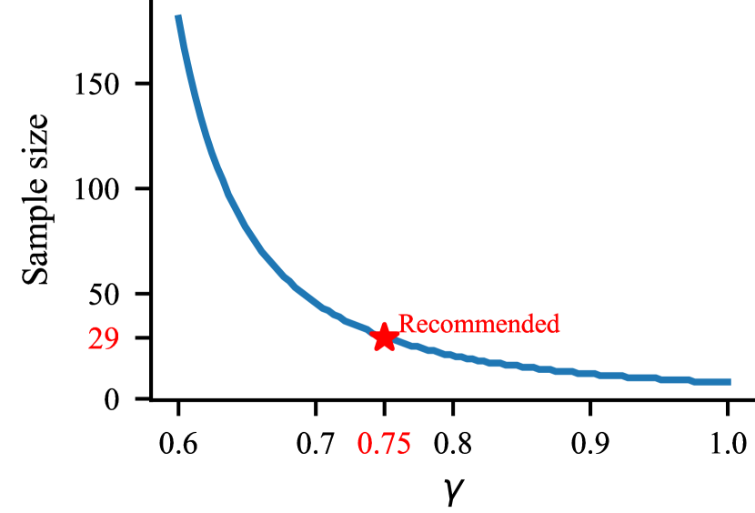
Figure C.1 shows how the minimal sample size evolves with . Detecting below is unpractical, requiring more that 700 trainings below 0.55 for instance. For a threshold that is representative of the published improvements as presented in Figure 3, , the minimal sample size required to ensure a rate of 5% false negatives (as defined by ) is reasonably small; 29 trainings.
C.4 Compute
C.5 Confidence interval of with percentile bootstrap
For the estimation of with values below 0.95, we recommend the use of the the percentile bootstrap555 Percentile bootstrap is not always reliable depending on the underlying distribution and resampling methods but should generally be good for distributions of of learning algorithms below 0.95. See Canty et al. (2006) for a discussion on the topic. Efron & Tibshirani (1994).
Suppose we have pairs . To compute the percentile bootstrap, we first generate groups of pairs. To do so, we sample with replacement pairs, and do so independently times. For each of the groups, we compute . We sort the estimations of and pick the -percentile and - percentile as the lower and upper bounds. The confidence interval is defined as these lower and upper bounds computed with percentile bootstrap.
C.6 Statistical test with
Let and be the lower and upper bounds of the confidence interval. We draw a conclusion based on the three following scenarios.
-
: Not statistically significant. No conclusion should be drawn as the result could be explained by noise alone.
-
: Not statistically meaningful. Perhaps but it is irrelevant since is too small to be meaningful.
-
: Statistically significant and meaningful. We can conclude that learning algorithm is better performing than in the conditions defined by the experiments.
Appendix D Case studies
D.1 CIFAR10 Image classification with VGG11
Task
CIFAR10 Krizhevsky et al. (2009) is a dataset of 60,000 32x32 color images selected from 80 million tiny images dataset Torralba et al. (2008), divided in 10 balanced classes. The original split contains 50,000 images for training and 10,000 images for testing. We applied random cropping and random horizontal flipping data augmentations.
Bootstrapping
The aggregation of all original training and testing samples are used for the bootstrap. To preserve the balance of the classes, we applied stratified bootstrap. For each class separately, we sampled with replacement 4,000 training samples, 1,000 for validation and 1,000 for testing. As for all tasks, we use out-of-bootstrap to ensure samples cannot be contained in more than one set.
Model
Search space for hyperparameters
We focused on learning rate, weight decay, momentum and learning rate schedule. Batch-size was omitted to simplify the multi-model training on GPUs, so that memory usage was consistent and predictable across all hyperparameter settings. To ease the definition of the search space for the learning rate schedule, we used exponential decay instead of multi-step decay despite the wide use of the latter with similar tasks and models Simonyan & Zisserman (2014); Xie et al. (2019); Mahajan et al. (2018); Liu et al. (2018); He et al. (2016; 2015b). The former only require tuning of while the later requires additionally selecting number of steps. Search space for all experiments and default values used for the variance experiments are presented in Table 2.
| Hardware/Software | Type/Version |
|---|---|
| CPU | Intel(R) Xeon(R) Gold |
| 6148 CPU @ 2.40GHz | |
| GPU model | Tesla V100-SXM2-16GB |
| GPU driver | 440.33.01 |
| OS | CentOS 7.7.1908 Core |
| Python | 3.6.3 |
| PyTorch | 1.2.0 |
| CUDA | 10.2 |
| Hyperparameters | Default | Space |
| learning rate | 0.03 | log(, ) |
| weight decay | 0.002 | log(, ) |
| momentum | 0.9 | lin(, ) |
| of lr schedule | 0.97 | lin(, ) |
| batch-size | 128 | - |
| Hyperparameters | Default | Space |
|---|---|---|
| learning rate | log(, ) | |
| weight decay | log(, ) | |
| std for weights init. | log(, ) | |
| 0.9 | - | |
| 0.999 | - | |
| dropout rate | - | |
| batch size | 32 | - |
D.2 Glue-SST2 sentiment prediction with BERT
Task
SST2 (Stanford Sentiment Treebank) Socher et al. (2013) is a binary classification task included in GLUE Wang et al. (2019). In this task, the input is a sentence from a collection of movie reviews, and the target is the associated sentiment (either positive or negative). The publicly available data contains around 68k entries.
Bootstrapping
We maintained the same size ratio between train/validation (i.e., 0.013) when performing the bootstrapping analysis. We performed standard out-of-bootstrap without conserving class balance since the original dataset is not balanced and ratios between classes vary from training and validation set in the original splits. The variable ratios of classes across bootstrap samples generate additional variance in our results, but is representative of the effect of generating a dataset that is not perfectly balanced.
Model
We used the BERT Devlin et al. (2018) implementation provided by the Hugging Face Wolf et al. (2019) repository. BERT is a Transformer Vaswani et al. (2017) encoder pre-trained on the self-supervised Masked Language Model task Devlin et al. (2018). We chose BERT given its importance and influence in the NLP literature. It is worthy to note that the pre-training phase of BERT is also affected by sources of variations. Nevertheless, we didn’t investigate this phase given the amount of time (and resources) required to perform it. Instead, we always start from the (same) pre-trained model image provided by the Hugging Face Wolf et al. (2019) repository. Indeed, the weight initialization was only applied to the final classifier. The initialization method used is standard Gaussian with mean and standard deviation that depends on the related hyperparameter.
Search space of hyperparameters
We ran a small-scale hyperparameter space exploration in order to select the hyperparameter search space to use in our experiments. As such, we decided to include the learning rate, weight decay and the standard deviation for the model parameter initialization (see Table 3). We fixed the dropout probability to the value of 0.1 as in the original BERT architecture. For the same reason, we fixed and . Default values used for the variance experiments are also reported in Table 3. The model has been fine-tuned on SST2 for 3 epochs, with a batch size of 32. Training has been performed with mixed precision. Note that for weight decay we used the default value from the Hugging Face repository (i.e., ) even if this is outside of the hyperparameter search space. We confirmed that this makes no difference by looking at the results of the small-scale hyperparameter space exploration.
D.3 Glue-RTE entailment prediction with BERT
Task
RTE (Recognizing Textual Entailment) Bentivogli et al. (2009) is a also a binary classification task included in GLUE Wang et al. (2019). The task is a collection of text fragment pairs, and the target is to predict if the first text fragment entails the second one. RTE dataset only contains around 2.5k entries.
Bootstrapping
In our bootstrapping analysis we maintained the train/validation ratio of 0.1. As for Glue-SST2, we used standard out-of-bootstrap and did not preserve original class ratios.
Model & search space of hyperparameters
We used the BERT Devlin et al. (2018) model for RTE as well, trained in the same way specified in the SST-2 section. In particular, we used the same hyperparameters (see Table 3), same batch size, and we trained in the same mixed-precision environment. The model has been fine-tuned on RTE for 3 epochs.
D.4 PascalVOC image segmentation with ResNet Backbone
Task
The PascalVOC segmentation task Everingham et al. entails generating pixel-level segmentations to classify each pixel in an image as one of 20 classes or background. This publicly available dataset contains 2913 images and associated ground truth segmentation labels. The original splits contains 2184 images for training and 729 for validation. Images were normalized and zero-padded to a final size of 512x512.
Bootstrapping
We used a train/validation ratio of 0.25 for our bootstrap analysis, generating training sets of 2184 images, validation and test sets of 729 images each. Since multiple classes can appear in a single image, the original dataset was not balanced, we thus used standard out-of-bootstrap for our experiments.
Model
We used an FCN-16s Long et al. (2014) with a ResNet18 backbone He et al. (2015a) pretrained on ImageNet Deng et al. (2009). After exploring several possible backbones, ResNet18 was selected since it could be trained relatively quickly. We use weighted cross entropy, with only predictions within the original image boundary contributing to the loss. The model is optimized using SGD with momentum.
Metric
The metric used is the mean Intersection over Union (mIoU) of the twenty classes and the background class. The complement of the mIoU, the mean Jaccard Distance, is the metric minimized in all HPO experiments.
Search space of hyperparameters
Certain hyperparmeters, such as the number of kernals, or the total number of layers, are part of the definition of the ResNet18 architecture. As a result, we explored key optimization hyperparameters including: learning rate, momentum, and weight decay. The hyperparameter ranges selected, as well as the default hyperparameters used in the variance experiments, can be found in table 5 and in table LABEL:table:hps-pascal-voc-default-appendix, respectively. A batch size of 16 was used for all experiments.
| Hardware/Software | Type/Version |
|---|---|
| CPU | Intel(R) Xeon(R) Silver |
| 4216 CPU @ 2.1GHz | |
| GPU model | Tesla V100 Volta 32G |
| GPU driver | 440.33.01 |
| OS | CentOS 7.7.1908 Core |
| Python | 3.6.3 |
| PyTorch | 1.2.0 |
| CUDA | 10.2 |
| Hyperparameters | Default | Space |
|---|---|---|
| learning rate | 0.002 | log(, ) |
| momentum | 0.9 | lin(, ) |
| weight decay | 0.000001 | log(, ) |
| batch-size | 16 | - |
D.5 Major histocompatibility class I-associated peptide binding prediction with shallow MLP
| Hyperparameters | Default | Space |
|---|---|---|
| hidden layer size | lin(, ) | |
| L2-weight decay | log(, ) |
| # HPs | Hyperparameters | Default Value |
|---|---|---|
| 1 | hidden layer size | 150 |
| 2 | L2-weight decay | 0.001 |
| Model name | Dataset | AUC | PCC |
| NetMHCpan4 | HPV | 0.53 | 0.39 |
| MHCflurry | HPV | 0.58 | 0.41 |
| MLP-MHC | HPV | 0.63 | 0.31 |
| NetMHCpan4 | NetMHC-CVsplits | 0.854 | 0.620 |
| MHCflurry | NetMHC-CVsplits | 0.964* | 0.671* |
| MLP-MHC | NetMHC-CVsplits | 0.861 | 0.660 |
| Model name | Inputs | Model design | Dataset | Sequence encoding |
|---|---|---|---|---|
| NetMHCpan4 | allele+peptide | shallow MLP | custom CV splitVita et al. (2019) | BLOSUM62 |
| MHCflurry | peptide | ensemble of shallow MLPs | O’Donnell et al. (2018) | BLOSUM62 |
| MLP-MHC | allele+peptide | shallow MLP | same as O’Donnell et al. (2018) | Sparse |
| Hardware/Software | Type/Version |
|---|---|
| CPU | Intel(R) Xeon(R) CPU E5-2640 v4 |
| 320 CPU @ 2.40GHz | |
| OS | CentOS 7.7.1908 Core |
| Python | 3.6.8 |
| sklearn | 0.22.2.post1 |
| BLAS | 3.4.2 |
Task
The MLP-MHC is a regression task with the goal of predicting the relative binding affinity for a given peptide and major histocompatibility complex class I (MHC) allele pair. The major histocompatibility complex (MHC) class I proteins are present on the surface of most nucleated cells in jawed vertebrates Pearson et al. (2016). These proteins bind short peptides that arise from the degradation of intra-cellular proteins Pearson et al. (2016). The complex of peptide-MHC molecule is used by immune cells to recognize healthy cells and eliminate cancerous or infected cells, a mechanism studied in the development of immunotherapy and vaccines O’Donnell et al. (2018). The peptide binding prediction task is therefore at the base of the search for good vaccine and immunotherapy targets O’Donnell et al. (2018); Jurtz et al. (2017).
The input data is the concatenated pairs of sequences: the MHC allele and the peptide sequence. For the MHC alleles, we restricted the sequences to the binding pocket of the peptide, as seen in Jurtz et al. (2017). The prediction target is a normalized binding affinity score, as described in Jurtz et al. (2017); O’Donnell et al. (2018).
Datasets and sequence encoding
While both MHCflurry and NetMHCpan4 models use a BLOSUM62 encoding Henikoff & Henikoff (1992) for the amino acids, in we chose to instead encode the amino acids as one-hot as described in Nielsen et al. (2007).
The NetMHCpan4 model is trained on a manually filtered dataset from the immune epitope database Vita et al. (2019); Jurtz et al. (2017) that has been split into five folds used for cross-validation, available on the author’s website Jurtz et al. (2017).
In contrast, the MHCflurry model is trained on a custom multi-source dataset (available from Mendeley data and the O’Donnell et al. (2018) publication cite) and validated/tested on two external datasets from Pearson et al. (2016) and an HPV peptide dataset available at the same website as above.
Bootstrapping
We have three different sets for training, validating and testing. We thus performed bootstrapping separately on each set for every training and evaluation.
Model
The model is a shallow MLP with one hidden layer from sklearn. We used the default setting for the non-linearity relu and weight initialization strategy (Glorot & Bengio (2010)). The following table (Table 9) offers some comparison points between our model and the NetMHCpan4 Jurtz et al. (2017) and MHCflurry O’Donnell et al. (2018) models.
While the MHCflurry model (O’Donnell et al., 2018) train only no the peptide sequences and uses ensembling to perform its predictions, training multiple models for each MHC allele, the NetMHCpan4 model (Jurtz et al., 2017) uses the allele sequence as input and trains one single model.
We chose to retain the strategy proposed by the NetMHCpan4 model, where a single model is trained for all alleles Jurtz et al. (2017). As a reference, MHCflurry uses ensembling to perform predictions; indeed, the authors report that for each MHC allele, an ensemble of 8-16 are selected from the 320 that were trained O’Donnell et al. (2018).
Search space of hyperparameters
For the hyperparameter search, we selected hidden layer sizes between 20 and 400 (Table 6), to engulph a range slightly larger than the ones described by both Jurtz et al. (2017); O’Donnell et al. (2018). The second hyperparameter that was explored was the L2 regularisation parameter, for which a log-uniform range between 0 and 1 was explored.
Comparison of performance
We would like to state the goal of the present study was not to establish new state of the art (SOTA) on the MHC-peptide binding prediction task. However, we still report that when comparing the performance of our model to those of NetMHCpan4 and MHCflurry we found the performance of our model comparable. Briefly, for the results in Table 9, we used the existing pre-trained NetMHCpan4 and MHCflurry tools to predict the binding affinity of both datasets: the previously described HPV external test data (HPV) from O’Donnell et al. (2018) and the cross-validation test datasets from Jurtz et al. (2017) (NetMHC-CVsplits).
We would like to point out that since the MHCflurry model was published later than the NetMHCpan4 one, there is a high chance that the dataset from the cross-validation splits (NetMHC-CVsplits) may be contained in the dataset used to train the existing MHCflurry tool. The proper way to compare performances would be to re-train the MHCflurry model on each fold and test susequently its performance; however, since our goal is not to reach new SOTA on this task, we leave this experiment to be performed at a later time.
This would result in a likely overestimation of the performance of MHCflurry on this dataset, which we noted with the sign in Table 9.
A more in-depth study is necessary to compare in a more through way this performance with respect to the differences in model design, dataset encoding and other factors.
Appendix E Hyperparameter optimization algorithms
E.1 Grid Search
Let , and be the hyperparameters of the grid search, where and are vectors of minima and maxima for each dimension of the search space, and is the number of values per dimension. We define as the interval between each value on dimension . A point on the grid is defined by . Grid search is simply the evaluation of from Equation 2 on all possible combinations of values .
E.2 Noisy Grid Search
Grid search is a fully deterministic algorithm. Yet, it is highly sensitive to the design of the grid. To provide a variance estimate of similar choices of the grid and to be able to distinguish lucky grid, we consider a noisy version of grid search.
For the noisy grid search, we replace by and similarly for . and then follows from and . In expectation, noisy grid search will cover the same grid as grid search, as proven below.
This provides us a variance estimate of grid search that we can compare against non-deterministic hyperparameter optimization algorithms.
E.3 Random Search
The search space of random search will be increased by as defined for the noisy grid search to ensure that they both cover the same search space. For all hyperparameters, the values are sampled from a uniform . For learning rate and weight decay, values are sampled uniformly in the logarithmic space.
Appendix F Hyperparameter optimization results
Figure F.2 presents the optimization curves of the hyperparameter optimization executions in Section 2.2.
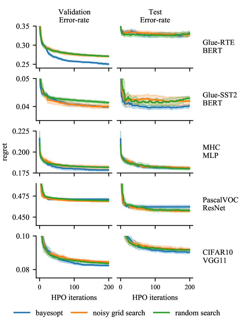
Appendix G Normality of performance distributions in the case studies
Figure G.3 presents the Shapiro-Wilk test of normality on all our results on sources of variations.
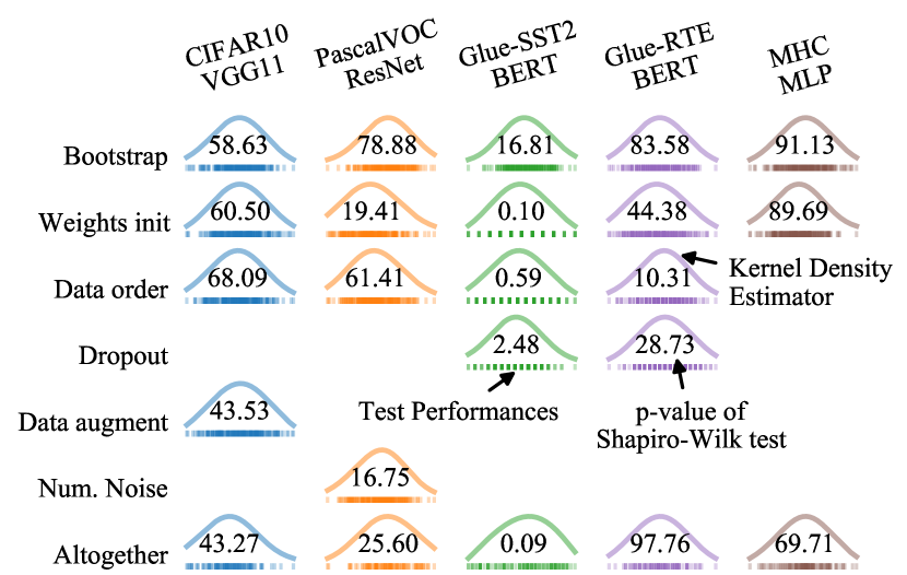
Appendix H Randomizing more sources of variance increase the quality of the estimator
Figure 5 only presented the Glue-RTE and CIFAR10 tasks. We provide here a complete picture of the standard deviation of the different estimators in Figure H.4. We further present a decomposition of the mean-squared-error in Figure H.5 to help understand why accounting for more sources of variations improves the mean-squared-error of the biased estimators.
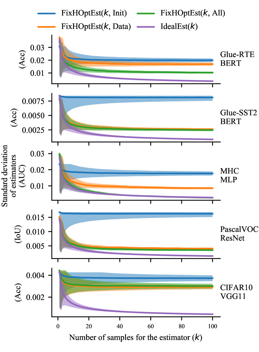
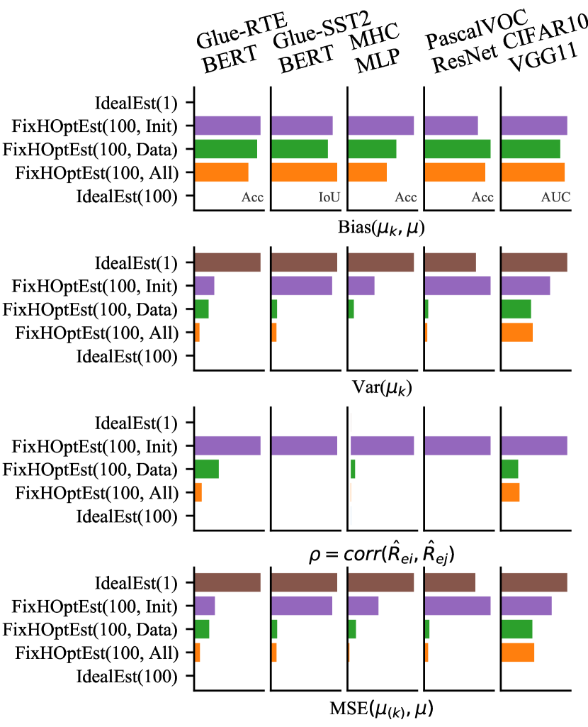
Appendix I Analysis of robustness of comparison methods
In addition to simulations described in Section 4.2, we executed experiments in which we varied the sample size and the threshold . To select the threshold of the average, we converted into the equivalent performance difference . Results are presented in Figure I.6