Abstract: Optimal design of experiments for correlated processes is an increasingly relevant and active research topic. Present methods have restricted possibilities to judge their quality. To fill this gap, we complement the virtual noise approach by a convex formulation leading to an equivalence theorem comparable to the uncorrelated case and to an algorithm giving an upper performance bound against which alternative design methods can be judged. Moreover, a method for generating exact designs follows naturally. We exclusively consider estimation problems on a finite design space with a fixed number of elements. A comparison on some classical examples from the literature as well as a real application is provided.

Key words: Correlated response; design algorithm; equivalence theorem; Gaussian processes.

Introduction and motivation

Due to its importance in spatio-temporal monitoring (cf. Mateu and Müller, 2012) and particularly computer simulation (cf. Rasmussen and Williams, 2005), experimental design for regression models with correlated errors has gained increasing interest. The theory is well developed for classical (non-)linear regression with uncorrelated errors (cf. Morris, 2010), where the corresponding optimum design approach has been initiated from Kiefer’s concept of design measures (cf. Kiefer, 1959) and has emerged into textbook status (cf. Atkinson et al., 2007, Goos and Jones, 2011, etc.). However, for the correlated setting the literature is only scattered.

The meanwhile classic approach by Sacks and Ylvisaker (1966) relied heavily on asymptotic considerations, making it valid and useful for only limited situations. In contrast, the algorithm devised by Brimkulov et al. (1980) is purely heuristic but applicable to and surprisingly efficient for a great variety of problems. The proposal of Fedorov (1996) to transform the problem into a random coefficient model allows for embedding it into standard convex design theory but requires elaborate tuning to achieve a given design size. More recently, in a remarkable series of papers started with Zhigljavsky et al. (2010), Dette, Pepelyshev and Zhigljavsky built upon and extended much of the discussions and material exposed in the pioneering monograph by Näther (1985), essentially concentrating on the ordinary least squares estimator. Latest, more promising approaches derived from the best linear unbiased estimator of the continuous-time model were proposed in Dette et al. (2016) and Dette et al. (2017).

An entirely different suggestion redefining the role of design measures was given in Pázman and Müller (1998) and fully developed in Müller and Pázman (2003). Therein a virtual noise was introduced to influence the behavior of the designs and the corresponding measure was reflecting the amount of signal suppression. The resulting procedures were quite effective, but their broader application was hampered by the downside that the method was nonconvex and thus no Kiefer-Wolfowitz-type equivalence theorem was available. In the present paper we fill this gap by asserting convexity through a new and different variant of virtual noise and consequently provide a corresponding equivalence theorem.

We will show the effectiveness of this novel modification on classical examples from the literature and compare to the above mentioned alternative techniques.

Problem description and theory

2.1 The setup

In the presentation we will constrict ourselves on linear regression models with the obvious generalizations to the asymptotic approach to the nonlinear case as outlined in Pronzato and Pázman (2013), so we assume our observations to be generated from the model

$$y\left(x\right)=f^{\mathrm{\scriptscriptstyle T}}\left(x\right)\theta+\varepsilon\left(x\right);\;\;\;x\in\mathcal{X},$$ (1)

where $\mathcal{X}=\{x_{1},\dots,x_{N}\}$ is a finite discrete design space containing $N$ points and $\theta$ is the unknown vector of parameters with dim$\left(\theta\right)=p$. What is further conventionally assumed is that the random error of the observation performed at $x$ has zero expectation, i.e. $E\left\{\varepsilon\left(x\right)\right\}=0$, and is correlated, defined through the $N\times N$ matrix $C$ with elements

$$C_{ij}=\text{cov}\,\left\{\varepsilon\left(x_{i}\right),\varepsilon\left(x_{j}\right)\right\};\quad\quad\,\,i,j=1,\ldots,N,$$

which is supposed to be known. The Gaussian process literature additionally assumes normality, which leads to the well-known kriging equations for prediction (cf. Rasmussen and Williams, 2005).

Let us now first consider an exact unreplicated $n$-point design $\mathcal{T}\subset\mathcal{X}$, where $n$ is the required number of observations. The information matrix of $\theta$ in the model (1) and for the design $\mathcal{T}$ is inversely related to the (asymptotic) variance-covariance matrix of the best linear unbiased estimator $\hat{\theta}$. As is well known, this information matrix is $M_{\mathcal{T}}=F(\mathcal{T})^{\mathrm{\scriptscriptstyle T}}C^{-1}(\mathcal{T})F(\mathcal{T})$, where $C(\mathcal{T})$ is the $n\times n$ submatrix of $C$ corresponding to points of the set $\mathcal{T}$ and $F(\mathcal{T})$ is an $n\times p$ matrix, $F_{i,j}(\mathcal{T})=f_{j}\left(x_{i}\right)$, with $x_{i}\in\mathcal{T}$ and $j=1,\ldots,p$.

The situation is quite different when the observations are uncorrelated, so that for any $x\in\mathcal{X}$ observations $y(x)$ can be replicated. Traditionally, following Kiefer (1959), we then define a design as a probability measure $\xi$ on $\mathcal{X}$, $\xi(x)$ being interpreted as to be proportional to the number of replicated observations at the design point $x$.

Typically criteria functions used for uncorrelated observations, i.e. the case of a diagonal $C$, can be expressed as concave increasing functions of the information matrix. For example, for D-optimality we have $\Phi\left(M_{\xi}\right)=\left\{\det\left(M_{\xi}\right)\right\}^{1/p}\mbox{ or }\Phi\left(M_{\xi}\right)=\log\det\left(M_{\xi}\right),$ with $M_{\xi}=\sum_{x\in\mathcal{X}}f(x)f^{\mathrm{\scriptscriptstyle T}}(x)\,\xi(x).$ It is the usual purpose of optimum design to find the design

$$\xi^{*}=\arg\max_{\xi}\Phi\left(M_{\xi}\right).$$

The maximum of $\Phi\left(M_{\xi}\right)$ over the set of all designs $\Xi$ can be obtained by convex methods. In case of strict concavity of $\Phi\left(M_{\xi}\right)$, there is only one maximum value of $M$.

It is fully justified to use in the correlated setup of model (1) the same optimality criteria functions $\Phi(M)$ as for the uncorrelated case, but now $M_{\mathcal{T}}$ should be used instead of $M_{\xi}$ (Pázman, 2007). In the method presented in this paper, we take great advantage of the fact that all statistically meaningful criteria functions $\Phi(M)$ are concave functions on the set of all symmetric positive semidefinite matrices $M$, cf. Pukelsheim (2006). Thus, we will be able to employ efficient convex optimization methods for the evaluation of approximate designs.

Note that this is usually not the case in the correlated setup, i.e. for a general $C$, where typically sophisticated non-convex optimization techniques, such as simulated annealing or particle swarms, have to be applied.

2.2 Some techniques from the literature

Such non-convex methods are for instance required for the mathematically elaborate design approaches developed by Dette, Zhigljavsky and collaborators, most recently in Dette et al. (2016) and Dette et al. (2017). There they generate their results by moving from the discretely indexed model (1) to its continuously indexed counterpart and back, thus ending up with the eventual need for discretisation and approximation of the best linear unbiased estimator. In Dette et al. (2016), they make use of the fact that the optimally-weighted signed least squares estimator has the same variance as the best linear unbiased estimator. They derive the weight function of the signed least squares estimator for the continuous model and regard this as the design measure. In Dette et al. (2017), they propose an approximate criterion based on a discrete approximation of the best linear unbiased estimator for the continuous model. The approximate criterion needs to be optimized numerically in the same way as the original criterion, so there is no major conceptual difference when it comes to optimization with the exception of the former being computationally more efficient if $p<<n$. Therefore, in the following we shall not consider these approximate criteria, as Dette et al. (2017) have already investigated how good/bad this approximation works.

Limitations of the methods of Dette et al. (2016) and Dette et al. (2017) are that they are constrained to a limited form of covariance kernels and that it may be quite difficult to generalize to higher-dimensional design spaces.

In contrast, the suggestion by Fedorov (1996) is to approximate directly the error component through Mercer’s covariance expansion of degree $q$, i.e. $\sum_{l=1}^{q}\gamma_{l}\varphi_{l}(x)$, where the $\varphi_{l}(x)$ and $\lambda_{l}$ are the eigenfunctions and eigenvalues, respectively, of the covariance kernel. This leads to model (1) being approximated by a mixed (random and fixed) coefficient regression model and allows for embedding into standard convex design theory, albeit involving a potentially high number of $q$ additional regressors and corresponding inflation of the information matrix plus some arbitrariness in determining an appropriate $q$. Incidentally it was shown in Pázman and Müller (2010) that for a finite setup the method can be embedded into techniques similar to the one described in the next subsection with very specific variances of the virtual noise components.

The most straightforward and pragmatic approach, however, is the greedy algorithm for exact design generation first proposed by Brimkulov et al. (1980), in the modification and interpretation given in Fedorov (1996). There the so-called sensitivity function of the classical one-point correction algorithms for D-optimality in the uncorrelated setup is used with expressions simply replaced by their analogues from the correlated case. That is, at each step $r$ we augment the point

$$x_{r}=\arg\max_{\mathcal{X}}f^{\mathrm{\scriptscriptstyle T}}(x)M^{-1}_{\mathcal{T}_{r-1}}f(x)/\sigma^{2}_{\varepsilon}(x)$$

to the current design $\mathcal{T}_{r-1}\subset\mathcal{T}$, with $f$, $M$, and the error variance $\sigma^{2}_{\varepsilon}$ replaced accordingly, see the appendix for details. Furthermore, the appendix contains an adaption for A-optimality, which will be utilized in some of the examples. Note that despite its compellingly simple form, this algorithm has little theoretical basis other than that the independent case can be seen as a particular limit instance of the general setup.

A good overview of all these approaches with an application in spatio-temporal sensor placement, albeit mainly from the perspective of using the ordinary least squares estimator, can most recently be found in Uciński (2020).

2.3 Virtual noise

In this paper, we will use a technique that has first been proposed in Pázman and Müller (1998), which is very different from the above. Despite a certain similarity to the standard kriging setup, in that we consider two error components, one correlated and the other uncorrelated, our additional uncorrelated error component however is not considered as an observational error but as a regulatory device without physical meaning, termed virtual noise. The purpose of this noise is to suppress the signal whenever the design measure is small relative to the maximum value of the design measure. To make this operational, the variance of this virtual noise needs to be assumed being of a specific form. Unfortunately the specifications given in Pázman and Müller (1998) as well as in Müller and Pázman (2003) both yielded a nonconvex solution. In this paper, we intend to fill this gap by providing convexity and consequently an equivalence theorem that allows for quick checks of whether particular designs optimize the design criterion as well as an algorithm to find the optimum.

First, similarly as in Müller and Pázman (2003), define a convex set of restricted probability measures, also termed design measures or simply designs,

$$\Xi=\left\{\xi:\sum_{x\in\mathcal{X}}\xi\left(x\right)=1,\>\forall_{x\in\mathcal{X}}\>0~{}\leq~{}\xi\left(x\right)\leq 1/n\right\},$$

on the design space $\mathcal{X}$, which is supposed to be finite. The integer number $n$ represents the desired number of points of support of an optimum exact design $\xi^{*}$. Now instead of (1), consider the potentially perturbed variables

$$y\left(x\right)=f^{\mathrm{\scriptscriptstyle T}}\left(x\right)\theta+\varepsilon\left(x\right)+w_{\xi}\left(x\right);\;\;\;x\in\mathcal{X},$$ (2)

where the variance of the supplementary ’virtual noise’ $w_{\xi}$, independent of $\varepsilon$, is fixed as

$$\text{var}\,\left\{w_{\xi}\left(x\right)\right\}=\sigma^{2}_{\xi}(x)=\kappa\frac{1/n-\xi\left(x\right)}{\xi\left(x\right)},$$

whereas $\text{cov}\,\left\{w_{\xi}\left(x\right),w_{\xi}\left(x^{\prime}\right)\right\}=0\text{ when }x\neq x^{\prime}.$ The positive number $\kappa$ is a tuning parameter which must be chosen within the bounds given by Theorem 1 and should be taken as large as possible to emphasize the influence of the virtual noise. The experience obtained in the examples below is that a smaller choice of $\kappa$ diminishes mainly the speed of the linear programming algorithm from Section 2.4.

That means, similarly as in Müller and Pázman (2003), if $\xi\left(x\right)=0$, i.e. $\sigma^{2}_{\xi}=\infty$, there is no observation at the point $x$, and if $\xi\left(x\right)=1/n$, i.e. $\sigma^{2}_{\xi}=0$, the observation at the point $x$ is not disturbed at all by the virtual noise.

An important notion is the concept of an exact $k$-point design, for which in our context we require a slightly different definition as usual. Here, it is a design $\xi\in\Xi$ for which the signal is not disturbed by the virtual noise in the $k$ points $x_{1},\ldots,x_{k}\in\mathcal{X}$, i.e. $\xi(x_{i})=1/n$, and the signal is totally suppressed in all other points, i.e. $\xi(x)=0\;\>\forall\>x\in\mathcal{X}\backslash\{x_{1},\ldots,x_{k}\}$. It follows trivially from the definition of $\Xi$ that all $n$-point exact designs are in $\Xi$, but $\Xi$ contains no $k$-point exact designs with $k\neq n$. The set $\Xi$ has also another property: it is the smallest closed convex set of probability measures on $\mathcal{X}$ which contains all $n$-point exact designs. The primary aim of the statistician is to consider exact $n$-point designs, so the set $\Xi$ is the smallest possible convex extension of the set of such exact designs.

In the proofs we shall also require the set

$$\Xi_{+}=\left\{\xi:\sum_{x\in\mathcal{X}}\xi(x)=1,\>\forall_{x\in\mathcal{X}}\>0<\xi(x)\leq 1/n\right\}=\left\{\xi\in\Xi:\>\text{supp}(\xi)=\mathcal{X}\right\}.$$

Its advantage is that $\text{var}\,\left\{w_{\xi}\left(x\right)\right\}<\infty$ for every $x\in\mathcal{X}$, $\xi\in\Xi_{+}$. One can easily see that $\Xi$ is the closure of $\Xi_{+}$.

Denote by $W\left(\xi\right)$ the $N\times N$ diagonal matrix

$$W_{i,j}\left(\xi\right) = \kappa\frac{1/n-\xi\left(x_{i}\right)}{\xi\left(x_{i}\right)};\mbox{ if }\,\,\,i=j$$

$$= 0;\qquad\qquad\quad\>\>\mbox{ if }\,\,i\neq j.$$

When $\xi\in\Xi_{+}$, i.e. $\text{supp}(\xi)=\mathcal{X}$, the information matrix of $\theta$ in model (2) is given by

$$M(\xi)=F^{\mathrm{\scriptscriptstyle T}}\left\{C+W\left(\xi\right)\right\}^{-1}F,$$ (3)

where $C$ is the $N\times N$ covariance matrix defined after (1), and $F$ is the $N\times p$ matrix $F_{i,j}=f_{j}(x_{i}),\>x_{i}\in\mathcal{X},\>i=1,\ldots,N,\>j=1,\ldots,p$. Evidently, $M(\xi)$ is nonsingular if $F$ has full rank $p$.

On the other hand, when $\xi\in\Xi\backslash\Xi_{+}$, we define

$$M(\xi)=F^{\prime\mathrm{\scriptscriptstyle T}}\left\{C^{\prime}+W^{\prime}\left(\xi\right)\right\}^{-1}F^{\prime},$$ (4)

where $C^{\prime}$, $W^{\prime}(\xi)$ are submatrices of $C$, $W(\xi)$ restricted to the support $\text{supp}(\xi)$, and similarly are the rows of $F^{\prime}$. An important property is the continuity of $M(\xi$) on the whole set $\Xi$, i.e. $\xi_{n}(x)\to\xi(x)$ for every $x\in\mathcal{X}$ implies $M(\xi_{n})\to M(\xi)$, see Lemma A2 in the appendix.

Another interesting property of $M(\xi)$ is that in case of uncorrelated observations with constant variances, $C=\sigma^{2}I$, with $\kappa=\sigma^{2}$ we obtain $M(\xi)=M_{\xi}$, the information matrix from Kiefer’s design theory. However, for general $C$ the design measure can no more be interpreted as reflecting the replications of observations. In any case we can still use it to obtain heuristically exact $n$-point designs approaching the quality of an optimum exact design as will be demonstrated in the examples section.

We now have the following

Theorem 1.

If $\kappa<\lambda_{\min}\left(C\right),$ the minimal eigenvalue of the matrix $C,$ and if $\Phi\left(M\right)$ is any optimality criterion expressed as a concave, increasing, and continuous function of the matrix $M$, then the mapping

$$\xi\in\Xi\rightarrow\Phi\left\{M(\xi)\right\}$$

is concave as well, with $M(\xi)$ defined in $\left(\ref{FIMvirtual}\right)$ and $\left(\ref{FIMvirtual2}\right)$.

The proof of the theorem is given in the appendix. Its consequences are that the maximum of $\Phi(M)$ over the set $\Xi$ can be obtained by convex methods, and in case of a strict concavity of $\Phi(M)$, there is only one optimal $M$.

Unfortunately however, the gradient method so popular in uncorrelated observations cannot be used here because one-point design measures do not enter into the set $\Xi$. Neither can we use the usual equivalence theorem, which requires the use of one-point designs as well. However, the methods of modified linear programming can be employed, see the next subsection, and also a certain form of the equivalence theorem can be provided, which is given in Section 2.5.

2.4 A design algorithm

The method used in this subsection originated as the cutting-plane method of Kelley (1960), was then adapted to experimental design in Chapter 9 of Pronzato and Pázman (2013) and applied algorithmically to classical experimental design in Burclová and Pázman (2016).

For computational reasons we shall restrict our attention in this section to the set

$$\Xi^{\epsilon}=\left\{\xi\in\Xi:\>\forall_{x\in\mathcal{X}}\>\xi(x)\geq\epsilon\right\}$$

for some small $\epsilon>0$. Evidently,

$$\Xi_{+}=\bigcup_{\epsilon>0}\Xi^{\epsilon}.$$

Since the closure of $\Xi_{+}$ is the set $\Xi$ and since according to Lemma A2 in the appendix the criterion function $\Phi\left\{M(\xi)\right\}$ is continuous on the whole of $\Xi$, we can approach the value of $\max_{\xi\in\Xi}\Phi\left\{M(\xi)\right\}$ arbitrarily close by computing $\Phi\left\{M(\xi^{*}_{\epsilon})\right\}$, where $\xi^{*}_{\epsilon}\in\arg\max_{\xi\in\Xi^{\epsilon}}\Phi\left\{M(\xi)\right\}$.

If $\Phi(M)$ is a global criterion, like $D-$ or $A-$optimality, which has a gradient $\nabla_{M}\Phi(M),$ then for any $\xi$ in $\Xi_{+}=\{\xi\in\Xi:\text{supp}(\xi)=\mathcal{X}\}$ we have the derivative

$$\frac{\partial\Phi\left\{M(\xi)\right\}}{\partial\xi(\bar{x})}=\text{tr}\left[\nabla_{M}\Phi\left\{M(\xi)\right\}\,\,\frac{\partial M(\xi)}{\,\,\,\partial\xi(\bar{x})}\right],$$

where $\nabla_{M}\Phi\left\{M(\xi)\right\}$ denotes $\nabla_{M}\Phi(M)$ at $M=M(\xi)$. The linear Taylor formula for $\xi\rightarrow\Phi\left\{M(\xi)\right\}$ at the point $\mu$ gives

$$\Phi\left\{M(\mu)\right\}+\sum_{\bar{x}\in\mathcal{X}}\text{tr}\left[\nabla_{M}\Phi\left\{M(\mu)\right\}\,\,\frac{\partial M(\mu)}{\,\,\,\partial\mu(\bar{x})}\right]\left\{\xi(\bar{x})-\mu(\bar{x})\right\},$$ (5)

which is linear in $\xi$, so due to the concavity, we have for any $\xi\in\Xi^{\epsilon}$

$$\Phi\left\{M\left(\xi\right)\right\}=\min_{\mu\in\Xi^{\epsilon}}\left(\Phi\left\{M(\mu)\right\}+\sum_{\bar{x}\in\mathcal{X}}\text{tr}\left[\nabla_{M}\Phi\left\{M(\mu)\right\}\,\,\frac{\partial M(\mu)}{\,\,\,\partial\mu(\bar{x})}\right]\left\{\xi(\bar{x})-\mu(\bar{x})\right\}\right)$$ (6)

and $\arg\max_{\xi}\Phi\{M(\xi)\}$ is the optimal design on $\Xi^{\epsilon}$. It follows that for a differentiable positive criterion function $\Phi$ the optimal design problem is an “infinite-dimensional linear programming problem”, which can be solved iteratively.

To see the details, let us take a look at the particular specification for D-optimality. Take $\Phi(M)=\left\{\det(M)\right\}^{1/p}$. Then for any nonsingular $M$

$$\nabla_{M}\Phi(M)=M^{-1}\cdot p^{-1}\left\{\det(M)\right\}^{1/p}.$$

According to (3), supposing that $F$ has full rank we have that $M^{-1}(\mu)$ exists for any $\mu\in\Xi_{+}$, and we also have

$$\frac{\partial M(\mu)}{\,\,\,\partial\mu(\bar{x})}=\frac{\kappa}{n}F^{\mathrm{\scriptscriptstyle T}}H^{-1}(\mu)\Gamma\left\{\mu^{-2}(\bar{x})\right\}H^{-1}(\mu)F,$$

with

$$H(\mu)=\left[\left(C-\kappa I\right)+\frac{\kappa}{n}\,\text{diag}\left\{\mu^{-1}(\cdot)\right\}\right],$$

where $\text{diag}\left\{\mu^{-1}(\cdot)\right\}$ is an $N\times N$ diagonal matrix with $\mu^{-1}(x)$ as diagonal elements, and $\Gamma\left\{\mu^{-2}(\bar{x})\right\}$ is an $N\times N$ matrix having zero elements everywhere up to the $\bar{x}$th diagonal position, where we have $\mu^{-2}(\bar{x})$. Thus, the expression (5) becomes

$$\left[\det\left\{F^{\mathrm{\scriptscriptstyle T}}H^{-1}(\mu)F\right\}\right]^{1/p}\times$$

$$\times\left[1+\frac{\kappa}{np}\sum_{\bar{x}\in\mathcal{X}}\left\{H^{-1}(\mu)\right\}_{\bar{x},.}F\left\{F^{\mathrm{\scriptscriptstyle T}}H^{-1}(\mu)F\right\}^{-1}F^{\mathrm{\scriptscriptstyle T}}\left\{H^{-1}(\mu)\right\}_{.,\bar{x}}\frac{\xi(\bar{x})-\mu(\bar{x})}{\mu^{2}(\bar{x})}\right].$$

Returning to the general case, we can now reformulate the design problem into a linear program. Any concave and positive criterion

$$\xi\in\Xi^{\epsilon}\rightarrow\Phi\left\{M(\xi)\right\}$$

can be written in a form

$$\Phi\left\{M(\xi)\right\}=\min_{\mu\in\Xi^{\epsilon}}\left\{a(\mu)+\sum_{i=1}^{N}b_{i}(\mu)\,\xi(x_{i})\right\}.$$

Here, $a(\mu)$ and $b_{i}(\mu)$ can be obtained either from the linear Taylor formula (6), or, in case that there is no gradient, from subgradients, or using some algebraic tricks as in Burclová and Pázman (2016).

At the first step of the linear program, we set a finite set $\Xi_{1}\subset\Xi^{\epsilon}$, which will be increased in the later steps. Hence, at the $k$th step we start with a set $\Xi_{k}$. Consider the following finite set of constraints, which are linear in the variables $t\in\mathbb{R}$ and $\xi(x);\>x\in\mathcal{X}$,

$$t \geq 0,\qquad t\leq a(\mu)+\sum_{i=1}^{N}b_{i}(\mu)\,\xi(x_{i})\text{,\thinspace\thinspace\thinspace\thinspace\thinspace}\mu\in\Xi_{k};$$

$$\xi(x_{i}) \geq \epsilon;\qquad\xi(x_{i})\leq\frac{1}{n};\quad\quad i=1,\dots,N,\qquad\sum_{i=1}^{N}\xi(x_{i})=1,$$

and consider a standard linear program which maximizes $t$ under these constraints. Denote $t^{\left(k\right)}$ and $\xi^{\left(k\right)}$ those values of $t$ and of $\xi$ where the maximum of $t$ is attained. Define $\Xi_{k+1}=\Xi_{k}\cup\left\{\xi^{(k)}\right\}$ and repeat the linear program with $\Xi_{k+1}$ instead of $\Xi_{k}$.

To make this operational, we also require a stopping rule. We have that

$$t^{\left(k\right)} = \max_{\xi\in\Xi^{\epsilon}}\min_{\mu\in\Xi_{k}}\left\{a(\mu)+\sum_{i=1}^{N}b_{i}(\mu)\,\xi(x_{i})\right\}$$

$$\geq \max_{\xi\in\Xi^{\epsilon}}\min_{\mu\in\Xi^{\epsilon}}\left\{a(\mu)+\sum_{i=1}^{N}b_{i}(\mu)\,\xi(x_{i})\right\}$$

$$= \max_{\xi\in\Xi^{\epsilon}}\,\Phi\left\{M(\xi)\right\}\geq\max_{\xi\in\Xi_{k}}\Phi\left\{M(\xi)\right\}.$$

Hence, if we have a small number $\delta>0$, such that $t^{\left(k\right)}-\max_{\xi\in\Xi_{k}}\Phi\left\{M(\xi)\right\}<\delta,$ then

$$\max_{\xi\in\Xi_{k}}\Phi\left\{M(\xi)\right\}>\max_{\xi\in\Xi^{\epsilon}}\,\Phi\left\{M(\xi)\right\}-\delta$$

and $\arg\max_{\xi\in\Xi_{k}}\Phi\left\{M(\xi)\right\}$ is the nearly optimum design. Evidently, $\max_{\xi\in\Xi_{k}}\Phi\left\{M(\xi)\right\}$ can be simply computed iteratively,

$$\max_{\xi\in\Xi_{k}}\Phi\left\{M(\xi)\right\}=\max\left[\max_{\xi\in\Xi_{k-1}}\Phi\left\{M(\xi)\right\},\,\,\Phi\left\{M\left(\xi^{\left(k\right)}\right)\right\}\right].$$

2.5 Equivalence theorem

In this section, we shall consider only global optimality criteria having a gradient $\nabla_{M}\Phi(M)$ such as the D- and A-criterion. We shall use an abbreviated notation writing

$$h\left(x,{\xi}\right)=\left\{T\left({\xi}\right)\right\}_{x,.}G\left({\xi}\right)\left\{T^{\mathrm{\scriptscriptstyle T}}\left({\xi}\right)\right\}_{.,x},$$

where

$$G(\xi) = F\left[\nabla_{M}\Phi\left\{M(\xi)\right\}\right]F^{\mathrm{\scriptscriptstyle T}},$$

$$T(\xi) = \left[\left(C-\kappa I\right)\,\,\text{diag}\left\{\xi(\cdot)\right\}+\frac{\kappa}{n}I\right]^{-1}.$$

Theorem 2.

Let $\Phi$ be a global, concave and nonnegative optimality criterion, zero on singular matrices, and having a gradient. A design measure $\bar{\xi}\in\Xi$ with a nonsingular $M\left(\bar{\xi}\right)$ is $\Phi-$optimal (within our theory) if and only if for every n-tuple $z_{1},\ldots,z_{n}$ of points from $\mathcal{X}$ we have

$$\frac{1}{n}\sum_{i=1}^{n}h(z_{i},\bar{\xi})\leq\sum_{x\in\mathcal{X}}\bar{\xi}(x)h(x,\bar{\xi}).$$ (7)

Moreover, if $\bar{\xi}$ satisfies the inequality

$$\frac{1}{n}\sum_{i=1}^{n}h(z_{i},\bar{\xi})\leq\sum_{x\in\mathcal{X}}\bar{\xi}(x)h(x,\bar{\xi})+\delta$$ (8)

for some $\delta>0$ and any $z_{1},\dots,z_{n}\in\mathcal{X}$, we have that

$$\Phi\{M(\bar{\xi})\}\geq\max_{\xi\in\Xi}\Phi\{M(\xi)\}-\delta.$$ (9)

The full proof is given in the appendix.

Remark 1.

The numerical exploitation of this theorem is straightforward:

For a fixed design $\bar{\xi}\in\Xi$ and for any $x\in\mathcal{X}$ compute the number $h\!\left(x,\bar{\xi}\right)$ and compute the sum $d\!\left(\bar{\xi}\right)=n\sum_{x\in\mathcal{X}}\bar{\xi}(x)\,h\!\left(x,\bar{\xi}\right)$. Order the points of the set $\mathcal{X}$ so that $h\!\left(x_{1},\bar{\xi}\right)\geq\cdots\geq h\!\left(x_{N},\bar{\xi}\right)$. Then (7) is equivalent to the inequality

$$\sum_{i=1}^{n}h\!\left(x_{i},\bar{\xi}\right)\leq d\!\left(\bar{\xi}\right),$$

and (8) is equivalent to the inequality

$$\sum_{i=1}^{n}h\!\left(x_{i},\bar{\xi}\right)\leq d\!\left(\bar{\xi}\right)+n\delta.$$

Note that the possibility to formulate an equivalence theorem due to concavity means that we can provide a rather close upper bound for the performance of all exact $n$-point designs. Thus we can calibrate the performance of all existing methods by this bound, as will be done in the next section.

Examples

3.1 General considerations

To check our ideas, we have computed designs for numerous examples from the literature, particularly those already presented and compared in Glatzer and Müller (1999). In most of these examples, all compared methods did reasonably well, so for illustration we have just selected four, which we consider representative and for which we give details below.

The ultimate goal in all our examples is to find an exact design and to judge its quality. As for all measure-based design approaches, we therefore require a method to convert the calculated measure to a discrete set of points. Dette et al. (2016) typically use the endpoints plus quantiles of their measure in their one-dimensional examples. We will thus for comparison purposes use the same method for our approach, but there is no simple way to extend this to higher dimensions. Instead, in the spirit of the random design strategies defined in Waite and Woods (2020), one can perform random sampling according to the measure multiple times and select the sampled design with the best criterion value. We will denote this approach by R-VN (random sampling virtual noise). In our experience, this strategy has led to even more efficient designs in all cases, and we apply this approach using 100 samples whenever the design dimension is greater than one. We furthermore provide the results for the one-dimensional cases in the appendix, which also contains some additional examples.

In the following examples, we will compare our method based on the optimal measure for the virtual noise representation to the method from Dette et al. (2016) as well as to the variant of the algorithm of Brimkulov et al. (1980) put forward by Fedorov (1996) based on approximate sensitivity functions, henceforth denoted by BKSF. An algorithmic description of the latter can be found in the appendix. We refrain from reporting results from the original algorithm which is tantamount to an exchange method based on direct comparisons of criterion values, as most of the time they gave very similar results. For comparison purposes, we also provide the median performance out of 100 randomly chosen exact designs of the respective size and denote this approach by R-UNIF.

As Dette et al. (2016), we only consider examples with one design variable. For all methods except the one from Dette et al. (2016), the design space to search over was discretized to a $101$-point design grid. For small $n$ we performed an exhaustive search of all $n$-point combinations over the design grid to obtain the true optimum exact design. We report those points in the tables as well, where we abbreviate this approach by EXS (exhaustive search). We consider two different ways how to obtain the exact $n$-point designs for our method. The first is to select the quantiles $1/(n+1),\ldots,n/(n+1)$ of the design grid with respect to the design measure. The second way is to always include the endpoints of the design grid and select the quantiles $1/(n-1),\ldots,(n-2)/(n-1)$ of the remaining mass over the design grid. We denote these two methods by Q-VN and Q-VN+EP (quantile virtual noise plus endpoints), respectively. The second approach is similar to the approach of Dette et al. (2016), which we will denote by Q-DPZ+EP. The design measures Dette et al. (2016) consider usually have discrete masses at the endpoints but are continuous elsewhere, so Dette et al. (2016) always include the endpoints and select the quantiles for the design points in between with respect to the continuous measure.

From Theorem 2 it follows that $\Phi\left(M_{\mathcal{T}}\right)$ for any $n$-point exact design $\mathcal{T}$ is bounded from above by $\Phi\left\{M\!\left(\bar{\xi}\right)\right\}$ for the $\Phi$-optimal design measure $\bar{\xi}$, where $M(\xi)$ is given by (3). Therefore, we report the efficiencies with respect to $\Phi\left\{M\!\left(\bar{\xi}\right)\right\}$, where $\bar{\xi}$ is found by applying the linear programming algorithm. Let $\Xi_{k}$ be the finite set of design measures determining the set of linear constraints in step $k$ of the linear programming algorithm and let

$$t^{\left(k\right)}=\max_{\xi\in\Xi^{\epsilon}}\min_{\mu\in\Xi_{k}}\left\{a(\mu)+\sum_{i=1}^{N}b_{i}(\mu)\,\xi(x_{i})\right\},$$

see Section 2.4. Denote $\Phi^{(k)}=\max_{\xi\in\Xi_{k}}\Phi\left\{M(\xi)\right\}$. In our programs, we stop the linear programming algorithm if $\frac{t^{(k)}-\Phi^{(k)}}{\Phi^{(k)}}\leq 10^{-4}.$ We set $\epsilon=10^{-6}$ in all our examples to avoid numerical problems. To solve the linear programming problems, we use the package lpSolve (Berkelaar et al., 2020) from the software R (R Core Team, 2020). In all our examples we also choose $\kappa$ to be rounded down from $\lambda_{min}(C)$ to two significant digits.

In all the figures we present, the left panel displays the discrete measure obtained by running the linear programming algorithm for the virtual noise representation for a particular $n$. The right panel shows the D-efficiencies of exact designs obtained by various methods up to $n=20$. The methods depicted are: Q-VN (solid red line with squares), Q-VN+EP (dashed green line with large dots), Q-DPZ+EP (long-dashed blue line with triangles), BKSF (dotted black line with diamonds), and reporting the median efficiency for R-UNIF (long-short-dashed grey line with small dots).

3.2 Example 1: a classic one-parameter model

This example has originally been considered by Sacks and Ylvisaker (1966). Dette et al. (2016) use it to illustrate the efficiency of their method. It is a one-parameter model given by

$$f(x) = 1+0.5\sin(2\pi x),\qquad x\in[1,2],$$

$$\text{cov}\,\{\varepsilon(x),\varepsilon(x^{\prime})\} = \begin{cases}x^{2}x^{\prime}\qquad x\leq x^{\prime}\\ x(x^{\prime})^{2}\quad x>x^{\prime},\end{cases}\quad\lambda_{\min}(C)=0.00276.$$

For the D-criterion and $n=4$, the selected design points and D-efficiencies for the various methods are given in Table 1. While the algorithm using the approximate sensitivity function from Fedorov (1996) comes close to the result of the exhaustive search and to $90\%$ of the upper bound, the measure-based methods are considerably worse. However, when we increase the sample size (see Fig. 1), their performance improves and slowly approaches the bound.

Table 1: Optimal designs and D-efficiencies for Example 1

	$x_{1}$	$x_{2}$	$x_{3}$	$x_{4}$	D-eff
Q-VN	1.10	1.23	1.40	1.76	0.8316
Q-VN+EP	1.00	1.21	1.58	2.00	0.7865
Q-DPZ+EP	1.00	1.28	1.69	2.00	0.8455
R-UNIF					0.6955
BKSF	1.19	1.67	1.79	2.00	0.9075
EXS	1.22	1.66	1.79	2.00	0.9158

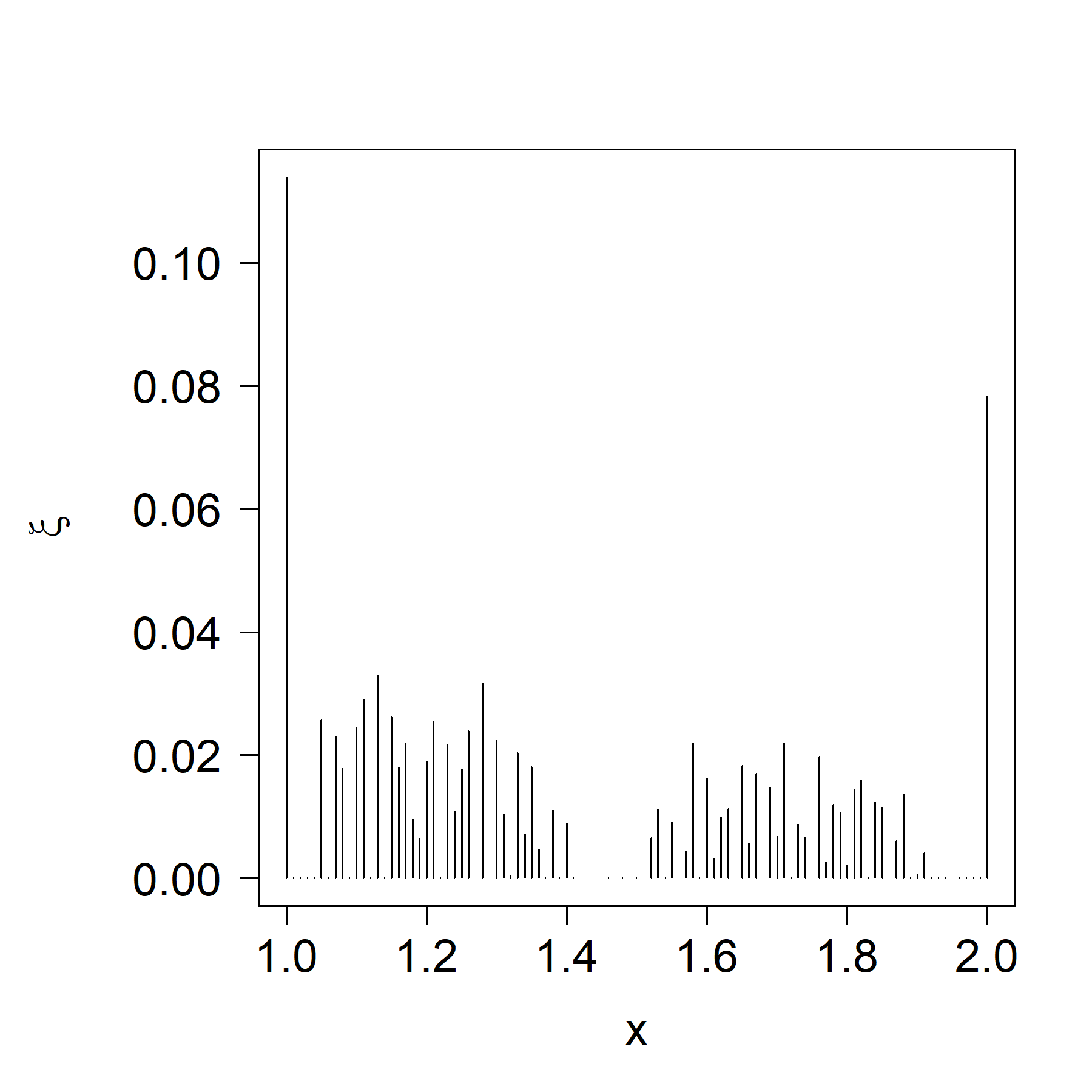
Figure 1: Our measure (left panel) and efficiencies (based on our bound) versus sample size (right panel) for Example 1.

Note that in contrast to the method by Dette et al. (2016) our method does not require the existence of the continuous best linear unbiased estimator. To illustrate this, we modify the example by using the kernel $\text{cov}\,\{\varepsilon(x),\varepsilon(x^{\prime})\}=\min(x,x^{\prime})^{2}\left\{3\max(x,x^{\prime})-\min(x,x^{\prime})\right\}/6$ instead, which is the once continuously differentiable kernel for the integrated Brownian motion error process. According to Dette et al. (2019), the continuous best linear unbiased estimator therefore has to incorporate information from the first derivatives of the error process to be estimable. Since this kernel is now much smoother, the minimum eigenvalue for our design grid is rather small, namely $\lambda_{\min}(C)=2.0854\cdot 10^{-8}$. However, we did not observe any numerical issues due to that fact.

Table 2: Optimal designs and D-efficiencies for the modified Example 1

	$x_{1}$	$x_{2}$	$x_{3}$	$x_{4}$	D-eff
Q-VN	1.00	1.01	1.39	1.53	0.4933
Q-VN+EP	1.00	1.22	1.53	2.00	0.7329
R-UNIF					0.4887
BKSF	1.00	1.39	1.80	2.00	0.8042
EXS	1.00	1.23	1.75	2.00	0.9715

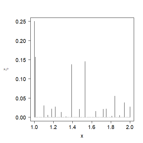
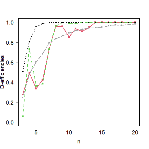
Figure 2: Our measure (left panel) and efficiencies versus sample size (right panel) for the modified Example 1.

Our algorithm puts a high amount of mass at the two lowest points in the design grid, see Figure 2. This can be interpreted as the algorithm trying to obtain information about the first derivative at the lower bound.

3.3 Example 2: a multiparameter case

The next example is taken from Section 3.6 of Dette et al. (2016). The specifications of this four-parameter model are

$$f^{\mathrm{\scriptscriptstyle T}}(x) = \left(1,x,x^{2},x^{3}\right),\quad x\in[1,2],$$

$$\text{cov}\,\{\varepsilon(x),\varepsilon(x^{\prime})\} = \min\left(x,x^{\prime}\right),\qquad\lambda_{\min}(C)=0.0025.$$

We again consider the D-criterion, so for $n=5$, Table 7 contains the selected design points and D-efficiencies. This is one of the rare cases in which our method does even slightly better than the algorithm using the approximate sensitivity function from Fedorov (1996). All methods provide considerable improvements over uniform random designs.

Table 3: Optimal designs and D-efficiencies for Example 2

	$x_{1}$	$x_{2}$	$x_{3}$	$x_{4}$	$x_{5}$	D-eff
Q-VN	1.00	1.16	1.52	1.84	2.00	0.9251
Q-VN+EP	1.00	1.20	1.52	1.82	2.00	0.9300
Q-DPZ+EP	1.00	1.14	1.33	1.60	2.00	0.8554
R-UNIF						0.3208
BKSF	1.00	1.16	1.46	1.83	2.00	0.9270
EXS	1.00	1.21	1.61	1.84	2.00	0.9308

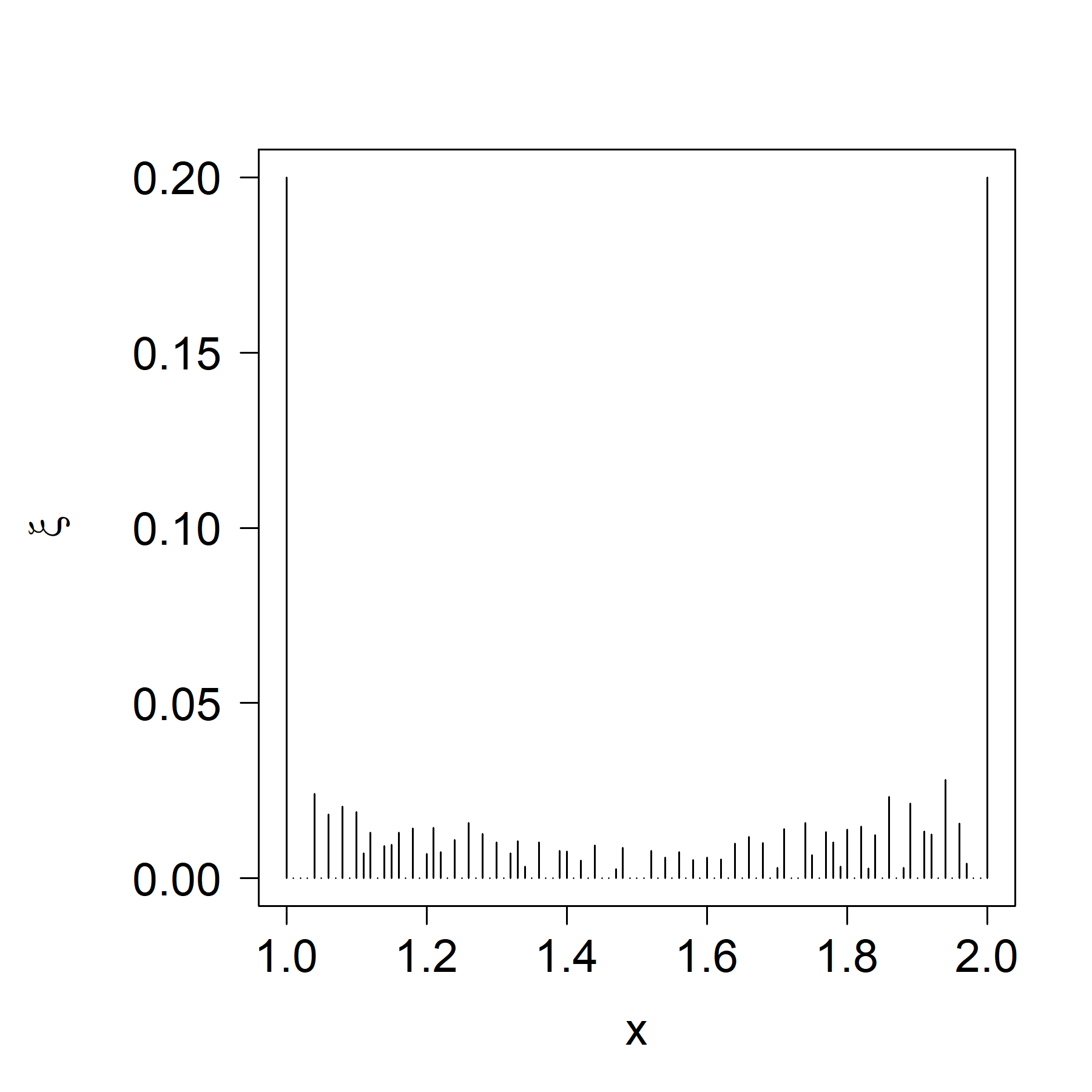
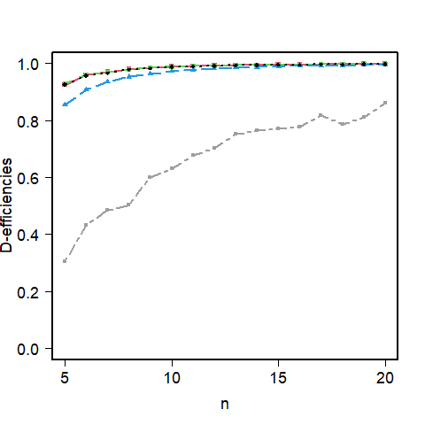
Figure 3: Our measure (left panel) and efficiencies versus sample size (right panel) for Example 2.

3.4 Example 3: a real application

We consider a real-world application inspired by the example used throughout Mateu and Müller (2012). There a dataset with temperature and rainfall measurements gathered from 37 weather stations in the Austrian state of Upper Austria during the years 1994 – 2009 was considered. Given this information, the goal was to find optimal designs for adding or reorganizing stations to optimize various aspects of future data collection.

As for Figure 1.4 of Mateu and Müller (2012) we employ the rainfall data from July 1994 and obtain the kriging estimates for an exponential kernel. The response function is assumed to be a plane, that is, it is linear in the coordinates. For our example, we assume that the parameters of the kernel function are known and set them to the kriging estimates. The model we consider is therefore

$$f^{\mathrm{\scriptscriptstyle T}}(x) = \left(1,x_{1},x_{2}\right),\qquad x=(x_{1},x_{2})^{\mathrm{\scriptscriptstyle T}},$$

$$\text{cov}\,\{\varepsilon(x),\varepsilon(x^{\prime})\} = 1756.65\cdot\exp\left(\left\|x-x^{\prime}\right\|_{2}\bigl{/}40792.35\right).$$

The design set is composed of the centroids of the $N=445$ Upper Austrian municipalities, for which $\lambda_{\min}(C)=42.15$. We set $n=36$ because this was the number of active weather stations in July 1994. Our hypothetical objective is therefore to reorganize the whole weather station network in order to most efficiently estimate the response function parameters given the assumed kernel function. We use the D-criterion as in the previous examples.

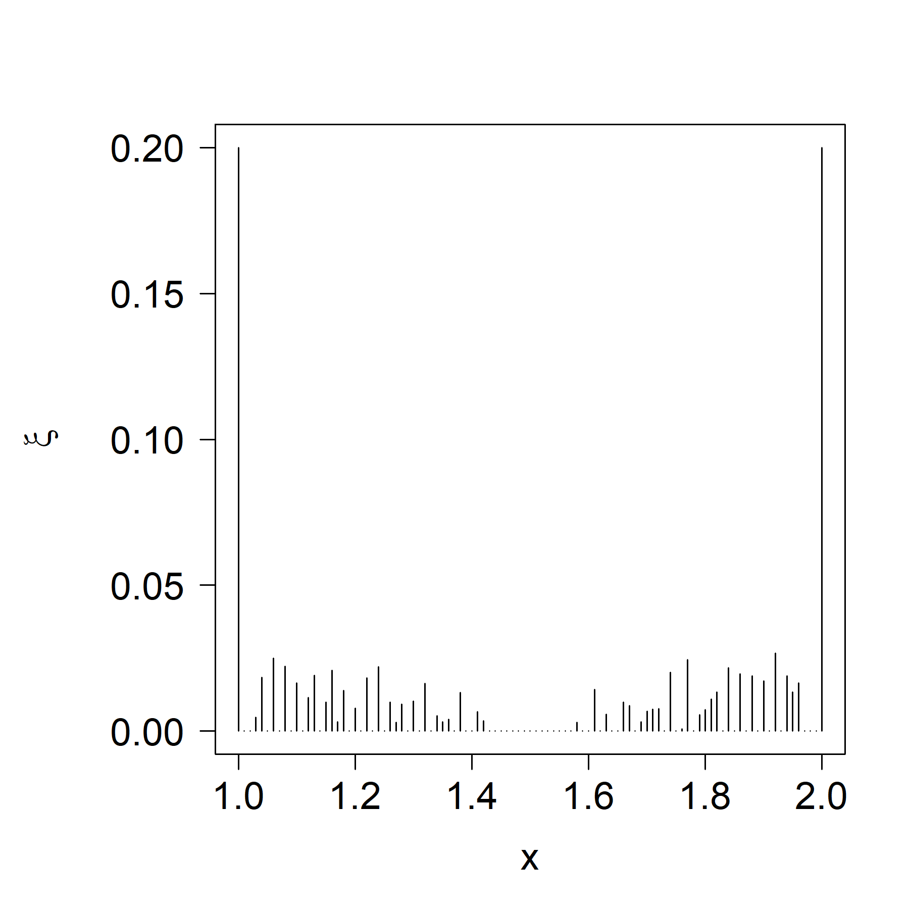
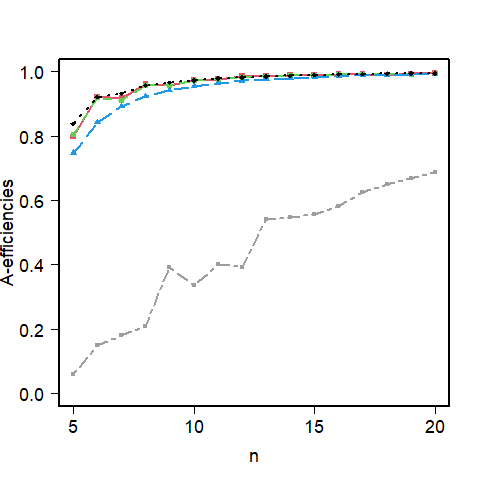
Figure 5: Our measure (left panel) and efficiencies versus sample size (right panel) for the modified Example 4.

The left panel of Figure 5 displays the optimal measure obtained for the virtual noise representation when $n=36$. The majority of the mass is concentrated on the borders. The right panel shows the optimal 36-point design we obtain by selecting the design with the highest criterion value out of 100 random designs sampled according to the measure depicted in the left panel.

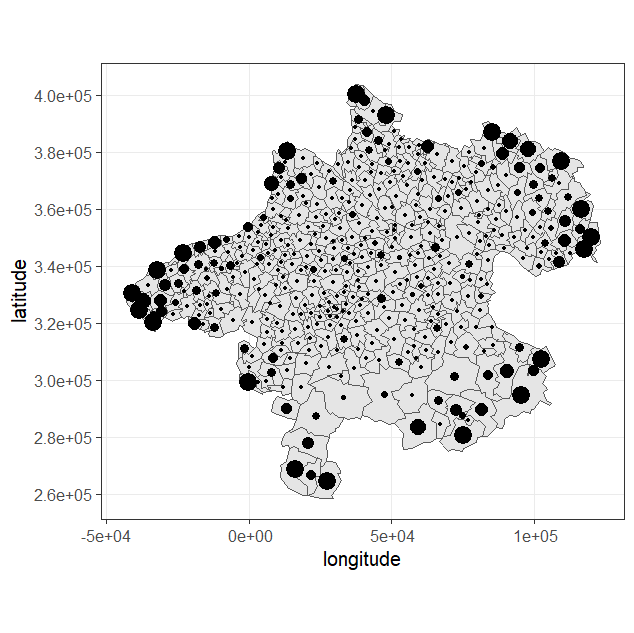
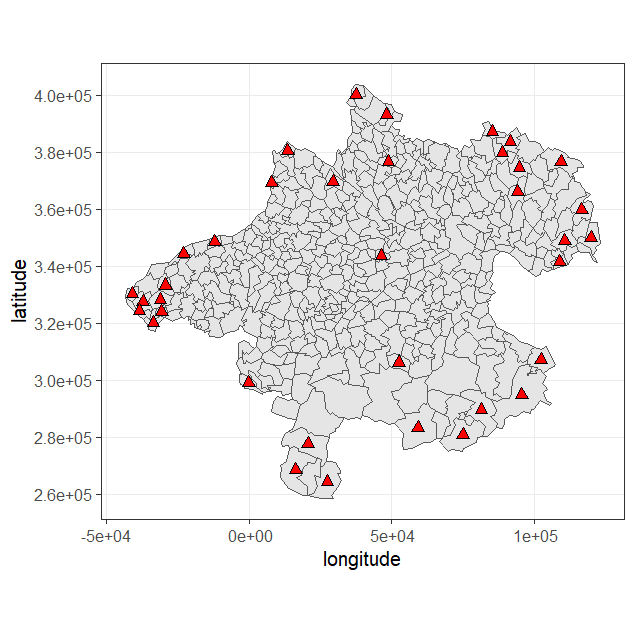
Figure 4: Our measure (left panel) and exact 36-point design found by taking the optimal design from 100 random draws from the virtual noise measure (right panel) for Example 3 .

The D-efficiencies for different methods used to construct the optimal 36-point exact design are given in Table 8. As in the other examples, these efficiencies are reported with respect to our bound. The appendix contains those for additional values of $n$ from $n=4$ to $n=40$.

Table 4: D-efficiencies for Example 3

	D-eff
R-VN (highest efficiency)	0.9915
R-VN (median efficiency)	0.9702
R-UNIF (highest efficiency)	0.8405
R-UNIF (median efficiency)	0.6689
BKSF	0.9965

Discussion

The present paper complements and in a certain sense completes the research in Müller and Pázman (2003). The virtual noise approach now exhibits the convexity property it previously lacked. The formulated equivalence theorem allows for calculating a general upper bound for designs in Gaussian process regression, a key methodology in many application fields. This upper bound for the first time offers the possibility to calibrate and scale other design methods proposed in the literature.

Furthermore, our “importance measures” can be used to directly produce exact designs, be it by taking quantiles or by randomly sampling from them. However, typically for all the examples considered, also those not reported here, the adaptation of Brimkulov et al. (1980) using the approximate sensitivity function from Fedorov (1996) performed slightly better than taking the quantiles from the measure given by the virtual noise representation, which in turn was better than the method suggested by Dette et al. (2016). Therefore, for practical purposes a combined approach using the approximate sensitivity function for finding designs and the upper bound derived from the virtual noise representation for evaluating them seems to be the most suitable avenue. Even when one prefers not to use an optimal design, but a classical one such as fractional factorial, orthogonal array, latin hypercube, etc. our bound can be used to judge how much efficiency would be sacrificed.

Appendix

Appendix A.1 Proof of Theorem 1 on concavity

For any $u\in\mathbb{R}^{N}$ define the function

$$\xi\in\Xi\to\gamma_{u}(\xi)=\left\{\begin{array}[]{ll}u^{\mathrm{\scriptscriptstyle T}}\left\{C+W(\xi)\right\}^{-1}u&\text{if }\text{supp}(\xi)=\mathcal{X}\\ u^{\prime\mathrm{\scriptscriptstyle T}}\left\{C^{\prime}+W^{\prime}(\xi)\right\}^{-1}u^{\prime}&\,\text{if }\text{supp}(\xi)\neq\mathcal{X}\\ \end{array}\right.,$$

where $C^{\prime}$, $W^{\prime}(\xi)$, $u^{\prime}$ are submatrices of $C$, $W(\xi)$, $u$, respectively with rows and/or columns corresponding to the points of $\text{supp}(\xi)$.

Lemma A1

The function $\xi\in\Xi\to\gamma_{u}(\xi)$ is concave.

Proof. We start by proving the concavity on $\Xi_{+}=\left\{\xi\in\Xi:\text{supp}(\xi)=\mathcal{X}\right\}$. Consider an auxiliary function

$$\psi_{u}(\alpha):\alpha\in(0,1)\rightarrow\gamma_{u}(\xi_{\alpha}),$$

with $\xi_{\alpha}(x)=(1-\alpha)\xi(x)+\alpha\mu(x);\quad\xi,\mu\in\Xi_{+},\alpha\in(0,1)$. The concavity of $\gamma_{u}(\xi)$ on $\Xi_{+}$ will be proven if we show that

$$\frac{d^{2}\psi_{u}(\alpha)}{d\alpha^{2}}\leq 0$$

for any $\xi,\mu\in\Xi_{+}$ and any $\alpha\in\left(0,1\right)$.

We can write

$$\psi_{u}(\alpha)=u^{\mathrm{\scriptscriptstyle T}}\left\{H(\xi_{\alpha})\right\}^{-1}u,$$

with

$$H(\xi_{\alpha})=\left[\left(C-\kappa I\right)+\frac{\kappa}{n}\,\text{diag}\left\{\frac{1}{\xi_{\alpha}(\cdot)}\right\}\right].$$

Notice that the matrix $\left(C-\kappa I\right)$ is positive definite, hence also $H(\xi_{\alpha})$ is positive definite.

From the rule for the derivative of an inverse matrix we obtain

$$\frac{d\psi_{u}(\alpha)}{d\alpha} = -\frac{\kappa}{n}\,u^{\mathrm{\scriptscriptstyle T}}H^{-1}(\xi_{\alpha})\left\{\frac{d}{d\alpha}\,\text{diag}\left(\frac{1}{\xi_{\alpha}(\cdot)}\right)\right\}\,H^{-1}(\xi_{\alpha})u$$

$$= \frac{\kappa}{n}\,u^{\mathrm{\scriptscriptstyle T}}H^{-1}(\xi_{\alpha})\,\text{diag}\left\{\frac{1}{\xi_{\alpha}^{2}(\cdot)}\right\}\text{diag}\left\{\mu(\cdot)-\xi(\cdot)\right\}\,H^{-1}(\xi_{\alpha})u$$

$$= \frac{\kappa}{n}\,u^{\mathrm{\scriptscriptstyle T}}T^{\mathrm{\scriptscriptstyle T}}(\xi_{\alpha})\,\text{diag}\left\{\mu(\cdot)-\xi(\cdot)\right\}\,T(\xi_{\alpha})u,$$

where

$$T(\xi_{\alpha})=\left[\left(C-\kappa I\right)\text{diag}\left\{\xi_{\alpha}(\cdot)\right\}+\frac{\kappa}{n}I\right]^{-1}.$$

Hence

$$\frac{d^{2}\psi_{u}(\alpha)}{d\alpha^{2}}$$

$$= -\frac{\kappa}{n}\,u^{\mathrm{\scriptscriptstyle T}}T^{\mathrm{\scriptscriptstyle T}}(\xi_{\alpha})\,\text{diag}\{\mu(\cdot)-\xi(\cdot)\}\,\left(C-\kappa I\right)T^{\mathrm{\scriptscriptstyle T}}(\xi_{\alpha})$$

$$\times\,\text{diag}\{\mu(\cdot)-\xi(\cdot)\}\,T(\xi_{\alpha})u$$

$$-\frac{\kappa}{n}\,u^{\mathrm{\scriptscriptstyle T}}T^{\mathrm{\scriptscriptstyle T}}(\xi_{\alpha})\,\text{diag}\{\mu(\cdot)-\xi(\cdot)\}$$

$$\times T(\xi_{\alpha})\left(C-\kappa I\right)\text{diag}\{\mu(\cdot)-\xi(\cdot)\}\,T(\xi_{\alpha})u,$$

which is nonpositive since the matrix

$$\left(C-\kappa I\right)T^{\mathrm{\scriptscriptstyle T}}(\xi_{\alpha}) = \left(C-\kappa I\right)\left[\text{diag}\left\{\xi_{\alpha}(\cdot)\right\}\left(C-\kappa I\right)+\frac{\kappa}{n}I\right]^{-1}$$

$$= \left[\text{diag}\left\{\xi_{\alpha}(\cdot)\right\}+\frac{\kappa}{n}\left(C-\kappa I\right)^{-1}\right]^{-1}$$

is symmetric positive definite.

To finish the proof take arbitrary $\xi,\mu\in\Xi$ and sequences $\{\xi_{k}\},\{\mu_{k}\}$ of elements of $\Xi_{+}$ converging to $\xi$ and $\mu$. From the inequality

$$\gamma_{u}\{(1-\alpha)\xi_{k}+\alpha\mu_{k}\}\geq(1-\alpha)\gamma_{u}(\xi_{k})+\alpha\gamma_{u}(\mu_{k}),$$

valid for each $k$, we obtain by the continuity of $\xi\in\Xi\to\gamma_{u}(\xi)$, see Lemma A2, that the same inequality also holds for $\xi$ and $\mu$. ∎

Proof of Theorem 1

Since for any $t\in\mathbb{R}^{p}.$ we have

$$t^{\mathrm{\scriptscriptstyle T}}M(\xi)t=\gamma_{Ft}(\xi),$$

we can write for any $\xi,\mu\in\Xi$

$$t^{\mathrm{\scriptscriptstyle T}}M\{(1-\alpha)\xi+\alpha\mu\}t\geq(1-\alpha)t^{\mathrm{\scriptscriptstyle T}}M(\xi)t+\alpha t^{\mathrm{\scriptscriptstyle T}}M(\mu)t,$$

which means that

$$M\{(1-\alpha)\xi+\alpha\mu\}\geq(1-\alpha)M(\xi)+\alpha M(\mu)$$

in the Löwner ordering. From the monotonicity of $\Phi$ we have

$$\Phi\left[M\{(1-\alpha)\xi+\alpha\mu\}\right]\geq\Phi\left\{(1-\alpha)M(\xi)+\alpha M(\mu)\right\}$$

and from the concavity of $\Phi\,$ we have

$$\Phi\left\{(1-\alpha)M(\xi)+\alpha M(\mu)\right\}\geq(1-\alpha)\Phi\{M(\xi)\}+\alpha\Phi\{M(\mu)\}.$$

∎

Appendix A.2 Proof of the equivalence theorem (Theorem 2)

Since the function

$$\xi\in\Xi\rightarrow\Phi\{M(\xi)\}$$

is concave, the design $\bar{\xi}$ is $\Phi-$optimal if and only if for every $\mu\in\Xi$ we have, see Lemma A3,

$$\pi\left(\bar{\xi},\mu\right)=\lim_{\alpha\rightarrow 0^{+}}\frac{\Phi\left\{M\left(\xi_{\alpha}^{\mu}\right)\right\}-\Phi\left\{M\left(\bar{\xi}\right)\right\}}{\alpha}\>\leq\>0,$$

where we used the notation

$$\xi_{\alpha}^{\mu}(x)=(1-\alpha)\bar{\xi}(x)+\alpha\mu(x).$$

We have

$$\lim_{\alpha\rightarrow 0^{+}}\frac{\Phi\left\{M\left(\xi_{\alpha}^{\mu}\right)\right\}-\Phi\left\{M\left(\bar{\xi}\right)\right\}}{\alpha} = \sum_{i,j=1}^{p}\lim_{\alpha\rightarrow 0^{+}}\frac{\Phi\left\{M\left(\xi_{\alpha}^{\mu}\right)\right\}-\Phi\left\{M\left(\bar{\xi}\right)\right\}}{M_{ij}\left(\xi_{\alpha}^{\mu}\right)-M_{ij}\left(\bar{\xi}\right)}\times$$

$$\phantom{\sum_{i,j=1}^{p}}\times\lim_{\alpha\rightarrow 0^{+}}\frac{M_{ij}\left(\xi_{\alpha}^{\mu}\right)-M_{ij}\left(\bar{\xi}\right)}{\alpha}$$

$$= \sum_{i,j=1}^{p}\lim_{\xi\rightarrow\bar{\xi}}\,\frac{\Phi\left\{M\left(\xi\right)\right\}-\Phi\left\{M\left(\bar{\xi}\right)\right\}}{M_{ij}\left(\xi\right)-M_{ij}\left(\bar{\xi}\right)}\times$$

$$\phantom{\sum_{i,j=1}^{p}}\times\lim_{\alpha\rightarrow 0^{+}}\frac{M_{ij}\left(\xi_{\alpha}^{\mu}\right)-M_{ij}\left(\bar{\xi}\right)}{\alpha},$$

since $\underset{\alpha\rightarrow 0^{+}}{\lim}\,\xi_{\alpha}^{\mu}=\bar{\xi}$. Therefore, we obtain

$$\lim_{\alpha\rightarrow 0^{+}}\frac{\Phi\left\{M\left(\xi_{\alpha}^{\mu}\right)\right\}-\Phi\left\{M\left(\bar{\xi}\right)\right\}}{\alpha} = \text{tr}\left[\nabla\Phi\left(M\right)\bigl{|}_{M=M\left(\bar{\xi}\right)}\>\lim_{\alpha\rightarrow 0^{+}}\frac{M\left(\xi_{\alpha}^{\mu}\right)-M\left(\bar{\xi}\right)}{\alpha}\right]$$

$$= \text{tr}\left[\nabla\Phi\left(M\right)\bigl{|}_{M=M\left(\bar{\xi}\right)}\>\frac{\kappa}{n}F^{\mathrm{\scriptscriptstyle T}}T^{\mathrm{\scriptscriptstyle T}}\left(\bar{\xi}\right)\text{diag}\left(\mu-\bar{\xi}\right)T\left(\bar{\xi}\right)F\right]$$

$$= \frac{\kappa}{n}\sum_{x\in\mathcal{X}}\left\{\mu(x)-\bar{\xi}(x)\right\}h(x,\bar{\xi}),$$

as follows from (19) and (20) in Lemma A4 and from the definition of $h(x,\bar{\xi})$ at the beginning of Section 2.5, just before Theorem 2. Hence we finally obtain

$$\pi\left(\bar{\xi},\mu\right)=\frac{\kappa}{n}\sum_{x\in\mathcal{X}}\left\{\mu(x)-\bar{\xi}(x)\right\}h(x,\bar{\xi}).$$ (10)

Therefore, $\bar{\xi}\in\Xi$ is $\Phi-$optimal if and only if for every $\mu\in\Xi$ we have

$$\sum_{x\in\mathcal{X}}\mu(x)h(x,\bar{\xi})\leq\sum_{x\in\mathcal{X}}\bar{\xi}(x)h(x,\bar{\xi}).$$ (11)

Since this expression is linear in $\mu$ and since the convex hull of the set of all exact $n$-point designs is the convex set $\Xi$, we do not need to consider all designs $\mu$ from $\Xi,$ but just the exact $n$-point designs. Hence the validity of the inequality (7) in Theorem 2 for all such $n$-point measures is equivalent to the validity of (11) for all $\mu\in\Xi$.

From (10) it follows that the inequalities (8) in Theorem 2 imply that for every $\mu\in\Xi$ we have

$$\pi\left(\bar{\xi},\mu\right)\leq\delta.$$

According to Lemma A3 it follows that the inequality (9) holds as well. ∎

Appendix A.3 Adaptation of the algorithm from Fedorov (1996) for A-optimality

Sensitivity function for the D-criterion

Consider the linear regression model with i.i.d. errors,

$$y(x)=f(x)^{\mathrm{\scriptscriptstyle T}}\theta+\varepsilon(x),$$

where $E\{\varepsilon(x)\}=0$, $\text{var}\,\{\varepsilon(x)\}=\sigma^{2}_{\varepsilon}$, and $E\{\varepsilon(x)\varepsilon(x^{\prime})\}=0$ $\forall x,x^{\prime}\in\mathcal{X}$.

The information matrix for a design $\xi\in\Xi$ is

$$M_{\xi}=\frac{1}{\sigma^{2}_{\varepsilon}}\sum_{x\in\mathcal{X}}\xi(x)f(x)f(x)^{\mathrm{\scriptscriptstyle T}}.$$

We also consider a one-point design at $\bar{x}\in\mathcal{X}$ denoted by $\xi_{\bar{x}}$. Its information matrix is

$$M_{\xi_{\bar{x}}}=\frac{1}{\sigma^{2}_{\varepsilon}}f(\bar{x})f(\bar{x})^{\mathrm{\scriptscriptstyle T}}.$$

Let the information matrix of the convex combination $\xi_{\bar{x}}^{\alpha}=(1-\alpha)\xi+\alpha\xi_{\bar{x}}$ of those two designs be denoted by

$$M_{\alpha}=(1-\alpha)M_{\xi}+\alpha M_{\xi_{\bar{x}}}.$$

For some concave criterion function $\Phi(M)$, the directional derivative of $\Phi(\cdot)$ at the design $\xi$ in the direction of $\xi_{\bar{x}}$, the so-called sensitivity function, is

$$\phi(\bar{x};\xi) = \lim_{\alpha\rightarrow 0^{+}}\frac{\Phi(M_{\alpha})-\Phi(M_{\xi})}{\alpha}$$ (12)

$$= \lim_{\alpha\rightarrow 0^{+}}\text{tr}\left\{\nabla_{M}\Phi(M_{\alpha})\,\frac{\partial M_{\alpha}}{\partial\alpha}\right\}$$

$$= \lim_{\alpha\rightarrow 0^{+}}\text{tr}\left\{\nabla_{M}\Phi(M_{\alpha})\left(M_{\xi_{\bar{x}}}-M_{\xi}\right)\right\}$$

$$= \text{tr}\left\{\nabla_{M}\Phi(M_{\xi})\left(M_{\xi_{\bar{x}}}-M_{\xi}\right)\right\}$$

$$= \frac{1}{\sigma^{2}_{\varepsilon}}f(\bar{x})^{\mathrm{\scriptscriptstyle T}}\nabla_{M}\Phi(M_{\xi})f(\bar{x})-\text{tr}\left\{\nabla_{M}\Phi(M_{\xi})\,M_{\xi}\right\}.$$

In the case of D-optimality, we prefer here the criterion function $\Phi_{D}(M)=\log\det(M)$, so $\nabla_{M}\Phi_{D}(M)=M^{-1}$. Plugging this into (12) yields

$$\phi_{D}(\bar{x};\xi) = \frac{1}{\sigma^{2}_{\varepsilon}}f(\bar{x})^{\mathrm{\scriptscriptstyle T}}M_{\xi}^{-1}f(\bar{x})-\text{tr}\left(M_{\xi}^{-1}M_{\xi}\right)$$ (13)

$$= \frac{1}{\sigma^{2}_{\varepsilon}}f(\bar{x})^{\mathrm{\scriptscriptstyle T}}M_{\xi}^{-1}f(\bar{x})-\mathrm{dim}(\theta).$$

Up to a constant, expression (13) is equal to

$$\frac{E\left[\left\{y(\bar{x})-\hat{y}(\bar{x})\right\}^{2}\right]}{\sigma^{2}_{\varepsilon}}=\frac{\sigma^{2}_{\varepsilon}+f(\bar{x})^{\mathrm{\scriptscriptstyle T}}M_{\xi}^{-1}f(\bar{x})}{\sigma^{2}_{\varepsilon}}=1+\frac{f(\bar{x})^{\mathrm{\scriptscriptstyle T}}M_{\xi}^{-1}f(\bar{x})}{\sigma^{2}_{\varepsilon}}.$$ (14)

In the correlated case with no replications, Fedorov (1996) suggests to replace the numerator in (14) by the unconditional and the denominator in (14) by the conditional variance. Let $\mathcal{T}=\{x_{1},\ldots,x_{n}\}\subset\mathcal{X}$ denote an exact n-point design, let $C(\mathcal{T})$ be the $n\times n$ submatrix of the covariance matrix $C$ for the set of points in $\mathcal{T}$, and let $F(\mathcal{T})$ be the $n\times p$ design matrix with elements $F_{i,j}(\mathcal{T})=f_{j}(x_{i})$. Let $k(x,x^{\prime})=\text{cov}\,\{\varepsilon(x),\varepsilon(x^{\prime})\}$ and for a point $\bar{x}\in\mathcal{X}\backslash\mathcal{T}$, let $k(\bar{x},\mathcal{T})=\left(k(\bar{x},x_{1}),\ldots,k(\bar{x},x_{n})\right)^{\mathrm{\scriptscriptstyle T}}$. In the correlated case, Fedorov (1996) therefore replaces expression (14) with

$$\frac{E\left[\left\{y(\bar{x})-\hat{y}(\bar{x})\right\}^{2}\right]}{\tilde{\sigma}^{2}(\bar{x})}=\frac{\tilde{\sigma}^{2}(\bar{x})+\tilde{f}(\bar{x})^{\mathrm{\scriptscriptstyle T}}M_{\mathcal{T}}^{-1}\tilde{f}(\bar{x})}{\tilde{\sigma}^{2}(\bar{x})},$$

where

$$\tilde{\sigma}^{2}(\bar{x})=k(\bar{x},\bar{x})-k(\bar{x},\mathcal{T})^{\mathrm{\scriptscriptstyle T}}C^{-1}(\mathcal{T})k(\bar{x},\mathcal{T}),$$

is the conditional variance, $\tilde{f}(\bar{x})$ is

$$\tilde{f}(\bar{x})=f(\bar{x})-F(\mathcal{T})^{\mathrm{\scriptscriptstyle T}}C^{-1}(\mathcal{T})k(\bar{x},\mathcal{T}),$$

and the information matrix is

$$M_{\mathcal{T}}=F(\mathcal{T})^{\mathrm{\scriptscriptstyle T}}C^{-1}(\mathcal{T})F(\mathcal{T}).$$

It can be shown that for D-optimality this approximate sensitivity function is equal to the factor by which the determinant of the information matrix is increased by adding design point $\bar{x}$.

Sensitivity function for the A-criterion

In the case of A-optimality, we use the criterion $\Phi_{A}(M)=-\mathrm{tr}\left(M^{-1}\right)$. We therefore have $\nabla_{M}\Phi_{A}(M)=-\left(-M^{-2}\right)^{\mathrm{\scriptscriptstyle T}}=M^{-2}$ and the directional derivative is

$$\phi_{A}(\bar{x};\xi)=\frac{1}{\sigma^{2}_{\varepsilon}}f(\bar{x})^{\mathrm{\scriptscriptstyle T}}M_{\xi}^{-2}f(\bar{x})-\mathrm{tr}\left(M_{\xi}^{-1}\right).$$

In accordance with the case of D-optimality outlined above, we obtain the approximate sensitivity function by analogous replacements. Therefore, the sensitivity function we eventually use in some of our examples is

$$\tilde{\phi}_{A}(\bar{x};\mathcal{T})=\frac{1}{\tilde{\sigma}^{2}(\bar{x})}\tilde{f}(\bar{x})^{\mathrm{\scriptscriptstyle T}}M_{\mathcal{T}}^{-2}\tilde{f}(\bar{x})-\mathrm{tr}\left(M_{\mathcal{T}}^{-1}\right).$$

Appendix A.4 Outline of algorithm from Fedorov (1996)

Algorithm 1 contains the description of our implementation for a finite design grid of the algorithm proposed in Fedorov (1996).

Input: Design grid $\mathcal{X}$ of possible design points; design size $n$; initial design $\mathcal{T}_{0}$; (approximate) sensitivity function $\tilde{\phi}(x;\mathcal{T}).$

Output: Exact design $\mathcal{T}$ found by algorithm.

1

2abort = false ;

3 $\mathcal{T}=\mathcal{T}_{0}$;

4 while not abort do

5       for $i=1$ to $n$ do

6             Let $x_{i}$ be the $i$^th design point in $\mathcal{T}$;

7             $\mathcal{T}_{-i}=\mathcal{T}\backslash\{x_{i}\}$;

8             $\mathtt{s[i]}=\tilde{\phi}(x_{i};\mathcal{T}_{-i})$;

9            

10       end for

11      $\mathtt{sens\_drop}=\min(\mathtt{s})$;

12       Let $\mathtt{k}$ be the index where $\mathtt{s[k]}=\mathtt{sens\_drop}$;

13       Let $\mathcal{C}=\mathcal{X}\backslash\mathcal{T}_{-k}$;

14       $m=\text{card}(\mathcal{C})$;

15       for $i=1$ to $m$ do

16             Let $\bar{x}_{i}$ be the $i$^th design point in the candidate set $\mathcal{C}$;

17             $\mathtt{t[i]}=\tilde{\phi}(\bar{x}_{i};\mathcal{T}_{-k})$;

18            

19       end for

20      $\mathtt{sens\_add}=\max(\mathtt{t})$;

21       Let $\mathtt{l}$ be the index where $\mathtt{t[l]}=\mathtt{sens\_add}$;

22       $\mathcal{T}=\mathcal{T}_{-k}\cup\bar{x}_{l}$;

23       if $\mathtt{sens\_add}-\mathtt{sens\_drop}\leq 0$ then

24             abort = true ;

25            

26       end if

27      

28 end while

Algorithm 1 Algorithm proposed by Fedorov (1996) for a finite design grid

Appendix A.5 Miscellanea

Lemma A2: the continuity lemma

The function $\gamma_{u}(\xi)$ defined in Lemma A1 is continuous on $\Xi$ and $M(\xi)$ is continuous on $\Xi$ as well.

Proof. Take $\xi_{k}\in\Xi$ such that $\lim_{k\to\infty}\xi_{k}=\xi$. The equality $\lim_{k\to\infty}\gamma_{u}(\xi_{k})=\gamma_{u}(\xi)$ is evident if $\text{supp}(\xi)=\mathcal{X}$, or more generally if $\bigcup_{k_{0}=1}^{\infty}\bigcap_{k\geq k_{0}}\text{supp}(\xi_{k})=\text{supp}(\xi)$. To clarify how to do the proof in the opposite case we suppose that $\text{supp}(\xi)=\mathcal{X}$, but $\bigcup_{k_{0}=1}^{\infty}\bigcap_{k\geq k_{0}}\text{supp}(\xi_{k})$ has one point less than the set $\text{supp}(\xi)$, say the point $x_{1}$. By a basic property of inverse matrices we have

$$\left[\left\{C+W(\xi_{k})\right\}^{-1}\right]_{ij}=\frac{(-1)^{i+j}\det\left\{C+W(\xi_{k})\right\}^{i,j}}{\det\left\{C+W(\xi_{k})\right\}},$$ (15)

where $\left\{C+W(\xi_{k})\right\}^{i,j}$ is the submatrix of $\left\{C+W(\xi_{k})\right\}$ after omitting the $i$-th row and $j$-th column. For $k\to\infty$ (15) tends to zero for $i=1$ or $j=1$, but to a nonzero number when $i\neq 1$ and $j\neq 1$. This can be seen when using the definition of a determinant as a sum of products of the elements of the matrix. When $k\to\infty$, some terms of these sums in the numerator and the denominator converge to $\infty$ much slower than the others, so we can neglect them. We proceed similarly when $\bigcup_{k_{0}=1}^{\infty}\bigcap_{k\geq k_{0}}\text{supp}(\xi_{k})\cup\{x_{1},x_{2}\}=\text{supp}(\xi)$, etc.. ∎

For the reader’s convenience we prove a statement from convex theory, see e.g. Rockafellar (1970).

Lemma A3

If a function $\phi:\xi\in\Xi\rightarrow\phi(\xi)\in\mathbb{R}$ is concave, then for any $\bar{\xi},\mu\in\Xi$ the function

$$\alpha\in\left(0,1\right)\rightarrow\frac{\phi\left\{(1-\alpha)\bar{\xi}+\alpha\mu\right\}-\phi\!\left(\bar{\xi}\right)}{\alpha}$$

is nonincreasing. Hence for any $\bar{\xi}\in\Xi$ and any $\mu\in\Xi$ there exists the limit

$$\lim_{\alpha\rightarrow 0^{+}}\frac{\phi\left\{(1-\alpha)\bar{\xi}+\alpha\mu\right\}-\phi\!\left(\bar{\xi}\right)}{\alpha}\equiv\pi\left(\bar{\xi},\mu\right),$$

and we have

$$\bar{\xi}\in\arg\max_{\xi\in\Xi}\phi(\xi)$$

if and only if

$$\forall\>\mu\in\Xi\,\,\,\,\,\,\,\,\,\pi\left(\bar{\xi},\mu\right)\>\leq\>0.\quad\quad$$ (16)

If for some $\delta>0$ and for every $\mu\in\Xi$ we have

$$\pi\left(\bar{\xi},\mu\right)\leq\delta,$$

then $\displaystyle\phi\left(\bar{\xi}\right)\geq\underset{\xi\in\Xi}{\max}\ \phi(\xi)-\delta$.

Proof

Take $\,0<\alpha_{1}<\alpha_{2}<1$. From the concavity of $\phi(\xi)$ we obtain

$$\phi\left\{(1-\alpha_{1})\bar{\xi}+\alpha_{1}\mu\right\}-\phi\!\left(\bar{\xi}\right)$$

$$= \phi\left[\frac{\alpha_{1}}{\alpha_{2}}\left\{(1-\alpha_{2})\bar{\xi}+\alpha_{2}\mu\right\}+\left(1-\frac{\alpha_{1}}{\alpha_{2}}\right)\bar{\xi}\right]-\phi\!\left(\bar{\xi}\right)$$

$$\geq \frac{\alpha_{1}}{\alpha_{2}}\,\phi\left\{(1-\alpha_{2})\bar{\xi}+\alpha_{2}\mu\right\}+\left(1-\frac{\alpha_{1}}{\alpha_{2}}\right)\phi\!\left(\bar{\xi}\right)-\phi\!\left(\bar{\xi}\right)$$

$$= \frac{\alpha_{1}}{\alpha_{2}}\left[\phi\left\{(1-\alpha_{2})\bar{\xi}+\alpha_{2}\mu\right\}-\phi\!\left(\bar{\xi}\right)\right].$$

We multiply this inequality by $1/\alpha_{1}$ to prove the first statement of the Lemma.

If $\bar{\xi}\in\underset{\xi\in\Xi}{\arg\max}\ \phi(\xi),$ then for any $\mu$ and $\alpha$ we evidently have

$$\frac{\phi\left\{(1-\alpha)\bar{\xi}+\alpha\mu\right\}-\phi\!\left(\bar{\xi}\right)}{\alpha}\leq 0$$

and this inequality does also hold for $\alpha\rightarrow 0^{+}.$

On the other hand, suppose that there is $\mu\in\Xi$ such that $\phi(\mu)>\phi\!\left(\bar{\xi}\right)$. Then for every $\alpha\in\left(0,1\right)$ we have

$$\frac{\phi\left\{(1-\alpha)\bar{\xi}+\alpha\mu\right\}-\phi\!\left(\bar{\xi}\right)}{\alpha}$$

$$\geq \frac{(1-\alpha)\phi\!\left(\bar{\xi}\right)+\alpha\phi\!\left(\mu\right)-\phi\!\left(\bar{\xi}\right)}{\alpha}$$

$$= \phi\!\left(\mu\right)-\phi\!\left(\bar{\xi}\right)>0,$$

and by taking the limit for $\alpha\rightarrow 0$ we see that (16) does not hold.

If

$$\forall_{\mu\in\mathcal{X}}\>\pi\left(\bar{\xi},\mu\right)\leq\delta,$$

then from the concavity of $\phi(\xi)$ we obtain for every $\mu\in\Xi$

$$\phi(\mu)-\phi(\bar{\xi}) = \frac{(1-\alpha)\phi(\bar{\xi})+\alpha\phi(\mu)-\phi(\bar{\xi})}{\alpha}$$

$$\leq \frac{\phi\{(1-\alpha)\bar{\xi}+\alpha\mu\}-\phi(\bar{\xi})}{\alpha}\leq\pi\left(\bar{\xi},\mu\right)\leq\delta.$$

Hence $\displaystyle\phi\left(\bar{\xi}\right)\geq\underset{\mu\in\Xi}{\max}\ \phi(\mu)-\delta$. ∎

Lemma A4

The matrix

$$L\left(\xi\right)\equiv F^{\mathrm{\scriptscriptstyle T}}\left[\text{diag}\left\{\xi\left(\cdot\right)\right\}\left(C-\kappa I\right)+\frac{\kappa}{n}I\right]^{-1}\text{diag}\left\{\xi\left(\cdot\right)\right\}F$$ (17)

is well defined and continuous on $\Xi$.

For every $\xi\in\Xi$ we have $L\left(\xi\right)=M\left(\xi\right)$ with $M\left(\xi\right)$ defined in (3) and (4).

For every $\bar{\xi}\in\Xi$ and $\mu\in\Xi$ the right-hand limit

$$\lim_{\alpha\rightarrow 0^{+}}\frac{L\left\{\left(1-\alpha\right)\bar{\xi}+\alpha\mu\right\}-L\left(\bar{\xi}\right)}{\alpha}$$

is well defined and it is a continuous function of $\bar{\xi}$ on the whole set $\Xi$. On the set $\Xi_{+}$ it is equal to the derivative $\frac{\partial L\left(\xi_{\alpha}^{\mu}\right)}{\partial\alpha}\bigl{|}_{\alpha=0}=\frac{\partial M\left(\xi_{\alpha}^{\mu}\right)}{\partial\alpha}\bigl{|}_{\alpha=0}$.

Proof

We denote $Z\left(\xi\right)=\left[\text{diag}\left\{\xi\left(\cdot\right)\right\}\left(C-\kappa I\right)+\frac{\kappa}{n}I\right]$. To see the correctness of the definition and the continuity of $L\left(\xi\right)$, we must prove the existence of the matrix $Z\left(\xi\right)^{-1}$ used in (17). Without loss of generality we can suppose that $\xi\left(x_{i}\right)>0$ for $i=1,\ldots,k$ and $\xi\left(x_{i}\right)=0$ for $i=k+1,...,N$, where $k\leq N$. Let us write $Z\left(\xi\right)=\left(\begin{array}[]{cc}V&R\\ P&T\end{array}\right)$, where $V$ is a $k\times k$ matrix and $T$ is a $\left(N-k\right)\times\left(N-k\right)$ matrix. Evidently $P=0.$ According to Harville (1997), Lemma 8.5.4, if the inverse matrices $V^{-1}$ and $T^{-1}$ exist, then the inverse of the partitioned matrix exists as well, and

$$\left(\begin{array}[]{cc}V&R\\ 0&T\end{array}\right)^{-1}=\left(\begin{array}[]{cc}V^{-1}&-V^{-1}RT^{-1}\\ 0&T^{-1}\end{array}\right).$$

We can write

$$\text{diag}\left\{\xi\left(\cdot\right)\right\}=\left(\begin{array}[]{cc}\text{diag}^{\prime}\left\{\xi\left(\cdot\right)\right\}&0\\ 0&0\end{array}\right),$$

where the $k\times k$ matrix $\text{diag}^{\prime}\left\{\xi\left(\cdot\right)\right\}$ has the $k$ positive elements of $\xi$ on its diagonal. Consequently

$$V = \text{diag}^{\prime}\left\{\xi\left(\cdot\right)\right\}\left(C^{\prime}-\kappa I^{\prime}\right)+\frac{\kappa}{n}I^{\prime}$$

$$= \text{diag}^{\prime}\left\{\xi\left(\cdot\right)\right\}\left[\left(C^{\prime}-\kappa I^{\prime}\right)+\frac{\kappa}{n}\text{diag}^{\prime}\left\{\xi^{-1}\left(\cdot\right)\right\}\right],$$

where the prime denotes the $k\times k$ submatrix of the corresponding matrix. The symmetric matrix

$$\left[\left(C^{\prime}-\kappa I^{\prime}\right)+\frac{\kappa}{n}\text{diag}^{\prime}\left\{\xi^{-1}\left(\cdot\right)\right\}\right]$$

is positive definite, hence its inverse exists and $V^{-1}$ exists as well. Finally $T=\frac{\kappa}{n}I^{*}$, where the star denotes the $\left(N-k\right)\times\left(N-k\right)$ submatrix, so $T^{-1}=\frac{n}{\kappa}I^{*}.$

The continuity of $L\left(\xi\right)$ on $\Xi$ is now evident from (17).

To prove $L\left(\xi\right)=M\left(\xi\right)$, let us denote the upper $k\times p$ and lower $\left(N-k\right)\times p$ submatrices of $F$ by $F^{\prime}$ and $F^{*}$, respectively. We have

$$L\left(\xi\right) = \left(\begin{array}[]{c}F^{\prime}\\ F^{*}\end{array}\right)^{\mathrm{\scriptscriptstyle T}}\left(\begin{array}[]{cc}V^{-1}&-V^{-1}RT^{-1}\\ 0&T^{-1}\end{array}\right)\left(\begin{array}[]{c}\text{diag}^{\prime}\left\{\xi\left(\cdot\right)\right\}F^{\prime}\\ 0\end{array}\right)$$

$$= \left(F^{\prime}\right)^{\mathrm{\scriptscriptstyle T}}V^{-1}\text{diag}^{\prime}\left\{\xi\left(\cdot\right)\right\}F^{\prime}$$

$$= \left(F^{\prime}\right)^{\mathrm{\scriptscriptstyle T}}\left[\left(C^{\prime}-\kappa I^{\prime}\right)+\frac{\kappa}{n}\text{diag}^{\prime}\left\{\xi^{-1}\left(\cdot\right)\right\}\right]^{-1}F^{\prime}=M\left(\xi\right),$$

as follows from Eq. (4).

Let us suppose first that $\bar{\xi}\in\Xi_{+}$. Using the standard rules for the derivatives of matrices, we obtain from (17)

$$\frac{\partial L\left(\xi_{\alpha}^{\mu}\right)}{\partial\alpha}\biggl{|}_{\alpha=0} = -\,F^{\mathrm{\scriptscriptstyle T}}Z^{-1}\left(\bar{\xi}\right)\,\text{diag}\left(\mu-\bar{\xi}\right)\left(C-\kappa I\right)Z^{-1}\left(\bar{\xi}\right)\text{diag}\left(\bar{\xi}\right)F$$ (19)

$$+\,F^{\mathrm{\scriptscriptstyle T}}Z^{-1}\left(\bar{\xi}\right)\text{diag}\left(\mu-\bar{\xi}\right)F$$

$$= F^{\mathrm{\scriptscriptstyle T}}Z^{-1}\left(\bar{\xi}\right)\text{diag}\left(\mu-\bar{\xi}\right)\left[I-\left(C-\kappa I\right)Z^{-1}\left(\bar{\xi}\right)\text{diag}\left(\bar{\xi}\right)\right]F$$

$$= F^{\mathrm{\scriptscriptstyle T}}Z^{-1}\left(\bar{\xi}\right)\text{diag}\left(\mu-\bar{\xi}\right)\frac{\kappa}{n}\left\{Z^{\mathrm{\scriptscriptstyle T}}\left(\bar{\xi}\right)\right\}^{-1}F$$

$$= \frac{\kappa}{n}F^{\mathrm{\scriptscriptstyle T}}T^{\mathrm{\scriptscriptstyle T}}\left(\bar{\xi}\right)\text{diag}\left(\mu-\bar{\xi}\right)T\left(\bar{\xi}\right)F,$$

which is well defined and continuous on $\Xi_{+}$. The equality

$$\frac{\kappa}{n}\left\{Z^{\mathrm{\scriptscriptstyle T}}\left(\bar{\xi}\right)\right\}^{-1}=I-\left(C-\kappa I\right)Z^{-1}\left(\bar{\xi}\right)\text{diag}\left(\bar{\xi}\right)$$

for $Z^{\mathrm{\scriptscriptstyle T}}\left(\bar{\xi}\right)=\left(C-\kappa I\right)\text{diag}\left(\bar{\xi}\right)+\frac{\kappa}{n}I$ is obtained by applying the identity $(UV+Y)^{-1}=Y^{-1}-Y^{-1}U\left(VY^{-1}U+I\right)^{-1}VY^{-1}$ with matrices $U=C-\kappa I$, $V=\text{diag}\left(\bar{\xi}\right)$, and $Y=\frac{\kappa}{n}I$. From the definition of $T(\xi)$ in Section 2.5 it immediately follows that $\left\{Z^{\mathrm{\scriptscriptstyle T}}\left(\bar{\xi}\right)\right\}^{-1}=T\left(\bar{\xi}\right)$ and $Z^{-1}\left(\bar{\xi}\right)=T^{\mathrm{\scriptscriptstyle T}}\left(\bar{\xi}\right)$.

Suppose now that $\bar{\xi}\in\Xi\backslash\Xi_{+}.$ To obtain (19) from (17), we used two standard rules for the derivatives of matrix functions $A(\alpha)$ and $B(\alpha)$, namely $\displaystyle\frac{\partial}{\partial\alpha}\left[A(\alpha)B(\alpha)\right]=\frac{\partial A(\alpha)}{\partial\alpha}B(\alpha)+A(\alpha)\frac{\partial B(\alpha)}{\partial\alpha}$ and $\displaystyle\frac{\partial A^{-1}(\alpha)}{\partial\alpha}=-A^{-1}(\alpha)\frac{\partial A(\alpha)}{\partial\alpha}A^{-1}(\alpha)$. The same rules hold if instead of the symbol of the derivative $\frac{\partial}{\partial\alpha}$ we use the symbol of the limit $\underset{\alpha\rightarrow 0^{+}}{\lim}$, abbreviated below by the symbol $\Lambda$. Indeed,

$$\Lambda\left[A\left(\alpha\right)B\left(\alpha\right)\right] = \lim_{\alpha\rightarrow 0^{+}}\left[\frac{A\left(\alpha\right)-A\left(0\right)}{\alpha}B\left(\alpha\right)+A\left(0\right)\frac{B\left(\alpha\right)-B\left(0\right)}{\alpha}\right]$$

$$= \Lambda\left[A\left(\alpha\right)\right]B\left(0\right)+A\left(0\right)\Lambda\left[B\left(\alpha\right)\right],\,\,\,\,\,\,\,\,\,\,\,\,\,\,\,\,\,\,\,\,\,\,\,\,\,\,\,\,\,\,\,\,\,\,\,\,\,\,\,\,\,\,\,\,\,\,\,\,\,\,\,\,\,\,\,$$

and from $0=\Lambda\left[A(\alpha)A^{-1}(\alpha)\right]=A(0)\Lambda\left[A^{-1}(\alpha)\right]+\Lambda\left[A(\alpha)\right]A^{-1}(0)$ we also have

$$\Lambda\left[A^{-1}\left(\alpha\right)\right]=-A^{-1}\left(0\right)\Lambda\left[A\left(\alpha\right)\right]A^{-1}\left(0\right).$$

Evidently $\Lambda\left[\text{diag}\left\{(1-\alpha)\bar{\xi}+\alpha\mu\right\}\right]=\text{diag}\left(\mu-\bar{\xi}\right)$. Hence we finally obtain that

$$\lim_{\alpha\rightarrow 0^{+}}\frac{M\left\{\left(1-\alpha\right)\bar{\xi}+\alpha\mu\right\}-M\left(\bar{\xi}\right)}{\alpha}=\lim_{\alpha\rightarrow 0^{+}}\frac{L\left\{\left(1-\alpha\right)\bar{\xi}+\alpha\mu\right\}-L\left(\bar{\xi}\right)}{\alpha}$$ (20)

is expressed again by the right-hand side of (19), which is evidently a continuous function of $\bar{\xi}$ on the whole set $\Xi$. ∎

Appendix A.6 More examples and additional results

Random sampling results for Examples 1 and 2

Tables 5, 6, and 7 contain further results for Example 1, the modified Example 1, and Example 2 when using the random sampling approaches to obtain exact designs. In addition to the approaches introduced in Section 3, we will also consider exact designs found by random sampling from the measure provided by Dette et al. (2016) and denote this approach by R-DET+EP.

Table 5: Further optimal designs and D-efficiencies for Example 1

	$x_{1}$	$x_{2}$	$x_{3}$	$x_{4}$	D-eff
R-UNIF (median efficiency)					0.6955
R-UNIF (highest efficiency)	1.12	1.30	1.72	1.96	0.8797
R-VN (median efficiency)					0.7746
R-VN (highest efficiency)	1.23	1.69	1.79	2.00	0.9105
R-DPZ+EP (median efficiency)					0.5664
R-DPZ+EP (highest efficiency)	1.00	1.23	1.71	2.00	0.8813

Table 6: Further optimal designs and D-efficiencies for the modified Example 1

	$x_{1}$	$x_{2}$	$x_{3}$	$x_{4}$	D-eff
R-UNIF (median efficiency)					0.4887
R-UNIF (highest efficiency)	1.05	1.24	1.70	1.99	0.9207
R-VN (median efficiency)					0.4933
R-VN (highest efficiency)	1.00	1.39	1.75	2.00	0.8405

Table 7: Further optimal designs and D-efficiencies for Example 2

	$x_{1}$	$x_{2}$	$x_{3}$	$x_{4}$	$x_{5}$	D-eff
R-UNIF (median efficiency)						0.3208
R-UNIF (highest efficiency)	1.04	1.11	1.28	1.80	2.00	0.8283
R-VN (median efficiency)						0.5836
R-VN (highest efficiency)	1.00	1.16	1.36	1.80	2.00	0.9299
R-DPZ+EP (median efficiency)						0.7409
R-DPZ+EP (highest efficiency)	1.00	1.17	1.47	1.78	2.00	0.9281

Example 4: absolute exponential kernel

Similar conclusions hold for the next example taken from Section 4.2 of Dette et al. (2017). This four-parameter model is characterized by

$$f^{\mathrm{\scriptscriptstyle T}}(x) = \left(\sin x,\cos x,\sin 2x,\cos 2x\right),$$

$$\text{cov}\,\{\varepsilon(x),\varepsilon(x^{\prime})\} = \exp\left(-\left|x-x^{\prime}\right|\right)$$

$$x \in [1,2],$$

$$\lambda_{\min}(C) = 0.005.$$

As Dette et al. (2017), we consider the A-criterion for this example. Since the linear programming algorithm requires the criterion to be positive, we select the criterion to be

$$\Phi(M)=\left\{\text{tr}\left(M^{-1}\right)\right\}^{-1},$$

for which the derivative is

$$\nabla_{M}\Phi(M)=M^{-2}\cdot\left\{\text{tr}\left(M^{-1}\right)\right\}^{-2},$$

both of which we can plug into the linear Taylor formula to obtain the set of linear constraints.

The selected design points and A-efficiencies for all methods are given in Table 8.

Table 8: Optimal designs and A-efficiencies for Example 4

	$x_{1}$	$x_{2}$	$x_{3}$	$x_{4}$	$x_{5}$	A-eff
Q-VN	1.00	1.16	1.58	1.84	2.00	0.7980
Q-VN+EP	1.00	1.17	1.58	1.84	2.00	0.8050
Q-DPZ+EP	1.00	1.25	1.50	1.75	2.00	0.7478
R-UNIF (median efficiency)						0.0561
R-UNIF (highest efficiency)	1.01	1.13	1.57	1.88	1.99	0.6500
R-VN (median efficiency)						0.3033
R-VN (highest efficiency)	1.00	1.12	1.24	1.82	2.00	0.8555
R-DPZ+EP (median efficiency)						0.4764
R-DPZ+EP (highest efficiency)	1.00	1.12	1.30	1.82	2.00	0.8414
BKSF	1.00	1.16	1.27	1.83	2.00	0.8382
EXS	1.00	1.20	1.76	1.89	2.00	0.8602

Example 5: a bivariate case

The final example is a multivariate extension of Example 4 to demonstrate once more that our methodology can principally be extended to design dimensions greater than one.

$$x = (x_{1},x_{2})^{\mathrm{\scriptscriptstyle T}},$$

$$f^{\mathrm{\scriptscriptstyle T}}(x) = \left(\sin x_{1},\cos x_{1},\sin 2x_{1},\cos 2x_{1},\sin x_{2},\cos x_{2},\sin 2x_{2},\cos 2x_{2}\right),$$

$$k(x,x^{\prime}) = \exp\left(-\left|x-x^{\prime}\right|\right),\text{ where }\left|x-x^{\prime}\right|=\left|x_{1}-x_{1}^{\prime}\right|+\left|x_{2}-x_{2}^{\prime}\right|$$

$$x \in [1,2]\times[1,2],$$

$$\text{discretized: }x \in \{1,1.1,\ldots,1.9,2\}\times\{1,1.1,\ldots,1.9,2\},$$

$$\lambda_{\min}(C) = 0.002599.$$

To obtain exact designs from our design measure on a two-dimensional grid, we used the random sampling approach. That is, we sampled 100 $n$-point designs according to our measure. In Fig. 6, the best as well as the median A-efficiencies among the sampled designs are plotted. We also sampled 100 designs uniformly on the grid and computed the best and median efficiencies among those designs. Using the best among the sampled designs leads to reasonably efficient designs compared to the algorithm using the approximate sensitivity function proposed by Fedorov (1996).

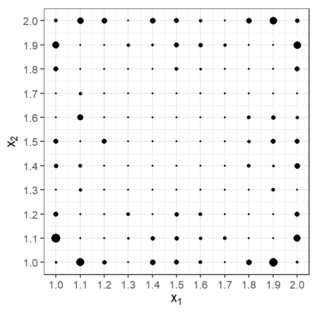
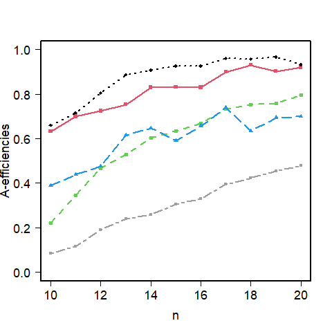
Figure 6: Graphs for Example 5. Left: discrete measure obtained by running linear programming algorithm for virtual noise representation for $n=10$. Right: A-efficiencies of exact designs with respect to optimal measure of virtual noise representation obtained by various methods for $n=10$ to $n=20$. The methods depicted are: R-VN (optimum: solid red line with squares, median: dashed green line with large dots), R-UNIF (optimum: long-dashed blue line with triangles, median: long-short-dashed grey line with small dots), BKSF (dotted black line with diamonds).

Efficiencies for Example 3

Figure 7 displays the D-efficiencies with respect to $\Phi\left\{M\!\left(\bar{\xi}\right)\right\}$ for Example 3 for $n=4$ to $n=40$.

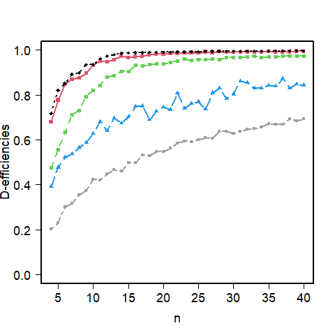
Figure 7: D-efficiencies for Example 3 for $n=4$ to $n=40$. The same line types, point symbols and colours are used for the respective methods as in the right panel of Figure 6.

References

- Atkinson et al. (2007) Atkinson, A. C., Donev, A. N., and Tobias, R. D. (2007), Optimum Experimental Designs, with SAS, no. 34 in Oxford Statistical Science Series, Oxford: Oxford University Press.
- Berkelaar et al. (2020) Berkelaar, M. et al. (2020), Interface to ‘Lp_solve’ v. 5.5 to Solve Linear/Integer Programs.
- Brimkulov et al. (1980) Brimkulov, U., Krug, G., and Savanov, V. (1980), “Numerical construction of exact experimental designs when the measurements are correlated,” Zavodskaya Laboratoria, 36, 435–442.
- Burclová and Pázman (2016) Burclová, K. and Pázman, A. (2016), “Optimal design of experiments via linear programming,” Statistical Papers, 57, 893–910.
- Dette et al. (2017) Dette, H., Konstantinou, M., and Zhigljavsky, A. (2017), “A new approach to optimal designs for correlated observations,” Annals of Statistics, 45, 1579–1608.
- Dette et al. (2016) Dette, H., Pepelyshev, A., and Zhigljavsky, A. (2016), “Optimal designs in regression with correlated errors,” The Annals of Statistics, 44, 113–152.
- Dette et al. (2019) — (2019), “The BLUE in continuous-time regression models with correlated errors,” The Annals of Statistics, 47, 1928–1959.
- Fedorov (1996) Fedorov, V. (1996), “Design of spatial experiments: Model fitting and prediction,” in Handbook of Statistics, eds. Ghosh, S. and Rao, C., Elsevier, vol. 13, pp. 515–553.
- Glatzer and Müller (1999) Glatzer, E. and Müller, W. G. (1999), “A comparison of optimum design algorithms for regressions with correlated observations,” in Probastat ’98, eds. Pázman, A. and Wimmer, G., Tatra Mountains Mathematical Publications, vol. 17, pp. 149 – 156.
- Goos and Jones (2011) Goos, P. and Jones, B. (2011), Optimal Design of Experiments: A Case Study Approach, Wiley.
- Harville (1997) Harville, D. A. (1997), Matrix Algebra From a Statistician’s Perspective, Springer.
- Kelley (1960) Kelley, J. E., J. (1960), “The Cutting-Plane Method for Solving Convex Programs,” Journal of the Society for Industrial and Applied Mathematics, 8, 703–712.
- Kiefer (1959) Kiefer, J. (1959), “Optimum Experimental Designs,” Journal of the Royal Statistical Society. Series B (Methodological), 21, 272–304.
- Mateu and Müller (2012) Mateu, J. and Müller, W. G. (2012), Spatio-temporal Design: Advances in Efficient Data Acquisition, Wiley.
- Morris (2010) Morris, M. (2010), Design of Experiments: An Introduction Based on Linear Models, Chapman and Hall/CRC.
- Müller and Pázman (2003) Müller, W. and Pázman, A. (2003), “Measures for designs in experiments with correlated errors,” Biometrika, 90, 423–434.
- Näther (1985) Näther, W. (1985), Effective Observation of Random Fields, Teubner.
- Pázman (2007) Pázman, A. (2007), “Criteria for optimal design of small-sample experiments with correlated observations,” Kybernetika, 43, 453–462.
- Pázman and Müller (1998) Pázman, A. and Müller, W. G. (1998), “A new interpretation of design measures,” in MODA 5 — Advances in Model-Oriented Data Analysis and Experimental Design, eds. Atkinson, A., Pronzato, L., and Wynn, H., Physica-Verlag HD, pp. 239–246.
- Pázman and Müller (2010) — (2010), “A note on the relationship between two approaches to optimal design under correlation,” in mODa 9 – Advances in Model-Oriented Design and Analysis, eds. Giovagnoli, A., Atkinson, A., Torsney, B., and May, C., Physica-Verlag HD, pp. 145–148.
- Pronzato and Pázman (2013) Pronzato, L. and Pázman, A. (2013), Design of Experiments in Nonlinear Models: Asymptotic Normality, Optimality Criteria and Small-Sample Properties, Lecture Notes in Statistics, Springer.
- Pukelsheim (2006) Pukelsheim, F. (2006), Optimal design of experiments, SIAM/Society for Industrial and Applied Mathematics.
- R Core Team (2020) R Core Team (2020), R: A Language and Environment for Statistical Computing, R Foundation for Statistical Computing, Vienna, Austria.
- Rasmussen and Williams (2005) Rasmussen, C. and Williams, C. (2005), Gaussian Processes for Machine Learning, Adaptive Computation and Machine Learning series, The MIT Press.
- Rockafellar (1970) Rockafellar, R. T. (1970), Convex Analysis, Princeton University Press.
- Sacks and Ylvisaker (1966) Sacks, J. and Ylvisaker, D. (1966), “Designs for regression problems with correlated errors,” The Annals of Mathematical Statistics, 37, 66–89.
- Uciński (2020) Uciński, D. (2020), “D-optimal sensor selection in the presence of correlated measurement noise,” Measurement, 164, 107873.
- Waite and Woods (2020) Waite, T. W. and Woods, D. C. (2020), “Minimax efficient random experimental design strategies with application to model-robust design for prediction,” Journal of the American Statistical Association, 1–36, publisher: Taylor & Francis _eprint: https://doi.org/10.1080/01621459.2020.1863221.
- Zhigljavsky et al. (2010) Zhigljavsky, A., Dette, H., and Pepelyshev, A. (2010), “A new approach to optimal design for linear models with correlated observations,” Journal of the American Statistical Association, 105, 1093–1103.