Multi-Mixed Fractional Brownian Motions and Orstein–Uhlenbeck Processes

Abstract.

We study the so-called multi-mixed fractional Brownian motions (mmfBm) and multi-mixed fractional Ornstein–Ulhenbeck (mmfOU) processes. These processes are constructed by mixing by superimposing (infinitely many) independent fractional Brownian motions (fBm) and fractional Ornstein–Uhlenbeck processes (fOU), respectively. We prove their existence as $L^{2}$ processes and study their path properties, viz. long-range and short-range dependence, Hölder continuity, $p$-variation, and conditional full support.

1. Introduction and Preliminaries

The fractional Brownian motion (fBm) $B^{H}$, with parameter $H\in(0,1)$ called the Hurst index, is the unique (up to a multiplicative constant) centered $H$-self-similar stationary-increment Gaussian process. The fBm was first studied in [15]. The name fractional Brownian motion comes from the influential article [18]. For further information of the fBm, see the monographs [5, 19]. The covariance of the fBm with Hurst index $H$ is given by

$$r_{H}(t,s)=\frac{1}{2}\left[t^{2H}+s^{2H}-|t-s|^{2H}\right].$$

For $H=1/2$ this process is well-known as the Brownian motion (Bm) or the Wiener process. As a stationary-increment process, the fBm admits the spectral density

(1.1) $$f_{H}(x)=\frac{\sin(\pi H)\Gamma(1+2H)}{2\pi}\,|x|^{1-2H},$$

where $\Gamma$ is the complete gamma function

$$\Gamma(\alpha)=\int_{0}^{\infty}t^{\alpha-1}\mathrm{e}^{-t}\,\mathrm{d}t,$$

see [22].

Let

$$\varrho_{H}(\delta;t)=\mathbb{E}\left[(B^{H}_{\delta}-B^{H}_{0})(B^{H}_{t+\delta}-B^{H}_{t})\right]$$

be the incremental autocovariance (with lag $\delta$) of the fBm. For $t\to\infty$ we have the power decay

$$\varrho_{H}(\delta;t)\sim H(2H-1)\delta^{2}t^{2H-2}.$$

This means that the increments of fBm, called the fractional Gaussian noise (fGn), are positively correlated and long-range dependent of $H>\frac{1}{2}$. For $H<\frac{1}{2}$ they are negatively correlated and short-range dependent.

In the Bm case $H=\frac{1}{2}$ we have independent increments, i.e., no dependence:

$$\varrho_{\frac{1}{2}}(\delta;t)=0.$$

A process $X$ is (locally) Hölder continuous with exponent $H$ if

$$\sup_{t,s\in[0,T]}\frac{|X_{t}-X_{s}|}{|t-s|^{H}}<\infty$$

The Hölder index of a process $X$ is

$$\mathrm{Hol}_{T}(X)=\sup\left\{H>0\,;\,\sup_{t,s\in[0,T]}\frac{|X_{t}-X_{s}|}{|t-s|^{H}}<\infty\right\}$$

The fBm has almost surely locally Hölder continuous paths with any order $H-\varepsilon$ for any $\varepsilon>0$, but not with order $H$. This follows, e.g., from Theorem 1 of [1]. Consequenlty, $\mathrm{Hol}(B^{H})=H$.

In addition to Hölder continuity, we have the equidistant $p$-variation as a measure of the path regularity. For a process $X$ and $p\in[1,\infty)$ for the equidistant partitions $\pi_{n}:=\{t_{k}=\frac{k}{n}T:k=0,1,\ldots,n\},$ consider the limit in probability

$$V^{p}_{T}(X):=\lim_{n\to\infty}\sum_{k=1}^{n}|X_{t_{k}}-X_{t_{k-1}}|^{p}.$$

If this limit is finite, it is called the equidistant $p$-variation on $[0,T]$ of $X$. The equidistant $p$-variation index of a process $X$ is

$$\mathrm{var}_{T}(X)=\sup\left\{p\,;\,V_{T}^{p}(X)<\infty\right\}.$$

For the fBm we have

$$V^{p}_{T}(B^{H})=\left\{\begin{array}[]{lll}\infty&;&pH<1\\ T\mu_{p}&;&pH=1\\ 0&;&pH>1\end{array}\right.$$

where $\mu_{p}$ is the $p$th moment of a standard Gaussian random variable, see [8, 9]. Consequently, $\mathrm{var}_{T}(B^{H})=1/H$.

While the fBm has been proposed as a model for financial time series, modeling with it makes arbitrage possible, see [3]. To eliminate this problem, a generalization called mixed fractional Brownian motion (mfBm) was introduced in [6]. This is the mixture model

$$M^{a,b}=aB+bB^{H},$$

where $a,b\in\mathbb{R}$ and $B$ is a standard Brownian motion (Bm) independent of the fBm $B^{H}$. If $H>1/2$, the mfBm has the path roughness governed by the Bm part and the long-range dependence governed by the fBm part. Hence, e.g., in pricing of financial derivatives the corresponding mixed Black–Scholes model yields the same option prices as the standard Brownian model, see [4].

A natural generalization of the mfBm is to consider two (or $n$) independent fBm mixtures, see [17]. In this paper, we study an independent infinite-mixture generalization that we call the multi-mixed fractional Brownian motion (mmfBm) with parameters $\sigma_{k}$, $H_{k}$, $k\in\mathbb{N}$:

$$M=\sum_{k=1}^{\infty}\sigma_{k}B^{H_{k}},$$

where $B^{H_{k}}$’s are independent fBm’s with Hurst indices $H_{k}\in(0,1)$, and $\sigma_{k}$’s are positive volatility constants satisfying $\sum_{k=1}^{\infty}\sigma_{k}^{2}<\infty$.

For other kinds of generalizations of the fBm, see e.g. [12, 16, 20, 21].

The fractional Ornstein–Uhlenbeck process (fOU) $U^{\lambda,H}$, with parameters $\lambda>0$ and $H\in(0,1)$ is the stationary solution of the Langevin equation

$$\mathrm{d}U^{\lambda,H}_{t}=-\lambda U^{\lambda,H}_{t}\mathrm{d}t+\mathrm{d}B^{H}_{t},$$

which is given by

$$U^{\lambda,H}_{t}=\int_{-\infty}^{t}\mathrm{e}^{-\lambda(t-s)}\,\mathrm{d}B^{H}_{s},$$

where $(B^{H}_{s})_{s\leq 0}$ is an independent copy of the fBm $(B^{H}_{s})_{s\geq 0}$, see [7]. Note that the Langevin equation and its solution can be understood via integration-by-parts. As a stationary process, the fOU admits the spectral density

(1.2) $$f_{\lambda,H}(x)=\frac{f_{H}(x)}{x^{2}+\lambda^{2}},$$

where $f_{H}$ is the spectral density of the driving fBm (1.1), see [2]. Denote, for $\alpha\in(-1,0)\cup(0,1)$

(1.3) $${\gamma}_{\alpha}(x) = \frac{1}{\Gamma(\alpha)}\int_{0}^{x}s^{\alpha-1}\mathrm{e}^{s}\,\mathrm{d}s,$$

(1.4) $${\Gamma}_{\alpha}(x) = \frac{1}{\Gamma(\alpha)}\int_{x}^{\infty}s^{\alpha-1}\mathrm{e}^{-s}\,\mathrm{d}s,$$

and ${\gamma}_{0}(x)=1$, ${\Gamma}_{0}(x)=0$. The autocovariance function of the fOU process can be written as

(1.5) $$\rho_{\lambda,H}(t)=\frac{\Gamma(1+2H)}{4}\frac{\mathrm{e}^{-\lambda t}}{\lambda^{2H}}\bigg{\{}1+{\gamma}_{2H-1}(\lambda t)+\mathrm{e}^{2\lambda t}{\Gamma}_{2H-1}(\lambda t)\bigg{\}},$$

see Proposition 2.4 below. For $H=\frac{1}{2}$ we recover the well-known Bm case

$$\rho_{\lambda,\frac{1}{2}}(t)=\frac{\mathrm{e}^{-\lambda t}}{2\lambda}.$$

For $t\to\infty$ we have the power decay

$$\rho_{\lambda,H}(t)=\frac{1}{2}\sum_{n=1}^{N}\lambda^{-2n}\left(\prod_{j=0}^{2n-1}(2H-j)\right)t^{2H-2n}+O(t^{2H-2N-2}),$$

for $N=1,2,\ldots$, i.e., the fOU process with $H>\frac{1}{2}$ is long-range dependent, and for $H\leq\frac{1}{2}$ it is short-range dependent, see [7].

The Hölder index and the $p$-variation $p$-variation index of fOU is the same as for the fBm: $\mathrm{Hol}_{T}(U^{\lambda,H})=\mathrm{Hol}_{T}(B^{H})=H$ and $\mathrm{var}_{T}(U^{\lambda,H})=\mathrm{var}_{T}(B^{H})=1/H$. These results follow e.g. from our Theorem 4.1 and Theorem 5.1.

In this paper we study the multi-mixed fractional Ornstein–Uhlenbeck process (mmfOU) with parameters $\lambda>0$ and $\sigma_{k}$, $H_{k}$, $k\in\mathbb{N}$, that is defined naturally as the stationary solution of Langevin equation with mmfBm as the driving noise:

$$\mathrm{d}U_{t}=-\lambda U_{t}\,\mathrm{d}t+\mathrm{d}M_{t},$$

with

$$U_{0}=\int_{-\infty}^{0}\mathrm{e}^{\lambda s}\,\mathrm{d}M_{s},$$

where $(M_{s})_{s\leq 0}$ is an independent copy of the mmfBm.

The rest of the paper is organized as follows. In Section 2 we define the multi-mixed fractional Brownian motions (mmfBm) and the associated multi-mixed fractional Ornstein–Uhlenbeck (mmfOU) processes, prove their existence in $L^{2}(\Omega\times[0,T])$, and provide their basic properties. The long-range dependence of these processes are what we studied in Section 3 In Section 4 we analyze the Hölder continuity and $p$-variation of mmfBm’s and mmfOU processes. The $p$-variation of these processes are calculated in Section 5 In Section 6 we show that the mmfBm’s and mmfOU processes have the conditional full support property. Finally, In Section 7 some simulated path of these processes are given.

2. Definitions and Basic Properties

Definition 2.1.

Let $\sigma_{k}$, $k\in\mathbb{N}$, satisfy

(2.1) $$\sum_{k=1}^{\infty}\sigma_{k}^{2}<\infty,$$

and let $H_{k}$, $k\in\mathbb{N}$, satisfy

$$H_{k}\neq H_{l}\mbox{ for }k\neq l,$$

(2.2) $$H_{\inf}=\inf_{k\in\mathbb{N}}H_{k}>0$$

$$H_{\sup}=\sup_{k\in\mathbb{N}}H_{k}<1.$$

The multi-mixed fractional Brownian motion (mmfBm) is

$$M=\sum_{k=1}^{\infty}\sigma_{k}B^{H_{k}},$$

where $B^{H_{k}}$, $k\in\mathbb{N}$, are independent fBm’s.

The following proposition shows the existence of the mmfBm.

Proposition 2.1.

The mmfBm $M$ exist as a random function taking values in $L^{2}(\Omega\times[0,T])$ for all $T>0$.

Proof.

Let $M^{n}=\sum_{k=1}^{n}\sigma_{k}B^{H_{k}}.$ Clearly $M^{n}$ takes values in $L^{2}(\Omega\times[0,T])$. Let $n,m\in\mathbb{N}$ with $n>m$. Then

$${\|M^{n}-M^{m}\|}^{2}_{L^{2}(\Omega\times[0,T])} = \int_{0}^{T}\mathbb{E}\left[(M_{t}^{n}-M_{t}^{m})^{2}\right]\,\mathrm{d}t$$

$$= \int_{0}^{T}\mathbb{E}\left[\left(\sum_{k=m+1}^{n}\sigma_{k}B^{H_{k}}_{t}\right)^{2}\right]\,\mathrm{d}t$$

$$= \sum_{k=m+1}^{n}\int_{0}^{T}\sigma_{k}^{2}\mathbb{E}\left[(B_{t}^{H_{k}})^{2}\right]\,\mathrm{d}t$$

$$= \sum_{k=m+1}^{n}\int_{0}^{T}\sigma_{k}^{2}t^{2H_{k}}\,\mathrm{d}t$$

$$= \sum_{k=m+1}^{n}\sigma_{k}^{2}\frac{T^{1+2H_{k}}}{1+2H_{k}}$$

$$\leq \sum_{k=m+1}^{n}\sigma_{k}^{2}\,\max\left\{1,T^{3}\right\},$$

which shows that the sequence $(M^{n})_{n\in\mathbb{N}}$ is Cauchy. Thus $M^{n}\to M$ in $L^{2}(\Omega\times[0,T])$ showing the existence. ∎

In the same way we see that the mmfBm $(M_{t})_{t\geq 0}$ exist in the sense that $M^{n}_{t}\to M_{t}$ in $L^{2}(\Omega)$ for all $t\geq 0$.

The following is now obvious:

Proposition 2.2.

The mmfBm has stationary increments, its covariance function is

(2.3) $$r(t,s)=\sum_{k=1}^{\infty}\sigma_{k}^{2}r_{H_{k}}(s,t)=\frac{1}{2}\sum_{k=1}^{\infty}\sigma_{k}^{2}\left[|t|^{2H_{k}}+|s|^{2H_{k}}-|t-s|^{2H_{k}}\right],$$

and it admits the spectral density

(2.4) $$f(x)=\sum_{k=1}^{\infty}\sigma_{k}^{2}f_{H_{k}}(x)=\sum_{k=1}^{\infty}\frac{\sin(\pi H_{k})\Gamma(1+2H_{k})}{2\pi}\sigma_{k}^{2}|x|^{1-2H_{k}}.$$

Definition 2.2.

The multi-mixed fractional Ornstein–Uhlenbeck process (mmfOU) $U$ with parameter $\lambda>0$, is the stationary solution of the Langevin equation

(2.5) $$\mathrm{d}U_{t}=-\lambda U_{t}\mathrm{d}t+\mathrm{d}M_{t},$$

where the equation is understood in the integration-by-parts sense.

Proposition 2.3.

On $L^{2}(\Omega\times[0,T])$, the mmfOU can be represented as the integral

$$U_{t}=\mathrm{e}^{-\lambda t}\xi+\int_{0}^{t}\mathrm{e}^{-\lambda(t-s)}\,\mathrm{d}M_{s},$$

where the integral is understood in the integration-by-parts sense, and

$$\xi=\int_{-\infty}^{0}\mathrm{e}^{\lambda s}\,\mathrm{d}M_{s},$$

where $(M_{s})_{s\leq 0}$ is an independent copy of the mmfBm $(M_{s})_{s\geq 0}$.

Proof.

Let $M^{n}=\sum_{k=1}^{n}\sigma_{k}B^{H_{k}}$. Then, the stationary solution of the Langevin equation

$$\mathrm{d}U^{n}_{t}=-\lambda U^{n}_{t}\mathrm{d}t+\mathrm{d}M^{n}_{t},$$

is given by

$$U^{n}_{t}=\mathrm{e}^{-\lambda t}\xi_{n}+\int_{0}^{t}\mathrm{e}^{-\lambda(t-s)}\,\mathrm{d}M^{n}_{s},$$

where

$$\xi_{n}=\int_{-\infty}^{0}\mathrm{e}^{\lambda s}\,\mathrm{d}M^{n}_{s}.$$

Then, with integration-by-parts

$$\int_{0}^{t}\mathrm{e}^{\lambda s}\,\mathrm{d}M^{n}_{s}=\mathrm{e}^{\lambda t}M^{n}_{t}-\lambda\int_{0}^{t}\mathrm{e}^{\lambda s}M^{n}_{s}\,\mathrm{d}s\ \to\ \mathrm{e}^{\lambda t}M_{t}-\lambda\int_{0}^{t}\mathrm{e}^{\lambda s}M_{s}\,\mathrm{d}s=\int_{0}^{t}\mathrm{e}^{\lambda s}\,\mathrm{d}M_{s},$$

because $M^{n}\to M$ in $L^{2}(\Omega\times[0,T])$. With the same arguments $\xi_{n}\to\xi$ in $L^{2}(\Omega)$. This yields $U^{n}\to U$ in $L^{2}(\Omega\times[0,T])$. ∎

The following technical lemma is used to calculate spectral densities.

Lemma 2.1.

For $0\neq p\in(-1,1),\,\lambda>0,\,t>0$

(2.6) $$\int_{-\infty}^{\infty}\mathrm{e}^{\mathrm{i}tx}\frac{|x|^{p}}{\lambda^{2}+x^{2}}\,\mathrm{d}x=\frac{\pi\mathrm{e}^{-\lambda t}}{2\cos(\frac{p\pi}{2})\lambda^{1-p}}\left\{1+\gamma_{-p}(\lambda t)+\mathrm{e}^{2\lambda t}\Gamma_{-p}(\lambda t)\right\},$$

where $\gamma_{-p}$ and $\Gamma_{-p}$ are given by (1.3) and (1.4).

Proof.

Recall that for the Fourier transform

$$\mathscr{F}(f)(x)=\frac{1}{\sqrt{2\pi}}\int_{-\infty}^{\infty}\mathrm{e}^{-\mathrm{i}tx}f(t)\,\mathrm{d}t,$$

we have the convolution theorem

(2.7) $$\int_{-\infty}^{\infty}\mathrm{e}^{\mathrm{i}tx}\mathscr{F}(f)(x)\mathscr{F}(g)(x)\,\mathrm{d}x=\int_{-\infty}^{\infty}f(t-\xi)g(\xi)\,\mathrm{d}\xi.$$

Moreover, we have

(2.8) $$\mathscr{F}\left(e^{-\lambda|t|}\right)=\sqrt{\frac{2}{\pi}}\cdot\frac{\lambda}{\lambda^{2}+x^{2}},$$

(2.9) $$\mathscr{F}\left(|t|^{\alpha}\right)=\sqrt{\frac{2}{\pi}}\cdot\Gamma(\alpha+1)\cos\left(\frac{(\alpha+1)\pi}{2}\right)|x|^{-(\alpha+1)}.$$

The first formula (2.8) is valid for $\lambda>0$. The second formula (2.9) is valid for $-1<\alpha<0$. For $-2<\alpha<-1$, because of the function $|t|^{\alpha}$, some singular terms arise at the origin. Nevertheless, it admits a unique meromorphic extension as a tempered distribution, also denoted $|t|^{\alpha}$ as a homogeneous distribution on all real line $\mathbb{R}$ including the origin (see [11]). So, we use that extension and formula (2.9) will be valid for all $-1\neq\alpha\in(-2,0)$. So, using $f(t)=e^{-\lambda|t|}$ and $g(t)=|t|^{\alpha}$ in (2.7) we obtain

$$\frac{2}{\pi}\cdot\Gamma(\alpha+1)\cos\left(\frac{(\alpha+1)\pi}{2}\right)\lambda\int_{-\infty}^{\infty}\mathrm{e}^{itx}\frac{|x|^{-(\alpha+1)}}{\lambda^{2}+x^{2}}\,\mathrm{d}x$$

$$= \int_{-\infty}^{\infty}|\xi|^{\alpha}\mathrm{e}^{-\lambda|t-\xi|}\,\mathrm{d}\xi$$

$$= \int_{-\infty}^{0}(-\xi)^{\alpha}\mathrm{e}^{-\lambda(t-\xi)}\,\mathrm{d}\xi+\int_{0}^{t}\xi^{\alpha}\mathrm{e}^{-\lambda(t-\xi)}\,\mathrm{d}\xi+\int_{t}^{\infty}\xi^{\alpha}\mathrm{e}^{-\lambda(\xi-t)}\,\mathrm{d}\xi$$

$$= \frac{\mathrm{e}^{-\lambda t}}{\lambda^{(\alpha+1)}}\int_{0}^{\infty}u^{\alpha}\mathrm{e}^{-u}\,\mathrm{d}u+\frac{\mathrm{e}^{-\lambda t}}{\lambda^{(\alpha+1)}}\int_{0}^{\lambda t}u^{\alpha}\mathrm{e}^{u}\,\mathrm{d}u+\frac{\mathrm{e}^{\lambda t}}{\lambda^{(\alpha+1)}}\int_{\lambda t}^{\infty}u^{\alpha}\mathrm{e}^{-u}\,\mathrm{d}u$$

$$= \frac{\mathrm{e}^{-\lambda t}\Gamma(\alpha+1)}{\lambda^{(\alpha+1)}}\left\{1+\gamma_{(\alpha+1)}(\lambda t)+\mathrm{e}^{2\lambda t}\Gamma_{(\alpha+1)}(\lambda t)\right\}.$$

Now, choosing $p=-(\alpha+1)$ proves (2.6). ∎

It follows from Lemma 2.1 that:

Proposition 2.4.

The covariance function of the fOU is

(2.10) $$\rho_{\lambda,H}(t)=\mathbb{E}[U^{\lambda,H}_{s}U^{\lambda,H}_{s+t}]=\frac{\Gamma(1+2H)}{4}\frac{\mathrm{e}^{-\lambda t}}{\lambda^{2H}}\bigg{\{}1+{\gamma}_{2H-1}(\lambda t)+\mathrm{e}^{2\lambda t}{\Gamma}_{2H-1}(\lambda t)\bigg{\}}.$$

Proposition 2.5.

The covariance function of the mmfOU is

(2.11) $$\rho_{\lambda}(t)=\mathbb{E}[U_{s}U_{s+t}]=\sum_{k=1}^{\infty}\sigma_{k}^{2}\frac{\Gamma(1+2H_{k})\mathrm{e}^{-\lambda t}}{4\lambda^{2H_{k}}}\bigg{\{}1+\gamma_{2H_{k}-1}(\lambda t)+\mathrm{e}^{2\lambda t}\Gamma_{2H_{k}-1}(\lambda t)\bigg{\}},$$

and it admits the spectral density

(2.12) $$f_{\lambda}(x)=\sum_{k=1}^{\infty}\sigma_{k}^{2}\frac{\sin(\pi H_{k})\Gamma(1+2H_{k})}{2\pi}\frac{|x|^{1-2H_{k}}}{x^{2}+\lambda^{2}}.$$

Proof.

Let $U^{n}$ be like in the proof of Proposition 2.3, then

$$f_{\lambda,n}(x)=\sum_{k=1}^{n}\sigma_{k}^{2}\frac{\sin(\pi H_{k})\Gamma(1+2H_{k})}{2\pi}\frac{|x|^{1-2H_{k}}}{x^{2}+\lambda^{2}},$$

and $f_{\lambda,n}(x)\to f_{\lambda}(x)$ because $U^{n}\to U$ in $L^{2}(\Omega\times[0,T])$. This proves (2.12). Similarly, (2.11) follows by Proposition 2.4. ∎

Remark 2.1.

Proposition 2.4 represents the covariance function $\rho_{\lambda,H}(t)$ in a form involving special functions. However, these special complex functions are usually not suitable for numerical computations. For example,in [2], Lemma B.1, the following representation was used for $H>\frac{1}{2}$

$$\rho_{\lambda,H}(t) = H\Gamma(2H)\frac{e^{-\lambda t}}{\lambda^{2H}}\left\{\frac{1+e^{2\lambda t}}{2}-\frac{\lambda}{\Gamma(2H-1)}I_{\lambda,H}(t)\right\},$$

$$I_{\lambda,H}(t) = \int_{0}^{t}\int_{0}^{\lambda v}e^{2\lambda v}e^{-s}s^{2H-2}\,\mathrm{d}s\mathrm{d}v.$$

the double integral above seems reasonable enough, but yields slow numerical calculation in practice. This can be remedied by calculating the inner integral as follows:

$$I_{\lambda,H}(t) = \int_{0}^{\lambda t}\int_{s/{\lambda}}^{t}e^{2\lambda v}e^{-s}s^{2H-2}\,\mathrm{d}s\mathrm{d}v$$

$$= \frac{1}{2\lambda}\int_{0}^{\lambda t}s^{2H-2}(e^{2\lambda t-s}-e^{s})\,\mathrm{d}s$$

$$= \frac{e^{\lambda t}}{\lambda}\int_{0}^{\lambda t}s^{2H-2}\sinh(\lambda t-s)\,\mathrm{d}s.$$

Consequently,

$$\rho_{\lambda,H}(t)=\frac{\Gamma(2H+1)}{2\lambda^{2H}}\bigg{\{}\cosh(\lambda t)-\frac{1}{\Gamma(2H-1)}\int_{0}^{\lambda t}s^{2H-2}\sinh(\lambda t-s)\,ds\bigg{\}},$$

For the case $H<1/2$ we use the following developed version of Lemma 5.1 in [13] for $\alpha>-1$. The proof is similar.

Lemma 2.2.

For $\alpha>-1$

$$\int_{0}^{\infty}\int_{0}^{\infty}\mathrm{e}^{-(x+y)}|x-y|^{\alpha}\,\mathrm{d}x\mathrm{d}y=\Gamma(\alpha+1).$$

Theorem 2.1.

For the fOU process $U^{\lambda,H}$. We have

$$\rho_{\lambda,H}(t)=\frac{\Gamma(2H+1)}{2\lambda^{2H}}\,\bigg{\{}\cosh(\lambda t)-\frac{1}{\Gamma(2H)}\int_{0}^{\lambda t}s^{2H-1}\cosh(\lambda t-s)\,ds\bigg{\}},$$

and so for mmfOU process we have

$$\rho_{\lambda}(t)=\sum_{k=0}^{\infty}\sigma_{k}^{2}\frac{\Gamma(2H_{k}+1)}{2\lambda^{2H_{k}}}\,\bigg{\{}\cosh(\lambda t)-\frac{1}{\Gamma(2H_{k})}\int_{0}^{\lambda t}s^{2H_{k}-1}\cosh(\lambda t-s)\,ds\bigg{\}}.$$

Proof.

For $H=1/2$ the right hand side of (2.1) is $\mathrm{e}^{-\lambda t}/2\lambda$ wich is equal to the outocovariance of the classical Ornstein–Uhlenbeck process with respect to the standard Brownian motion. For $H>1/2$, we obtain (2.1) from (2.1) via integration by part. To prove it for $H<1/2$, we will apply the same approach of the proof of Lemma B.1 in [2]

$$\rho_{\lambda,H}(t)= \ \mathbb{E}[U^{\lambda,H}_{t}U^{\lambda,H}_{0}]$$

$$= \ \mathbb{E}\left[\int_{-\infty}^{0}\mathrm{e}^{\lambda u}\,\mathrm{d}B^{H}_{u}\int_{-\infty}^{t}\mathrm{e}^{-\lambda(t-v)}\,\mathrm{d}B^{H}_{v}\right]$$

$$= \ \mathrm{e}^{-\lambda t}\bigg{\{}\mathbb{V}ar(U^{\lambda,H}_{0})+\mathbb{E}\bigg{[}\int_{-\infty}^{0}\mathrm{e}^{\lambda u}\,\mathrm{d}B^{H}_{u}\int_{0}^{t}\mathrm{e}^{\lambda v}\,\mathrm{d}B^{H}_{v}\bigg{]}\bigg{\}}.$$

To obtain the term $\mathbb{V}ar(U^{\lambda,H}_{0})$ in a close form, [2] referred to Lemma 5.2 in [13]; however, it was only obtained for $H\geq 1/2$, and so we need to extend their result for $H<1/2$.

Since

$$U^{\lambda,H}_{0}=\int_{-\infty}^{0}\mathrm{e}^{\lambda u}\,\mathrm{d}B^{H}_{u}=-\lambda\int_{-\infty}^{0}\mathrm{e}^{\lambda u}B^{H}_{u}\,\mathrm{d}u,$$

we have

$$\mathbb{V}ar(U^{\lambda,H}_{0})= \mathbb{V}ar\left[-\lambda\int_{-\infty}^{0}\mathrm{e}^{\lambda u}B^{H}_{u}\,\mathrm{d}u\right]$$

$$= \ \lambda^{2}\mathbb{V}ar\left[\int_{0}^{\infty}\mathrm{e}^{-\lambda u}B^{H}_{u}\,\mathrm{d}u\right]$$

$$= \ \lambda^{2}\mathbb{E}\left[\left(\int_{0}^{\infty}\mathrm{e}^{-\lambda u}B^{H}_{u}\,\mathrm{d}u\right)^{2}\right]$$

$$= \ \lambda^{2}\mathbb{E}\left[\int_{0}^{\infty}\int_{0}^{\infty}\mathrm{e}^{-\lambda(u+v)}B^{H}_{u}B^{H}_{v}\,\mathrm{d}u\mathrm{d}v\right]$$

$$= \ \frac{\lambda^{2}}{2}\int_{0}^{\infty}\int_{0}^{\infty}\mathrm{e}^{-\lambda(u+v)}\cdot\Big{\{}u^{2H}+v^{2H}-|u-v|^{2H}\Big{\}}\,\mathrm{d}u\mathrm{d}v$$

$$= \ \frac{\lambda^{2}}{2}\bigg{\{}2\left(\int_{0}^{\infty}\mathrm{e}^{-\lambda u}\,\mathrm{d}u\right)\left(\int_{0}^{\infty}\mathrm{e}^{-\lambda v}v^{2H}\,\mathrm{d}v\right)-\int_{0}^{\infty}\int_{0}^{\infty}\mathrm{e}^{-\lambda(u+v)}|u-v|^{2H}\,\mathrm{d}u\mathrm{d}v\bigg{\}},$$

Now choosing $x=\lambda u,\,y=\lambda v$ and Lemma 2.2 we have

$$\mathbb{V}ar(U^{\lambda,H}_{0}) =\frac{\lambda^{-2H}}{2}\bigg{\{}2\int_{0}^{\infty}\mathrm{e}^{-y}y^{2H}\,\mathrm{d}y-\int_{0}^{\infty}\int_{0}^{\infty}\mathrm{e}^{-(x+y)}|x-y|^{2H}\,\mathrm{d}x\mathrm{d}y\bigg{\}}$$

$$=\frac{\lambda^{-2H}}{2}\Big{[}2\Gamma(2H+1)-\Gamma(2H+1)\Big{]}$$

(2.13) $$=\lambda^{-2H}H\Gamma(2H).$$

On the other hand, as in Lemma 2.1 in [7] and the proof of Lemma B.1 in [2], using formula

$$\gamma_{\ell}(z,x)=\frac{\gamma_{\ell}(z+1,x)+x^{z}\mathrm{e}^{-x}}{z},$$

where $\gamma_{\ell}$ is the well-known lower Gamma function, for $H<1/2$ we have

(2.14) $$\mathbb{E}\left[\int_{-\infty}^{0}\mathrm{e}^{\lambda u}\,\mathrm{d}B^{H}_{u}\int_{0}^{t}\mathrm{e}^{\lambda v}\,\mathrm{d}B^{H}_{v}\right]$$

$$=H(2H-1)\int_{-\infty}^{0}\int_{0}^{t}\mathrm{e}^{-\lambda(u+v)}|u-v|^{2H-2}\,\mathrm{d}u\mathrm{d}v$$

$$=\mathbb{V}ar(U^{\lambda,H}_{0})\bigg{\{}\frac{\mathrm{e}^{2\lambda t}-1}{2}-\frac{\lambda}{\Gamma(2H-1)}\int_{0}^{t}\mathrm{e}^{2\lambda v}\int_{0}^{\lambda v}\mathrm{e}^{-s}s^{2H-2}\,\mathrm{d}s\mathrm{d}v\bigg{\}}$$

$$=\mathbb{V}ar(U^{\lambda,H}_{0})\bigg{\{}\frac{\mathrm{e}^{2\lambda t}-1}{2}-\frac{\lambda}{\Gamma(2H-1)}\int_{0}^{t}\mathrm{e}^{2\lambda v}\gamma_{\ell}(2H-1,\lambda v)\,\mathrm{d}v\bigg{\}}$$

$$=\mathbb{V}ar(U^{\lambda,H}_{0})\bigg{\{}\frac{\mathrm{e}^{2\lambda t}-1}{2}-\frac{\lambda}{\Gamma(2H)}\int_{0}^{t}\mathrm{e}^{2\lambda v}\gamma_{\ell}(2H,\lambda v)\,\mathrm{d}v-\frac{\lambda^{2H}}{\Gamma(2H)}\int_{0}^{t}\mathrm{e}^{\lambda v}v^{2H-1}\,\mathrm{d}v\bigg{\}}$$

$$=\mathbb{V}ar(U^{\lambda,H}_{0})\bigg{\{}\frac{\mathrm{e}^{2\lambda t}-1}{2}-\frac{\lambda}{\Gamma(2H)}\int_{0}^{t}\mathrm{e}^{2\lambda v}\int_{0}^{\lambda v}\mathrm{e}^{-s}s^{2H-1}\,\mathrm{d}s\mathrm{d}v-\frac{\lambda^{2H}}{\Gamma(2H)}\int_{0}^{t}\mathrm{e}^{\lambda v}v^{2H-1}\,\mathrm{d}v\bigg{\}}.$$

Using (2.13) and (2.14), with similar arguments as we did for (2.1) we obtain (2.1). ∎

3. Long-Range Dependence

The increments of fBm, the fGn, is a well-known stationary process, that is long-range dependent (LRD) if $H>1/2$, and short-range dependent (SRD) in $H<\frac{1}{2}$ Motivated with this, we consider the LRD of the increments the of mmfBm.

For a lag $\delta$ and a process $X$ we denote $\Delta_{\delta}X_{t}=X_{t+\delta}-X_{t}.$ Then

$$\Delta_{\delta}M_{t}=\sum_{k=1}^{\infty}\sigma_{k}\Delta_{\delta}B^{H_{k}}_{t}$$

is stationary and its autocovariance function is denoted by

$$\varrho(\delta;t)=\mathbb{E}\big{[}\Delta_{\delta}M_{s+t}\Delta_{\delta}M_{s}\big{]},$$

Theorem 3.1.

For $t\to\infty$

(3.1) $$\varrho(\delta;t)\sim\delta^{2}\sum_{k=1}^{\infty}\sigma_{k}^{2}H_{k}(2H_{k}-1)t^{2H_{k}-2}=O(t^{2H_{\sup}-2}).$$

So the mmfBm increment process $\Delta_{\delta}M_{t}$ is LRD if and only if $H_{k}>1/2$ for some $k\geq 0$.

Proof.

By using the generalized binomial theorem

(3.2) $$\varrho(\delta;t) = \frac{1}{2}\sum_{k=1}^{\infty}\sigma_{k}^{2}\Big{\{}(t+\delta)^{2H_{k}}+(t-\delta)^{2H_{k}}-2t^{2H_{k}}\Big{\}}$$

$$= \frac{1}{2}\sum_{k=1}^{\infty}\sigma_{k}^{2}t^{2H_{k}}\Bigg{\{}\Big{(}1+\frac{\delta}{t}\Big{)}^{2H_{k}}+\Big{(}1-\frac{\delta}{t}\Big{)}^{2H_{k}}-2\Bigg{\}}$$

$$= \frac{1}{2}\sum_{k=1}^{\infty}\sigma_{k}^{2}t^{2H_{k}}\Bigg{\{}\sum_{r=0}^{\infty}\binom{2H_{k}}{r}\Big{(}\frac{\delta}{t}\Big{)}^{r}+\sum_{r=0}^{\infty}\binom{2H_{k}}{r}(-1)^{r}\Big{(}\frac{\delta}{t}\Big{)}^{r}-2\Bigg{\}}$$

$$\sim \delta^{2}\sum_{k=1}^{\infty}\sigma_{k}^{2}H_{k}(2H_{k}-1)t^{2H_{k}-2}.$$

Since

$$\sigma_{k}^{2}H_{k}(2H_{k}-1)t^{2H_{k}-2}\leq\sigma_{k}^{2},$$

the series (3.2) is uniformly convergent. So we have

$$\lim_{t\to\infty}\sum_{k=1}^{\infty}\sigma_{k}^{2}H_{k}(2H_{k}-1)t^{2H_{k}-2}=\sum_{k=1}^{\infty}\lim_{t\to\infty}\sigma_{k}^{2}H_{k}(2H_{k}-1)t^{2H_{k}-2}.$$

This yields (3.1). ∎

To investigate LRD for the mmfOU process, we first need some lemmas.

The following theorem shows that similar to the mmfBm increment process, the long-range dependence of the mmfOU is governed by the long-range dependence of the largest Hurst index in the driving mmfBm.

Theorem 3.2.

For $t\to\infty$ and each $N=1,2,\ldots$

(3.3) $$\rho_{\lambda}(t)=\frac{1}{2}\sum_{k=1}^{\infty}\sum_{n=1}^{N}\sigma^{2}_{k}\lambda^{-2n}\left(\prod_{j=0}^{2n-1}(2H_{k}-j)\right)t^{2H_{k}-2n}+O(t^{2H_{\sup}-2N-2}).$$

So the mmfOU process $U$ is LRD if and only if $H_{k}>1/2$ for some $k\geq 0$.

Proof.

By the proof of Lemma 2.2 and Theorem 2.3 in [7]

$$\rho_{\lambda}(t)= \mathbb{E}\left[\int_{-\infty}^{0}\mathrm{e}^{\lambda u}\,\mathrm{d}M_{u}\int_{-\infty}^{t}\mathrm{e}^{-\lambda(t-v)}\,\mathrm{d}M_{v}\right]$$

$$= \mathrm{e}^{-\lambda t}\mathbb{E}\left[\int_{-\infty}^{0}\mathrm{e}^{\lambda u}\,\mathrm{d}M_{u}\int_{-\infty}^{1/\lambda}\mathrm{e}^{\lambda v}\,\mathrm{d}M_{v}\right]$$

$$+ \mathrm{e}^{-\lambda t}\sum_{i=1}^{\infty}\sigma_{i}^{2}H_{i}(2H_{i}-1)\int_{-\infty}^{0}\mathrm{e}^{\lambda u}\left(\int_{1/\lambda}^{t}\mathrm{e}^{\lambda v}(v-u)^{2H_{i}-2}\,\mathrm{d}v\right)\mathrm{d}u$$

$$= O(\mathrm{e}^{-\lambda t})+\frac{1}{2}\sum_{i=1}^{\infty}\sigma_{i}^{2}\frac{H_{i}(2H_{i}-1)}{\lambda^{2H_{i}}}\Bigg{\{}\mathrm{e}^{-\lambda t}\int_{1}^{\lambda t}\mathrm{e}^{y}y^{2H_{i}-2}\,\mathrm{d}y+\mathrm{e}^{\lambda t}\int_{\lambda t}^{\infty}\mathrm{e}^{-y}y^{2H_{i}-2}\,\mathrm{d}y\Bigg{\}}$$

$$\leq O(\mathrm{e}^{-\lambda t})+\frac{1}{2}\sum_{k=1}^{\infty}\sum_{n=1}^{N}\sigma^{2}_{k}\lambda^{-2n}\left(\prod_{j=0}^{2n-1}(2H_{k}-j)\right)t^{2H_{k}-2n}$$

$$+ \frac{1}{2}\sum_{k=1}^{\infty}\sigma_{k}^{2}\frac{\Big{|}H_{k}(2H_{k}-1)\cdots(2H_{k}-2-2N)\Big{|}}{\lambda^{2H_{k}}}\left[\mathrm{e}^{-\frac{\lambda t}{2}}+(1+2^{2H_{k}-2N-3})(\lambda t)^{2H_{k}-2N-3}\right].$$

Now, for $t\in[1,\infty)$

$$\sigma_{k}^{2} \frac{\Big{|}H_{k}(2H_{k}-1)\cdots(2H_{k}-2-2N)\Big{|}}{\lambda^{2H_{k}}}\,\mathrm{e}^{-\frac{\lambda t}{2}}<\Lambda_{N}\sigma_{k}^{2}$$

$$\sigma_{k}^{2} \frac{\Big{|}H_{k}(2H_{k}-1)\cdots(2H_{k}-2-2N)\Big{|}}{\lambda^{2H_{k}}}\,(1+2^{2H_{k}-2N-3})(\lambda t)^{2H_{k}-2N-3}<\Pi_{N}\sigma_{k}^{2},$$

where

$$\Lambda_{N} = H_{\sup}\frac{\max\Big{(}|2H_{\inf}-1|,|2H_{\sup}-1|\Big{)}}{\max\Big{(}\lambda^{2H_{\inf}},\lambda^{2H_{\sup}}\Big{)}}\Big{|}(2H_{\inf}-2)\cdots(2H_{\inf}-2-2N)\Big{|},$$

$$\Pi_{N} = H_{\sup}\frac{\max\Big{(}|2H_{\inf}-1|,|2H_{\sup}-1|\Big{)}}{\lambda^{2N+3}}\Big{|}(2H_{\inf}-2)\cdots(2H_{\inf}-2-2N)\Big{|}(1+2^{2H_{\sup}-2N-3}).$$

So, as $\sum_{k=1}^{\infty}\sigma_{k}^{2}<\infty$, the series in the right-hand side of the inequality (3) is uniformly convergent on $t\in[1,\infty)$. Hence

$$\lim_{t\to\infty}\sum_{k=1}^{\infty}\sigma_{k}^{2}\frac{\Big{|}H_{k}(2H_{k}-1)\cdots(2H_{k}-2-2N)\Big{|}}{\lambda^{2H_{k}}}\left[\mathrm{e}^{-\frac{\lambda t}{2}}+(1+2^{2H_{k}-2N-3})(\lambda t)^{2H_{k}-2N-3}\right]$$

$$=\sum_{k=1}^{\infty}\sigma_{k}^{2}\frac{\Big{|}H_{k}(2H_{k}-1)\cdots(2H_{k}-2-2N)\Big{|}}{\lambda^{2H_{k}}}\lim_{t\to\infty}\left[\mathrm{e}^{-\frac{\lambda t}{2}}+(1+2^{2H_{k}-2N-3})(\lambda t)^{2H_{k}-2N-3}\right].$$

This proves (3.3). ∎

4. Continuity

Theorem 4.1.

Both mmfBm and mmfOU have Hölder index $H_{\inf}$.

Proof.

For $\epsilon>0$ and $|t-s|<1$, the mmfBm satisfies

$$\mathbb{E}\Big{[}(M_{t}-M_{s})^{2}\Big{]}=\sum_{k=1}^{\infty}\sigma_{k}^{2}|t-s|^{2H_{k}}\leq\bigg{(}\sum_{k=1}^{\infty}\sigma_{k}^{2}\bigg{)}|t-s|^{2H_{\inf}-\epsilon}=C_{0}|t-s|^{2H_{\inf}-\epsilon},$$

where $C_{0}:=\sum_{k=1}^{\infty}\sigma_{k}^{2}>0$. Thus, Hölder continuity with exponent $H_{\inf}-\varepsilon$ follows from Theorem 1 of [1]. On the other hand, for some $j\geq 1$ we have $H_{\inf}\leq H_{j}<H_{\inf}+\epsilon$ and so the fBm $B^{H_{j}}$ is not $(H_{\inf}+\epsilon)$-Hölder continuous. Hence the process $M=\sigma_{j}B^{H_{j}}+\sum_{k\neq j}\sigma_{k}B^{H_{k}}$ is not $(H_{\inf}+\epsilon)$-Hölder continuous. This proves the claim for mmfBm.

For the mmfOU, we apply the Corollary 2 of [1]. That states that the stationary process $U$ is Hölder-continuous with any exponent $0<a<H_{\inf}$ if and only if for each $0<\epsilon<2H_{\inf}$, there is some $0<\delta<1$ that

(4.1) $$\int_{0}^{\infty}(1-\cos(sx))f_{\lambda}(x)dx<C_{\epsilon}s^{2H_{\inf}-\epsilon},\quad s\in(0,\delta).$$

This is equivalent to have

$$\int_{0}^{\infty}\frac{(1-\cos(sx))}{s^{2H_{\inf}-\epsilon}}f_{\lambda}(x)dx<C_{\epsilon},\quad s\in(0,\delta).$$

To show this, here for $s<1$ we have

$$\int_{0}^{\infty}\frac{(1-\cos(sx))}{s^{2H_{k}-\epsilon}}f_{\lambda,H_{k}}(x)dx$$

$$=s^{\epsilon}c_{H_{k}}\int_{0}^{\infty}(1-\cos(sx))\frac{x\cdot(sx)^{-2H_{k}}}{\lambda^{2}+x^{2}}dx$$

$$=s^{\epsilon}c_{H_{k}}\int_{0}^{\infty}(1-\cos u)\frac{u^{1-2H_{k}}}{s^{2}\lambda^{2}+u^{2}}du\quad(u=sx)$$

$$\leq c_{H_{k}}\int_{0}^{\infty}(1-\cos u)\frac{u^{1-2H_{k}}}{s^{2}\lambda^{2}+u^{2}}du\quad(0<s<1)$$

$$\leq c_{H_{k}}\Big{\{}\int_{0}^{\epsilon}(1-\cos u)\frac{u^{1-2H_{k}}}{u^{2}}du+\int_{\epsilon}^{\infty}\frac{u^{1-2H_{k}}}{u^{2}}du\Big{\}}$$

$$=c_{H_{k}}\Big{\{}\int_{0}^{\epsilon}\frac{2\sin^{2}(\frac{u}{2})}{u^{2}}u^{1-2H_{k}}du+\int_{\epsilon}^{\infty}u^{-1-2H_{k}}du\Big{\}}$$

$$\leq c_{H_{k}}\Big{\{}\int_{0}^{\epsilon}\frac{1}{2}u^{1-2H_{k}}du+\int_{\epsilon}^{\infty}u^{-1-2H_{k}}du\Big{\}}$$

$$=c_{H_{k}}\Big{\{}\frac{\epsilon^{2-2H_{k}}}{4(1-H_{k})}+\frac{\epsilon^{-2H_{k}}}{2H_{k}}\Big{\}}=:C_{\epsilon,H_{k}}<\infty.$$

Therefore,

(4.2) $$\int_{0}^{\infty}(1-\cos(sx))f_{\lambda,H_{k}}(x)dx\leq C_{\epsilon,H_{k}}s^{2H_{k}-\epsilon}\leq C_{\epsilon,H_{k}}s^{2H_{\inf}-\epsilon}.$$

Also, we have

$$\sum_{k=1}^{\infty}\sigma_{k}^{2}C_{\epsilon,H_{k}} =\sum_{k=1}^{\infty}\sigma_{k}^{2}\,\frac{\sin(\pi H_{k})\Gamma(1+2H_{k})}{2\pi}\Big{\{}\frac{\epsilon^{2-2H_{k}}}{4(1-H_{k})}+\frac{\epsilon^{-2H_{k}}}{2H_{k}}\Big{\}}$$

(4.3) $$\leq\frac{\Gamma(3)}{2\pi}\Big{\{}\frac{\epsilon^{2-2H_{sup}}}{4(1-H_{sup})}+\frac{\epsilon^{-2H_{inf}}}{2H_{inf}}\Big{\}}\Big{(}\sum_{k=1}^{\infty}\sigma_{k}^{2}\Big{)}=:C_{\epsilon}<\infty,$$

if and only if $0<H_{\inf}\leq H_{\sup}<1$ and $\sum_{k=1}^{\infty}\sigma_{k}^{2}<\infty$. Now, (4.2) and (4.3) yield (4.1). Moreover, for some $j\geq 1$ we have $H_{\inf}\leq H_{j}<H_{\inf}+\epsilon$ and so the fOU $U^{H_{j}}$ is not $(H_{\inf}+\epsilon)$-Hölder continuous. Hence the process $U=\sigma_{j}U^{H_{j}}+\sum_{k\neq j}\sigma_{k}U^{H_{k}}$ is not $(H_{\inf}+\epsilon)$-Hölder continuous. This proves the claim for mmfOU. ∎

5. $p$-Variation

Theorem 5.1.

For $p>0$, the equidistant $p$-variations of the mmfBm $M$ and the mmfOU $U$ on the time-interval $[0,T]$ are equal and

(5.1) $$V^{p}_{T}(M)=V^{p}_{T}(U)=\left\{\begin{array}[]{lll}\infty&;&pH_{\inf}<1\\ \\ T\Bigg{(}\displaystyle\underset{H_{i}=H_{\inf}}{\sum}\sigma_{i}^{2}\Bigg{)}^{p/2}\mu_{p}&;&pH_{\inf}=1\\ \\ 0&;&pH_{\inf}>1\end{array}\right.$$

Proof.

For the mmfBm $M$, We have

$$v^{p}_{\pi_{n}}(M) := \sum_{t_{k}\in\pi_{n}}|\Delta M_{t_{k}}|^{p}$$

$$= \sum_{t_{k}\in\pi_{n}}\left|\sum_{i=1}^{\infty}\sigma_{i}^{2}(\Delta t_{k})^{2H_{i}}\right|^{p/2}\left|\frac{\Delta M_{t_{k}}}{\Big{[}\sum_{i=1}^{\infty}\sigma_{i}^{2}(\Delta t_{k})^{2H_{i}}\Big{]}^{1/2}}\right|^{p}$$

$$\overset{d}{=} \left(\sum_{i=1}^{\infty}\sigma_{i}^{2}T^{2H_{i}}n^{2/p-2H_{i}}\right)^{p/2}\cdot\frac{1}{n}\sum_{k=1}^{n}|Z_{k}|^{p}.$$

as $|\pi_{n}|\to 0$ or equivalently $n\to\infty$. Here $(Z_{k})$ is a stationary Gaussian process and so by the proof of Lemma 3.7 in [23]

$$\frac{1}{n}\sum_{k=1}^{n}|Z_{k}|^{p}\to\mu_{p},$$

as $n\to\infty$, where $\mu_{p}$ is the $p$th absolute moment of the standard Gaussian process. Now, if $pH_{\inf}<1$ then $H_{\inf}<1/p$, and so there exists some $j\geq 1$ that $H_{j}<1/p$, and so $2/p-2H_{j}>0$. Therefore

$$v^{p}_{\pi_{n}}(M)\geq\left(\sigma_{j}^{2}T^{2H_{j}}n^{2/p-2H_{j}}\right)^{p/2}\cdot\frac{1}{n}\sum_{k=1}^{n}|Z_{k}|^{p}\to\infty.$$

On the other hand, if $pH_{\inf}\geq 1$ for $x\in(1,\infty)$

$$\sigma_{i}^{2}T^{2H_{i}}x^{2/p-2H_{i}}\leq\sigma_{i}^{2}T^{2},$$

and because $\sum_{i=1}^{\infty}\sigma_{i}^{2}<\infty$, the $\sum_{i=1}^{\infty}\sigma_{i}^{2}T^{2H_{i}}x^{2/p-2H_{i}}$ is uniformly convergent on $x\in[1,\infty)$. So for $pH_{\inf}\geq 1$

$$\lim_{n\to\infty}\sum_{i=1}^{\infty}\sigma_{i}^{2}T^{2H_{i}}n^{2/p-2H_{i}}=\sum_{i=1}^{\infty}\lim_{n\to\infty}\sigma_{i}^{2}T^{2H_{i}}n^{2/p-2H_{i}}.$$

This yields the values mentioned in (5.1) are correct for the $p$-variation of $M$. For the mmfOU $U$, as it is stationary we have

$$v^{p}_{\pi_{n}}(U):=\sum_{t_{k}\in\pi_{n}}|\Delta U_{t_{k}}|^{p}\overset{d}{=}\sum_{k=1}^{n}\Big{(}\mathbb{V}ar[\Delta U_{t_{1}}]\Big{)}^{p/2}|Z_{k}|^{p}=n\Big{(}\mathbb{V}ar[U_{\frac{T}{n}}-U_{0}]\Big{)}^{p/2}\cdot\frac{1}{n}\sum_{k=1}^{n}|Z_{k}|^{p}.$$

As $\frac{1}{n}\sum_{k=1}^{n}|Z_{k}|^{p}\to\mu_{p}$ for $n\to\infty$, problem vanish to find

$$\lim_{n\to\infty}n\Big{(}\mathbb{V}ar[U_{\frac{T}{n}}-U_{0}]\Big{)}^{p/2}.$$

To find it, again because $U$ is stationary, and using the proof of Theorem 2.1 we have

$$\mathbb{V}ar[U_{\frac{T}{n}}-U_{0}] = \mathbb{V}arU_{\frac{T}{n}}+\mathbb{V}arU_{0}-2\,\mathrm{C}ov\Big{(}U_{\frac{T}{n}},U_{0}\Big{)}$$

$$= 2\,\mathbb{V}arU_{0}-2\,\mathrm{C}ov\Big{(}U_{\frac{T}{n}},U_{0}\Big{)}$$

$$= 2\sum_{i=1}^{\infty}\sigma_{i}^{2}\lambda^{-2H_{i}}H_{i}\Gamma(2H_{i})-2\sum_{i=1}^{\infty}\sigma_{i}^{2}\frac{\Gamma(2H_{i}+1)}{2\lambda^{2H_{i}}}\bigg{\{}\cosh\Big{(}\frac{\lambda T}{n}\Big{)}$$

$$-\frac{1}{\Gamma(2H_{i})}\int_{0}^{\frac{\lambda T}{n}}s^{2H_{i}-1}\cosh\Big{(}\frac{\lambda T}{n}-s\Big{)}\,\mathrm{d}s\bigg{\}}$$

$$= \sum_{i=1}^{\infty}\sigma_{i}^{2}\frac{\Gamma(2H_{i}+1)}{\lambda^{2H_{i}}}\bigg{\{}1-\cosh\Big{(}\frac{\lambda T}{n}\Big{)}+\frac{1}{\Gamma(2H_{i})}\int_{0}^{\frac{\lambda T}{n}}s^{2H_{i}-1}\cosh\Big{(}\frac{\lambda T}{n}-s\Big{)}\,\mathrm{d}s\bigg{\}}.$$

For the large values of $n$ the final series in the right hand side above, is uniformly convergent. So, the $\displaystyle\lim_{n\to\infty}$ and $\sum_{i=1}^{\infty}$ could change places. This yields

$$\lim_{n\to\infty}n\Big{(}\mathbb{V}ar[U_{\frac{T}{n}}-U_{0}]\Big{)}^{p/2}$$

$$= \lim_{n\to\infty}\Big{(}n^{2/p}\,\mathbb{V}ar[U_{\frac{T}{n}}-U_{0}]\Big{)}^{p/2}$$

$$= \Bigg{(}\sum_{i=1}^{\infty}\sigma_{i}^{2}\frac{\Gamma(2H_{i}+1)}{\lambda^{2H_{i}}}\cdot\lim_{n\to\infty}n^{2/p}\bigg{\{}1-\cosh\Big{(}\frac{\lambda T}{n}\Big{)}+\,\frac{1}{\Gamma(2H_{i})}\int_{0}^{\frac{\lambda T}{n}}s^{2H_{i}-1}\cosh\Big{(}\frac{\lambda T}{n}-s\Big{)}\,\mathrm{d}s\bigg{\}}\Bigg{)}^{p/2}.$$

Now for $t\to 0$, by the Taylor expansion

$$1-\cosh t=-\sum_{r=1}^{\infty}\frac{t^{2r}}{(2r)!},$$

and via integration by parts

$$\int_{0}^{t}s^{2H_{i}-1}\cosh(t-s)\,\mathrm{d}s=\frac{t^{2H_{i}}}{2H_{i}}+\frac{1}{2H_{i}}\int_{0}^{t}s^{2H_{i}}\sinh(t-s)\,\mathrm{d}s.$$

Again for $t\to 0$, by the Taylor expansion

$$\int_{0}^{t}s^{2H_{i}}\sinh(t-s)\,\mathrm{d}s\leq\int_{0}^{t}t^{2H_{i}}\sinh t\,\mathrm{d}s=t^{2H_{i}+1}\sinh t=\sum_{r=1}^{\infty}\frac{t^{2r+2H_{i}}}{(2r-1)!}.$$

These yield for $t\to 0$

$$1-\cosh t+\frac{1}{\Gamma(2H_{i})}\int_{0}^{t}s^{2H_{i}-1}\cosh(t-s)\,\mathrm{d}s\sim\frac{t^{2H_{i}}}{2H_{i}+1}.$$

Therefore

$$\lim_{n\to\infty}n\Big{(}\mathbb{V}ar[U_{\frac{T}{n}}-U_{0}]\Big{)}^{p/2}=\bigg{(}\sum_{i=1}^{\infty}\sigma_{i}^{2}T^{2H_{i}}\lim_{n\to\infty}n^{2/p-2H_{i}}\bigg{)}^{p/2},$$

this proves (5.1). ∎

6. Conditional Full Support

As explained in [4], in mathematical finance models one of the must require the so-called Conditional Full Support (CFS) to avoid simple kind of arbitrage. This means that, given the information up to any stopping time $\tau\in[0,T]$, the process is inherently free enough to go anywhere after the stopping time $\tau$ with positive probability. This motivates us to study the CFS property of the mmfBm and mmfOU processes but first we restate the precise definition of CFS from [10].

Definition 6.1.

Let $X=(X_{t})_{0\leq t\leq T}$ be a continuous stochastic process defined on a probability space $(\Omega,\mathscr{F},\mathbb{P})$, and $(\mathscr{F}_{t})$ be its natural filtration. The process $X$ is said to have CFS if, for all $(\mathscr{F}_{t})$-stopping times $\tau$, the conditional law of $(X_{u})_{\tau\leq u\leq T}$ given $\mathscr{F}_{\tau}$, almost surely has support $C_{X_{\tau}}[\tau,T]$, where $C_{x}[\tau,T]$ is the space of continuous functions $f$ on $[\tau,T]$ satisfying $f(t)=x$. Equivalently, this means that, for all $t\in[0,T]$, $f\in C_{0}[\tau,T]$, and $\varepsilon>0$,

$$\mathbb{P}\left(\sup_{\tau\leq u\leq T}|X_{u}-X_{\tau}-f(u)|<\varepsilon\bigg{|}\mathscr{F}_{\tau}\right)>0,$$

almost surely.

Theorem 6.1.

Both the mmfBm and the mmfOU have conditional full support.

Proof.

It is easy to check that

$$f(x)=\sum_{k=1}^{\infty}\sigma_{k}^{2}f_{H_{k}}(x)\geq\left\{\begin{array}[]{lll}\frac{\varepsilon_{H}\Gamma(1)}{2\pi}\biggl{(}\displaystyle\sum_{k=1}^{\infty}\sigma_{k}^{2}\biggl{)}|x|^{1-2H_{\inf}}&:&|x|\leq 1\\ \\ \frac{\varepsilon_{H}\Gamma(1)}{2\pi}\biggl{(}\displaystyle\sum_{k=1}^{\infty}\sigma_{k}^{2}\biggl{)}|x|^{1-2H_{\sup}}&:&|x|\geq 1\end{array}\right.=:h(x),$$

where

$$\varepsilon_{H}:=\inf\Big{\{}\sin(\pi H_{k})\Big{\}}_{k\geq 1}=\inf\Big{\{}\sin(\pi H_{\inf}),\sin(\pi H_{\sup})\Big{\}}$$

Since $0<H_{\inf}\leq H_{\sup}<1$, $\varepsilon_{H}>0$. Thus $h(x)>0$ for $x\neq 0$. Thus, for any $x_{0}>1$ we have

$$\int_{x_{0}}^{\infty}\frac{\log f(x)}{x^{2}}\,\mathrm{d}x \geq \int_{x_{0}}^{\infty}\frac{\log h(x)}{x^{2}}\,\mathrm{d}x$$

$$= \log\left\{\frac{\varepsilon_{H}}{2\pi}\biggl{(}\sum_{k=1}^{\infty}\sigma_{k}^{2}\biggl{)}\right\}\int_{x_{0}}^{\infty}\frac{\mathrm{d}x}{x^{2}}+(1-2H_{\sup})\int_{x_{0}}^{\infty}\frac{\log x}{x^{2}}\,\mathrm{d}x$$

$$> -\infty,$$

and by Theorem 2.1 of [10] this proves that $M$ has conditional full support.

For mmfOU it is easy to check that

$$f_{\lambda}(x)=\sum_{k=1}^{\infty}\sigma_{k}^{2}f_{\lambda,H_{k}}(x)\geq\left\{\begin{array}[]{lll}\frac{\varepsilon_{H}\Gamma(1)}{2\pi}\biggl{(}\displaystyle\sum_{k=1}^{\infty}\sigma_{k}^{2}\biggl{)}\frac{|x|^{1-2H_{\inf}}}{\lambda^{2}+x^{2}}&:&|x|\leq 1\\ \\ \frac{\varepsilon_{H}\Gamma(1)}{2\pi}\biggl{(}\displaystyle\sum_{k=1}^{\infty}\sigma_{k}^{2}\biggl{)}\frac{|x|^{1-2H_{\sup}}}{\lambda^{2}+x^{2}}&:&|x|\geq 1\end{array}\right.=:h(x),$$

where

$$\varepsilon_{H}:=\inf\Big{\{}\sin(\pi H_{k})\Big{\}}_{k\geq 1}=\inf\Big{\{}\sin(\pi H_{\inf}),\sin(\pi H_{\sup})\Big{\}}$$

Since $0<H_{\inf}\leq H_{\sup}<1$, we have $\varepsilon_{H}>0$. Consequently, $h(x)>0$ for $x\neq 0$. Therefore, for any $x_{0}>1$ we have that

$$\int_{x_{0}}^{\infty}\frac{\log f_{\lambda}(x)}{x^{2}}\,\mathrm{d}x$$

$$\geq \int_{x_{0}}^{\infty}\frac{\log h(x)}{x^{2}}\,\mathrm{d}x$$

$$= \log\left\{\frac{\varepsilon_{H}}{2\pi}\biggl{(}\sum_{k=1}^{\infty}\sigma_{k}^{2}\biggl{)}\right\}\int_{x_{0}}^{\infty}\frac{\mathrm{d}x}{x^{2}}+(1-2H_{\sup})\int_{x_{0}}^{\infty}\frac{\log x}{x^{2}}\,\mathrm{d}x-\int_{x_{0}}^{\infty}\frac{\log(\lambda^{2}+x^{2})}{x^{2}}\,\mathrm{d}x$$

$$> -\infty.$$

The claim follows now from Theorem 2.1 of [10]. ∎

7. Sample Paths

We illustrate the mmfBm and the mmfOU by simulating their sample paths.

Each of the sample paths, both for the mmfBm and for the mmfOU is given on $N=1000$ equidistant points $t_{k}=k/(N-1)$ of the time-interval $[0,1]$, with $n=10$ equidistant Hurst exponents $H_{i}=H_{\inf}+(i-1)(H_{\sup}-H_{\inf})/(n-1)$ on the Hurst interval $[H_{\inf},H_{\sup}]$. Also, the volatility coefficients $\sigma_{i}=i^{-1},i!^{-1},\mathrm{e}^{-i}$ are used in the sample paths. In all mmfOU paths $\lambda=1$.

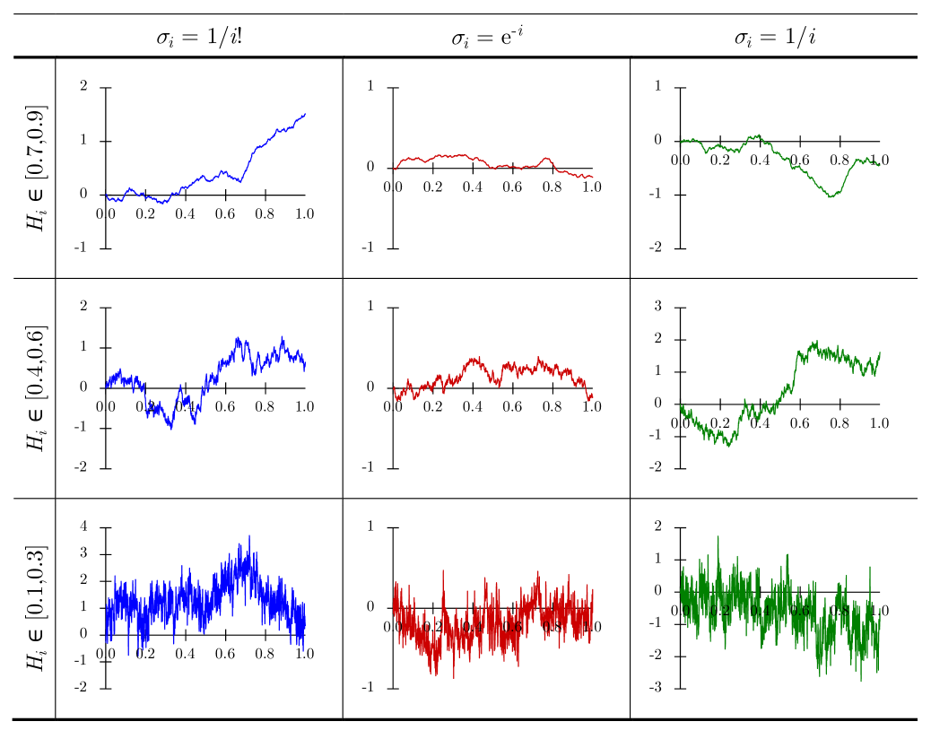
Figure 1. Sample paths of mmfBm with equidistant time points and equidistant Hurst parameters.

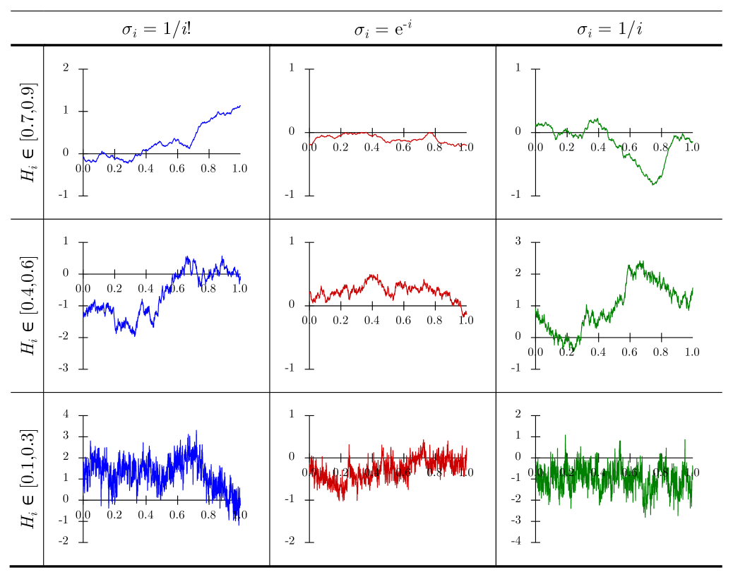
Figure 2. Sample paths of mmfOU with equidistant time points and equidistant Hurst parameters.

References

- [1] E. Azmoodeh, T. Sottinen, L. Viitasaari, and A. Yazigi, Necessary and sufficient conditions for Hölder continuity of Gaussian processes, Statist. Probab. Lett., 94 (2014), pp. 230–235.
- [2] L. A. Barboza and F. G. Viens, Parameter estimation of Gaussian stationary processes using the generalized method of moments, Electron. J. Stat., 11 (2017), pp. 401–439.
- [3] C. Bender, T. Sottinen, and E. Valkeila, Arbitrage with fractional Brownian motion?, Theory Stoch. Process., 13 (2007), pp. 23–34.
- [4] , Pricing by hedging and no-arbitrage beyond semimartingales, Finance Stoch., 12 (2008), pp. 441–468.
- [5] F. Biagini, Y. Hu, B. Øksendal, and T. Zhang, Stochastic calculus for fractional Brownian motion and applications, Probability and its Applications (New York), Springer-Verlag London, Ltd., London, 2008.
- [6] P. Cheridito, Mixed fractional Brownian motion, Bernoulli, 7 (2001), pp. 913–934.
- [7] P. Cheridito, H. Kawaguchi, and M. Maejima, Fractional Ornstein-Uhlenbeck processes, Electron. J. Probab., 8 (2003), pp. no. 3, 14 pp. (electronic).
- [8] R. M. Dudley and R. Norvaiša, An introduction to p-variation and Young integrals: With emphasis on sample functions of stochastic processes, Centre for Mathematical Physics and Stochastics, University of Aarhus, 1998.
- [9] R. M. Dudley and R. Norvaiša, Differentiability of six operators on nonsmooth functions and -variation, vol. 1703 of Lecture Notes in Mathematics, Springer-Verlag, Berlin, 1999. With the collaboration of Jinghua Qian.
- [10] D. Gasbarra, T. Sottinen, and H. Van Zanten, Conditional full support of gaussian processes with stationary increments, Journal of Applied Probability, 48 (2011), pp. 561–568.
- [11] I. Gelfand and G. Shilov, Generalized functions vol 1 (new york: Academic), (1964).
- [12] C. Houdré and J. Villa, An example of infinite dimensional quasi-helix, in Stochastic models (Mexico City, 2002), vol. 336 of Contemp. Math., Amer. Math. Soc., Providence, RI, 2003, pp. 195–201.
- [13] Y. Hu and D. Nualart, Parameter estimation for fractional ornstein–uhlenbeck processes, Statistics & probability letters, 80 (2010), pp. 1030–1038.
- [14] J. Kalemkerian and A. Sosa, Long-range dependence in the volatility of returns in uruguayan sovereign debt indices, Journal of Dynamics & Games, 7 (2020), p. 225.
- [15] A. N. Kolmogoroff, Wienersche Spiralen und einige andere interessante Kurven im Hilbertschen Raum, C. R. (Doklady) Acad. Sci. URSS (N.S.), 26 (1940), pp. 115–118.
- [16] J. Lévy-Véhel, Fractal approaches in signal processing, vol. 3, 1995, pp. 755–775. Symposium in Honor of Benoit Mandelbrot (Curaçao, 1995).
- [17] H. Maleki Almani, S. M. Hosseini, and M. Tahmasebi, Fractional Brownian motion with two-variable Hurst exponent, J. Comput. Appl. Math., 388 (2021), pp. Paper No. 113262, 23.
- [18] B. B. Mandelbrot and J. W. Van Ness, Fractional Brownian motions, fractional noises and applications, SIAM Rev., 10 (1968), pp. 422–437.
- [19] Y. S. Mishura, Stochastic calculus for fractional Brownian motion and related processes, vol. 1929 of Lecture Notes in Mathematics, Springer-Verlag, Berlin, 2008.
- [20] E. Perrin, R. Harba, C. Berzin-Joseph, I. Iribarren, and A. Bonami, nth-order fractional brownian motion and fractional gaussian noises, IEEE Transactions on Signal Processing, 49 (2001), pp. 1049–1059.
- [21] E. Perrin, R. Harba, I. Iribarren, and R. Jennane, Piecewise fractional Brownian motion, IEEE Trans. Signal Process., 53 (2005), pp. 1211–1215.
- [22] G. Samorodnitsky and M. Taqqu, Stable Non-Gaussian Random Processes: Stochastic Models with Infinite Variance, Stochastic Modeling Series, Taylor & Francis, 1994.
- [23] T. P. Sottinen, Fractional Brownian motion in finance and queueing, 2003. Thesis (Ph.D.)–Helsingin Yliopisto (Finland).