Wave Front Sets of Nilpotent Lie Group Representations

Abstract.

Let $G$ be a nilpotent, connected, simply connected Lie group with Lie algebra $\mathfrak{g}$, and $\pi$ a unitary representation of $G$. In this article we prove that the wave front set of $\pi$ coincides with the asymptotic cone of the orbital support of $\pi$, i.e. $\mathrm{WF}(\pi)=\mathrm{AC}(\bigcup_{\sigma\in\mathrm{supp}(\pi)}\mathcal{O}_{\sigma})$, where $\mathcal{O}_{\sigma}\subset i\mathfrak{g}^{\ast}$ is the coadjoint Kirillov orbit associated to the irreducible unitary representation $\sigma\in\hat{G}$.

1. Introduction

The concept of wave front sets was introduced by Sato and Hörmander. Given a distribution $u\in\mathcal{D}^{\prime}(M)$ its wave front set is a closed conical subset $\operatorname{WF}(u)\subset T^{*}M$ that encodes the singularities of the distributions $u$. Informally speaking one can consider the wave front set as those directions in which the distribution is not smooth (in a $C^{\infty}$ sense). Wave front sets are extensively used in PDE theory as a very concise measure of singularities. For example Hörmanders famous theorem about propagation of singularities is formulated in terms of wave front sets.

The concept of the wave front set for a unitary Lie group representation was introduced by Howe [How81]. Given a Lie group $G$ with Lie algebra $\mathfrak{g}$ and a unitary representation $(\pi,\mathcal{H})$ the wave front set of the representation yields a closed $\operatorname{Ad}^{*}(G)$-invariant cone $\operatorname{WF}(\pi)\subset i\mathfrak{g}^{*}$. Informally speaking it captures the singular directions of all matrix coefficients of $\pi$ (see Definition 2.2 for a precise definition). The remarkable property of $\operatorname{WF}(\pi)$ is that it is defined entirely in terms of singularities of matrix coefficients but it captures essential information of the spectral measure of $\pi$. This relation can be expressed by certain wave front-orbital support (WFOS) theorems which we want to explain next: Suppose that the Lie group $G$ is of type I such that we can write any unitary representation $(\pi,\mathcal{H})$ as a direct integral $\pi=\int^{\oplus}_{\hat{G}}\sigma^{m(\sigma)}\mu_{\pi}(\sigma)$ where $\hat{G}$ is the unitary dual endowed with the Fell topology and $\mu_{\pi}$ a Borel measure on $\hat{G}$, the spectral measure of $\pi$. Suppose furthermore that there is a canonical way to associate to any $\sigma\in\operatorname{supp}\mu_{\pi}\subset\hat{G}$ a coadjoint orbit $\mathcal{O}_{\sigma}\subset i\mathfrak{g}^{*}$ (or possibly a finite collection of such orbits), then we define the orbital support to be

(1) $$\mathcal{O}-\operatorname{supp}(\pi):=\bigcup_{\sigma\in\operatorname{supp}(\mu_{\pi})}\mathcal{O}_{\sigma}\subset i\mathfrak{g}^{*}.$$

Furthermore, we define for any subset $S\subset i\mathfrak{g}^{*}$ its asymptotic cone

$$\operatorname{AC}(S):=\{\xi\in i\mathfrak{g}^{*}|\mathcal{C}\text{ an open cone containing }\xi\Rightarrow S\cap\mathcal{C}\text{ unbounded }\}\cup\{0\}.$$

A Wave front-orbital support theorem is then a theorem that states (for a suitable class of Lie groups $G$ and unitary representations $(\pi,\mathcal{H})$) the equality

(2) $$\operatorname{WF}(\pi)=\operatorname{AC}(\mathcal{O}-\operatorname{supp}(\pi))$$

and thus connects the wave front set to the asymptotic support of the spectral measure. For abelian Lie groups the WFOS-theorem is just a reflection of the defintion of the wave front set and Fourier inversion formulas as had been noted by Howe [How81]. For non-commutativ Lie groups the relation is much more subtle and has been shown for compact groups by Kashiwara-Vergne [KV79] and Howe [How81]. Much more recently Harris, He and Ólafson [HHÓ16, Theorem 1.2] have shown a WFOS-theorem for real reductive algebraic groups $G$ and unitary representations $\pi$ which are weakly contained in the tempered representations (see [Har18, HO17] for follow up works that aim to weaken the temperedness assumption).

The practical purpose of WFOS-theorems is that they connect the spectral measure $\mu_{\pi}$ of general unitary representations to the wave front set of $\pi$. While the former is in general very difficult to determine, the latter has been shown to be explicitly calculable in very general settings. For example if $G$ is an arbitrary Lie group and $H\subset G$ a closed subgroup such that $G/H$ carries a non-vanishing $G$-invariant smooth density then one can consider the regular representation of $G$ on $L^{2}(G/H)$. While determining the exact spectral measure (i.e. the Plancherel measure) of $L^{2}(G/H)$ is in general extremely difficult and so far only known for certain classes of homogeneous spaces, the wave front set of $L^{2}(G/H)$ is known [HW17, Theorem 2.1] without any further assumptions

$$\operatorname{WF}(L^{2}(G/H))=\overline{\operatorname{Ad}^{*}(G)i(\mathfrak{g}/\mathfrak{h})^{*}}.$$

Similar identities have also been derived for certain classes of induced representations [HW17, Theorem 2.2 and 2.3] and also the behaviour of wave front sets under restrictions is rather well understood [How81, Prop 1.5][HHÓ16, Corollary 1.4]. Combining the explicit knowledge of $\operatorname{WF}(L^{2}(G/H))$ with a WFOS-theorem one can then deduce results about the Plancherel measures, e.g. existence of discrete series (see e.g. [HW17, Example 7.5][DKKS18, Theorem 21.1]).

In contrast to the knowledge about $\operatorname{WF}(L^{2}(G/H))$ that is known without any structural assumptions on $G$ and only mild assumptions on the quotient $G/H$, the cases in which WFOS-theorems are established are rather limited (abelian [How81], compact [How81, KV79] and real reductive groups [HHÓ16] as mentioned above). One might hope that they can be proven for any class of Lie groups where a suitable relation between unitary irreducible representations and coadjoint orbits is established, for example in the setting of real linear algebraic group (see e.g. [Duf10]). The purpose of this article is to establish a WFOS-theorem for nilpotent Lie groups. We prove

Theorem 1.

Let $G$ be a nilpotent, connected, simply connected Lie group and $\pi$ a unitary representation of $G$. Then

$$\operatorname{WF}(\pi)=\operatorname{AC}(\mathcal{O}-\operatorname{supp}\pi).$$

Where the orbit support (1) is defined by the Kirrilov orbits $\mathcal{O}_{\sigma}\subset i\mathfrak{g}^{*}$ of the unitary irreducible representation $\sigma$.

It was rather surprising to us, that the proof strategy of [HHÓ16] could not be transferred to the setting of nilpotent Lie groups. A central object in the proof of the Wave front-Plancherel theorem in [HHÓ16] was the analysis of integrated characters $\int_{\hat{G}}\chi_{\sigma}f(\sigma)d\mu_{\pi}(\sigma)\in\mathcal{D}^{\prime}(G)$ where $\chi_{\sigma}\in\mathcal{D}^{\prime}(G)$ is the distributional character of the tempered irreducible representation $\sigma$. Harris, He and Ólaffson then use character formulas of Duflo and Rossmann as well as Harish-Chandra’s invariant integrals to relate the wave front set of the integrated characters to the asymptotic orbital support. While Kirillov’s character formula provides a natural (and even simpler) replacement to the Duflo-Rossmann formula, the analogon to the Harish-Chandra invariant integrals for nilpotent groups produces additional singularities which make the proof break down (see [Bud21, Section 5.1] for a detailed discussion of the occurring problems). We therefore had to establish an alternative method to prove the above result. Instead of working with integrated characters and character formulas we directly work with matrix coefficients. In contrast to the characters, the Fourier transform of individual matrix coefficients of an irreducible representation are not supported on the coadjoint orbits. However we can show (Proposition 3.1 and Proposition 3.4) that they are microlocally supported “near” the orbit and that the precise meaning of “near” can be made uniform about all unitary representations. Our proof of these key propositions is based on concrete microlocal estimates on induced representations. The induction scheme hereby is similar to the induction in the traditional proof of Kirillov’s character formula.

Let us briefly outline the article: We first introduce the relevant notion on wave front sets (Section 2.1) and the structure of nilpotent Lie groups and their unitary representations (Section 2.2). We then proof Theorem 1 by proving separately the two inclusions $\operatorname{AC}(\mathcal{O}-\operatorname{supp}(\pi))\subset\operatorname{WF}(\pi)$ (Section 3.1) and $\operatorname{AC}(\mathcal{O}-\operatorname{supp}(\pi))\supset\operatorname{WF}(\pi)$ (Section 3.2). For both inclusions we prove a uniform estimate on the Fourier transforms of individual matrix coefficients (Proposition 3.1 and Proposition 3.4, respectively). A sketch of the central ideas of their proof is given after the statement of each of the two propositions.

Acknowledgements We thank Benjamin Harris, Joachim Hilgert, Jan Frahm and Clemens Weiske for many encouraging discussions and helpful remarks and suggestions. This project has received funding from Deutsche Forschungsgemeinschaft (DFG) (Grant No. WE 6173/1-1 Emmy Noether group “Microlocal Methods for Hyperbolic Dynamics”)

2. Preliminaries

2.1. Wave Front Sets

In this section we give definitions of the wave front set of a distribution and of a unitary Lie group representation and provide some facts about these objects that we will use later in the article.

Let $W$ be a real, finite-dimensional vector space and fix a Lebesgue measure $dx$ on $W$. We define the Fourier transform as the map $\mathcal{F}:\mathcal{S}(W)\to\mathcal{S}(iW^{\ast})$ between Schwartz spaces with

$$\mathcal{F}(\varphi)(\zeta):=\int_{W}\varphi(x)e^{-2\pi\langle\xi,x\rangle}\leavevmode\nobreak\ dx,\quad\xi\in iW^{\ast},$$

and for a tempered distribution $u\in\mathcal{S}^{\prime}(W)$ as $\mathcal{F}(u)\in\mathcal{S}^{\prime}(iW^{\ast})$ with $\mathcal{F}(u)(\psi):=u(\mathcal{F}(\psi))$ for $\psi\in\mathcal{S}(iW^{\ast})$. The inversion formula for $\mathcal{F}:\mathcal{S}(W)\to\mathcal{S}(iW^{\ast})$ gives us

$$\mathcal{F}^{-1}:\mathcal{S}(iW^{\ast})\to\mathcal{S}(W),\quad\psi\mapsto\left(x\mapsto\int_{iW^{\ast}}\psi(\xi)e^{2\pi\langle\xi,x\rangle}\leavevmode\nobreak\ d\xi\right)$$

for a suitable measure $d\xi$ on $iW^{\ast}$.

In addition to that, we define the Fourier transform of a distribution $v\in\mathcal{E}^{\prime}(W)$ with compact support to be

$$\mathcal{F}(v)(\xi):=v\left[e^{-2\pi\langle\xi,\bullet\rangle}\right],\quad\xi\in iW^{\ast}.$$

Definition 2.1.

Let $W$ be a real, finite-dimensional vector space and $u\in\mathcal{D}^{\prime}(X)$ a distribution on an open subset $X\subset W$. Then we say $(x_{0},\xi_{0})\in X\times iW^{\ast}\setminus\{0\}\subset iT^{\ast}X$ is not in the wave front set $\operatorname{WF}(u)\subset iT^{\ast}X$ if there exist open neighborhoods $U$ of $x_{0}$ and $V$ of $\xi_{0}$ and a smooth compactly supported function $\phi\in C_{c}^{\infty}(U)$ with $\phi(x_{0})\neq 0$ such that for all $N\in\mathbb{N}$ there exists a constant $C_{N,\phi}>0$ such that

$$|\mathcal{F}(\phi u)(\tau\xi)|\leq C_{N,\phi}|\tau|^{-N}\quad\forall\,\tau\gg 0,\xi\in V.$$

Note that $(x,0)\in iT^{\ast}X$ is never in the wave front set (contrary to Definition 2.2 for unitary representations) because in order to analyze the singularities of a function or distribution it only makes sense to look in the directions $\xi\neq 0$.
Furthermore, it is easily seen from the definition that the wave front set $\operatorname{WF}(u)\subset iT^{\ast}X$ is a closed cone (in the second component).

Now, if $\psi:X\to Y$ is a diffeomorphism between two open sets and $u$ is a distribution on $Y$, then $\psi^{\ast}\operatorname{WF}(u)=\operatorname{WF}(\psi^{\ast}u)$, where the pullback on the cotangent bundle is defined by

$$\psi^{\ast}(y,\xi)=\left(\psi^{-1}(y),(D\psi(\psi^{-1}(y)))^{T}\xi\right),\quad(y,\xi)\in iT^{\ast}Y.$$

Thus, the notion of the wave front set of a distribution on a smooth manifold is independent of the choice of local coordinates and is therefore well-defined.

Now let $G$ be a $n$-dimensional Lie group with Lie algebra $\mathfrak{g}$ and $(\pi,\mathcal{H})$ a unitary representation of $G$. Denote by $J_{1}(\mathcal{H})$ the space of trace class operators with trace class norm $\|T\|_{1}$.

Definition 2.2.

The wave front set of a unitary representation $\pi$ is defined as the closure of the union of the wave front sets at the identity of the matrix coefficients of $\pi$:

$$\operatorname{WF}(\pi):=\overline{\bigcup_{v,w\in\mathcal{H}}\operatorname{WF}_{e}(\langle\pi(g)v,w\rangle_{\mathcal{H}})}\cup\{0\}\subset iT^{\ast}_{e}G\cong i\mathfrak{g}^{\ast}.$$

Here we use the convention that zero is always in the wave front set (contrary to Definition 2.1) because it makes the statements of the results for unitary representations cleaner.
Howe used in [How81] the equivalent definition

$$\operatorname{WF}(\pi)=\overline{\bigcup_{T\in J_{1}(\mathcal{H})}\operatorname{WF}_{e}(\operatorname{Tr}_{\pi}(T))}\cup\{0\},$$

where $\operatorname{Tr}_{\pi}(T):=\operatorname{Tr}(\pi(\cdot)T)$, $T\in J_{1}(\mathcal{H})$, is a continuous bounded function on $G$ regarded as a distribution on $G$ by integration. The equivalence of these definitions was shown in [HHÓ16, Proposition 2.4].

It is a well-known fact that the wave front set $\operatorname{WF}(\pi)\subset i\mathfrak{g}^{\ast}$ is a closed, $\operatorname{Ad}^{\ast}(G)$-invariant cone.

The following result provides another description of the wave front set which we will use in our proof.

Lemma 2.3 (see [How81, Theorem 1.4 v)] and [HHÓ16, Lemma 2.5 (iii)]).

Let $\xi_{0}\in i\mathfrak{g}^{\ast}$. Then $\xi_{0}\notin\operatorname{WF}(\pi)$ if and only if there is an open set $e\in U\subset G$ on which the logarithm is a well-defined diffeomorphism onto its image and an open set $\xi_{0}\in V\subset i\mathfrak{g}^{\ast}$ such that for every $\phi\in C_{c}^{\infty}(U)$ there exists a family of constants $C_{N}(\phi)>0$ independent of both $\xi\in V$ and $T\in J_{1}(H)$, such that

$$\left|\int_{G}\operatorname{Tr}_{\pi}(T)(g)e^{-2\pi\tau\xi(\log g)}\phi(g)\leavevmode\nobreak\ dg\right|\leq C_{N}(\phi)\|T\|_{1}\tau^{-N}$$

for $\tau\gg 0$, $\xi\in V$, $T\in J_{1}(H)$.

For our proof in Section 3.1 we need to know more about the dependence of the constant $C_{N}(\phi)$ on the cut-off function $\phi\in C_{c}^{\infty}(G)$.

Lemma 2.4.

For all $N>n=\dim(G)$ the above statement holds with the choice of the constant $C_{N}(\phi)=C_{N}\|\phi\|_{W^{N+n,1}}$ where $\|\phi\|_{W^{M,1}}:=\sum_{|\alpha|\leq M}\|D^{\alpha}\phi\|_{L^{1}}$ is a Sobolev norm.

Proof.

We may assume without loss of generality that in Lemma 2.3 $V=B_{2\epsilon}(\xi_{0})$ for an $\frac{1}{2}>\varepsilon>0$ and $\|\xi_{0}\|=1$, and may prove our statement for $\xi\in V^{\prime}\coloneq B_{\epsilon}(\xi_{0})$ with $\|\xi\|=1$. Now, let $U\subset G$ be the open set given by Lemma 2.3 and take $U^{\prime}\subsetneqq U$ open and $\chi\in C_{c}^{\infty}(\log(U))$ a function on $\mathfrak{g}$ with $\chi=1$ on $\log(U^{\prime})\subset\mathfrak{g}$. Then we can estimate for all $\phi\in C_{c}^{\infty}(U^{\prime})$, $\varphi=\phi\circ\exp\in C_{c}^{\infty}(\mathfrak{g})$:

$$I(\phi,\xi,T)(\tau) :=\int_{G}\operatorname{Tr}_{\pi}(T)(g)e^{-2\pi\tau\xi(\log g)}\phi(g)\leavevmode\nobreak\ dg=\int_{\mathfrak{g}}\operatorname{Tr}_{\pi}(T)(\exp(X))e^{-2\pi\tau\xi(X)}\chi(X)\varphi(X)\leavevmode\nobreak\ dg$$

$$=\int_{i\mathfrak{g}^{\ast}}\left(\int_{\mathfrak{g}}\operatorname{Tr}_{\pi}(T)(\exp(X))\chi(X)e^{-2\pi\eta(X)}dX\right)\left(\int_{\mathfrak{g}}\varphi(Y)e^{2\pi(\eta-\tau\xi)(Y)}dY\right)d\eta,$$

and define $J_{1}(\eta)\coloneq\int_{\mathfrak{g}}\operatorname{Tr}_{\pi}(T)(\exp(X))\chi(X)e^{-2\pi\eta(X)}dX$ and $J_{2}(\eta)\coloneq\int_{\mathfrak{g}}\varphi(Y)e^{2\pi(\eta-\tau\xi)(Y)}dY$. With the $\frac{1}{2}>\varepsilon>0$ chosen above we split up the integral as $I(\phi,\xi,T)(\tau)=I_{1}+I_{2}$ where

$$I_{1}\coloneq\int_{\|\tau\xi-\eta\|\geq\varepsilon\tau}J_{1}(\eta)J_{2}(\eta)d\eta,\quad I_{2}\coloneq\int_{B_{\varepsilon\tau}(\tau\xi)}J_{1}(\eta)J_{2}(\eta)d\eta.$$

For the first integral we estimate for $\eta\notin B_{\varepsilon\tau}(\tau\xi)$ by estimation of the integrand and partial integration, respectively

$$|J_{1}(\eta)|\leq\|T\|_{1}\|\chi\|_{L^{1}},\quad|J_{2}(\eta)|\leq\|\varphi\|_{W^{N,1}}\|\tau\xi-\eta\|^{-N}$$

and therefore

$$|I_{1}| \leq\|T\|_{1}\|\chi\|_{L^{1}}\|\varphi\|_{W^{N,1}}\int_{\|\tau\xi-\eta\|\geq\varepsilon\tau}\|\tau\xi-\eta\|^{-N}d\eta=\|T\|_{1}\|\chi\|_{L^{1}}\|\varphi\|_{W^{N,1}}\int_{\varepsilon\tau}^{\infty}r^{-N}r^{n-1}dr$$

$$=\|T\|_{1}\|\chi\|_{L^{1}}\|\varphi\|_{W^{N,1}}\varepsilon^{-N+n}\tau^{-N+n}.$$

For the second integral we estimate for $\eta\in B_{\varepsilon\tau}(\tau\xi)$ with Lemma 2.3 applied to $\chi$ and $\frac{1}{\|\eta\|}\eta\in B_{2\epsilon}(\xi_{0})=V$

$$|J_{1}(\eta)|\leq\|T\|_{1}C_{N}(\chi)\|\eta\|^{-N},\quad|J_{2}(\eta)|\leq\|\varphi\|_{L^{1}}\leq\|\varphi\|_{W^{N,1}}.$$

Since $\|\eta\|\geq(1-2\varepsilon)\tau$ we have

$$|I_{2}| \leq\|T\|_{1}C_{N}(\chi)\|\varphi\|_{W^{N,1}}\int_{B_{\varepsilon\tau}(\tau\xi)}\|\eta\|^{-N}d\eta$$

$$\leq\|T\|_{1}C_{N}(\chi)\|\varphi\|_{W^{N,1}}((1-2\varepsilon)\tau)^{-N}C(\varepsilon\tau)^{n}\leq C_{N}\|T\|_{1}\|\varphi\|_{W^{N,1}}\tau^{-N+n}.$$

This proves the statement with $U^{\prime}$ as the open neighborhood of $e\in G$ and $V^{\prime}$ as the open neighborhood of $\xi_{0}$ in $i\mathfrak{g}^{\ast}$. ∎

Lastly, the following simple result gives us an idea why wave front sets might be interesting for the decomposition of unitary representations.

Proposition 2.5.

Let $(\pi_{1},\mathcal{H}_{1})$,…, $(\pi_{k},\mathcal{H}_{k})$ be unitary representations of $G$, then

$$\operatorname{WF}\left(\bigoplus_{j=1}^{k}\pi_{j}\right)=\bigcup_{j=1}^{k}\operatorname{WF}(\pi_{j}).$$

2.2. Nilpotent Lie Groups

In order to prove Theorem 1 we use the structure theory of nilpotent Lie algebras and Lie groups. The required results below are mostly from the book by Corwin and Greenleaf [CG90].

Let $G$ be a nilpotent, connected, simply connected Lie group with Lie algebra $\mathfrak{g}$ of dimension $n$ and $\mathfrak{g}^{\ast}$ its vector space dual. By $\hat{G}$ we denote the unitary dual of $G$ and by $i\mathfrak{g}^{\ast}/G$ the space of coadjoint orbits.

The main results are the following two theorems:

Theorem 2 (see [CG90, Theorems 2.2.1 - 2.2.4]).

There exists a homeomorphism $\hat{G}\to i\mathfrak{g}^{\ast}/G$, $\sigma\mapsto\mathcal{O}_{\sigma}$, and $\sigma_{l}\leftmapsto\mathcal{O}_{l}=\operatorname{Ad}^{\ast}(G)l$. For the continuity of the map $i\mathfrak{g}^{\ast}/G\to\hat{G}$ see [Kir62, Theorem 8.2] and for the continuity of the map $\hat{G}\to i\mathfrak{g}^{\ast}/G$ see [Bro73].

The structure and parametrization of the coadjoint orbits is given by

Theorem 3 (see [CG90, Theorem 3.1.14]).

Fix a (strong Malcev) basis $\{X_{1},\ldots,X_{n}\}$ of $\mathfrak{g}$. Then there exits a finite set $D$ of orbit types. Denote by $U_{d}\subset i\mathfrak{g}^{\ast}$ the union of all orbits of type $d\in D$. Moreover, all orbits in $U_{d}$ have the same dimension $d_{n}$.
For each $d\in D$ there also exists a cross-section $\Sigma_{d}\subset i\mathfrak{g}^{\ast}$ of the orbits in $U_{d}$, i.e. each orbit $\mathcal{O}\subset U_{d}$ intersects $\Sigma_{d}$ in a unique point. Then

$$\Sigma:=\bigsqcup_{d\in D}\Sigma_{d}\cong i\mathfrak{g}^{\ast}/G$$

is a cross-section of all $\operatorname{Ad}^{\ast}(G)$-orbits.
Furthermore, for each $d\in D$ there exists a decomposition

$$i\mathfrak{g}^{\ast}=V_{S(d)}\oplus V_{T(d)}$$

as a direct sum of vector spaces and a birational, non-singular, surjective map

$$\psi_{d}\colon\Sigma_{d}\times V_{S(d)}\rightarrow U_{d}$$

such that for each $l\in\Sigma_{d}$ its orbit is given by $\mathcal{O}_{l}=\psi_{d}\left(l,V_{S(d)}\right)$.

Remark 2.6.

For $d\in D$ we know $\mathcal{H}_{l}\cong L^{2}\left(\mathbb{R}^{d_{n}/2}\right)$ for all $l\in\Sigma_{d}$, where $d_{n}=\dim\mathcal{O}_{l}$ for all $l\in\Sigma_{d}$.

Now, we collect the ingredients and underlying concepts of the main statements starting at the level of nilpotent Lie algebras. These details will not only be presented as background material but will be crucial for our own results.

Lemma 2.7 (see [CG90, Kirillov’s Lemma 1.1.12]).

Let $\mathfrak{g}$ be a non-abelian nilpotent Lie algebra whose center $\mathfrak{z}(\mathfrak{g})=\mathbb{R}Z$ is one-dimensional. Then $\mathfrak{g}$ can be written as

$$\mathfrak{g}=\mathbb{R}Z\oplus\mathbb{R}Y\oplus\mathbb{R}X\oplus\mathfrak{w}=\mathbb{R}X\oplus\mathfrak{g}_{0},$$

a vector space direct sum with a suitable subspace $\mathfrak{w}$. Furthermore, $[X,Y]=Z$ and $\mathfrak{g}_{0}=\mathbb{R}Y\oplus\mathbb{R}Z\oplus\mathfrak{w}$ is the centralizer of $Y$ and an ideal.

In order to study the coadjoint orbits we start with

Lemma 2.8 (see [CG90, Lemma 1.3.2]).

For $l\in i\mathfrak{g}^{\ast}$ we define the bilinear form $B_{l}(X,Y)=l([X,Y])$ on $\mathfrak{g}$. Then the radical

(3) $$\mathfrak{r}_{l}:=\{X\in\mathfrak{g}:B_{l}(X,Y)=0\;\forall\;Y\in\mathfrak{g}\}=\{X\in\mathfrak{g}:\operatorname{ad}^{\ast}(X)l=0\}$$

has even codimension in $\mathfrak{g}$. Hence coadjoint orbits are of even dimension.
They are actually symplectic manifolds with the non-degenerate skew symmetric 2-form $\omega(l^{\prime})\in\Lambda^{2}(T_{l^{\prime}}\mathcal{O}_{l})$ such that $\omega(l^{\prime})(-(\operatorname{ad}^{\ast}X)l^{\prime},-(\operatorname{ad}^{\ast}Y)l^{\prime})=l^{\prime}([X,Y])$, $l^{\prime}\in\mathcal{O}_{l}$. Note that $\omega$ is $\operatorname{Ad}^{\ast}(G)$-invariant.

Now, we are interested in how we can define an irreducible unitary representation of $G$ given an element $l\in i\mathfrak{g}^{\ast}$ (with Theorem 2 in mind).

Definition 2.9.

A polarizing subalgebra for $l\in i\mathfrak{g}^{\ast}$ is a subalgebra $\mathfrak{m}\subset\mathfrak{g}$ that is a maximal isotropic subspace for the bilinear form $B_{l}:\mathfrak{g}\times\mathfrak{g}\to i\mathbb{R}$.
They are also called maximal subordinate subalgebras for $l$.

Proposition 2.10 (see [CG90, Proposition 1.3.3]).

Let $\mathfrak{g}$ be a nilpotent Lie algebra and let $l\in i\mathfrak{g}^{\ast}$. Then there exists a polarizing subalgebra for $l$.

Now, for $l\in i\mathfrak{g}^{\ast}$ choose a polarizing $\mathfrak{m}$ and let $M=\exp\mathfrak{m}$. Then $\chi_{l}(\exp Y)=e^{2\pi l(Y)}$ is a one-dimensional representation of $M$ since $l([\mathfrak{m},\mathfrak{m}])=0$. Hence, we can define

$$\sigma_{l}:=\operatorname{Ind}_{M}^{G}(\chi_{l}).$$

More precisely,

$$\mathcal{H}_{l}=\{f:G\to\mathbb{C}\text{ measurable}:f(mg)=\chi_{l}(m)f(g)\;\forall m\in M\text{ and }\int\limits_{M\backslash G}\|f(g)\|^{2}d\dot{g}<\infty\}$$

and

$$(\sigma_{l}(x)f)(g)=f(gx)\quad\forall\;x\in G,f\in\mathcal{H}_{l}.$$

With this construction one can prove the bijection $\hat{G}\cong i\mathfrak{g}^{\ast}/G$.

The proof is by induction on the dimension of $G$. The inductive step is based an the following statement.

Proposition 2.11 (see [CG90, Proposition 1.3.4]).

Let $\mathfrak{g}_{0}$ be a subalgebra of codimension 1 in a nilpotent Lie algebra $\mathfrak{g}$, let $l\in i\mathfrak{g}^{\ast}$, and let $l_{0}=l\big{|}_{\mathfrak{g}_{0}}$. Let $\mathfrak{r}_{l}$ be the radical defined in Equation (3). Then there are two mutually exclusive possibilities:

• Case I characterized by any of the following equivalent properties:

  1. $\mathfrak{r}_{l}\nsubseteq\mathfrak{g}_{0}$;

  2. $\mathfrak{r}_{l}\supset\mathfrak{r}_{l_{0}}$;

  3. $\mathfrak{r}_{l_{0}}$ of codimension 1 in $\mathfrak{r}_{l}$.

  In this case, if $\mathfrak{m}$ is a polarizing subalgebra for $l$, then $\mathfrak{m}_{0}=\mathfrak{m}\cap\mathfrak{g}_{0}$ is a polarizing subalgebra for $l_{0}$; $\mathfrak{m}_{0}$ is of codimension 1 in $\mathfrak{m}$ and $\mathfrak{m}=\mathfrak{r}_{l}+\mathfrak{m}_{0}$.

• Case II characterized by any of the following equivalent properties:

  1. $\mathfrak{r}_{l}\subset\mathfrak{g}_{0}$;

  2. $\mathfrak{r}_{l}\subset\mathfrak{r}_{l_{0}}$;

  3. $\mathfrak{r}_{l}$ of codimension 1 in $\mathfrak{r}_{l_{0}}$.

  In this case, any polarizing subalgebra for $l_{0}$ is also polarizing for $l$.

Even though this is a rather technical result its significance becomes clearer in the next statements since we also know how the irreducible representations and the orbits of $G$ and $G_{0}$ are connected in these two cases.

Theorem 4 (see [CG90, Theorem 2.5.1]).

Let the notation be as above. Let $p:i\mathfrak{g}^{\ast}\to i\mathfrak{g}_{0}^{\ast}$ be the canonical projection and $G_{0}=\exp(\mathfrak{g}_{0})$.

1. In Case I, where $\mathfrak{r}_{l}\nsubseteq\mathfrak{g}_{0}$, we have

   $$\sigma_{l_{0}}\cong\sigma_{l}\big{|}_{G_{0}}\quad\text{and}\quad p:\mathcal{O}_{l}\to\mathcal{O}_{l_{0}}:=\operatorname{Ad}^{\ast}(G_{0})l_{0}\text{ is a bijection}$$

   (see Figure 1).

2. In Case II, where $\mathfrak{r}_{l}\subset\mathfrak{g}_{0}$, we have

   $$\sigma_{l}\cong\operatorname{Ind}_{G_{0}}^{G}(\sigma_{l_{0}}),\quad p(\mathcal{O}_{l})=\bigsqcup_{t\in\mathbb{R}}(\operatorname{Ad}^{\ast}\exp tX)\mathcal{O}_{l_{0}}\quad\text{and}\quad\mathcal{O}_{l}=p^{-1}(p(\mathcal{O}_{l})),$$

   where $X$ is any element such that $\mathfrak{g}=\mathbb{R}X\oplus\mathfrak{g}_{0}$.

Figure 1. Orbits of $G_{0}$ and $G$ in Case II of Theorem 4

In order to nicely formulate the statements about the estimate of matrix coefficients in Section 3 we introduce the following notation:

Definition 2.12.

Let $N$ be a nilpotent, connected, simply connected, nilpotent Lie group with Lie algebra $\mathfrak{n}$ and fix an inner product on $\mathfrak{n}$. Then for a nilpotent Lie algebra $\mathfrak{g}$ we write $(\mathfrak{g},\langle,\rangle_{\mathfrak{g}})\prec(\mathfrak{n},\langle,\rangle_{\mathfrak{n}})$ if and only if $\mathfrak{g}$ can occur in the induction process of $\mathfrak{n}$ using the two cases of Theorem 4, i.e. can be obtained via passing to a quotient by a central element or taking the subalgebra of co-dimension 1 given by Kirillov’s Lemma 2.7, and the inner product on $\mathfrak{g}$ is the one it inherits from $\mathfrak{n}$.

We end this section with a technical lemma we will use in a proof in the next section regarding the transition maps between two charts of $G$:
Let $X_{0}\in\mathfrak{g}$ with $\|X_{0}\|=1$. Given an inner product in $\mathfrak{g}$ we consider the orthogonal decomposition $\mathfrak{g}=\mathbb{R}X_{0}\oplus V$ as vector spaces and define $\beta_{X_{0}}:\mathbb{R}X_{0}\oplus V\to G,tX_{0}+v\mapsto\exp(tX_{0})\exp(v)$. Then $\beta_{X_{0}}$ is a global chart by an argument analogous to [CG90, Proposition 1.2.8] (after choosing a weak Malcev basis of $\mathfrak{g}$ through $\mathbb{R}X_{0}$ which exits by [CG90, Theorem 1.1.13]). Now, let $\kappa_{X_{0}}=\beta_{X_{0}}^{-1}\circ\exp:\mathfrak{g}\to\mathfrak{g}$ be the smooth transition map. Then for each $N\in\mathbb{N}$ the quantity $C_{\mathfrak{g},N}\coloneq\sup_{\|X_{0}\|=1}\|\kappa_{X_{0}}\|_{C^{N}(B_{R}(0))}$ is finite since it depends continuously on $X_{0}\in S^{n-1}$.

Lemma 2.13.

Let $\mathfrak{h}\subset\mathfrak{g}$ be a subalgebra of co-dimension 1 or $\mathfrak{h}=\mathfrak{g}/\mathbb{R}Z$ a quotient with $Z\in\mathfrak{z}(\mathfrak{g})$ and take compatible inner products on $\mathfrak{g}$ and $\mathfrak{h}$. Then $C_{\mathfrak{h},N}\leq C_{\mathfrak{g},N}$ for all $N\in\mathbb{N}$.

Proof.

We start with the case that $\mathfrak{h}\subset\mathfrak{g}$ is a subalgebra of co-dimension 1. Then the exponential map $\exp^{\mathfrak{h}}$ on $\mathfrak{h}$ is just the exponential map $\exp^{\mathfrak{g}}$ of $\mathfrak{g}$ restricted to $\mathfrak{h}$. In particular, for $X_{0}\in\mathfrak{h}$ with $\|X_{0}\|=1$ we have $\mathfrak{h}=\mathbb{R}X_{0}\oplus V_{\mathfrak{h}}$ and $\mathfrak{g}=\mathbb{R}X_{0}\oplus V_{\mathfrak{h}}\oplus\mathfrak{h}^{\perp}$, $V_{\mathfrak{g}}=V_{\mathfrak{h}}\oplus\mathfrak{h}^{\perp}$. Thus, $\beta_{X_{0}}^{\mathfrak{h}}=\beta_{X_{0}}^{\mathfrak{g}}|_{\mathfrak{h}}$ and therefore $\kappa_{X_{0}}^{\mathfrak{h}}=\kappa_{X_{0}}^{\mathfrak{g}}|_{\mathfrak{h}}$ and $C_{\mathfrak{h},N}\leq C_{\mathfrak{g},N}$.

If $\mathfrak{h}=\mathfrak{g}/\mathbb{R}Z$ is a quotient with $Z\in\mathfrak{z}(\mathfrak{g})$ we consider the orthogonal complement $W\subset\mathfrak{g}$ of $\mathbb{R}Z$ in $\mathfrak{g}$ and the vector space isomorphism $\iota:\mathfrak{h}\to W$ such that $\operatorname{pr}:\mathfrak{g}\to\mathfrak{h}$ corresponds to the orthogonal projection. On the level of the Lie groups we have $H=G/A$ with $A=\exp(\mathbb{R}Z)$, and $\exp^{\mathfrak{h}}(X+\mathbb{R}Z)=\exp^{\mathfrak{g}}(\iota(X))A\in H$, $\log^{\mathfrak{h}}(gA)=\log^{\mathfrak{g}}(g)+\mathbb{R}Z$.
Now, let $\overline{X}_{0}=X_{0}+\mathbb{R}Z\in\mathfrak{h}$, $\|X_{0}\|=1$, and $\mathfrak{h}=\mathbb{R}\overline{X}_{0}\oplus V_{\mathfrak{h}}$. Then $\beta_{\overline{X}_{0}}^{\mathfrak{h}}(t\overline{X}_{0}+\overline{v})=\beta_{\iota(X_{0})}^{\mathfrak{g}}(\iota(tX_{0}+v))A$ since $Z\in\mathfrak{z}(\mathfrak{g})$, and $\kappa_{\overline{X}_{0}}^{\mathfrak{h}}(t\overline{X}_{0}+\overline{v})=\kappa_{\iota(X_{0})}^{\mathfrak{g}}(\iota(tX_{0}+v))+\mathbb{R}Z=\operatorname{pr}_{\mathfrak{h}}\circ\kappa_{\iota(X_{0})}^{\mathfrak{g}}(\iota(tX_{0}+v))$. This finishes the proof since the projection $\operatorname{pr}_{\mathfrak{h}}$ can only reduce the norm of derivatives. ∎

3. Proof of Theorem 1

Let $G$ be a nilpotent, connected, simply connected Lie group with Lie algebra $\mathfrak{g}$ of dimension $n$ and $\mathfrak{g}^{\ast}$ its vector space dual. By $\hat{G}$ we denote the unitary dual. It is isomorphic to the space of coadjoint orbits $i\mathfrak{g}^{\ast}/G$. Let $(\pi,\mathcal{H})$ be a unitary representation of $G$. Then we can write

(4) $$\pi\cong\int_{\hat{G}}^{\oplus}\sigma^{\oplus m(\pi,\sigma)}\leavevmode\nobreak\ d\mu_{\pi}(\sigma),\quad\mathcal{H}\cong\int_{\hat{G}}^{\oplus}\mathcal{H}_{\sigma}^{\oplus m(\pi,\sigma)}\leavevmode\nobreak\ d\mu_{\pi}(\sigma),$$

where $m(\pi,\sigma)$ keeps track of the multiplicity of $\sigma$ in $\pi$. We recall that for such a representation the orbital support of $\pi$ is given by

$$\mathcal{O}-\operatorname{supp}\pi=\bigcup_{\sigma\in\operatorname{supp}(\pi)}\mathcal{O}_{\sigma}\;\subset i\mathfrak{g}^{\ast},\quad\operatorname{supp}(\pi)=\operatorname{supp}(\mu_{\pi}),$$

where $\mathcal{O}_{\sigma}\subset i\mathfrak{g}^{\ast}$ is the orbit of the coadjoint action corresponding to $\sigma\in\hat{G}$ under the isomorphism $\hat{G}\;\cong\;i\mathfrak{g}^{\ast}/G$ (see Theorem 2).
We start by using the structure of nilpotent Lie groups and the unitary representations. By Theorem 3 after fixing a strong Malcev basis of $\mathfrak{g}$ we have

$$\hat{G}\;\cong\;i\mathfrak{g}^{\ast}/G\;\cong\;\Sigma=\bigsqcup_{d\in D}\Sigma_{d}\;\subset i\mathfrak{g}^{\ast},$$

where $\Sigma$ is a cross-section of all $G$-orbits and $\Sigma_{d}$ is a cross-section of all orbits of a certain type $d\in D$, which, in particular, all have the same dimension. Moreover, the set $D$ is finite.
Thus, we can push $\mu_{\pi}$ forward to a positive measure on $\Sigma$ and obtain

$$\pi \cong \int^{\oplus}_{\Sigma}\sigma_{l}^{\oplus m(\pi,\sigma_{l})}\leavevmode\nobreak\ d\mu_{\pi}(l)$$

$$= \bigoplus_{d\in D}\int^{\oplus}_{\Sigma_{d}}\sigma_{l}^{\oplus m(\pi,\sigma_{l})}\leavevmode\nobreak\ d\mu_{\pi}(l)=:\bigoplus_{d\in D}\pi_{d}.$$

With this decomposition we have

$$\operatorname{WF}(\pi)=\bigcup_{d\in D}\operatorname{WF}(\pi_{d}),\qquad\operatorname{AC}(\mathcal{O}-\operatorname{supp}\pi)=\bigcup_{d\in D}\operatorname{AC}(\mathcal{O}-\operatorname{supp}\pi_{d})$$

by Proposition 2.5 and the fact that $\operatorname{AC}\left(\bigcup_{i=1}^{n}S_{i}\right)=\bigcup_{i=1}^{n}\operatorname{AC}(S_{i})$.
Therefore, it suffices to show that

(5) $$\operatorname{AC}(\mathcal{O}-\operatorname{supp}(\pi_{d}))=\operatorname{WF}(\pi_{d})\quad\forall\;d\in D.$$

From now on we fix $d\in D$ and may assume that all the irreducible representations in the support of $\pi$ are of the form $\sigma_{l}$ for an $l\in\Sigma_{d}\subset U_{d}$, where $U_{d}\subset i\mathfrak{g}^{\ast}$ is the set of all $l\in i\mathfrak{g}^{\ast}$ such that its orbit $\mathcal{O}_{l}=\operatorname{Ad}^{\ast}(G)l$ is of type $d$ (see Theorem 3).

Our strategy in the proof of (5) is to prove both inclusions separately in the following two subsections. In both cases we begin with single matrix coefficients $m^{\sigma}_{u,v}(g)=\langle\sigma(g)u,v\rangle$, $\sigma\in\hat{G}$ of type $d$. For the inclusion $\operatorname{AC}(\mathcal{O}-\operatorname{supp}(\pi))\subset\operatorname{WF}(\pi)$ we find vectors $u,v\in\mathcal{H}_{\sigma}$ such that the Fourier transform $\mathcal{F}(m^{\sigma}_{u,v})$ is bounded from below close to the corresponding orbit $\mathcal{O}_{\sigma}$ (see Propositions 3.1 and 3.2 in Subsection 3.1). For the other inclusion $\operatorname{WF}(\pi)\subset\operatorname{AC}(\mathcal{O}-\operatorname{supp}(\pi))$ we show that far away from the orbit $\mathcal{O}_{\sigma}$ the Fourier transform of all matrix coefficients $m^{\sigma}_{u,v}$ is rapidly decaying (see Proposition 3.4 in Subsection 3.2). Since in both statements the constants can be chosen uniformly for all representations $\sigma\in\hat{G}$ we can then use them to show the desired estimates for the matrix coefficient $m^{\pi}_{u,v}(g)=\langle\pi(g)u,v\rangle=\int^{\oplus}_{\Sigma_{d}}m^{\sigma_{l}}_{u_{l},v_{l}}(g)\leavevmode\nobreak\ d\mu_{\pi}(l)$ (with corresponding $u_{l},v_{l}\in\mathcal{H}_{l}^{\oplus m_{l}}$) which imply the relation of $\operatorname{AC}(\mathcal{O}-\operatorname{supp}(\pi))$ and $\operatorname{WF}(\pi)$.

3.1. Proof of the Inclusion $\operatorname{AC}(\mathcal{O}-\operatorname{supp}(\pi))\subset\operatorname{WF}(\pi)$

For the first inclusion we use Lemma 2.4 which states in our setting with $n=\dim\mathfrak{g}$:

$$\xi\notin\operatorname{WF}(\pi)\quad\quad\Leftrightarrow\quad\quad\exists\;e\in U\subset G,\xi\in V\subset i\mathfrak{g}^{\ast}\;\forall\;\phi\in C_{c}^{\infty}(U)\;\forall\;N>n\;\exists\;C_{N}>0:$$

(6) $$|\mathcal{F}(\langle\pi(\bullet)u,v\rangle\phi)(t\eta)|\leq C_{N}\|\phi\|_{W^{N+n,1}}\|u\|\|v\|t^{-N}\quad\text{ for }t\gg 0,\;\eta\in V,\;u,v\in\mathcal{H},$$

where the constants $C_{N}$ may be chosen independent of both $\eta\in V$ and $u,v\in\mathcal{H}$.

As mentioned above we need to find matrix coefficients whose Fourier transform is bounded from below:

Proposition 3.1.

Fix an inner product on $\mathfrak{g}$. There exist $C,\varepsilon>0$ and $1>\delta>0$ such that for all $\zeta\in U_{d}\subset i\mathfrak{g}^{\ast}$ we can find vectors $u_{\zeta}\in\mathcal{H}_{\zeta}^{\infty}$, $v_{\zeta}\in\mathcal{H}_{\zeta}$ with $\|u_{\zeta}\|=\|v_{\zeta}\|=1$ that depend measurably on $\zeta$ (i.e. the resulting map $U_{d}\to L^{2}(\mathbb{R}^{d_{n}/2})\cong\mathcal{H}_{\zeta}$ is measurable) such that for all $\eta\in U_{d}$ with $\|\eta-\zeta\|<\varepsilon^{-1}\delta$ the following estimate holds for all non-negative $\phi\in C_{c}^{\infty}(B_{\varepsilon\langle\|\zeta\|\rangle^{-1/2}}(0))$:

$$\operatorname{Re}\left(\int_{\mathfrak{g}}\langle\sigma_{\zeta}(\exp(X))u_{\zeta},v_{\zeta}\rangle\phi(X)e^{-2\pi\eta(X)}\leavevmode\nobreak\ dX\right)\geq C\cdot\int_{\mathfrak{g}}\phi(X)\leavevmode\nobreak\ dX\geq 0.$$

Before we can begin with the proof however, we will need to restate this proposition in a more detailed version (see Proposition 3.2). This is necessary since we want to prove it by induction over $\dim(\mathfrak{g})$ and need a more detailed induction statement for this. We use the notation introduced in Definition 2.12 to specify the dependencies of the occurring constants. The proof of Proposition 3.2 will be based on the distinction of cases for subalgebras of codimension 1 as in Theorem 4. We therefore distinguish the following cases:

• If $\zeta(Z)=0$ for some nonzero $Z\in\mathfrak{z}(\mathfrak{g})$, we consider $\overline{\mathfrak{g}}=\mathfrak{g}/(\mathbb{R}\cdot Z)$, $\overline{\zeta}=\operatorname{pr}_{i\overline{\mathfrak{g}}^{\ast}}(\zeta)$ and find that $\sigma_{\zeta}|_{\overline{G}}\cong\sigma_{\overline{\zeta}}$ and $\mathcal{H}_{\zeta}\cong\mathcal{H}_{\overline{\zeta}}$ analogously to Case I of Theorem 4. Thus, we can use for $\sigma_{\zeta}$ the same vectors that the induction hypothesis applied to $\sigma_{\overline{\zeta}}$ gives us and check the desired estimates.

• If $\mathfrak{z}(\mathfrak{g})=\mathbb{R}\cdot Z$ and $\zeta(Z)\neq 0$, Kirillov’s Lemma 2.7 gives us a subalgebra $\mathfrak{g}_{0}$ to which we apply the induction hypothesis. Writing $\zeta_{0}=\operatorname{pr}_{i\mathfrak{g}_{0}^{\ast}}(\zeta)$ Theorem  4 tells us that $\sigma_{\zeta}=\operatorname{Ind}_{G_{0}}^{G}(\sigma_{\zeta_{0}})$ and this identification allows us to construct the desired vectors $u_{\zeta},v_{\zeta}\in\mathcal{H}_{\zeta}$ from two vectors $u_{\zeta_{0}},v_{\zeta_{0}}\in cH_{\zeta_{0}}$ that are obtained from the induction hypothesis. However, two difficulties arise: In a first step, we can only construct a distributional vector in $\mathcal{H}_{\zeta}^{-\infty}$ which we then approximate in the next step to find a suitable vector in $\mathcal{H}_{\zeta}$. Furthermore, to estimate the Fourier transform of the corresponding matrix coefficient we use a chart $\mathfrak{g}\to G$ resulting from the decomposition $\mathfrak{g}=\mathfrak{g}_{0}\oplus\mathbb{R}X$ given by the Kirillov Lemma. In order to change to the desired chart $\exp:\mathfrak{g}\to G$ we require further estimations. For these we need an upper bound of the $C^{1}$-norm of the matrix coefficients which is also added to our second formulation of the proposition.

Proposition 3.2.

Let $N$ be a nilpotent, connected, simply connected Lie group with Lie algebra $\mathfrak{n}$ and fix an inner product on $\mathfrak{n}$. Let $0<\delta<1$ such that $|\sin(2\pi x)|\leq 2^{-3\dim(\mathfrak{n})}$ for all $|x|<\delta$. Then for any $n\leq\dim(\mathfrak{n})$ there exists a constant $\tilde{C}_{n}>0$ such that for all nilpotent, connected, simply connected Lie groups $G$ with Lie algebra $(\mathfrak{g},\langle,\rangle_{\mathfrak{g}})\prec(\mathfrak{n},\langle,\rangle_{\mathfrak{n}})$ and $\dim\mathfrak{g}=n$, and all $\zeta\in U_{d}\subset i\mathfrak{g}^{\ast}$ we can find vectors $u_{\zeta}\in\mathcal{H}_{\zeta}^{\infty}$, $v_{\zeta}\in\mathcal{H}_{\zeta}$ with $\|u_{\zeta}\|=\|v_{\zeta}\|=1$ that depend measurably on $\zeta$ such that the following estimates hold: For the matrix coefficient $m_{u_{\zeta},v_{\zeta}}(X)\coloneq\langle\sigma_{\zeta}(\exp(X))u_{\zeta},v_{\zeta}\rangle$ we have

$$\|m_{u_{\zeta},v_{\zeta}}\|_{C^{1}(G)}\leq\tilde{C}_{n}\langle\|\zeta\|\rangle$$

Furthermore, with $\varepsilon\coloneq\min\left(\frac{1}{4},(2^{3n}\tilde{C}_{n}C_{\mathfrak{n},2})^{-1/2}\right)$ we have for all $\eta\in U_{d}$ with $|\eta-\zeta|<\varepsilon^{-1}\delta$ the following estimate for all non-negative $\phi\in C_{c}^{\infty}(B(\varepsilon\langle\|\zeta\|\rangle^{-1/2},0))$:

$$\operatorname{Re}\left(\int_{\mathfrak{g}}m_{u_{\zeta},v_{\zeta}}(X)\phi(X)e^{-2\pi\eta(X)}\leavevmode\nobreak\ dX\right)\geq 2^{-3n}\int_{\mathfrak{g}}\phi(X)\leavevmode\nobreak\ dX\geq 0.$$

Proof.

We prove this statement by induction on $n=\dim\mathfrak{g}$. If $n=1,2$, the group is abelian. In this case the irreducible unitary representations are one-dimensional, i.e. $\sigma_{\zeta}(g)=e^{2\pi\zeta(\log g)}$, $\mathcal{H}_{\zeta}=\mathbb{C}$. We choose $u_{\zeta}=v_{\zeta}=1$ and compute $|d_{X}m_{u_{\zeta},v_{\zeta}}(X)|=2\pi\|\zeta\|$, thus $\tilde{C}_{n}=2\pi$.
For the estimate of the integral we have

$$\operatorname{Re} \left(\int_{\mathfrak{g}}\langle\sigma_{\zeta}(\exp(X))u_{\zeta},v_{\zeta}\rangle\phi(X)e^{-2\pi\eta(X)}\leavevmode\nobreak\ dX\right)=\operatorname{Re}\left(\int_{\mathfrak{g}}e^{2\pi(\zeta-\eta)(X)}\phi(X)\leavevmode\nobreak\ dX\right)$$

$$=\int_{\mathfrak{g}}\operatorname{Re}\left(e^{2\pi(\zeta-\eta)(X)}\right)\phi(X)\leavevmode\nobreak\ dX=\int_{\mathfrak{g}}\cos(2\pi i(\eta-\zeta)(X))\phi(X)\leavevmode\nobreak\ dX\geq\frac{1}{2}\int_{\mathfrak{g}}\phi(X)\leavevmode\nobreak\ dX$$

since $|i((\eta-\zeta)(X)|\leq\|\eta-\zeta\|\cdot\|X\|\leq\varepsilon^{-1}\delta\cdot\varepsilon\langle\|\zeta\|\rangle^{-1/2}\leq\delta$ on $\operatorname{supp}\phi$ and

(7) $$\cos(2\pi x)=\sqrt{1-\sin(2\pi x)^{2}}\geq\sqrt{1-2^{-3\dim(\mathfrak{n})}}>\frac{1}{2}\quad\forall\;|x|<\delta.$$

Now we assume $n=\dim\mathfrak{g}\geq 3$. We will distinguish between the two cases following Theorem 4.

Case I: $\zeta(Z)=0$ for an $Z\in\mathfrak{z}(\mathfrak{g})$. Without loss of generality we may assume $\|Z\|=1$. We can choose the orthogonal complement $W<\mathfrak{g}$ such that $\mathfrak{g}=W\oplus\mathbb{R}Z$. Then $\overline{\mathfrak{g}}=\mathfrak{g}/(\mathbb{R}\cdot Z)$ is isomorphic to $W$ and has a well-defined Lie algebra structure given by $[v+\mathbb{R}Z,w+\mathbb{R}Z]\leavevmode\nobreak\ =\leavevmode\nobreak\ [v,w]_{\mathfrak{g}}+\mathbb{R}Z$ since $Z\in\mathfrak{z}(\mathfrak{g})$.

On $\overline{\mathfrak{g}}$ we use the inner product induced from the one we fixed on $\mathfrak{g}$. Using the corresponding inner products on $i\mathfrak{g}^{\ast}$ and $i\overline{\mathfrak{g}}^{\ast}$ we also obtain an orthogonal decomposition $i\mathfrak{g}^{\ast}=iW^{\ast}\oplus\mathbb{R}\eta_{Z}\cong i\overline{\mathfrak{g}}^{\ast}\oplus\mathbb{R}\eta_{Z}$ with $\|\eta_{Z}\|=1$.

Note that $i\overline{\mathfrak{g}}^{\ast}$ is $\operatorname{Ad}^{\ast}(G)$-invariant (again due to $Z\in\mathfrak{z}(\mathfrak{g})$). As we assumed $\zeta(Z)=0$, we can identify $\zeta$ with an element $\overline{\zeta}\in i\overline{\mathfrak{g}}^{\ast}$. Let $\eta=\overline{\eta}+r\eta_{Z}\in i\mathfrak{g}^{\ast}=i\overline{\mathfrak{g}}^{\ast}\oplus\mathbb{R}\eta_{Z}$. By assumption $|r|=|(\eta-\zeta)_{Z}|\leq\frac{\delta}{\varepsilon}$.

The induction hypothesis also gives us normalized vectors $u_{\overline{\zeta}}\in\mathcal{H}_{\overline{\zeta}}^{\infty}$, $v_{\overline{\zeta}}\in\mathcal{H}_{\overline{\zeta}}$. By Theorem 4 (i) $\mathcal{H}_{\overline{\zeta}}\cong\mathcal{H}_{\zeta}$ and $\sigma_{\overline{\zeta}}\circ P\cong\sigma_{\zeta}$ with the projection $P:G\to\overline{G}$. Thus, we obtain corresponding vectors $u_{\zeta}=u_{\overline{\zeta}}\in\mathcal{H}_{\zeta}^{\infty}$, $v_{\zeta}=v_{\overline{\zeta}}\in\mathcal{H}_{\zeta}$ and compute

$$d_{t}m_{u_{\zeta},v_{\zeta}}(\overline{X}+tZ)=0,$$

$$|\partial_{\overline{X}_{0}}m_{u_{\zeta},v_{\zeta}}(\overline{X}+tZ)|=|\partial_{\overline{X}_{0}}m_{u_{\overline{\zeta}},v_{\overline{\zeta}}}(\overline{X})|\leq\tilde{C}_{n-1}\langle\|\overline{\zeta}\|\rangle\leq\tilde{C}_{n-1}\langle\|\zeta\|\rangle,\quad\text{ for }\overline{X}_{0}\in\overline{\mathfrak{g}}\text{ with }\|\overline{X}_{0}\|=1,$$

and can choose $\tilde{C}_{n}=\tilde{C}_{n-1}$. For the estimate of the integral we have

$$R :=\operatorname{Re}\left(\int_{\mathfrak{g}}\langle\sigma_{\zeta}(\exp(X))u_{\zeta},v_{\zeta}\rangle\phi(X)e^{-2\pi\eta(X)}\leavevmode\nobreak\ dX\right)$$

$$=\operatorname{Re}\left(\int_{\overline{\mathfrak{g}}}\int_{\mathbb{R}}\langle\sigma_{\zeta}(\exp(\overline{X}+tZ))u_{\zeta},v_{\zeta}\rangle\phi(\overline{X}+tZ)e^{-2\pi\eta(\overline{X}+tZ)}\leavevmode\nobreak\ d\overline{X}\leavevmode\nobreak\ dt\right)$$

$$=\operatorname{Re}\left(\int_{\overline{\mathfrak{g}}}\int_{\mathbb{R}}\langle\sigma_{\zeta}(\exp(\overline{X})\exp(tZ))u_{\zeta},v_{\zeta}\rangle\phi(\overline{X}+tZ)e^{-2\pi(\overline{\eta}(\overline{X})+r\eta_{Z}(tZ))}\leavevmode\nobreak\ d\overline{X}\leavevmode\nobreak\ dt\right)$$

$$=\operatorname{Re}\left(\int_{\overline{\mathfrak{g}}}\int_{\mathbb{R}}\langle\sigma_{\overline{\zeta}}(\exp(\overline{X}))u_{\overline{\zeta}},v_{\overline{\zeta}}\rangle\phi(\overline{X}+tZ)e^{-2\pi(\overline{\eta}(\overline{X})+r\eta_{Z}(tZ))}\leavevmode\nobreak\ d\overline{X}\leavevmode\nobreak\ dt\right)$$

$$=\int_{\mathbb{R}}\cos(-2\pi rt)\operatorname{Re}\left(\int_{\overline{\mathfrak{g}}}\langle\sigma_{\overline{\zeta}}(\exp(\overline{X}))u_{\overline{\zeta}},v_{\overline{\zeta}}\rangle\phi(\overline{X}+tZ)e^{-2\pi\overline{\eta}(\overline{X})}\leavevmode\nobreak\ d\overline{X}\right)$$

$$\quad\quad-\sin(-2\pi rt)\operatorname{Im}\left(\int_{\overline{\mathfrak{g}}}\langle\sigma_{\overline{\zeta}}(\exp(\overline{X}))u_{\overline{\zeta}},v_{\overline{\zeta}}\rangle\phi(\overline{X}+tZ)e^{-2\pi\overline{\eta}(\overline{X})}\leavevmode\nobreak\ d\overline{X}\right)\leavevmode\nobreak\ dt.$$

Since $|rt|\leq\varepsilon^{-1}\delta|t|\leq\delta$ for $\overline{X}+tZ\in\operatorname{supp}(\phi)$ we have $\cos(-2\pi rt)>\frac{1}{2}$ as in (7) and $|\sin(-2\pi rt)|\leq 2^{-3\dim(\mathfrak{n})}$ by assumption. The induction hypothesis grants that the real part is non-negative and we can estimate

$$R \geq\int_{\mathbb{R}}\frac{1}{2}\operatorname{Re}\left(\int_{\overline{\mathfrak{g}}}\langle\sigma_{\overline{\zeta}}(\exp(\overline{X}))u_{\overline{\zeta}},v_{\overline{\zeta}},\rangle\phi(\overline{X}+tZ)e^{-2\pi\overline{\eta}(\overline{X})}\leavevmode\nobreak\ d\overline{X}\right)$$

$$\quad\quad-|\sin(-2\pi rt)|\left|\int_{\overline{\mathfrak{g}}}\langle\sigma_{\overline{\zeta}}(\exp(\overline{X}))u_{\overline{\zeta}},v_{\overline{\zeta}},\rangle\phi(\overline{X}+tZ)e^{-2\pi\overline{\eta}(\overline{X})}\leavevmode\nobreak\ d\overline{X}\right|\leavevmode\nobreak\ dt$$

$$\geq\int_{\mathbb{R}}\frac{1}{2}\operatorname{Re}\left(\int_{\overline{\mathfrak{g}}}\langle\sigma_{\overline{\zeta}}(\exp(\overline{X}))u_{\overline{\zeta}},v_{\overline{\zeta}},\rangle\phi(\overline{X}+tZ)e^{-2\pi\overline{\eta}(\overline{X})}\leavevmode\nobreak\ d\overline{X}\right)$$

$$\quad\quad-2^{-3\dim(\mathfrak{n})}\int_{\overline{\mathfrak{g}}}\|u_{\overline{\zeta}}\|\|v_{\overline{\zeta}}\|\phi(\overline{X}+tZ)\leavevmode\nobreak\ d\overline{X}\leavevmode\nobreak\ dt.$$

Now we can apply the induction hypothesis to the inner integral to finish the proof in this case: since $\|u_{\overline{\zeta}}\|=\|v_{\overline{\zeta}}\|=1$ we obtain

$$R \geq\left(2^{-3(n-1)-1}-2^{-3\dim(\mathfrak{n})}\right)\int_{\mathbb{R}}\int_{\overline{\mathfrak{g}}}\phi(\overline{X}+tZ)\leavevmode\nobreak\ d\overline{X}\leavevmode\nobreak\ dt$$

$$\geq\left(2^{-3n+2}-2^{-3n}\right)\int_{\mathfrak{g}}\phi(X)\leavevmode\nobreak\ dX\;=\;3\cdot 2^{-3n}\int_{\mathfrak{g}}\phi(X)\leavevmode\nobreak\ dX.$$

Case II: $\mathfrak{z}(\mathfrak{g})=\mathbb{R}\cdot Z$ and $\zeta(Z)\neq 0$. Kirillov’s Lemma 2.7 gives us $X,Y\in\mathfrak{g}$ and an ideal $\mathfrak{g}_{0}\subset\mathfrak{g}$ with $\mathfrak{g}=\mathbb{R}X\oplus\mathfrak{g}_{0}$ and $[X,Y]=Z$. We may choose $X$ such that the decomposition is orthogonal. Furthermore, $X\notin\mathfrak{r}_{l}$ and we are in Case II of Proposition 2.11 and Theorem 4 with $G_{0}=\exp(\mathfrak{g}_{0})\subset G$ a normal subgroup. We define a chart for $G$ via

(8) $$\beta:\mathfrak{g}=\mathfrak{g}_{0}\oplus\mathbb{R}X\to G,\quad X_{0}+tX\mapsto\exp(X_{0})\exp(tX).$$

Let $p:i\mathfrak{g}^{\ast}\to i\mathfrak{g}_{0}^{\ast}$ be the canonical projection and $\zeta=\zeta_{0}+z\zeta_{X},\eta=\eta_{0}+r\eta_{X}\in\ker(p)^{\perp}\oplus\ker(p)$. Then by assumption $|z-r|=|(\zeta-\eta)_{X}|\leq\frac{\delta}{\varepsilon}$.

By Theorem 4, we know $\sigma_{\zeta}\cong\operatorname{Ind}_{G_{0}}^{G}(\sigma_{\zeta_{0}})$ with $\mathcal{H}_{\zeta}\cong L^{2}(A,\mathcal{H}_{\zeta_{0}})$, where $A=\exp(\mathbb{R}\cdot X)$. Thus, if we regard $u$ and $v$ as elements of $L^{2}(A,\mathcal{H}_{\zeta_{0}})$ and $\tilde{u},\tilde{v}:G\to\mathcal{H}_{\zeta_{0}}$ the corresponding left-$G_{0}$-equivariant functions we have for $g_{0}\in G_{0}$ and $a\in A$:

$$\langle\sigma_{\zeta}(g_{0}a)u,v\rangle_{\mathcal{H}_{\zeta}}=\int_{A}\langle[\sigma_{\zeta}(g_{0}a)u](b),v(b)\rangle_{\mathcal{H}_{\zeta_{0}}}\leavevmode\nobreak\ db\quad\text{ and }$$

$$[\sigma_{\zeta}(g_{0}a)\tilde{u}](b)=\tilde{u}(bg_{0}a)=\tilde{u}(bg_{0}b^{-1}ba)=\sigma_{\zeta_{0}}(bg_{0}b^{-1})\tilde{u}(ba)$$

since $b^{-1}g_{0}b\in G_{0}$ as $\mathfrak{g}_{0}$ is an ideal. This gives us $[\sigma_{\zeta}(g_{0}a)u](b)=\sigma_{\zeta_{0}}(bg_{0}b^{-1})u(ba)$.

Furthermore, the induction hypothesis gives us measurable, normalized vectors $u_{\zeta_{0}}\in\mathcal{H}_{\zeta_{0}}^{\infty}$, $v_{\zeta_{0}}\in\mathcal{H}_{\zeta_{0}}$. In order to find the suitable vectors $u_{\zeta},v_{\zeta}\in\mathcal{H}_{\zeta}$ we begin with a cut-off function $\chi\in C_{c}^{\infty}(A)$ with $0\leq\chi\leq 1$, $\chi=1$ on $\exp(\left[-\frac{1}{4},\frac{1}{4}\right]\cdot X)$ and $\|\chi\|_{L^{2}}=1$. Define

$$u_{\zeta}:=\chi e^{2\pi z\zeta_{X}\circ\log}\otimes u_{\zeta_{0}}\in C_{c}^{\infty}(A,\mathcal{H}_{\zeta_{0}}^{\infty}),\quad v_{\zeta}:=\delta_{e}\otimes v_{\zeta_{0}}\in\mathcal{H}_{\zeta}^{-\infty}.$$

With these we can compute

$$R:=\operatorname{Re}\left(\int_{\mathfrak{g}}\langle\sigma_{\zeta}(\beta(X))u_{\zeta},v_{\zeta}\rangle\phi(X)e^{-2\pi\eta(X)}\leavevmode\nobreak\ dX\right)$$

$$=\operatorname{Re}\bigg{(}\int_{\mathfrak{g}_{0}}\int_{\mathbb{R}}\left(\int_{A}\langle\sigma_{\zeta_{0}}(b\exp(X_{0})b^{-1})u_{\zeta}(be^{tX}),v_{\zeta}(b)\rangle\leavevmode\nobreak\ db\right)\;\cdot$$

$$\qquad\qquad\qquad\qquad\qquad\qquad\qquad\qquad\qquad\qquad\phi(X_{0}+tX)e^{-2\pi(\eta_{0}(X_{0})+r\eta_{X}(tX))}\leavevmode\nobreak\ dX_{0}\leavevmode\nobreak\ dt\bigg{)}$$

$$=\operatorname{Re}\bigg{(}\int_{\mathfrak{g}_{0}}\int_{\mathbb{R}}\left(\int_{A}\langle\sigma_{\zeta_{0}}(b\exp(X_{0})b^{-1})u_{\zeta_{0}},v_{\zeta_{0}}\rangle\chi(be^{tX})e^{2\pi z\zeta_{X}(\log(be^{tX}))}\delta_{e}(b)\leavevmode\nobreak\ db\right)\;\cdot$$

$$\qquad\qquad\qquad\qquad\qquad\qquad\qquad\qquad\qquad\qquad\phi(X_{0}+tX)e^{-2\pi(\eta_{0}(X_{0})+r\eta_{X}(tX))}\leavevmode\nobreak\ dX_{0}\leavevmode\nobreak\ dt\bigg{)}$$

$$=\operatorname{Re}\left(\int_{\mathfrak{g}_{0}}\int_{\mathbb{R}}\langle\sigma_{\zeta_{0}}(\exp(X_{0}))u_{\zeta_{0}},v_{\zeta_{0}}\rangle\chi(e^{tX})e^{2\pi z\zeta_{X}(tX)}\phi(X_{0}+tX)e^{-2\pi(\eta_{0}(X_{0})+rt)}\leavevmode\nobreak\ dX_{0}\leavevmode\nobreak\ dt\right)$$

$$=\int_{\mathbb{R}}\cos(2\pi(z-r)t)\chi(e^{tX})\operatorname{Re}\left(\int_{\mathfrak{g}_{0}}\langle\sigma_{\zeta_{0}}(\exp(X_{0}))u_{\zeta_{0}},v_{\zeta_{0}}\rangle\phi(X_{0}+tX)e^{-2\pi\eta_{0}(X_{0})}\leavevmode\nobreak\ dX_{0}\right)$$

$$\quad-\sin(2\pi(z-r)t)\chi(e^{tX})\operatorname{Im}\left(\int_{\mathfrak{g}_{0}}\langle\sigma_{\zeta_{0}}(\exp(X_{0}))u_{\zeta_{0}},v_{\zeta_{0}}\rangle\phi(X_{0}+tX)e^{-2\pi\eta_{0}(X_{0})}\leavevmode\nobreak\ dX_{0}\right)\leavevmode\nobreak\ dt.$$

Analogously to Case I we have $|(z-r)t|\leq\varepsilon^{-1}\delta|t|\leq\delta$ for $\overline{X_{0}}+tX\in\operatorname{supp}(\phi)$ and therefore $\cos(2\pi(z-r)t)>\frac{1}{2}$ as in (7) and $|\sin(2\pi(z-r)t)|\leq 2^{-3\dim(\mathfrak{n})}$ by assumption.

Again, the induction hypothesis grants that the real part is non-negative and we can estimate

$$R \geq\int_{\mathbb{R}}\frac{1}{2}\chi(e^{tX})\operatorname{Re}\left(\int_{\mathfrak{g}_{0}}\langle\sigma_{\zeta_{0}}(\exp(X_{0}))u_{\zeta_{0}},v_{\zeta_{0}}\rangle\phi(X_{0}+tX)e^{-2\pi\eta_{0}(X_{0})}\leavevmode\nobreak\ dX_{0}\right)$$

$$\quad-|\sin(2\pi(z-r)t)|\chi(e^{tX})\left|\int_{\mathfrak{g}_{0}}\langle\sigma_{\zeta_{0}}(\exp(X_{0}))u_{\zeta_{0}},v_{\zeta_{0}}\rangle\phi(X_{0}+tX)e^{-2\pi\eta_{0}(X_{0})}\leavevmode\nobreak\ dX_{0}\right|\leavevmode\nobreak\ dt,$$

and by unitarity of $\sigma_{\zeta_{0}}$:

$$R \geq\int_{\mathbb{R}}\frac{1}{2}\chi(e^{tX})\operatorname{Re}\left(\int_{\mathfrak{g}_{0}}\langle\sigma_{\zeta_{0}}(\exp(X_{0}))u_{\zeta_{0}},v_{\zeta_{0}}\rangle\phi(X_{0}+tX)e^{-2\pi\eta_{0}(X_{0})}\leavevmode\nobreak\ dX_{0}\right)$$

$$\quad\quad-2^{-3\dim(\mathfrak{n})}\chi(e^{tX})\int_{\mathfrak{g}_{0}}\|u_{\zeta_{0}}\|\|v_{\zeta_{0}}\|\phi(X_{0}+tX)\leavevmode\nobreak\ dX_{0}\leavevmode\nobreak\ dt.$$

Now we can apply the induction hypothesis to the inner integral to finish the estimation: since $\|u_{\zeta_{0}}\|=\|v_{\zeta_{0}}\|=1$ we obtain

$$R \geq\left(2^{-3(n-1)-1}-2^{-3\dim(\mathfrak{n})}\right)\int_{\mathbb{R}}\int_{\mathfrak{g}_{0}}\chi(e^{tX})\phi(X_{0}+tX)\leavevmode\nobreak\ dX_{0}\leavevmode\nobreak\ dt$$

$$\geq\left(2^{-3n+2}-2^{-3n}\right)\int_{\mathbb{R}}\int_{\mathfrak{g}_{0}}\phi(X_{0}+tX)\leavevmode\nobreak\ dX_{0}\leavevmode\nobreak\ dt=3\cdot 2^{-3n}\int_{\mathfrak{g}}\phi(X)\leavevmode\nobreak\ dX,$$

where we used that $\chi\circ\exp=1$ on $\operatorname{supp}\phi(X_{0}+\bullet)$ for all $X_{0}\in\mathfrak{g}_{0}$.

However, $v_{\zeta}$ is only a distributional vector. But we can approximate it by smooth vectors: there exists a sequence $\left(\varphi_{k}\right)_{k}\subset C_{c}^{\infty}(A)$ converging to the delta distribution $\delta_{e}$ in $\mathcal{D}^{\prime}(A)$ with $\|\varphi_{n}\|_{L^{1}}=1$ for all $n\in\mathbb{N}$. We define $v_{\zeta}^{k}:=\varphi_{k}\otimes v_{\zeta_{0}}$ and study the functions

(9) $$M_{u_{\zeta},v_{\zeta}^{k}}(X):=\langle\sigma_{\zeta}(\beta(X))u_{\zeta},v_{\zeta}^{k}\rangle\;\in C^{\infty}(\mathfrak{g}).$$

We can show that on a compact set they have a uniformly convergent subsequence by the Arzela-Ascoli theorem (see [Rud76, Theorem 7.25]) - for details see the next Lemma 3.3. Since $M_{u_{\zeta},v_{\zeta}^{k}}\to M_{u_{\zeta},v_{\zeta}}:=\langle\sigma_{\zeta}(\kappa^{-1}(X))u_{\zeta},v_{\zeta}\rangle\in C^{\infty}(\mathfrak{g})$ point-wise we have on $\operatorname{supp}\phi$:

$$\exists\;N\in\mathbb{N}:\quad\|M_{u_{\zeta},v_{\zeta}^{N}}-M_{u_{\zeta},v_{\zeta}}\|_{L^{\infty}(\operatorname{supp}\phi)}\leq 2^{-3n}.$$

We can now choose $v_{\zeta}^{N}\in\mathcal{H}_{\zeta}$ and estimate

$$R_{N}:= \operatorname{Re}\left(\int_{\mathfrak{g}}\langle\sigma_{\zeta}(\beta(X))u_{\zeta},v_{\zeta}^{N}\rangle\phi(X)e^{-2\pi\eta(X)}\leavevmode\nobreak\ dX\right)$$

$$= \operatorname{Re}\left(\int_{\mathfrak{g}}\langle\sigma_{\zeta}(\beta(X))u_{\zeta},v_{\zeta}\rangle\phi(X)e^{-2\pi\eta(X)}\leavevmode\nobreak\ dX\right)$$

$$\qquad-\operatorname{Re}\left(\int_{\mathfrak{g}}\left(\langle\sigma_{\zeta}(\beta(X))u_{\zeta},v_{\zeta}\rangle-\langle\sigma_{\zeta}(\beta(X))u_{\zeta},v_{\zeta}^{N}\rangle\right)\phi(X)e^{-2\pi\eta(X)}\leavevmode\nobreak\ dX\right)$$

$$\geq \operatorname{Re}\left(\int_{\mathfrak{g}}\langle\sigma_{\zeta}(\beta(X))u_{\zeta},v_{\zeta}\rangle\phi(X)e^{-2\pi\eta(X)}\leavevmode\nobreak\ dX\right)$$

$$\qquad-\left|\int_{\mathfrak{g}}\left(\langle\sigma_{\zeta}(\beta(X))u_{\zeta},v_{\zeta}\rangle-\langle\sigma_{\zeta}(\beta(X))u_{\zeta},v_{\zeta}^{N}\rangle\right)\phi(X)e^{-2\pi\eta(X)}\leavevmode\nobreak\ dX\right|,$$

and by induction hypothesis and the choice of $v_{\zeta}^{N}$:

$$R_{N} \geq\;3\cdot 2^{-3n}\int_{\mathfrak{g}}\phi(X)\leavevmode\nobreak\ dX-\|M_{u_{\zeta},v_{\zeta}^{N}}-M_{u_{\zeta},v_{\zeta}}\|_{L^{\infty}(\operatorname{supp}\phi)}\int_{\mathfrak{g}}\phi(X)\leavevmode\nobreak\ dX$$

$$\geq\;2\cdot 2^{-3n}\cdot\int_{\mathfrak{g}}\phi(X)\leavevmode\nobreak\ dX.$$

In order to prove the upper bound of the $C^{1}$-norm of these matrix coefficient $M_{u_{\zeta},v_{\zeta}^{N}}$ we possibly make $N$ larger such that $\|\operatorname{ad}(\exp(sX)\|_{op}\leq 2$ on $\operatorname{supp}\varphi_{N}$ and compute for $X_{0}\in\mathfrak{g}_{0}$ with $\|X_{0}\|=1$:

$$\left|\partial_{X_{0}}M_{u_{\zeta},v_{\zeta}^{N}}(X_{0}+tX)\right| \leq\int_{\mathbb{R}}\left\|\operatorname{ad}\left(e^{sX}\right)\right\|_{op}\left|\partial_{X_{0}}M_{u_{\zeta_{0}},v_{\zeta_{0}}}\left(\operatorname{ad}\left(e^{sX}\right)X_{0}\right)\right|\varphi_{N}\left(e^{sX}\right)\leavevmode\nobreak\ ds$$

$$\leq 2\|M_{u_{\zeta_{0}},v_{\zeta_{0}}}\|_{C^{1}}\|\varphi_{N}\|_{L^{1}}\leq 2\tilde{C}_{n-1}\langle\|\zeta_{0}\|\rangle$$

by induction hypothesis. In the remaining direction we have:

$$\big{|}\partial_{t_{0}} M_{u_{\zeta},v_{\zeta}^{N}}(X_{0}+tX)\big{|}$$

$$=\left|\int_{\mathbb{R}}M_{u_{\zeta_{0}},v_{\zeta_{0}}}\left(\operatorname{ad}\left(e^{sX}\right)X_{0}\right)\left(\chi^{\prime}\left(e^{(s+t)X}\right)e^{2\pi iz(s+t)}+\chi\left(e^{(s+t)X}\right)2\pi ize^{2\pi iz(s+t)}\right)ds\right|$$

$$\leq\|\chi^{\prime}\|_{\infty}+2\pi|z|.$$

Thus, if we choose $\hat{C}_{n}\coloneq\max(\|\chi^{\prime}\|_{\infty},2\tilde{C}_{n-1},2\pi)$ we have

$$\|M_{u_{\zeta},v_{\zeta}^{N}}\|_{C^{1}}\leq\hat{C}_{n}\max(\langle\|\zeta_{0}\|\rangle,|z|)\leq\hat{C}_{n}\langle\|\zeta\|\rangle$$

Now, recall that the matrix coefficients $M_{u_{\zeta},v_{\zeta}^{N}}$ are defined via the chart $\beta$ from (8), so it remains to transform this back to a matrix coefficient defined with the exponential map in order to finish the inductive step. Thus, we define the transition map $\kappa=\beta^{-1}\circ\exp:\mathfrak{g}\to\mathfrak{g}$ to replace the matrix coefficient $M_{u_{\zeta},v_{\zeta}^{N}}(X)$ by the matrix coefficients $m_{u_{\zeta},v_{\zeta}^{N}}(X)=M_{u_{\zeta},v_{\zeta}^{N}}(\kappa(X))$. For the $C^{1}$-norm of these matrix coefficients we immediately see with Lemma 2.13 that

$$\|m_{u_{\zeta},v_{\zeta}^{N}}\|_{C^{1}}\leq\|D\kappa\|_{\infty}\|M_{u_{\zeta},v_{\zeta}^{N}}\|_{C^{1}}\leq C_{\mathfrak{g},1}\|M_{u_{\zeta},v_{\zeta}^{N}}\|_{C^{1}}\leq C_{\mathfrak{n},1}\hat{C}_{n}\langle\|\zeta\|\rangle,$$

and can choose $\tilde{C}_{n}\coloneq\max(1,C_{\mathfrak{n},1})\hat{C}_{n}\geq\hat{C}_{n}$. In order to estimate the Fourier transform we look at the following difference in $X\in\operatorname{supp}\phi$:

$$|m_{u_{\zeta},v_{\zeta}^{N}}(X)-M_{u_{\zeta},v_{\zeta}^{N}}(X)|=|M_{u_{\zeta},v_{\zeta}^{N}}(X)-M_{u_{\zeta},v_{\zeta}^{N}}(\kappa(X))|\leq\|M_{u_{\zeta},v_{\zeta}^{N}}\|_{C^{1}}\|\kappa(X)-X\|$$

by the mean value theorem. If we use the Taylor expansion of $\kappa$ in $0$ we have since $D_{0}\kappa=\operatorname{Id}_{\mathfrak{g}}$:

$$\|\kappa(X)-X\|\leq\|\kappa\|_{C^{2}}\|X\|^{2}\leq C_{\mathfrak{n},2}\operatorname{diam}(\operatorname{supp}(\phi))^{2},$$

using Lemma 2.13 again. Therefore, we have for all $X\in\operatorname{supp}(\phi)$:

$$|m_{u_{\zeta},v_{\zeta}^{N}}(X)-M_{u_{\zeta},v_{\zeta}^{N}}(X)| \leq\|M_{u_{\zeta},v_{\zeta}^{N}}\|_{C^{1}}C_{\mathfrak{n},2}\operatorname{diam}(\operatorname{supp}(\phi))^{2}$$

$$\leq\hat{C}_{n}\langle\|\zeta\|\rangle C_{\mathfrak{n},2}\varepsilon^{2}\langle\|\zeta\|\rangle^{-1}=\hat{C}_{n}C_{\mathfrak{n},2}\varepsilon^{2}\leq 2^{-3n}$$

by our choice of $\varepsilon$. With this we can estimate

$$\operatorname{Re}\left(\int_{\mathfrak{g}}m_{u_{\zeta},v_{\zeta}^{N}}(X)\phi(X)e^{-2\pi\eta(X)}\leavevmode\nobreak\ dX\right)$$

$$=\operatorname{Re}\left(\int_{\mathfrak{g}}M_{u_{\zeta},v_{\zeta}^{N}}(X)\phi(X)e^{-2\pi\eta(X)}\leavevmode\nobreak\ dX\right)$$

$$\qquad\qquad\qquad\qquad\qquad\qquad+\operatorname{Re}\left(\int_{\mathfrak{g}}\left(m_{u_{\zeta},v_{\zeta}^{N}}(X)-M_{u_{\zeta},v_{\zeta}^{N}}(X)\right)\phi(X)e^{-2\pi\eta(X)}\leavevmode\nobreak\ dX\right)$$

$$\geq 2\cdot 2^{-3n}\int_{\mathfrak{g}}\phi(X)\leavevmode\nobreak\ dX-\int_{\mathfrak{g}}|m_{u_{\zeta},v_{\zeta}^{N}}(X)-M_{u_{\zeta},v_{\zeta}^{N}}(X)|\phi(X)\leavevmode\nobreak\ dX\geq 2^{-3n}\int_{\mathfrak{g}}\phi(X)\leavevmode\nobreak\ dX$$

This is the desired estimate. ∎

A technical lemma used in the previous proof:

Lemma 3.3.

Let $K\subset\mathfrak{g}$ be a compact set. Then there exists a uniformly convergent subsequence of the matrix coefficients $M_{u_{\zeta},v_{\zeta}^{k}}(X):=\langle\sigma_{\zeta}(\beta(X))u_{\zeta},v_{\zeta}^{k}\rangle\;\in C^{\infty}(K)$, $k\in\mathbb{N}$, defined in the previous proof (see (9)).

Proof.

The matrix coefficients are uniformly bounded:

$$|M_{u_{\zeta},v_{\zeta}^{k}}(W)| =\left|\int_{A}\langle\sigma_{\zeta_{0}}(b\exp(W_{0})b^{-1})u_{\zeta_{0}},v_{\zeta_{0}}\rangle\chi(be^{W_{X}})e^{2\pi z\zeta_{X}(\log(be^{W_{X}}))}\varphi_{k}(b)\leavevmode\nobreak\ db\leavevmode\nobreak\ \right|$$

$$\leq\|u_{\zeta_{0}}\|\|v_{\zeta_{0}}\|\|\chi\|_{\infty}\int_{A}|\varphi_{k}(b)|\leavevmode\nobreak\ db\;=\;\|\chi\|_{\infty}\quad\forall\;W=W_{0}+W_{X}\in\mathfrak{g},\;k\in\mathbb{N}.$$

Furthermore, their derivatives are bounded on $K$:

$$\partial_{X}M_{u_{\zeta},v_{\zeta}^{k}}(W) =\frac{d}{dt}\Big{|}_{t=0}\langle\sigma_{\zeta}(\kappa^{-1}(W+tX))u_{\zeta},v^{k}_{\zeta}\rangle$$

$$=\frac{d}{dt}\Big{|}_{t=0}\langle\sigma_{\zeta}(\exp(W_{0})\exp(W_{X})\exp(tX))u_{\zeta},v^{k}_{\zeta}\rangle$$

$$=\langle\sigma_{\zeta}(\exp(W_{0})\exp(W_{X}))d\sigma_{\zeta}(X)u_{\zeta},v^{k}_{\zeta}\rangle.$$

Here $d\sigma_{\zeta}(X)u_{\zeta}(b)=\left((T_{b}\chi)(X)e^{2\pi z\zeta_{X}(\log b)}+\chi(b)2\pi ze^{2\pi z\zeta_{X}(\log b)}\right)\otimes u_{\zeta_{0}}$ where $T_{b}\chi$ is the tangent mapping of $\chi$ at $b\in A$. With computations as above

$$|\partial_{X}M_{u_{\zeta},v_{\zeta}^{k}}(W)|\leq\left\|T_{\bullet}\chi e^{2\pi z\zeta_{X}\circ\log}+\chi 2\pi ze^{2\pi z\zeta_{X}\circ\log}\right\|_{L^{\infty}}\leq\left\|T\chi\right\|_{\infty}\|X\|+2\pi|z|\left\|\chi\right\|_{\infty}.$$

For the other directions $X_{0}\in\mathfrak{g}_{0}$ we compute

$$\partial_{X_{0}} M_{u_{\zeta},v_{\zeta}^{k}}(W)=\frac{d}{dt}\Big{|}_{t=0}\langle\sigma_{\zeta}(\exp(W_{0}+tX_{0})\exp(W_{X}))u_{\zeta},v^{k}_{\zeta}\rangle$$

$$=\frac{d}{dt}\Big{|}_{t=0}\langle\sigma_{\zeta}(\exp(W_{0})\exp(t\tilde{X}_{0})\exp(W_{X}))u_{\zeta},v^{k}_{\zeta}\rangle$$

$$=\frac{d}{dt}\Big{|}_{t=0}\int_{A}\langle\sigma_{\zeta_{0}}(b\exp(W_{0})\exp(t\tilde{X}_{0})b^{-1})u_{\zeta_{0}},v_{\zeta_{0}}\rangle\chi(be^{W_{X}})e^{2\pi z\zeta_{X}(\log(be^{W_{X}}))}\varphi_{k}(b)\leavevmode\nobreak\ db$$

$$=\int_{A}\langle\sigma_{\zeta_{0}}(b\exp(W_{0})b^{-1})d\sigma_{\zeta_{0}}(\operatorname{Ad}^{\ast}(b)\tilde{X}_{0})u_{\zeta_{0}},v_{\zeta_{0}}\rangle\chi(be^{W_{X}})e^{2\pi z\zeta_{X}(\log(be^{W_{X}}))}\varphi_{k}(b)\leavevmode\nobreak\ db,$$

where $\tilde{X_{0}}=\int_{0}^{1}e^{-s\operatorname{ad}W_{0}}X_{0}\leavevmode\nobreak\ ds$ (see [DK01, Theorem 1.5.3]).
For $W\in K$ we can find constants $C_{1},C_{2}>0$ such that

$$\|\tilde{X}_{0}\|\leq\int_{0}^{1}\|e^{-s\operatorname{ad}W_{0}}\|\|X_{0}\|\leavevmode\nobreak\ ds\leq\|X_{0}\|\int_{0}^{1}e^{s\|-\operatorname{ad}W_{0}\|}\leavevmode\nobreak\ ds\leq\|X_{0}\|\frac{e^{\|\operatorname{ad}W_{0}\|}-1}{\|\operatorname{ad}W_{0}\|}\leq C_{1}\|X_{0}\|,$$

$$\|\operatorname{Ad}^{\ast}(b)\tilde{X}_{0}\|\leq\|\operatorname{Ad}^{\ast}(b)\|\|\tilde{X}_{0}\|\leq C_{2}C_{1}\|X_{0}\|.$$

Let $\{X_{i}\}$ be a orthonormal basis for $\mathfrak{g}_{0}$. Then there exists a constant $C_{3}>0$ such that $\|d\sigma_{\zeta_{0}}(X_{i})u_{\zeta_{0}}\|\leq C_{3}$ for all $i$. Now write $\operatorname{Ad}^{\ast}(b)\tilde{X}_{0}=\sum\alpha_{i}X_{i}$ and we have

$$\|d\sigma_{\zeta_{0}}(\operatorname{Ad}^{\ast}(b)\tilde{X}_{0})u_{\zeta_{0}}\| \leq\sum|\alpha_{i}|\|d\sigma_{\zeta_{0}}(X_{i})u_{\zeta_{0}}\|$$

$$\leq C_{3}\dim(\mathfrak{g}_{0})\|\operatorname{Ad}^{\ast}(b)\tilde{X}_{0}\|\leq C_{1}C_{2}C_{3}\dim\mathfrak{g}_{0}\|X_{0}\|.$$

With $C:=C_{1}C_{2}C_{3}$ we can estimate as above

$$\left|\partial_{X_{0}}M_{u_{\zeta},v_{\zeta}^{k}}(W)\right| \leq\|\chi\|_{L^{\infty}}\|v_{\zeta_{0}}\|\int_{A}\|d\sigma_{\zeta_{0}}(\operatorname{Ad}^{\ast}(b)\tilde{X}_{0})u_{\zeta_{0}}\||\varphi_{k}(b)|\leavevmode\nobreak\ db$$

$$\leq C\dim(\mathfrak{g}_{0})\|X_{0}\|\|\chi\|_{\infty}.$$

This implies that the $M_{u_{\zeta},v_{\zeta}^{k}}$ are uniformly equicontinuous on $K$: Let $\varepsilon>0$ and choose $\delta<\varepsilon(\dim(\mathfrak{g})M)^{-1}$ with $M=\max\left\{\left\|T\chi\right\|_{\infty}\|X\|+2\pi|z|\left\|\chi\right\|_{\infty},C\dim\mathfrak{g}_{0}\|\chi\|_{\infty}\right\}<\infty$ on the compact set $K$. Then for $\|W-Y\|<\delta$ we have for some $0\leq\theta\leq 1$

$$|M_{u_{\zeta},v_{\zeta}^{k}}(W)-M_{u_{\zeta},v_{\zeta}^{k}}(Y)|\leq\|\nabla M_{u_{\zeta},v_{\zeta}^{k}}(W+\theta(Y-W))\|\|W-Y\|\leq\delta\dim(\mathfrak{g})M<\varepsilon.$$

The Arzela-Ascoli theorem (see [Rud76, Theorem 7.25]) states that the uniform boundedness and the uniform equicontinuity imply the existence of a uniformly convergent subsequence. ∎

Now we can turn to the desired statement:

Theorem 5.

Let $G$ be a nilpotent, connected, simply connected Lie group with Lie algebra $\mathfrak{g}$ and $(\pi,\mathcal{H}_{\pi})$ a unitary representation of $G$. Then

$$\operatorname{AC}(\mathcal{O}-\operatorname{supp}\pi)\subset\operatorname{WF}(\pi).$$

Proof.

Let $\xi\in\operatorname{AC}(\mathcal{O}-\operatorname{supp}\pi)$. We may assume without loss of generality that $\|\xi\|=1$. Defining the cones $\mathcal{C}_{\varepsilon}:=\{\eta\in i\mathfrak{g}^{\ast}\mid\exists\;t>0:\;|\xi-t\eta|<\varepsilon\}$, then for all $\varepsilon>0$ there exists a sequence $(t_{m}\eta_{m})_{m}\subset\mathcal{C}_{\varepsilon}\cap\mathcal{O}-\operatorname{supp}(\pi)$ with $t_{m}\to\infty$ and $\eta_{m}\in B_{\varepsilon}(\xi)$, $\|\eta_{m}\|=1$.
We now use Theorem 3: For all $m\in\mathbb{N}$ let $l_{m}\in\Sigma_{d}$ be the corresponding element in the cross-section of all orbits of type $d$, i.e. $\mathcal{O}_{l_{m}}=\mathcal{O}_{t_{m}\eta_{m}}$. Then there exists $v_{m}\in V_{S(d)}$ with $t_{m}\eta_{m}=\psi_{d}(l_{m},v_{m})$. For $l\in\Sigma_{d}$ near $l_{m}$ we define $\zeta_{l}:=\psi_{d}(l,v_{m})\in\mathcal{O}_{l}$ which depends continuously on $l$ (see Figure 2).
Now let $0<\delta<1$ be as in Proposition 3.2. Then there exists a neighborhood $N_{m}\subset\Sigma_{d}$ of $l_{m}$ such that $\psi_{d}(N_{m},v_{m})\subset B_{\delta}(t_{m}\eta_{m})$ and $\mu_{\pi}(N_{m})>0$ since $l_{m}\in\mathcal{O}-\operatorname{supp}(\pi)$ (see also Figure 2).

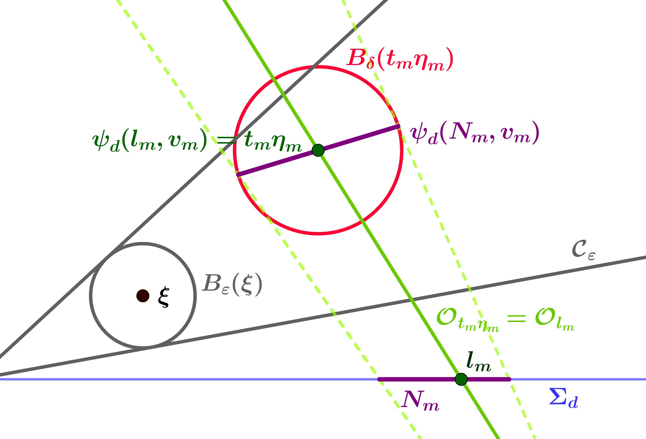
Figure 2. The choice of $l_{m}$ and $N_{m}$.

Applying the above Proposition 3.2 to $\zeta_{l}$, $l\in N_{m}$, we obtain measurable, normalized vectors $u_{\zeta_{l}},v_{\zeta_{l}}\in\mathcal{H}_{\zeta_{l}}$. Since $\sigma_{l}\cong\sigma_{\zeta_{l}}$ and $\mathcal{H}_{l}\cong\mathcal{H}_{\zeta_{l}}$ we have corresponding measurable, normalized vectors $u_{l},v_{l}\in\mathcal{H}_{l}$. With these we define

$$u^{(m)}:=(\mu_{\pi}(N_{m}))^{-\frac{1}{2}}\int_{\Sigma_{d}}\chi_{N_{m}}(l)u_{l}\leavevmode\nobreak\ d\mu_{\pi}(l)\;\in\mathcal{H}_{\pi},$$

since the $u_{l}$ are measurable in $l$ and $\|u^{(m)}\|^{2}_{\mathcal{H}_{\pi}}=(\mu_{\pi}(N_{m}))^{-1}\int_{\Sigma_{d}}\chi_{N_{m}}(l)\|u_{l}\|^{2}\leavevmode\nobreak\ d\mu_{\pi}(l)=1$. We define $v^{(m)}\in\mathcal{H}_{\pi}$ analogously.
Recall that Proposition 3.2 only gives us a lower bound for large $\|\zeta\|$ for functions $\phi$ with a small support, more precisely the support of $\phi$ shrinks proportional to $\langle\|\zeta\|\rangle^{-1/2}$. Thus, let $\varepsilon$ be as in Proposition 3.2 and $\phi\in C_{c}^{\infty}(B_{\varepsilon}(0))$ be non-negative, $\varphi=\phi\circ\log$. To adapt its support we define $\phi_{m}(X)\coloneq\langle t_{m}\rangle^{n/2}\phi(\langle t_{m}\rangle^{1/2}X)\in C_{c}^{\infty}(B_{\varepsilon\langle t_{m}\rangle^{-1/2}}(0))$, $\varphi_{m}=\phi_{m}\circ\log$. With this choice $\|\phi_{m}\|_{L^{1}}=\|\phi\|_{L^{1}}$ and $\|\phi_{m}\|_{W^{N,1}}\leq\langle t_{m}\rangle^{N/2}\|\phi\|_{W^{N,1}}$ Then, by definition of $N_{m}$:

$$|\mathcal{F}(\langle \pi(\bullet)u^{(m)},v^{(m)}\rangle\varphi_{m})(t_{m}\eta_{m})|$$

$$=\left|\int_{G}\int_{N_{m}}(\mu_{\pi}(N_{m}))^{-1}\langle\sigma_{l}(g)u_{l},v_{l}\rangle\varphi_{m}(g)e^{-2\pi t_{m}\eta_{m}(\log g)}\leavevmode\nobreak\ dg\leavevmode\nobreak\ d\mu_{\pi}(l)\right|$$

$$\geq\left|\operatorname{Re}\left(\int_{G}\int_{N_{m}}(\mu_{\pi}(N_{m}))^{-1}\langle\sigma_{l}(g)u_{l},v_{l}\rangle\varphi_{m}(g)e^{-2\pi t_{m}\eta_{m}(\log g)}\leavevmode\nobreak\ dg\leavevmode\nobreak\ d\mu_{\pi}(l)\right)\right|$$

$$=(\mu_{\pi}(N_{m}))^{-1}\left|\int_{N_{m}}\operatorname{Re}\left(\int_{\mathfrak{g}}\langle\sigma_{l}(\exp(X))u_{l},v_{l}\rangle\phi_{m}(X)e^{-2\pi t_{m}\eta_{m}(X)}\leavevmode\nobreak\ dX\right)\leavevmode\nobreak\ d\mu_{\pi}(l)\right|$$

$$\overset{\text{Prop. }\ref{prop:ReMcoeffsgeq}}{\geq}(\mu_{\pi}(N_{m}))^{-1}\int_{N_{m}}2^{-3\dim\mathfrak{g}}\|\phi_{m}\|_{L^{1}}\leavevmode\nobreak\ d\mu_{\pi}(l)=2^{-3\dim\mathfrak{g}}\|\phi\|_{L^{1}}\|u^{(m)}\|\|v^{(m)}\|.$$

We can use this to show that $\xi\in\operatorname{WF}(\pi)$: If we assume that $\xi\notin\operatorname{WF}(\pi)$ we can employ Lemma 2.4 (see also (6)). It states that there exist $\varepsilon_{1},\varepsilon_{2}>0$ such that for all $\varphi\in C_{c}^{\infty}(\exp(B_{\varepsilon_{2}}(0)))$ and all $N>n$:

$$|\mathcal{F}(\langle \pi(\bullet)u,v\rangle\varphi)(t\eta)|\leq C_{N}\|\varphi\|_{W^{N+n,1}}\|u\|\|v\|t^{-N}\quad\forall\;u,v\in\mathcal{H}_{\pi},\;\eta\in B_{\varepsilon_{1}}(\xi),\;t>t_{0}.$$

For our sequence chosen above this means we would have

$$|\mathcal{F}(\langle\pi(\bullet)u^{(m)} ,v^{(m)}\rangle\varphi_{m})(t_{m}\eta_{m})|\leq C_{N}\|\varphi_{m}\|_{W^{N+n,1}}\|u^{(m)}\|\|v^{(m)}\|t_{m}^{-N}$$

$$\leq C_{N}\|\varphi\|_{W^{N+n,1}}\|u^{(m)}\|\|v^{(m)}\|\langle t_{m}\rangle^{(N+n)/2}t_{m}^{-N}.$$

Since $\langle t_{m}\rangle^{(N+n)/2}t_{m}^{-N}\in\mathcal{O}\left(t_{m}^{(n-N)/2}\right)$ our estimations above show that this is not true for $N>n$.

∎

3.2. Proof of the Inclusion $\operatorname{WF}(\pi)\subset\operatorname{AC}(\mathcal{O}-\operatorname{supp}(\pi))$

For the proof of this inclusion we again find explicit microlocal estimates of individual matrix coefficients which we again obtain via induction over the dimension of $\mathfrak{g}$. For the formulation we use the notation introduced in Definition 2.12 once more.

Proposition 3.4.

Let $N$ be a nilpotent, connected, simply connected Lie group with Lie algebra $\mathfrak{n}$ and fix an inner product on $\mathfrak{g}_{0}$. Then for any $n,N\in\mathbb{N}$ with $N>n$ there exists a constant $C_{n,N}>0$ such that for all nilpotent, connected, simply connected Lie groups $G$ with Lie algebra $(\mathfrak{g},\langle,\rangle_{\mathfrak{g}})\prec(\mathfrak{n},\langle,\rangle_{\mathfrak{n}})$, $\dim\mathfrak{g}=n$, and for all $1>\varepsilon>0$ there exists a neighborhood $U\subset\mathfrak{g}$ of $0$ such that the following estimate holds for all $\phi\in C_{c}^{\infty}(U)$, $l,\eta\in i\mathfrak{g}^{\ast}$ and all $u,v\in\mathcal{H}_{l}$:

$$\left|\int_{\mathfrak{g}}\langle\sigma_{l}(\exp(X))u,v\rangle_{\mathcal{H}_{l}}\phi(X)e^{-2\pi\eta(X)}\leavevmode\nobreak\ dX\right|\leq C_{n,N}\|u\|_{\mathcal{H}_{l}}\|v\|_{\mathcal{H}_{l}}\|\phi\|_{W^{N+n,1}(\mathfrak{g})}\langle d(B_{\varepsilon\|\eta\|}(\eta),\mathcal{O}_{l})\rangle^{-N},$$

where $dX$ the measure associated to the inner product on $\mathfrak{g}$.

For the proof of Proposition 3.4 we distinguish the same two cases as in the proof of Proposition 3.2. We want to outline our approach in each case:

• If $l(Z)=0$ for an $Z\in\mathfrak{z}(\mathfrak{g})$, we consider $\overline{\mathfrak{g}}=\mathfrak{g}/(\mathbb{R}\cdot Z)$, $\overline{l}=\operatorname{pr}_{i\overline{\mathfrak{g}}^{\ast}}(l)$ and find that $\sigma_{l}|_{\overline{G}}\cong\sigma_{\overline{l}}$ analogously to Case I of Theorem 4. Thus, we can express the Fourier transform of the matrix coefficient of $\sigma_{l}$ in terms of the Fourier transform of the corresponding matrix coefficient of $\sigma_{\overline{l}}$ and apply the induction hypothesis. To find the desired estimate we use the orbit structure $\operatorname{pr}_{i\overline{\mathfrak{g}}^{\ast}}(\mathcal{O}_{l})=\mathcal{O}_{\overline{l}}$.

• If $\mathfrak{z}(\mathfrak{g})=\mathbb{R}\cdot Z$ and $l(Z)\neq 0$, Kirillov’s Lemma 2.7 gives us a subalgebra $\mathfrak{g}_{0}$, $l_{0}=\operatorname{pr}_{i\mathfrak{g}_{0}^{\ast}}(l)$. Since we are in Case II of Theorem 4 we know that $\sigma_{l}\cong\operatorname{Ind}_{G_{0}}^{G}(\sigma_{l_{0}})$. Thus, we can express the Fourier transform of the matrix coefficient of $\sigma_{l}$ using the Fourier transform of the corresponding matrix coefficient of $\sigma_{l_{0}}$, apply the induction hypothesis and use the orbit picture $\operatorname{pr}_{i\mathfrak{g}_{0}^{\ast}}(\mathcal{O}_{\zeta})=\bigsqcup_{t\in\mathbb{R}}(\operatorname{Ad}^{\ast}\exp tX)\mathcal{O}_{\zeta_{0}}$ and $\mathcal{O}_{\zeta}=\operatorname{pr}_{i\mathfrak{g}_{0}^{\ast}}^{-1}(\operatorname{pr}_{i\mathfrak{g}_{0}^{\ast}}(\mathcal{O}_{\zeta}))$ in the estimates. However, we again face some difficulties: In order to express the Fourier transform of the matrix coefficient of $\sigma_{l}$ using the Fourier transform of the corresponding matrix coefficient of $\sigma_{l_{0}}$ we use a chart $\mathfrak{g}\to G$ resulting from the decomposition $\mathfrak{g}=\mathfrak{g}_{0}\oplus\mathbb{R}X$ given by the Kirillov Lemma. In order to switch to the desired chart $\exp:\mathfrak{g}\to G$ we apply the Fourier inversion formula and use non-stationary phase. Due to the latter we have to consider neighborhoods whose radius grows proportional to the norm of its center. But this is no problem for us and actually matches the conical property of the wave front set and the asymptotic cone.

Proof.

We prove this statement by induction on $\dim\mathfrak{g}$. If $n=\dim\mathfrak{g}=1$ or 2, the group is abelian. In this case the irreducible unitary representations are one-dimensional, $\sigma_{l}(g)=e^{2\pi l(\log g)}$, and have a zero-dimensional orbit $\mathcal{O}_{l}=\{l\}$. We compute

$$\left|\int_{\mathfrak{g}}\langle\sigma_{l}(\exp X)u,v\rangle_{\mathbb{C}}\phi(X)e^{-2\pi\eta(X)}\leavevmode\nobreak\ dX\right|=\left|\int_{\mathfrak{g}}\phi(g)e^{2\pi(l-\eta)(X)}u\overline{v}\leavevmode\nobreak\ dX\right|=|\hat{\phi}(\eta-l)|\cdot|u|\cdot|v|.$$

Fixing an inner product on $\mathfrak{g}$ we obtain a corresponding one on $i\mathfrak{g}^{\ast}$. Now let $\{X_{i}\}_{i=1}^{n}$ be an orthogonal basis for $\mathfrak{g}$ and pick $j\in\{1,n\}$ such that $|(l-\eta)(X_{j})|$ is maximal.
With this choice we have for $N\in\mathbb{N}$ and $l\neq\eta$

$$|\hat{\phi}(\eta-l)| =\left|(2\pi(l-\eta)(X_{j}))^{-N}\int_{\mathfrak{g}}\phi(X)\partial_{X_{j}}^{N}e^{2\pi(l-\eta)(X)}dX\right|$$

$$\leq(2\pi)^{-N}|(l-\eta)(X_{j}))|^{-N}\int_{\mathfrak{g}}|\partial_{X_{j}}^{N}\phi(X)|dX$$

$$\leq(2\pi)^{-N}\sqrt{n}^{N}\|l-\eta\|^{-N}\|\phi\|_{W^{N,1}(\mathfrak{g})}\quad\leq C_{n,N}\langle d(\eta,l)\rangle^{-N}\|\phi\|_{W^{N+n,1}(\mathfrak{g})}.$$

The claim now follows with $U=\mathfrak{g}$ since $d(l,\eta)\geq d(B_{\varepsilon\|\eta\|}(\eta),l)$ for all $\varepsilon>0$.

Now we assume $n=\dim\mathfrak{g}\geq 3$. We will distinguish between the two cases:

Case I: $\boldsymbol{l(Z)=0}$ for an $\boldsymbol{Z\in\mathfrak{z}(\mathfrak{g})}$. Given the inner product on $\mathfrak{g}$ let $W<\mathfrak{g}$ be the subspace such that $\mathfrak{g}=W\oplus\mathbb{R}Z$ is an orthogonal decomposition. Then $\overline{\mathfrak{g}}=\mathfrak{g}/(\mathbb{R}\cdot Z)$ is isomorphic to $W$ and has a well-defined Lie algebra structure $[v+\mathbb{R}Z,w+\mathbb{R}Z]=[v,w]_{\mathfrak{g}}+\mathbb{R}Z$ since $Z\in\mathfrak{z}(\mathfrak{g})$.
Given an inner product on $\overline{\mathfrak{g}}$ we choose one on $\mathfrak{g}$ such that the decomposition above is orthogonal. Furthermore, without loss of generality we may assume $\|Z\|=1$. Using the corresponding inner product on $i\mathfrak{g}^{\ast}$ we also obtain an orthogonal decomposition $i\mathfrak{g}^{\ast}=iW^{\ast}\oplus\mathbb{R}\eta_{Z}\cong i\overline{\mathfrak{g}}^{\ast}\oplus\mathbb{R}\eta_{Z}$ with $\|\eta_{Z}\|=1$.
Note that $i\overline{\mathfrak{g}}^{\ast}$ is $\operatorname{Ad}^{\ast}(G)$-invariant (again due to $Z\in\mathfrak{z}(\mathfrak{g})$). We can identify $l$ and its orbit $\mathcal{O}_{l}^{G}\subset i\mathfrak{g}^{\ast}$ with an element $\overline{l}\in i\overline{\mathfrak{g}}^{\ast}$ and its orbit $\mathcal{O}_{\overline{l}}^{\overline{G}}\subset i\overline{\mathfrak{g}}^{\ast}$, respectively.
Let $\eta=\overline{\eta}+r\eta_{Z}\in i\mathfrak{g}^{\ast}=i\overline{\mathfrak{g}}^{\ast}\oplus\mathbb{R}\eta_{Z}$. Then by the choice of the inner product we know $d(\eta,\mathcal{O}_{l}^{G})^{2}=d(\overline{\eta},\mathcal{O}_{\overline{l}}^{\overline{G}})^{2}+r^{2}$ and assuming $d(B_{\varepsilon\|\eta\|}(\eta),\mathcal{O}_{l})>0$ we can estimate

$$d(B_{\varepsilon\|\eta\|}(\eta),\mathcal{O}_{l}) =d(\eta,\mathcal{O}_{l})-\varepsilon\|\eta\|=\sqrt{d(\overline{\eta},\mathcal{O}_{\overline{l}})^{2}+r^{2}}-\varepsilon\|\eta\|\leq d(\overline{\eta},\mathcal{O}_{\overline{l}})+r-\varepsilon\|\eta\|$$

$$\leq d(B_{\varepsilon\|\overline{\eta}\|}(\overline{\eta}),\mathcal{O}_{\overline{l}})+\varepsilon\|\overline{\eta}\|+r-\varepsilon\|\eta\|\leq d(B_{\varepsilon\|\overline{\eta}\|}(\overline{\eta}),\mathcal{O}_{\overline{l}})+r,$$

since $\|\overline{\eta}\|-\|\eta\|\leq 0$. This implies that we are either in the case

(10) $$\text{a) }r\geq\frac{1}{2}d(B_{\varepsilon\|\eta\|}(\eta),\mathcal{O}_{l}^{G})\quad\text{ or }\quad\text{b) }d(B_{\varepsilon\|\overline{\eta}\|}(\overline{\eta}),\mathcal{O}_{\overline{l}}^{\overline{G}})\geq\frac{1}{2}d(B_{\varepsilon\|\eta\|}(\eta),\mathcal{O}_{l}^{G}).$$

Turning to the integral we want to estimate:

$$J :=\left|\int_{\mathfrak{g}}\langle\sigma_{l}(\exp(X))u,v\rangle_{\mathcal{H}_{l}}\phi(X)e^{-2\pi\eta(X)}\leavevmode\nobreak\ dX\right|$$

$$=\left|\int_{\overline{\mathfrak{g}}}\int_{\mathbb{R}}\langle\sigma_{l}(\exp(\overline{X}+tZ))u,v\rangle_{\mathcal{H}_{l}}\phi(\overline{X}+tZ)e^{-2\pi\eta(\overline{X}+tZ)}d\overline{X}\leavevmode\nobreak\ dt\right|$$

$$=\left|\int_{\overline{\mathfrak{g}}}\int_{\mathbb{R}}\langle\sigma_{l}(\exp(\overline{X})\exp(tZ))u,v\rangle_{\mathcal{H}_{l}}\phi(\overline{X}+tZ)e^{-2\pi(\overline{\eta}(\overline{X})+r\eta_{Z}(tZ))}d\overline{X}\leavevmode\nobreak\ dt\right|$$

$$=\left|\int_{\overline{\mathfrak{g}}}\int_{\mathbb{R}}\langle\sigma_{l}(\exp(\overline{X}))u,v\rangle_{\mathcal{H}_{l}}\phi(\overline{X}+tZ)e^{-2\pi(\overline{\eta}(\overline{X})+r\eta_{Z}(tZ))}d\overline{X}\leavevmode\nobreak\ dt\right|$$

The last equality is due to $l(Z)=0$ which implies $\sigma_{l}(g\exp(tZ))=\sigma_{l}(g)$ for all $g\in G$, $t\in\mathbb{R}$.

We start with case a) of (10) and define

$$\tilde{\phi}(t):=\int_{\overline{\mathfrak{g}}}\langle\sigma_{l}(\exp(\overline{X}))u,v\rangle_{\mathcal{H}_{l}}\phi(\overline{X}+tZ)e^{-2\pi\overline{\eta}(\overline{X})}\leavevmode\nobreak\ d\overline{X}\;\in C_{c}^{\infty}(\mathbb{R}).$$

Then by integration by parts (as in the abelian case with $l=0$ and $u=v=1$) we obtain

$$J=\left|\int_{\mathbb{R}}\tilde{\phi}(t)e^{-2\pi rt}\leavevmode\nobreak\ dt\right|\leq C\|\tilde{\phi}\|_{W^{N,1}(\mathbb{R})}r^{-N}\overset{(\ref{eq:casesabd})a)}{\leq}C_{N}\|\tilde{\phi}\|_{W^{N+n,1}(\mathbb{R})}\langle d(B_{\varepsilon\|\eta\|}(\eta),\mathcal{O}_{l}^{G})\rangle^{-N}.$$

The claim now follows in this case with the following estimation:

$$\|\tilde{\phi}\|_{W^{N+n,1}(\mathbb{R})} =\sum_{k=1}^{N+n}\|\partial_{t}^{k}\tilde{\phi}\|_{L^{1}(\mathbb{R},dt)}$$

$$\leq\sum_{k=1}^{N+n}\int_{\mathbb{R}}\int_{\overline{\mathfrak{g}}}\left|\langle\sigma_{l}(\exp(\overline{X}))u,v\rangle_{\mathcal{H}_{l}}\partial_{t}^{k}\phi(\overline{X}+tZ)e^{-2\pi\overline{\eta}(\overline{X})}\right|\leavevmode\nobreak\ d\overline{X}\leavevmode\nobreak\ dt$$

$$\leq\|u\|\|v\|\sum_{k=1}^{N+n}\int_{\mathbb{R}}\int_{\overline{\mathfrak{g}}}\left|\partial_{t}^{k}\phi(\overline{X}+tZ)\right|\leavevmode\nobreak\ d\overline{X}\leavevmode\nobreak\ dt\quad\leq\quad\|u\|\|v\|\|\phi\|_{W^{N+n,1}(\mathfrak{g})}.$$

Now let’s turn to case b) of (10). Note that by Theorem 4 (i) we know $\mathcal{H}_{l}\cong\mathcal{H}_{\overline{l}}$ and $\sigma_{\overline{l}}\circ P\cong\sigma_{l}$ with the projection $P:G\to\overline{G}$.
Thus, we have

$$J =\left|\int_{\overline{\mathfrak{g}}}\int_{\mathbb{R}}\langle\sigma_{\overline{l}}(\exp(\overline{X}))u,v\rangle_{\mathcal{H}_{\overline{l}}}\phi(\overline{X}+tZ)e^{-2\pi(\overline{\eta}(\overline{X})+r\eta_{Z}(tZ))}d\overline{X}\leavevmode\nobreak\ dt\right|.$$

Now define

$$\check{\phi}(\overline{X}):=\int_{\mathbb{R}}\phi(\overline{X}+tZ)e^{-2\pi irt}\leavevmode\nobreak\ dt\;\in C_{c}^{\infty}(\overline{\mathfrak{g}}),$$

and choose the neighborhood $0\in U\subset\mathfrak{g}$ such that $\operatorname{supp}\check{\phi}\subset\overline{U}\subset\overline{\mathfrak{g}}$ given by the induction hypothesis applied to $\overline{\mathfrak{g}}$. Then

$$J =\left|\int_{\overline{\mathfrak{g}}}\langle\sigma_{\overline{l}}(\exp(\overline{X}))u,v\rangle_{\mathcal{H}_{l}}\check{\phi}(\overline{X})e^{-2\pi\overline{\eta}(\overline{X})}d\overline{X}\right|$$

$$\overset{\text{(IH)}}{\leq}C_{n-1,N}\|u\|\|v\|\|\check{\phi}\|_{W^{N+n-1,1}(\overline{\mathfrak{g}})}\langle d(B_{\varepsilon\|\overline{\eta}\|}(\overline{\eta}),\mathcal{O}_{\overline{l}}^{\overline{G}})\rangle^{-N}$$

$$\overset{(\ref{eq:casesabd})b)}{\leq}C_{n,N}\|u\|\|v\|\|\check{\phi}\|_{W^{N+n,1}(\overline{\mathfrak{g}})}\langle d(B_{\varepsilon\|\eta\|}(\eta),\mathcal{O}_{l}^{G})\rangle^{-N}.$$

The claim now follows in this case with the following estimation:

$$\|\check{\phi}\|_{W^{N+n,1}(\overline{\mathfrak{g}})} =\sum_{|\alpha|<N+n}\|\partial^{\alpha}\check{\phi}\|_{L^{1}(\overline{\mathfrak{g}},dv)}$$

$$=\sum_{\alpha}\int_{\overline{\mathfrak{g}}}\left|\int_{\mathbb{R}}\partial_{\overline{X}}^{\alpha}\phi(\overline{X}+tZ)e^{-2\pi irt}\leavevmode\nobreak\ dt\right|\leavevmode\nobreak\ d\overline{X}$$

$$\leq\sum_{\alpha}\int_{\overline{\mathfrak{g}}}\int_{\mathbb{R}}\left|\partial_{\overline{X}}^{\alpha}\phi(\overline{X}+tZ)\right|\leavevmode\nobreak\ dt\leavevmode\nobreak\ d\overline{X}\quad\leq\quad\|\phi\|_{W^{N+n,1}(\mathfrak{g})}.$$

Case II: $\boldsymbol{\mathfrak{z}(\mathfrak{g})=\mathbb{R}\cdot Z}$ and $\boldsymbol{l(Z)\neq 0}$. Kirillov’s Lemma 2.7 gives us $X,Y\in\mathfrak{g}$ and an ideal $\mathfrak{g}_{0}\subset\mathfrak{g}$ with $\mathfrak{g}=\mathbb{R}X\oplus\mathfrak{g}_{0}$ and $[X,Y]=Z$. We may choose $X$ such that this decomposition is orthogonal. Since $\dim(\mathfrak{z}(\mathfrak{g}_{0}))>1$ as $Z,Y\in\mathfrak{z}(\mathfrak{g}_{0})$ we are in Case I in the induction hypotheses for $G_{0}$ . We define a chart for $G$ via

$$\beta:\mathfrak{g}=\mathfrak{g}_{0}\oplus\mathbb{R}X\to G,\quad X_{0}+tX\mapsto\exp(X_{0})\exp(tX).$$

Since $X\notin\mathfrak{r}_{l}$ and we are in Case II of Proposition 2.11 and Theorem 4:

$$p:i\mathfrak{g}^{\ast}\to i\mathfrak{g}^{\ast}_{0},\quad l_{0}:=p(l),\eta_{0}:=p(\eta),\;\mathcal{O}_{l_{0}}^{G_{0}}:=\operatorname{Ad}^{\ast}(G_{0})l_{0},$$

$$p(\mathcal{O}_{l}^{G})=\bigsqcup_{t\in\mathbb{R}}(\operatorname{Ad}^{\ast}\exp tX)\mathcal{O}_{l_{0}}^{G_{0}},\quad\mathcal{O}_{l}^{G}=p^{-1}(p(\mathcal{O}_{l}^{G})).$$

where $G_{0}=\exp(\mathfrak{g}_{0})\subset G$ is a normal subgroup. Note that we also have an orthogonal decomposition $\mathfrak{g}^{\ast}=\mathbb{R}\eta_{X}\oplus\mathfrak{g}^{\ast}_{0}$, $\eta_{X}(X)=1$, which gives us for all $a\in A=\exp(\mathbb{R}X)$:

$$d(\eta_{0},\mathcal{O}_{\operatorname{Ad}^{\ast}(a)l_{0}}^{G_{0}})=d(\eta_{0},\operatorname{Ad}^{\ast}(a)\mathcal{O}_{l_{0}}^{G_{0}})\geq d(\eta_{0},p(\mathcal{O}_{l}^{G}))=d(\eta,\mathcal{O}_{l}^{G}).$$

Assuming $d(B_{\varepsilon\|\eta\|}(\eta),\mathcal{O}_{l}^{G})>0$ we can estimate

(11) $$d(B_{\varepsilon\|\eta\|}(\eta),\mathcal{O}_{l}^{G}) =d(\eta,\mathcal{O}_{l}^{G})-\varepsilon\|\eta\|\leq d(\eta_{0},\mathcal{O}_{\operatorname{Ad}^{\ast}(a)l_{0}}^{G_{0}})-\varepsilon\|\eta\|$$

$$=d(B_{\varepsilon\|\eta_{0}\|}(\eta_{0}),\mathcal{O}_{\operatorname{Ad}^{\ast}(a)l_{0}}^{G_{0}})+\varepsilon\|\eta_{0}\|-\varepsilon\|\eta\|\leq d(B_{\varepsilon\|\eta_{0}\|}(\eta_{0}),\mathcal{O}_{\operatorname{Ad}^{\ast}(a)l_{0}}^{G_{0}}),$$

since $\|\eta_{0}\|-\|\eta\|\leq 0$. In addition to that we have $\eta=\eta_{0}+\eta_{X}$ with $\eta_{X}\in\ker(p)$.

We start by estimating the following integral and deal with the transition from the chart $\beta$ to the exponential chart later on.

$$J(\phi,\eta) :=\left|\int_{\mathfrak{g}}\langle\sigma_{l}(\beta(X))u,v\rangle_{\mathcal{H}_{l}}\phi(X)e^{-2\pi\eta(X)}\leavevmode\nobreak\ dX\right|$$

$$=\left|\int_{\mathfrak{g}_{0}}\int_{\mathbb{R}}\langle\sigma_{l}(\exp(X_{0})\exp(tX))u,v\rangle_{\mathcal{H}_{l}}\phi(X_{0}+tX)e^{-2\pi(\eta_{0}(X_{0})+r\eta_{X}(tX))}dX_{0}\leavevmode\nobreak\ dt\right|.$$

By Theorem 4, we also know $\sigma_{l}\cong\operatorname{Ind}_{G_{0}}^{G}(\sigma_{l_{0}})$. Note that $\mathcal{H}_{l}\cong L^{2}(A,\mathcal{H}_{l_{0}})$. If we regard $u$ and $v$ as elements of $L^{2}(A,\mathcal{H}_{l_{0}})$ and $\tilde{u},\tilde{v}:G\to\mathcal{H}_{l_{0}}$ the corresponding functions in the ’standard model’ we have again

$$\langle\sigma_{l}(g_{0}a)u,v\rangle_{\mathcal{H}_{l}}=\int_{A}\langle[\sigma_{l}(g_{0}a)u](b),v(b)\rangle_{\mathcal{H}_{l_{0}}}\leavevmode\nobreak\ db\quad\text{ and }$$

$$[\sigma_{l}(g_{0}a)\tilde{u}](b)=\tilde{u}(bg_{0}a)=\tilde{u}(bg_{0}b^{-1}ba)=\sigma_{l_{0}}(bg_{0}b^{-1})\tilde{u}(ba)$$

since $b^{-1}g_{0}b\in G_{0}$ as $\mathfrak{g}_{0}$ is an ideal. This gives us $[\sigma_{l}(g_{0}a)u](b)=\sigma_{l_{0}}(bg_{0}b^{-1})u(ba)$.
We deduce that

$$J(\phi,\eta) =\bigg{|}\int_{\mathfrak{g}_{0}}\int_{\mathbb{R}}\left(\int_{A}\langle\sigma_{l_{0}}(b\exp(X_{0})b^{-1})u(be^{tX}),v(b)\rangle_{\mathcal{H}_{l_{0}}}db\right)\cdot$$

$$\qquad\qquad\qquad\qquad\qquad\qquad\qquad\qquad\qquad\quad\phi(X_{0}+tX)e^{-2\pi(\eta_{0}(X_{0})+r\eta_{X}(tX))}dX_{0}\leavevmode\nobreak\ dt\bigg{|}$$

$$\leq\int_{\mathbb{R}}\int_{A}\left|\int_{\mathfrak{g}_{0}}\langle\sigma_{l_{0}}(b\exp(X_{0})b^{-1})u(be^{tX}),v(b)\rangle_{\mathcal{H}_{l_{0}}}\phi(X_{0}+tX)e^{-2\pi\eta_{0}(X_{0})}dX_{0}\right|\cdot$$

$$\qquad\qquad\qquad\qquad\qquad\qquad\qquad\qquad\qquad\qquad\qquad\qquad\qquad\qquad\left|e^{-2\pi r\eta_{X}(tX)}\right|db\leavevmode\nobreak\ dt.$$

The conjugation $C_{b}:G_{0}\to G_{0},g_{0}\mapsto b^{-1}g_{0}b$ is a group automorphism and we know that $\chi_{l_{0}}\circ C_{b}=\chi_{\operatorname{Ad}^{\ast}(b)l_{0}}$ for the character $\chi_{l_{0}}$ such that $\sigma_{l_{0}}=\operatorname{Ind}_{M}^{G_{0}}(\chi_{l_{0}})$, $M=\exp(\mathfrak{m})$ for a polarizing subalgebra $\mathfrak{m}\subset\mathfrak{g}_{0}$. Now, $\operatorname{Ad}(b)\mathfrak{m}$ is a polarizing subalgebra for $\operatorname{Ad}^{\ast}(b)l_{0}$ and $C_{b}^{-1}M=\exp(\operatorname{Ad}(b)\mathfrak{m})$. Thus, [CG90, Lemma 2.1.3] gives us

$$\sigma_{\operatorname{Ad}^{\ast}(b)l_{0}}=\operatorname{Ind}_{C_{b}^{-1}M}^{G_{0}}(\chi_{l_{0}}\circ C_{b})\cong\operatorname{Ind}_{M}^{G_{0}}(\chi_{l_{0}})\circ C_{b}=\sigma_{l_{0}}\circ C_{b}.$$

We choose $U\subset\mathfrak{g}$ such that for all $\phi\in C_{c}^{\infty}(U)$ and $X_{0}+tX\in U$ we have $\operatorname{supp}(\phi(\bullet+tX))\subset U_{0}\subset\mathfrak{g}_{0}$, where $0\in U_{0}\subset\mathfrak{g}_{0}$ is given by the induction hypothesis for $G_{0}$. We apply it to $\operatorname{Ad}^{\ast}(b^{-1})l_{0}$ instead of $l_{0}$:

$$J (\phi,\eta)\leq\int_{\mathbb{R}}\int_{A}\left|\int_{\mathfrak{g}_{0}}\langle\sigma_{l_{0}}(b\exp(X_{0})b^{-1})u(be^{tX}),v(b)\rangle_{\mathcal{H}_{l_{0}}}\phi(X_{0}+tX)e^{-2\pi\eta_{0}(X_{0})}dX_{0}\right|\cdot$$

$$\qquad\qquad\qquad\qquad\qquad\qquad\qquad\qquad\qquad\qquad\qquad\qquad\qquad\qquad\qquad\qquad\left|e^{-2\pi r\eta_{X}(tX)}\right|db\leavevmode\nobreak\ dt$$

$$\overset{\text{(IH)}}{\leq}\int_{\mathbb{R}}\int_{A}C_{n-1,N}\|\phi(\bullet+tX)\|_{W^{N+n-1,1}(\mathfrak{g}_{0})}\|u(be^{tX})\|_{\mathcal{H}_{l_{0}}}\|v(b)\|_{\mathcal{H}_{l_{0}}}\cdot$$

$$\qquad\qquad\qquad\qquad\qquad\qquad\qquad\qquad\qquad\qquad\qquad\qquad\langle d(B_{\varepsilon\|\eta_{0}\|}(\eta_{0}),\mathcal{O}_{\operatorname{Ad}^{\ast}(b^{-1})l_{0}}^{G_{0}})\rangle^{-N}\leavevmode\nobreak\ db\leavevmode\nobreak\ dt$$

$$\overset{(\ref{eq:d0})}{\leq}C_{n-1,N}\langle d(B_{\varepsilon\|\eta\|}(\eta),\mathcal{O}_{l})\rangle^{-N}\int_{\mathbb{R}}\left(\int_{A}\|T_{\exp(tX)}u(b)\|_{\mathcal{H}_{l_{0}}}\|v(b)\|_{\mathcal{H}_{l_{0}}}\leavevmode\nobreak\ db\right)\|\phi(\bullet+tX)\|_{W^{N+n-1,1}}\leavevmode\nobreak\ dt$$

$$\leq\;C_{n-1,N}\langle d(B_{\varepsilon\|\eta\|}(\eta),\mathcal{O}_{l})\rangle^{-N}\int_{\mathbb{R}}\|T_{\exp(tX)}u\|_{\mathcal{H}_{l}}\|v\|_{\mathcal{H}_{l}}\|\phi(\bullet+tX)\|_{W^{N+n,1}(\mathfrak{g}_{0})}\leavevmode\nobreak\ dt,$$

where $T_{\exp(tX)}$ is the translation by $\exp(tX)\in A$ which is an isometry on $\mathcal{H}_{l}\cong L^{2}(A,\mathcal{H}_{l_{0}})$. This gives us

$$J(\phi,\eta) \leq\;C_{n,N}\langle d(B_{\varepsilon\|\eta\|}(\eta),\mathcal{O}_{l})\rangle^{-N}\|u\|_{\mathcal{H}_{l}}\|v\|_{\mathcal{H}_{l}}\int_{\mathbb{R}}\|\phi(\bullet+tX)\|_{W^{N+n,1}(\mathfrak{g}_{0})}\leavevmode\nobreak\ dt$$

$$=\;C_{n,N}\langle d(B_{\varepsilon\|\eta\|}(\eta),\mathcal{O}_{l})\rangle^{-N}\|u\|_{\mathcal{H}_{l}}\|v\|_{\mathcal{H}_{l}}\int_{\mathbb{R}}\sum_{|\alpha|\leq N+n}\int_{\mathfrak{g}_{0}}|\partial_{X_{0}}^{N}\phi(X_{0}+tX)|dX_{0}\leavevmode\nobreak\ dt$$

$$\leq\;C_{n,N}\langle d(B_{\varepsilon\|\eta\|}(\eta),\mathcal{O}_{l})\rangle^{-N}\|u\|_{\mathcal{H}_{l}}\|v\|_{\mathcal{H}_{l}}\|\phi\|_{W^{N+n,1}(\mathfrak{g})},$$

Now let $\kappa=\beta^{-1}\circ\exp:\mathfrak{g}\to\mathfrak{g}$ be the transition map. Then the integral we are interested in can be written as

$$F :=\left|\int_{\mathfrak{g}}\langle\sigma_{l}(\exp(X))u,v\rangle_{\mathcal{H}_{l}}\phi(X)e^{-2\pi\eta(X)}\leavevmode\nobreak\ dX\right|$$

$$=\left|\int_{\mathfrak{g}}\langle\sigma_{l}(\beta(\kappa(X)))u,v\rangle_{\mathcal{H}_{l}}\chi(X)\phi(X)e^{-2\pi\eta(X)}\leavevmode\nobreak\ dX\right|,$$

where $\chi\in C_{c}^{\infty}(\mathfrak{g})$ is a cut-off function with $\chi=1$ on $\operatorname{supp}(\phi)$. The Fourier inversion formula yields

$$F =\left|\int_{i\mathfrak{g}^{\ast}}\mathcal{F}\left(\langle\sigma_{l}(\beta(\bullet))u,v\rangle_{\mathcal{H}_{l}}\chi(\bullet)\right)(\xi)\int_{\mathfrak{g}}\phi(X)e^{-2\pi(\eta(X)-\xi(\kappa(X))}\leavevmode\nobreak\ dX\leavevmode\nobreak\ d\xi\right|.$$

Now, $\mathcal{F}\left(\sigma_{l}(\beta(\bullet))u,v\rangle_{\mathcal{H}_{l}}\chi(\bullet)\right)(\xi)=J(\chi,\xi)$ from above. Furthermore, we can use non-stationary phase to estimate the inner integral

$$I(\phi,\xi,\eta):=\int_{\mathfrak{g}}\phi(X)e^{-2\pi(\eta(X)-\xi(\kappa(X))}\leavevmode\nobreak\ dX=\int_{\mathfrak{g}}\phi(X)e^{-2\pi d_{\varepsilon}(\eta(X)-\xi(\kappa(X))/d_{\varepsilon}}\leavevmode\nobreak\ dX,$$

where $d_{\varepsilon}=d(B_{\varepsilon\|\xi\|}(\xi),\eta)>0$ is assumed. With the phase function $f_{\xi,\eta}(X):=\frac{1}{d_{\varepsilon}}(\eta(X)-\xi(\kappa(X))$ we have $d_{X}f_{\xi,\eta}(X):=\frac{1}{d_{\varepsilon}}(\eta-\xi\circ D\kappa(X)))$ where $D\kappa(X):\mathfrak{g}\to\mathfrak{g}$ is the differential of $\kappa$ in $X$. Since $D\kappa(0)=1$ we have

$$\|\xi\circ D\kappa(X)-\xi\|\leq\sup_{X\in U}\|D\kappa(X)-1\|\|\xi\|\leq\varepsilon\|\xi\|,$$

after possibly shrinking the neighborhood $0\in U\subset\mathfrak{g}$. This gives us

$$\|\eta-\xi\circ D\kappa(X)\|\geq\|\eta-\xi\|-\varepsilon\|\xi\|=d_{\varepsilon}\quad\Rightarrow\quad\left|d_{X}f_{\xi,\eta}(X)\right|\geq 1.$$

With [Hör03, Theorem 7.7.1] we can estimate

$$|I(\phi,\xi,\eta)|\leq C_{N}\|\kappa\|_{C^{N+1}}\|\phi\|_{W^{N,1}(\mathfrak{g})}d(B_{\varepsilon\|\xi\|}(\xi),\eta)^{-N}.$$

Note that Hörmander uses on the right hand side instead of the Sobolev norm of $\phi$ the term $\sum_{|\alpha|\leq N}\sup_{X}|D^{\alpha}\phi(X)|$. But when you take a closer look at his proof one finds that these suprema occur as an estimate of the integral of $\phi$. Hence, they can be replaced by the Sobolev norm. Furthermore, by Lemma 2.13 we have $\|\kappa\|_{C^{N+1}}\leq C_{\mathfrak{g},N}\leq C_{\mathfrak{n},N}$ and therefore can be absorbed into the constant $C_{N}$ (since this may depend on $\mathfrak{n}$ in our statement).
In order to prove the desired estimate it suffices to prove it in the case that $d(B_{\varepsilon\|\eta\|}(\eta),\mathcal{O}_{l})>0$ which is equal to

(12) $$\varepsilon\|\eta\|<d(\eta,\mathcal{O}_{l})$$

and implies that $\frac{1}{2}d:=\frac{1}{2}d(\eta,\mathcal{O}_{l})<d(B_{\varepsilon/3\|\eta\|}(\eta),\mathcal{O}_{l})=:d_{\varepsilon/3}$. Now, we split up the integral:

$$F_{I}:=\left|\int_{B(1/2d_{\varepsilon/3},\eta)}J(\chi,\xi)I(\phi,\xi,\eta)\leavevmode\nobreak\ d\xi\right|,\quad F_{II}:=\left|\int_{i\mathfrak{g}^{\ast}\setminus B(d/4,\eta)}J(\chi,\xi)I(\phi,\xi,\eta)\leavevmode\nobreak\ d\xi\right|.$$

Since the two domains of integration are overlapping we have $F\leq F_{I}+F_{II}$.
With the estimates above (with $\frac{\varepsilon}{9}$ instead of $\varepsilon$) we obtain

$$F_{I} \leq C_{n,N}\langle d(B_{\varepsilon/9\|\xi\|}(\xi),\mathcal{O}_{l})\rangle^{-N}\|u\|_{\mathcal{H}_{l}}\|v\|_{\mathcal{H}_{l}}\|\chi\|_{W^{N+n,1}(\mathfrak{g})}\|\phi\|_{L^{1}(\mathfrak{g})}d_{\varepsilon/3}^{n}.$$

For all $\xi\in B_{R}(\eta)$, $R=\frac{1}{2}d_{\varepsilon/3}\leq\frac{1}{2}d(\eta,\mathcal{O}_{l})$, we can estimate

(13) $$d(B_{\varepsilon/9\|\xi\|}(\xi),\mathcal{O}_{l}) \geq d(\eta,\mathcal{O}_{l})-R-\frac{\varepsilon}{9}\|\xi\|\geq d(\eta,\mathcal{O}_{l})-(1+\varepsilon/9)R-\frac{\varepsilon}{9}\|\eta\|$$

$$\geq\frac{1}{3}(d(\eta,\mathcal{O}_{l})-\varepsilon/3\|\eta\|)=\frac{1}{3}d(B_{\varepsilon/3\|\eta\|}(\eta),\mathcal{O}_{l}).$$

This gives us

$$F_{I} \leq C_{n,N}\langle d(B_{\varepsilon/3\|\eta\|}(\eta),\mathcal{O}_{l})\rangle^{-N+n}\|u\|_{\mathcal{H}_{l}}\|v\|_{\mathcal{H}_{l}}\|\phi\|_{W^{N,1}(\mathfrak{g})}$$

$$\leq C_{n,N}\langle d(B_{\varepsilon\|\eta\|}(\eta),\mathcal{O}_{l})\rangle^{-N+n}\|u\|_{\mathcal{H}_{l}}\|v\|_{\mathcal{H}_{l}}\|\phi\|_{W^{N,1}(\mathfrak{g})},$$

since $d(B_{\varepsilon\|\eta\|}(\eta),\mathcal{O}_{l})\leq d(B_{\varepsilon/3\|\eta\|}(\eta),\mathcal{O}_{l})$ and $-N+n<0$.
For the second part we use the above estimates again with $\frac{\varepsilon}{9}$ instead of $\varepsilon$:

$$F_{II} \leq C_{N}\|\phi\|_{W^{N,1}(\mathfrak{g})}\|\chi\|_{L^{1}(\mathfrak{g})}\|u\|_{\mathcal{H}_{l}}\|v\|_{\mathcal{H}_{l}}\int_{i\mathfrak{g}^{\ast}\setminus B(d/4,\eta)}d(B_{\varepsilon/9\|\xi\|}(\xi),\eta)^{-N}\leavevmode\nobreak\ d\xi.$$

We estimate with $r=\|\xi-\eta\|\geq\frac{1}{4}d(\eta,\mathcal{O}_{l})$ and $\varepsilon<1$

$$d(B_{\varepsilon/9\|\xi\|}(\xi),\eta) =\|\xi-\eta\|-\frac{\varepsilon}{9}\|\xi\|\geq\left(1-\frac{\varepsilon}{9}\right)r-\frac{\varepsilon}{9}\|\eta\|\overset{\eqref{eq:epseta<d}}{\geq}\left(1-\frac{\varepsilon}{9}\right)r-\frac{1}{9}d(\eta,\mathcal{O}_{l})$$

$$\geq\left(1-\frac{\varepsilon}{9}-\frac{4}{9}\right)r\geq\frac{4}{9}r$$

and therefore with polar coordinates

$$F_{II} \leq C_{N}\|\phi\|_{W^{N,1}(\mathfrak{g})}\|u\|_{\mathcal{H}_{l}}\|v\|_{\mathcal{H}_{l}}\left(\frac{4}{9}\right)^{N}\int_{d/4}^{\infty}r^{-N+n-1}\leavevmode\nobreak\ dr$$

$$=C_{N}\|\phi\|_{W^{N,1}(\mathfrak{g})}\|u\|_{\mathcal{H}_{l}}\|v\|_{\mathcal{H}_{l}}\frac{1}{4^{N-n}}d(\eta,\mathcal{O}_{l})^{-N+n}$$

$$\leq C_{n,N}\|\phi\|_{W^{N,1}(\mathfrak{g})}\|u\|_{\mathcal{H}_{l}}\|v\|_{\mathcal{H}_{l}}d(B_{\varepsilon\|\eta\|}(\eta),\mathcal{O}_{l})^{-N+n},$$

since $d(B_{\varepsilon\|\eta\|}(\eta),\mathcal{O}_{l})\leq d(\eta,\mathcal{O}_{l})$ and $-N+n<0$. ∎

Corollary 3.5.

The statement of the previous Proposition 3.4 also holds for $u,v\in\mathcal{H}_{l}^{\oplus m_{l}}$ with multiplicity $m_{l}\in\mathbb{N}\cup\{\infty\}$.

Proof.

For $u\in\mathcal{H}_{l}^{\oplus m_{l}}$ we have $u=(u_{1},u_{2},\ldots)$ with (finitely or infinitely many) $0\neq u_{i}\in\mathcal{H}_{l}$ and $\sum_{i}\|u_{i}\|^{2}_{\mathcal{H}_{l}}<\infty$, $\|u\|=\left(\sum_{i}\|u_{i}\|^{2}\right)^{1/2}$. Thus

$$\big{|}\int_{\mathfrak{g}}\langle\sigma_{l}(\exp(X))u,v\rangle_{\mathcal{H}_{l}} \phi(X)e^{-2\pi\eta(X)}\leavevmode\nobreak\ dX\big{|}=\left|\int_{\mathfrak{g}}\sum_{i}\langle\sigma_{l}(\exp(X))u_{i},v_{i}\rangle_{\mathcal{H}_{l}}\phi(X)e^{-2\pi\eta(X)}\leavevmode\nobreak\ dX\right|$$

$$=\left|\sum_{i}\int_{\mathfrak{g}}\langle\sigma_{l}(\exp(X))u_{i},v_{i}\rangle_{\mathcal{H}_{l}}\phi(X)e^{-2\pi\eta(X)}\leavevmode\nobreak\ dX\right|$$

$$\overset{\text{Prop. }\ref{prop:detaO}}{\leq}C_{n,N}\|\phi\|_{W^{N+n,1}(\mathfrak{g})}\langle d(B_{\varepsilon\|\eta\|}(\eta),\mathcal{O}_{l})\rangle^{-N}\sum_{i}\|u_{i}\|\cdot\|v_{i}\|$$

$$\leq C_{n,N}\|\phi\|_{W^{N+n,1}(\mathfrak{g})}\langle d(B_{\varepsilon\|\eta\|}(\eta),\mathcal{O}_{l})\rangle^{-N}\left(\sum_{i}\|u_{i}\|^{2}\right)^{1/2}\cdot\left(\sum_{i}\|v_{i}\|^{2}\right)^{1/2}$$

$$=C_{n,N}\|\phi\|_{W^{N+n,1}(\mathfrak{g})}\langle d(B_{\varepsilon\|\eta\|}(\eta),\mathcal{O}_{l})\rangle^{-N}\|u\|\cdot\|v\|,$$

where the interchanging of the order of integration and summation in the second equality is possible since $|\langle\sigma_{l}(\exp(X))u_{i},v_{i}\rangle\phi(X)e^{-2\pi\eta(X)}|\leq\|u_{i}\|\cdot\|v_{i}\|\cdot|\phi(X)|\in L^{1}(\mathbb{N}\times\mathfrak{g})$. ∎

This inequality whose constant is in particular independent of $l\in i\mathfrak{g}^{\ast}$ now helps us to estimate the matrix coefficients of the big unitary representation $\pi$ using its direct integral decomposition into the irreducibles $\sigma_{l}$.

Theorem 6.

Let $G$ be a nilpotent, connected, simply connected Lie group with Lie algebra $\mathfrak{g}$ and $(\pi,\mathcal{H}_{\pi})$ a unitary representation of $G$. Then

$$\operatorname{WF}(\pi)\subset\operatorname{AC}(\mathcal{O}-\operatorname{supp}\pi).$$

Proof.

Let $\eta\notin\operatorname{AC}(\mathcal{O}-\operatorname{supp}\pi)$, w.l.o.g. $\|\eta\|=1$. Then there exists $\varepsilon>0$ and $t_{0}>0$ such that $d(t\eta,\mathcal{O}-\operatorname{supp}\pi)\geq 2\varepsilon t$ for all $t\geq t_{0}$. In particular, for all $l\in\operatorname{supp}\pi$ we know $d(t\eta,\mathcal{O}_{l})\geq 2\varepsilon t$ which implies $d(B_{\varepsilon t}(t\eta),\mathcal{O}_{l})\geq\varepsilon t$.
Again, we use $\mathcal{H}_{\pi}=\int_{\Sigma_{d}}\mathcal{H}_{l}^{\oplus m(\pi,\sigma_{l})}\leavevmode\nobreak\ d\mu_{\pi}(l)$ for the Hilbert space of the unitary representation $\pi$. If $u=(u_{l}),v=(v_{l})\in\mathcal{H}$, $u_{l},v_{l}\in\mathcal{H}_{l}^{\oplus m(\pi,\sigma_{l})}$, in this direct integral decomposition the matrix coefficient is

$$\langle\pi(g)u,v\rangle=\int_{\Sigma_{d}}\langle\sigma_{l}(g)u_{l},v_{l}\rangle\leavevmode\nobreak\ d\mu_{\pi}(l).$$

Let $U\subset\mathfrak{g}$ be the neighborhood of $0$ from Proposition 3.4/Corollary 3.5 with $\varepsilon$ as chosen above and let $\phi\in C_{c}^{\infty}(U)$ with $\phi(0)\neq 0$. For $t\geq t_{0}$ and $\varphi:=\phi\circ\log\in C_{c}^{\infty}(G)$, $\varphi(e)\neq 0$, we conclude

$$|\mathcal{F}(\langle\pi(\bullet)u,v\rangle\varphi)(t\eta)| =\left|\int_{G}\langle\pi(g)u,v\rangle\varphi(g)e^{-2\pi t\eta(\log g)}\leavevmode\nobreak\ dg\right|$$

$$=\left|\int_{G}\int_{\Sigma_{d}}\langle\sigma_{l}(g)u_{l},v_{l}\rangle\varphi(g)e^{-2\pi t\eta(\log g)}\leavevmode\nobreak\ d\mu_{\pi}(l)\leavevmode\nobreak\ dg\right|$$

$$=\left|\int_{\Sigma_{d}}\left(\int_{G}\langle\sigma_{l}(g)u_{l},v_{l}\rangle\phi(\log g)e^{-2\pi t\eta(\log g)}\leavevmode\nobreak\ dg\right)\leavevmode\nobreak\ d\mu_{\pi}(l)\right|$$

$$\leq\int_{\Sigma_{d}}\left|\int_{\mathfrak{g}}\langle\sigma_{l}(\exp(X))u_{l},v_{l}\rangle\phi(X)e^{-2\pi t\eta(X)}\leavevmode\nobreak\ dX\right|\leavevmode\nobreak\ d\mu_{\pi}(l)$$

$$\overset{\text{Cor. }\ref{cor:deta0}}{\leq}\int_{\Sigma_{d}}C_{n,N}\|u\|_{\mathcal{H}_{l}}\|v\|_{\mathcal{H}_{l}}\|\phi\|_{W^{N+n,1}(\mathfrak{g})}\langle d(B_{\varepsilon t}(t\eta),\mathcal{O}_{l})\rangle^{-N}\leavevmode\nobreak\ d\mu_{\pi}(l)$$

$$\leq C_{n,N}\|\phi\|_{W^{N,1}(\mathfrak{g})}\varepsilon^{-N}t^{-N}\int_{\Sigma_{d}}\|u_{l}\|\cdot\|v_{l}\|\leavevmode\nobreak\ d\mu_{\pi}(l)$$

$$\leq C_{n,N}\|\phi\|_{W^{N,1}(\mathfrak{g})}\varepsilon^{-N}\|u\|_{\mathcal{H}_{\pi}}\cdot\|v\|_{\mathcal{H}_{\pi}}t^{-N}.$$

This implies $\eta\notin\operatorname{WF}_{e}(\langle\pi(\bullet)u,v\rangle)$. ∎

References

- [Bro73] Ian D. Brown, Dual topology of a nilpotent Lie group, Annales scientifiques de l’École Normale Supérieure 6 (1973), no. 3, 407–411.
- [Bud21] Julia Budde, Wave front sets of nilpotent Lie group representations, 2021.
- [CG90] Lawrence J. Corwin and Frederick P. Greenleaf, Representations of Nilpotent Lie Groups and Their Application. Part 1: Basic Theory and Examples, Cambridge Studies in Advanced Mathematics, Cambridge University Press, 1990.
- [DK01] Johannes J. Duistermaat and Johann A.C. Kolk, Lie Groups, Universitext, Springer Berlin Heidelberg, 2001.
- [DKKS18] Patrick Delorme, Friedrich Knop, Bernhard Krötz, and Henrik Schlichtkrull, Plancherel theory for real spherical spaces: Construction of the bernstein morphisms, arXiv preprint arXiv:1807.07541 (2018).
- [Duf10] Michel Duflo, Construction de représentations unitaires d’un groupe de lie, Harmonic Analysis and Group Representation, Springer, 2010, pp. 130–220.
- [Har18] Benjamin Harris, Wave Front Sets of Reductive Lie Group Representations, Transactions of the American Mathematical Society 370 (2018), 5931–5962.
- [HHÓ16] Benjamin Harris, Hongyu He, and Gestur Ólafsson, Wave Front Sets of Reductive Lie Group Representations, Duke Mathematical Journal 165 (2016), no. 5, 793–846.
- [HO17] Benjamin Harris and Yoshiki Oshima, Irreducible characters and semisimple coadjoint orbits, 2017.
- [Hör03] Lars Hörmander, The Analysis of Linear Partial Differential Operators. I: Distribution Theory and Fourier Analysis. Reprint of the 2nd edition 1990., reprint of the 2nd edition 1990 ed., Berlin: Springer, 2003.
- [How81] Roger Howe, Wave Front Sets of Representations of Lie Groups, Automorphic Forms, Representation Theory, an Arithmetic, Tata Institute of Fundamental Research Studies in Mathematics, Springer Berlin Heidelberg, 1981, pp. 117–140.
- [HW17] Benjamin Harris and Tobias Weich, Wave Front Sets of Reductive Lie Group Representations III, Advances in Mathematics 313 (2017), 176–236.
- [Kir62] Alexander A. Kirillov, Unitary representations of nilpotent Lie groups, Russian Mathematical Surveys (1962), no. 17, 53–103.
- [Kob94] Toshiyuki Kobayashi, Discrete decomposability of the restriction of with respect to reductive subgroups and its application, Inventiones mathematicae 117 (1994), 181–205.
- [Kob98a] by same author, Discrete decomposability of the restriction of III: restriction of Harish-Chandra modules and associated varieties, Inventiones mathematicae 131 (1998), 229–256.
- [Kob98b] by same author, Discrete decomposability of the restriction of with respect to reductive subgroups II: Micro-local analysis and asymptotic -support, Annals of Mathematics 147 (1998), no. 3, 709–729.
- [KV79] Masaki Kashiwara and Michèle Vergne, K-types and singular spectrum, Non-Commutative Harmonic Analysis ( Proc. Third Colloq., Marseille-Luminy, France, 1978), Lecture Notes in Math., vol. 728, Springer Berlin Heidelberg, 1979, pp. 177–200.
- [Rud76] Walter Rudin, Principles of Mathematical Analysis, International series in pure and applied mathematics, McGraw-Hill, 1976.