Extract the Knowledge of Graph Neural Networks and Go Beyond it: An Effective Knowledge Distillation Framework

Abstract.

Semi-supervised learning on graphs is an important problem in the machine learning area. In recent years, state-of-the-art classification methods based on graph neural networks (GNNs) have shown their superiority over traditional ones such as label propagation. However, the sophisticated architectures of these neural models will lead to a complex prediction mechanism, which could not make full use of valuable prior knowledge lying in the data, e.g., structurally correlated nodes tend to have the same class. In this paper, we propose a framework based on knowledge distillation to address the above issues. Our framework extracts the knowledge of an arbitrary learned GNN model (teacher model), and injects it into a well-designed student model. The student model is built with two simple prediction mechanisms, i.e., label propagation and feature transformation, which naturally preserves structure-based and feature-based prior knowledge, respectively. In specific, we design the student model as a trainable combination of parameterized label propagation and feature transformation modules. As a result, the learned student can benefit from both prior knowledge and the knowledge in GNN teachers for more effective predictions. Moreover, the learned student model has a more interpretable prediction process than GNNs. We conduct experiments on five public benchmark datasets and employ seven GNN models including GCN, GAT, APPNP, SAGE, SGC, GCNII and GLP as the teacher models. Experimental results show that the learned student model can consistently outperform its corresponding teacher model by $1.4\%\sim 4.7\%$ on average. Code and data are available at https://github.com/BUPT-GAMMA/CPF

1. Introduction

Semi-supervised learning on graph-structured data aims at classifying every node in a network given the network structure and a subset of nodes labeled. As a fundamental task in graph analysis (Bhagat et al., 2011), the classification problem has a wide range of real-world applications such as user profiling (Li et al., 2014), recommender systems (Tang and Liu, 2009), text classification (Aggarwal and Zhai, 2012) and sociological studies (Altenburger and Ugander, 2017). Most of these applications have the homophily phenomenon (McPherson et al., 2001), which assumes two linked nodes tend to have similar labels. With the homophily assumption, many traditional methods are developed to propagate labels by random walks (Szummer and Jaakkola, 2002; Zhu et al., 2003) or regularize the label differences between neighbors (Joachims, 2003; Zhou et al., 2004).

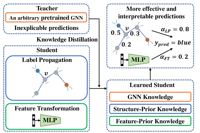
Figure 1. An overview of our knowledge distillation framework. The two simple prediction mechanisms of our student model ensure the full use of structure/feature-based prior knowledge. The knowledge in GNN teachers will be extracted and injected into the student during knowledge distillation. Thus the student can go beyond its corresponding teacher with more effective predictions.

With the success of deep learning, methods based on graph neural networks (GNNs) (Kipf and Welling, 2017; Veličković et al., 2018; Hamilton et al., 2017) have demonstrated their effectiveness in classifying node labels. Most GNN models adopt message passing strategy (Gilmer et al., 2017): each node aggregates features from its neighborhood and then a layer-wise projection function with a non-linear activation will be applied to the aggregated information. In this way, GNNs can utilize both graph structure and node feature information in their models.

However, the entanglement of graph topology, node features and projection matrices in GNNs leads to a complicated prediction mechanism and could not take full advantage of prior knowledge lying in the data. For example, the aforementioned homophily assumption adopted in label propagation methods represents structure-based prior, and has been shown to be underused (Li et al., 2019; Wang and Leskovec, 2020) in graph convolutional network (GCN) (Kipf and Welling, 2017).

As an evidence, recent studies proposed to incorporate the label propagation mechanism into GCN by adding regularizations (Wang and Leskovec, 2020) or manipulating graph filters (Li et al., 2019; Shi et al., 2020). Their experimental results show that GCN can be improved by emphasizing such structure-based prior knowledge. Nevertheless, these methods have three major drawbacks: (1) The main bodies of their models are still GNNs and thus hard to fully utilize the prior knowledge; (2) They are single models rather than frameworks, and thus not compatible with other advanced GNN architectures; (3) They ignored another important prior knowledge, i.e., feature-based prior, which means that a node’s label is purely determined by its own features.

To address these issues, we propose an effective knowledge distillation framework to inject the knowledge of an arbitrary learned GNN (teacher model) into a well-designed student model. The student model is built with two simple prediction mechanisms, i.e., label propagation and feature transformation, which naturally preserves structure-based and feature-based prior knowledge, respectively. In specific, we design the student model as a trainable combination of parameterized label propagation and feature-based $2$-layer MLP (Multi-layer Perceptron). On the other hand, it has been recognized that the knowledge of a teacher model lies in its soft predictions (Hinton et al., 2015). By simulating the soft labels predicted by a teacher model, our student model is able to further make use of the knowledge in pretrained GNNs. Consequently, the learned student model has a more interpretable prediction process and can utilize both GNN and structure/feature-based priors. An overview of our framework is shown in Fig. 1.

We conduct experiments on five public benchmark datasets and employ several popular GNN models including GCN (Kipf and Welling, 2017), GAT (Veličković et al., 2018), SAGE (Hamilton et al., 2017), APPNP (Klicpera et al., 2018), SGC (Wu et al., 2019) and a recent deep GCN model GCNII (Chen et al., 2020) as teacher models. Experimental results show that a student model is able to outperform its corresponding teacher model by $1.4\%\sim 4.7\%$ in terms of classification accuracy. It is worth noting that we also apply our framework on GLP (Li et al., 2019) which unified GCN and label propagation by manipulating graph filters. As a result, we can still gain $1.5\%\sim 2.3\%$ relative improvements, which demonstrates the potential compatibility of our framework. Furthermore, we investigate the interpretability of our student model by probing the learned balance parameters between parameterized label propagation and feature transformation as well as the learned confidence score of each node in label propagation. To conclude, the improvements are consistent and significant with better interpretability.

The contributions of this paper are summarized as follows:

$\bullet$ We propose an effective knowledge distillation framework to extract the knowledge of an arbitrary pretrained GNN model and inject it into a student model for more effective predictions.

$\bullet$ We design the student model as a trainable combination of parameterized label propagation and feature-based $2$-layer MLP. Hence the student model has a more interpretable prediction process and naturally preserves the structure/feature-based priors. Consequently, the learned student model can utilize both GNN and prior knowledge.

$\bullet$ Experimental results on five benchmark datasets with seven GNN teacher models demonstrate the effectiveness of our framework. Extensive studies by probing the learned weights in the student model also illustrate the potential interpretability of our method.

2. Related Work

This work is most relevant to graph neural network models and knowledge distillation methods.

2.1. Graph Neural Networks

The concept of GNN was proposed (Scarselli et al., 2008) before 2010 and has become a rising topic since the emergence of GCN (Kipf and Welling, 2017). During the last five years, graph neural network models have achieved promising results in many research areas (Wu et al., 2020; Zhou et al., 2018). Now we will briefly introduce some representative GNN methods in this section and employ them as our teacher models in the experiments.

As one of the most influential GNN models, Graph Convolutional Network (GCN) (Kipf and Welling, 2017) targeted on semi-supervised learning on graph-structured data through layer-wise propagation of node features. GCN can be interpreted as a variant of convolutional neural networks that operates on graphs. Graph Attention Network (GAT) (Veličković et al., 2018) further employed attention mechanism in the aggregation of neighbors’ features. SAGE (Hamilton et al., 2017) sampled and aggregated features from a node’s local neighborhood and is more space-efficient. Approximate personalized propagation of neural predictions (APPNP) (Klicpera et al., 2018) studied the relationship between GCN and PageRank, and incorporated a propagation scheme derived from personalized PageRank into graph filters. Simple Graph Convolution (SGC) (Wu et al., 2019) simplified GCN by removing non-linear activations and collapsing weight matrices between layers. Graph Convolutional Network via Initial residual and Identity mapping (GCNII) (Chen et al., 2020) was a very recent deep GCN model which alleviates the over-smoothing problem.

Recently, several works show that the performance of GNNs can be further improved by incorporating traditional prediction mechanisms, i.e., label propagation. For example, Generalized Label Propagation (GLP) (Li et al., 2019) modified graph convolutional filters to generate smooth features with graph similarity encoded. UniMP (Shi et al., 2020) fused feature aggregation and label propagation by a shared message-passing network. GCN-LPA (Wang and Leskovec, 2020) employed label propagation as regularization to assist GCN for better performances. Note that the label propagation mechanism was built with simple structure-based prior knowledge. Their improvements indicate that such prior knowledge is not fully explored in GNNs. Nevertheless, these advanced models still suffer from several drawbacks as illustrated in the Introduction section.

2.2. Knowledge Distillation

Knowledge distillation (Hinton et al., 2015) was proposed for model compression where a small light-weight student model is trained to mimic the soft predictions of a pretrained large teacher model. After the distillation, the knowledge in the teacher model will be transferred into the student model. In this way, the student model can reduce time and space complexities without losing prediction qualities. Knowledge distillation is widely used in the computer vision area, e.g., a deep convolutional neural network (CNN) will be compressed into a shallow one to accelerate the inference.

In fact, there are also a few studies combining knowledge distillation with GCN. However, their motivation and model architecture are quite different from ours. Yang et al. (Yang et al., 2020) which was proposed in the computer vision area, compressed a deep GCN with large feature maps into a shallow one with fewer parameters using a local structure preserving module. Reliable Data Distillation (RDD) (Zhang et al., 2020) trained multiple GCN students with the same architecture and then ensembled them for better performance in a manner similar to BAN (Furlanello et al., 2018). Graph Markov Neural Networks (GMNN) (Qu et al., 2019) can also be viewed as a knowledge distillation method where two GCNs with different reception sizes learn from each other. Note that both teacher and student models in these works are GCNs.

Compared with them, the goal of our framework is to extract the knowledge of GNNs and go beyond it. Our framework is very flexible and can be applied on an arbitrary GNN model besides GCN. We design a student model with simple prediction mechanisms and thus are able to benefit from both GNN and prior knowledge. As the output of our framework, the student model also has a more interpretable prediction process. In terms of training details, our framework is simpler and requires no ensembling or iterative distillations between teacher and student models for improving classification accuracies.

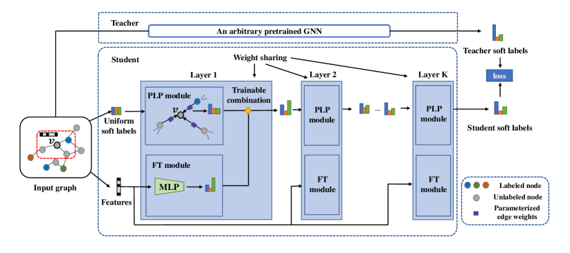
Figure 2. An illustration of the architecture of our proposed student model. Taking the center node $v$ as an example, the student model starts from node $v$’s raw features and a uniform label distribution as soft labels. Then at each layer, the soft label prediction of $v$ will be updated as a trainable combination of Parameterized Label Propagation (PLP) from $v$’s neighbors and Feature Transformation (FT) of $v$’s features. Finally, the distance between the soft label predictions of student and pretrained teacher will be minimized.

3. Methodology

In this section, we will start by formalizing the semi-supervised node classification problem and introducing the notations. Then we will present our knowledge distillation framework to extract the knowledge of GNNs. Afterwards, we will propose the architecture of our student model, which is a trainable combination of parameterized label propagation and feature-based $2$-layer MLP. Finally, we will discuss the potential interpretability of the student model and the computation complexity of our framework.

3.1. Semi-supervised Node Classification

We begin by outlining the problem of node classification. Given a connected graph $G=(V,E)$ with a subset of nodes $V_{L}\subset V$ labeled, where $V$ is the vertex set and $E$ is the edge set, node classification targets on predicting the node labels for every node $v$ in unlabeled node set $V_{U}=V\setminus V_{L}$. Each node $v\in V$ has label $y_{v}\in Y$ where $Y$ is the set of all possible labels. In addition, node features $X\in\mathbb{R}^{|V|\times d}$ are usually available in graph data and can be utilized for better classification accuracy. Each row $X_{v}\in\mathbb{R}^{d}$ of matrix $X$ denotes a $d$-dimensional feature vector of node $v$.

3.2. The Knowledge Distillation Framework

Node classification approaches including GNNs can be summarized as a black box that outputs a classifier $f$ given graph structure $G$, labeled node set $V_{L}$ and node feature $X$ as inputs. The classifier $f$ will predict the probability $f(v,y)$ that unlabeled node $v\in V_{U}$ has label $y\in Y$, where $\sum_{y^{\prime}\in Y}f(v,y’)=1$. For labeled node $v$, we set $f(v,y)=1$ if $v$ is annotated with label $y$ and $f(v,y^{\prime})=0$ for any other label $y^{\prime}$. We use $f(v)\in\mathbb{R}^{|Y|}$ to denote the probability distribution over all labels for brevity.

In this paper, the teacher model employed in our framework can be an arbitrary GNN model such as GCN (Kipf and Welling, 2017) or GAT (Veličković et al., 2018). We denote the pretrained classifier in a teacher model as $f_{GNN}$. On the other hand, we use $f_{STU;\Theta}$ to denote the student model parameterized by $\Theta$ and $f_{STU;\Theta}(v)\in\mathbb{R}^{|Y|}$ represents the predicted probability distribution of node $v$ by the student.

In knowledge distillation (Hinton et al., 2015), the student model is trained to mimic the soft label predictions of a pretrained teacher model. As a result, the knowledge lying in the teacher model will be extracted and injected into the learned student. Therefore, the optimization objective which aligns the outputs between the student model and pretrained teacher model can be formulated as

(1) $$\min_{\Theta}\sum_{v\in V}distance(f_{GNN}(v),f_{STU;\Theta}(v)),$$

where $distance(\cdot,\cdot)$ measures the distance between two predicted probability distributions. Specifically, we use Euclidean distance in this work.

3.3. The Architecture of Student Model

We hypothesize that a node’s label prediction follows two simple mechanisms: (1) label propagation from its neighboring nodes and (2) a transformation from its own features. Therefore, as shown in Fig. 2, we design our student model as a combination of these two mechanisms, i.e., a Parameterized Label Propagation (PLP) module and a Feature Transformation (FT) module, which can naturally preserve the structure/feature-based prior knowledge, respectively. After the distillation, the student will benefit from both GNN and prior knowledge with a more interpretable prediction mechanism.

In this subsection, we will first briefly review the conventional label propagation algorithm. Then we will introduce our PLP and FT modules as well as their trainable combinations.

3.3.1. Label Propagation

Label propagation (LP) (Zhu and Ghahramani, 2002) is a classical graph-based semi-supervised learning model. This model simply follows the assumption that nodes linked by an edge (or occupying the same manifold) are very likely to share the same label. Based on this hypothesis, labels will propagate from labeled nodes to unlabeled ones for predictions.

Formally, we use $f_{LP}$ to denote the final prediction of LP and $f_{LP}^{k}$ to denote the prediction of LP after $k$ iterations. In this work, we initialize the prediction of node $v$ as a one-hot label vector if $v$ is a labeled node. Otherwise, we will set a uniform label distribution for each unlabeled node $v$, which indicates that the probabilities of all classes are the same at the beginning. The initialization can be formalized as:

(2) $$f_{LP}^{0}(v)=\begin{cases}(0,...1,...0)\in\mathbb{R}^{|Y|},&\forall v\in V_{L}\\ (\frac{1}{|Y|},...\frac{1}{|Y|},...\frac{1}{|Y|})\in\mathbb{R}^{|Y|},&\forall v\in V_{U}\end{cases}$$

where $f_{LP}^{k}(v)$ is the predicted probability distribution of node $v$ at iteration $k$. In the $k+1$-th iteration, LP will update the label predictions of each unlabeled node $v\in V_{U}$ as follows:

(3) $$f_{LP}^{k+1}(v)=(1-\lambda)\frac{1}{|N_{v}|}\sum_{u\in N_{v}}f_{LP}^{k}(u)+\lambda f_{LP}^{k}(v),$$

where $N_{v}$ is the set of node $v$’s neighbors in the graph and $\lambda$ is a hyper-parameter controlling the smoothness of node updates.

Note that LP has no parameters to be trained, and thus can not fit the output of a teacher model through end-to-end training. Therefore, we retrofit LP by introducing more parameters to increase its capacity.

3.3.2. Parameterized Label Propagation Module

Now we will introduce our Parameterized Label Propagation (PLP) module by further parameterizing edge weights in LP. As shown in Eq. 3, LP model treats all neighbors of a node equally during the propagation. However, we hypothesize that the importance of different neighbors to a node should be different, which determines the propagation intensities between nodes. To be more specific, we assume that the label predictions of some nodes are more “confident” than others: e.g., a node whose predicted label is similar to most of its neighbors. Such nodes will be more likely to propagate their labels to neighbors and keep themselves unchanged.

Formally, we will assign a confidence score $c_{v}\in\mathbb{R}$ to each node $v$. During the propagation, all node $v$’s neighbors and $v$ itself will compete to propagate their labels to $v$. Following the intuition that a larger confidence score will have a larger edge weight, we rewrite the prediction update function in Eq. 3 for $f_{PLP}$ as follows:

(4) $$f_{PLP}^{k+1}(v)=\sum_{u\in N_{v}\cup\{v\}}w_{uv}f_{PLP}^{k}(u),$$

where $w_{uv}$ is the edge weight between node $u$ and $v$ computed by the following softmax function:

(5) $$w_{uv}=\frac{exp(c_{u})}{\sum_{u^{\prime}\in N_{v}\cup\{v\}}exp(c_{u^{\prime}})}.$$

Similar to LP, $f_{PLP}^{0}(v)$ is initialized as Eq. 2 and $f_{PLP}^{k}(v)$ remains the one-hot ground truth label vector for every labeled node $v\in V_{L}$ during the propagation.

Note that we can further parameterize confidence score $c_{v}$ for inductive setting as an optional choice:

(6) $$c_{v}=z^{T}X_{v},$$

where $z\in\mathbb{R}^{d}$ is a learnable parameter that projects node $v$’s feature into the confidence score.

3.3.3. Feature Transformation Module

Note that PLP module which propagates labels through edges emphasizes the structure-based prior knowledge. Thus we also introduce Feature Transformation (FT) module as a complementary prediction mechanism. The FT module predicts labels by only looking at the raw features of a node. Formally, denoting the prediction of FT module as $f_{FT}$, we apply a $2$-layer MLP followed by a softmax function to transform the features into soft label predictions:

(7) $$f_{FT}(v)=softmax(MLP(X_{v})).$$

3.3.4. A Trainable Combination

Now we will combine the PLP and FT modules as the full model of our student. In detail, we will learn a trainable parameter $\alpha_{v}\in[0,1]$ for each node $v$ to balance the predictions between PLP and FT. In other words, the prediction from FT module will be incorporated into that from PLP at each propagation step. We name the full student model as Combination of Parameterized label propagation and Feature transformation (CPF) and thus the prediction update function for each unlabeled node $v\in V_{U}$ in Eq. 4 will be rewritten as

(8) $$f_{CPF}^{k+1}(v)=\alpha_{v}\sum_{u\in N_{v}\cup\{v\}}w_{uv}f_{CPF}^{k}(u)+(1-\alpha_{v})f_{FT}(v),$$

where edge weight $w_{uv}$ and initialization $f_{CPF}^{0}(v)$ are the same with PLP module. Whether parameterizing confidence score $c_{v}$ as Eq. 6 or not will lead to inductive/transductive variants CPF-ind/CPF-tra.

3.4. The Overall Algorithm and Details

Assuming that our student model has a total of $K$ layers, the distillation objective in Eq. 1 can be detailed as:

(9) $$\min_{\Theta}\sum_{v\in V_{U}}\|f_{GNN}(v)-f_{CPF;\Theta}^{K}(v)\|_{2},$$

where $\|\cdot\|_{2}$ is the L2-norm and the parameter set $\Theta$ includes the balancing parameters between PLP and FT $\{\alpha_{v},\forall v\in V\}$, confidence parameters in PLP module $\{c_{v},\forall v\in V\}$ (or parameter $z$ for inductive setting), and the parameters of MLP in FT module $\Theta_{MLP}$. There is also an important hyper-parameter in the distillation framework: the number of propagation layers $K$. Alg. 1 shows the pseudo code of the training process.

We implement our framework based on Deep Graph Library (DGL) (Wang et al., 2019) and Pytorch (Paszke et al., 2019), and employ an Adam optimizer (Kingma and Ba, 2014) for parameter training. Dropout  (Srivastava et al., 2014) is also applied to alleviate overfitting.

Algorithm 1 The proposed knowledge distillation framework.

0:  Graph $G=(V,E)$, labeled node set $V_{L}\subset V$, unlabeled node set $V_{U}\subset V$, node features $X$ and pretrained GNN classifier $f_{GNN}$.

0:  The learned student model $f_{CPF}$.

1:  Initialize the label prediction $f_{CPF}^{0}(v)$ for each node $v$ by Eq. 2;

2:  while not converge do

3:     if inductive setting then

4:        Compute confidence score $c_{v}$ for each node $v\in V$ by Eq. 6;

5:     end if

6:     Compute edge weight $w_{uv}$ for each edge $(u,v)\in E$ by Eq. 5;

7:     for all node $v\in V_{U}$ do

8:        Compute the prediction of FT module $f_{FT}(v)$ by Eq. 7;

9:        for k=1,2…K do

10:           Update the prediction after $k$ layers $f_{CPF}^{k}(v)$ by Eq. 8;

11:        end for

12:     end for

13:     Update parameters by optimizing Eq. 9;

14:  end while

3.5. Discussions on Interpretability and Complexity

In this subsection, we will discuss the interpretability of the learned student model and the complexity of our algorithm.

After the knowledge distillation, our student model CPF will predict the label of a specific node $v$ as a weighted average between the predictions of label propagation and feature-based MLP. The balance parameter $\alpha_{v}$ indicates whether structure-based LP or feature-based MLP is more important for node $v$’s prediction. LP mechanism is almost transparent and we can easily find out node $v$ is influenced by which neighbor to what extent at each iteration. On the other hand, the understanding of feature-based MLP can be derived by existing works (Ribeiro et al., 2016) or directly looking at the gradients of different features. Therefore, the learned student model has better interpretability than GNN teachers.

The time complexity of each iteration (line 3 to 13 in Alg. 1) and the space complexity of our algorithm are both $O(|E|+d|V|)$, which is linear to the scale of datasets. In fact, the operations can be easily implemented in matrix form and the training process can be finished in seconds on real-world benchmark datasets with a single GPU device. Therefore, our proposed knowledge distillation framework is very time/space-efficient.

4. Experiments

In this section, we will start by introducing the datasets and teacher models used in our experiments. Then we will detail the experimental settings of teacher models and student variants. Afterwards, we will present quantitative results on evaluating semi-supervised node classification. We also conduct experiments under different numbers of propagation layers and training ratios to illustrate the robustness of our algorithm. Finally, we will present qualitative case studies and visualizations for better understandings of the learned parameters in our student model CPF.

4.1. Datasets

Table 1. Dataset statistics.

Dataset	# Nodes	# Edges	# Features	# Classes
Cora	2,485	5,069	1,433	7
Citeseer	2,110	3,668	3,703	6
Pubmed	19,717	44,324	500	3
A-Computers	13,381	245,778	767	10
A-Photo	7,487	119,043	745	8

Table 2. Classification accuracies with teacher models as GCN (Kipf and Welling, 2017) and GAT (Veličković et al., 2018).

Datasets	Teacher	Student variants				+Impv.	Teacher	Student variants				+Impv.
	GCN	PLP	FT	CPF-ind	CPF-tra		GAT	PLP	FT	CPF-ind	CPF-tra
Cora	0.8244	0.7522	0.8253	0.8576	0.8567	4.0%	0.8389	0.7578	0.8426	0.8576	0.8590	2.4%
Citeseer	0.7110	0.6602	0.7055	0.7619	0.7652	7.6%	0.7276	0.6624	0.7591	0.7657	0.7691	5.7%
Pubmed	0.7804	0.6471	0.7964	0.8080	0.8104	3.8%	0.7702	0.6848	0.7896	0.8011	0.8040	4.4%
A-Computers	0.8318	0.7584	0.8356	0.8443	0.8443	1.5%	0.8107	0.7605	0.8135	0.8190	0.8148	1.0%
A-Photo	0.9072	0.8499	0.9265	0.9317	0.9248	2.7%	0.8987	0.8496	0.9190	0.9221	0.9199	2.6%

Table 3. Classification accuracies with teacher models as APPNP (Klicpera et al., 2018) and SAGE (Hamilton et al., 2017).

Datasets	Teacher	Student variants				+Impv.	Teacher	Student variants				+Impv.
	APPNP	PLP	FT	CPF-ind	CPF-tra		SAGE	PLP	FT	CPF-ind	CPF-tra
Cora	0.8398	0.7251	0.8379	0.8581	0.8562	2.2%	0.8178	0.7663	0.8201	0.8473	0.8454	3.6%
Citeseer	0.7547	0.6812	0.7580	0.7646	0.7635	1.3%	0.7171	0.6641	0.7425	0.7497	0.7575	5.6%
Pubmed	0.7950	0.6866	0.8102	0.8058	0.8081	1.6%	0.7736	0.6829	0.7717	0.7948	0.8062	4.2%
A-Computers	0.8236	0.7516	0.8176	0.8279	0.8211	0.5%	0.7760	0.7590	0.7912	0.7971	0.8199	5.7%
A-Photo	0.9148	0.8469	0.9241	0.9273	0.9272	1.4%	0.8863	0.8366	0.9153	0.9268	0.9248	4.6%

We use five public benchmark datasets for experiments and the statistics of the datasets are shown in Table 1. As previous works (Shchur et al., 2018; Klicpera et al., 2019; Sun et al., 2020) did, we only consider the largest connected component and regard the edges as undirected. The details about the datasets are as follows:

• Cora (Sen et al., 2008) is a benchmark citation dataset composed of machine learning papers, where each node represents a document with a sparse bag-of-words feature vector. Edges represent citations between documents, and labels specify the research field of each paper.

• Citeseer (Sen et al., 2008) is another benchmark citation dataset of computer science publications, holding similar configuration to Cora. Citeseer dataset has the largest number of features among all five datasets used in this paper.

• Pubmed (Namata et al., 2012) is also a citation dataset, consisting of articles related to diabetes in the PubMed database. The node features are TF/IDF weighted word frequency, and the label indicates the type of diabetes discussed in this article.

• A-Computers and A-Photo (Shchur et al., 2018) are extracted from Amazon co-purchase graph, where nodes represent products, edges represent whether two products are frequently co-purchased or not, features represent product reviews encoded by bag-of-words, and labels are predefined product categories.

Following the experimental settings in previous work (Shchur et al., 2018), we randomly sample $20$ nodes from each class as labeled nodes, $30$ nodes for validation and all other nodes for test.

4.2. Teacher Models and Settings

For a thorough comparison, we consider seven GNN models as teacher models in our knowledge distillation framework:

• GCN (Kipf and Welling, 2017) is a classic semi-supervised model which learns node representations by defining convolution operators on graph-structured data. GCN is sensitive to the number of layers and we employ the most widely-used $2$-layer setting in this work.

• GAT (Veličković et al., 2018) improves GCN by incorporating attention mechanism which assigns different weights to each neighbor of a node. We use a $2$-layer GAT with $8$ attention heads as our teacher model.

• APPNP (Klicpera et al., 2018) improves GCN by balancing the preservation of local information and the use of a wide range of neighbor information. We employ $2$ layers and $10$ power iteration steps for APPNP.

• SAGE (Hamilton et al., 2017) learns node embeddings by sampling and aggregating information from a node’s local neighborhood. We employ the SAGE-GCN variant as a teacher model.

• SGC (Wu et al., 2019) reduces the extra complexity of GCN by removing the non-linearity between GCN layers and compressing the weight matrices. Similar to GCN, we also use a $2$-layer setting.

• GCNII (Chen et al., 2020) is a deep model which uses initial residual and identity mapping to avoid oversmoothing of GCN model. Here we use $16$ layers GCNII as a teacher.

• GLP (Li et al., 2019) is a label-efficient model which combines label propagation with graph convolution operations by a graph filtering framework. GLP has two model variants: GLP-RNM and GLP-AR, and we use the better one for each dataset as our teacher.

The detailed training settings of teacher models are listed in Appendix A.

4.3. Student Variants and Experimental Settings

For each dataset and teacher model, we test the following student variants:

• PLP: The student variant with only the Parameterized Label Propagation (PLP) mechanism;

• FT: The student variant with only the Feature Transformation (FT) mechanism;

• CPF-ind: The full model CPF with inductive setting;

• CPF-tra: The full model CPF with transductive setting.

We randomly initialize the parameters and employ early stopping with a patience of $50$, i.e., we will stop training if the classification accuracy on validation set does not increase for $50$ epochs. For hyper-parameter tuning, we conduct heuristic search by exploring # layers $K\in\{5,6,7,8,9,10\}$, hidden size in MLP $d_{MLP}\in\{8,16,32,64\}$, dropout rate $dr\in\{0.2,0.5,0.8\}$, learning rate and weight decay of Adam optimizer $lr\in\{0.001,0.005,0.01\},wd\in\{0.0005,0.001,0.01\}$.

Table 4. Classification accuracies with teacher models as SGC (Wu et al., 2019) and GCNII (Chen et al., 2020).

Datasets	Teacher	Student variants				+Impv.	Teacher	Student variants				+Impv.
	SGC	PLP	FT	CPF-ind	CPF-tra		GCNII	PLP	FT	CPF-ind	CPF-tra
Cora	0.8052	0.7513	0.8173	0.8454	0.8487	5.4%	0.8384	0.7382	0.8431	0.8581	0.8590	2.5%
Citeseer	0.7133	0.6735	0.7331	0.7470	0.7530	5.6%	0.7376	0.6724	0.7564	0.7635	0.7569	3.5%
Pubmed	0.7892	0.6018	0.8098	0.7972	0.8204	4.0%	0.7971	0.6913	0.7984	0.7928	0.8024	0.7%
A-Computers	0.8248	0.7579	0.8391	0.8367	0.8407	1.9%	0.8325	0.7628	0.8411	0.8467	0.8447	1.7%
A-Photo	0.9063	0.8318	0.9303	0.9397	0.9347	3.7%	0.9230	0.8401	0.9263	0.9352	0.9300	1.3%

Table 5. Classification accuracies with teacher model as GLP (Li et al., 2019).

Datasets	Teacher	Student variants				+Impv.
	GLP	PLP	FT	CPF-ind	CPF-tra
Cora	0.8365	0.7616	0.8314	0.8557	0.8539	2.3%
Citeseer	0.7536	0.6630	0.7597	0.7696	0.7696	2.1%
Pubmed	0.8088	0.6215	0.7842	0.8133	0.8210	1.5%

4.4. Analysis of Classification Results

Experimental results on five datasets with seven GNN teachers and four student variants are presented in Table 2,  3,  4 and  5. We have the following observations:

• The proposed knowledge distillation framework accompanying with the full architecture of student model CPF-ind and CPF-tra, is able to improve the performance of the corresponding teacher model consistently and significantly. For example, the classification accuracy of GCN on Cora dataset is improved from $0.8244$ to $0.8576$. This is because the knowledge of GNN teachers can be extracted and injected into our student model which also benefits from structure/feature-based prior knowledge introduced by its simple prediction mechanism. This observation demonstrates our motivation and the effectiveness of our framework.

• Note that the teacher model Generalized Label Propagation (GLP) (Li et al., 2019) has already incorporated the label propagation mechanism in their graph filters. As shown in Table 5, we can still gain $1.5\%\sim 2.3\%$ relative improvements by applying our knowledge distillation framework, which demonstrates the potential compatibility of our algorithm.

• Among the four student variants, the full model CPF-ind and CPF-tra always perform best (except APPNP teacher on Pubmed dataset) and give competitive results. Thus both structure-based PLP and feature-based FT modules will contribute to the overall improvements. PLP itself performs worst because PLP which has few parameters to learn has a small model capacity and can not fit the soft predictions of teacher models.

• The average relative improvements of the seven teachers
  GCN/GAT/APPNP/SAGE/SGC/GCNII/GLP are 3.9/3.2/1.4/ 4.7/4.1/1.9/2.0%, respectively. The improvement over APPNP is the smallest. A possible reason is that APPNP preserves a node’s own features during the message passing and thus also utilizes the feature-based prior as our FT module does.

• The average relative improvements on the five datasets Cora/
  Citeseer/Pubmed/A-Computers/A-Photo are 2.9/4.2/2.7/2.1/ 2.7%, respectively. Citeseer dataset benefits most from our knowledge distillation framework. A possible reason is that Citeseer has the largest number of features and thus the student model also has more trainable parameters to increase its capacity.

4.5. Analysis of Different Numbers of Propagation Layers

In this subsection, we will investigate the influence of a key hyper-parameter in the architecture of our student model CPF, i.e., the number of propagation layers $K$. In fact, popular GNN models such as GCN and GAT are very sensitive to the number of layers. A larger number of layers will cause the over-smoothing issue and significantly harm the model performance. Hence we conduct experiments on Cora dataset for further analysis of this hyper-parameter.

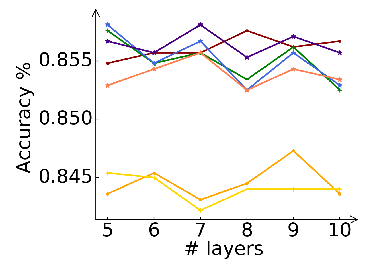
(a) The CPF-ind student.

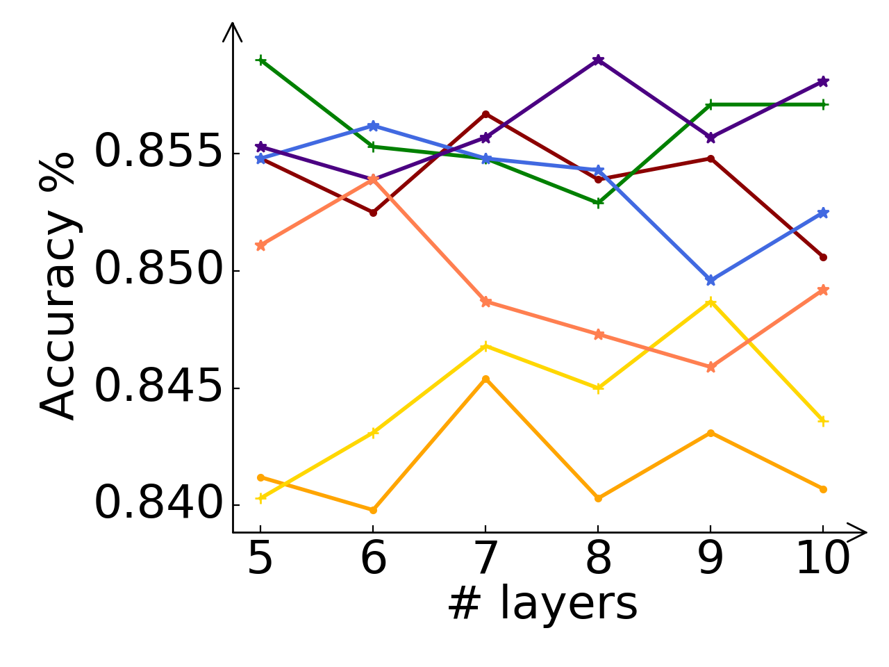
(b) The CPF-tra student.

Figure 3. Classification accuracies of CPF-ind and CPF-tra with different numbers of propagation layers on Cora dataset. The legends indicate the teacher model by which a student is guided.

Fig. 3 shows the classification results of student CPF-ind and CPF-tra with different numbers of propagation layers $K\in\{5,6,7,8,9,10\}$. We can see that the gaps among different $K$ are relatively small: For each teacher, we compute the gap between the best and worst performed accuracies of its corresponding student and the maximum gaps are $0.56\%$ and $0.84\%$ for CPF-ind and CPF-tra, respectively. Moreover, the accuracy of CPF under the worst choice of $K\in\{5,6,7,8,9,10\}$ has already outperformed the corresponding teacher. Therefore, the gains from our framework are very robust when the number of propagation layers $K$ varies within a reasonable range.

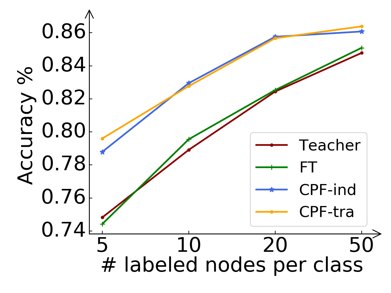
(a) GCN

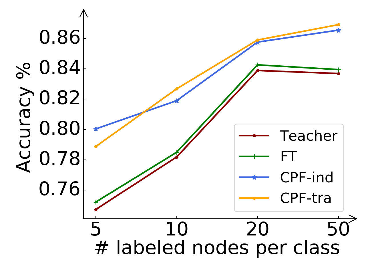
(b) GAT

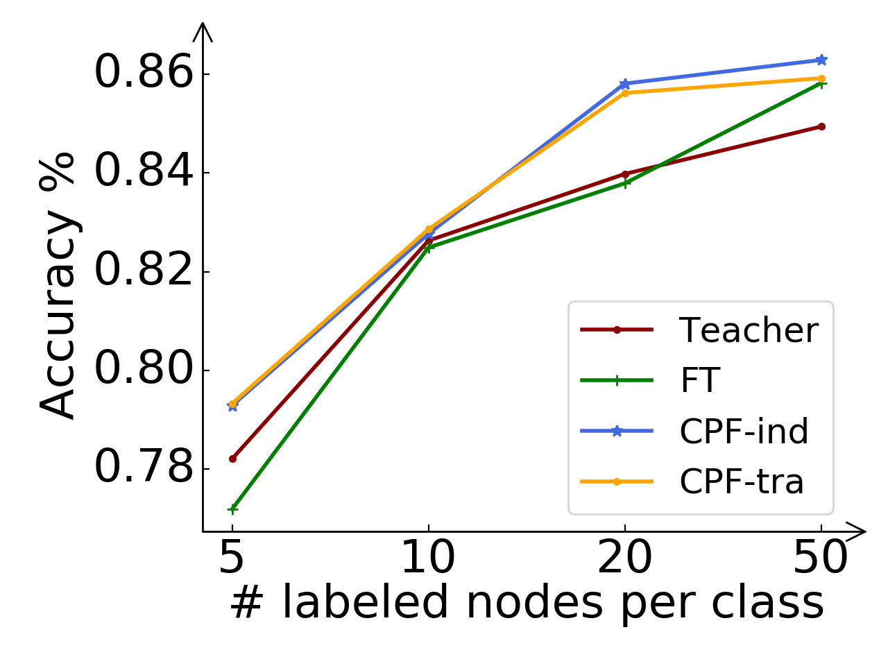
(c) APPNP

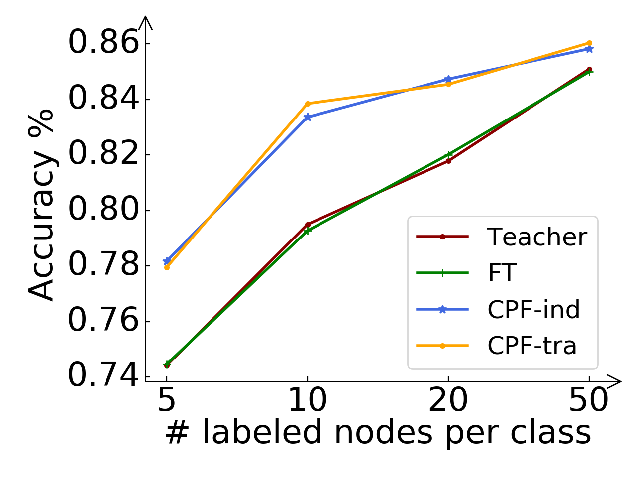
(d) SAGE

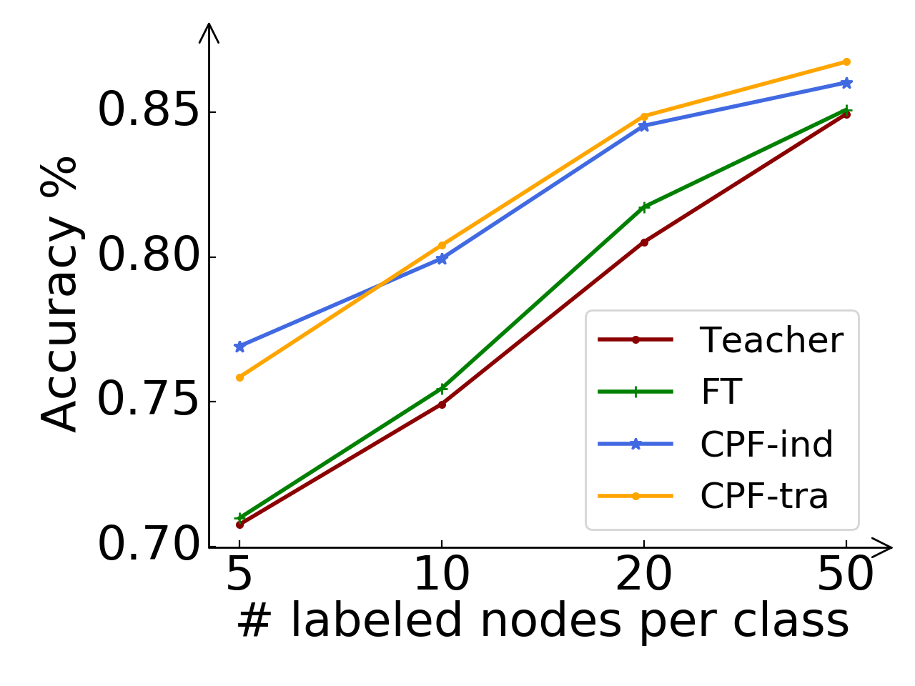
(e) SGC

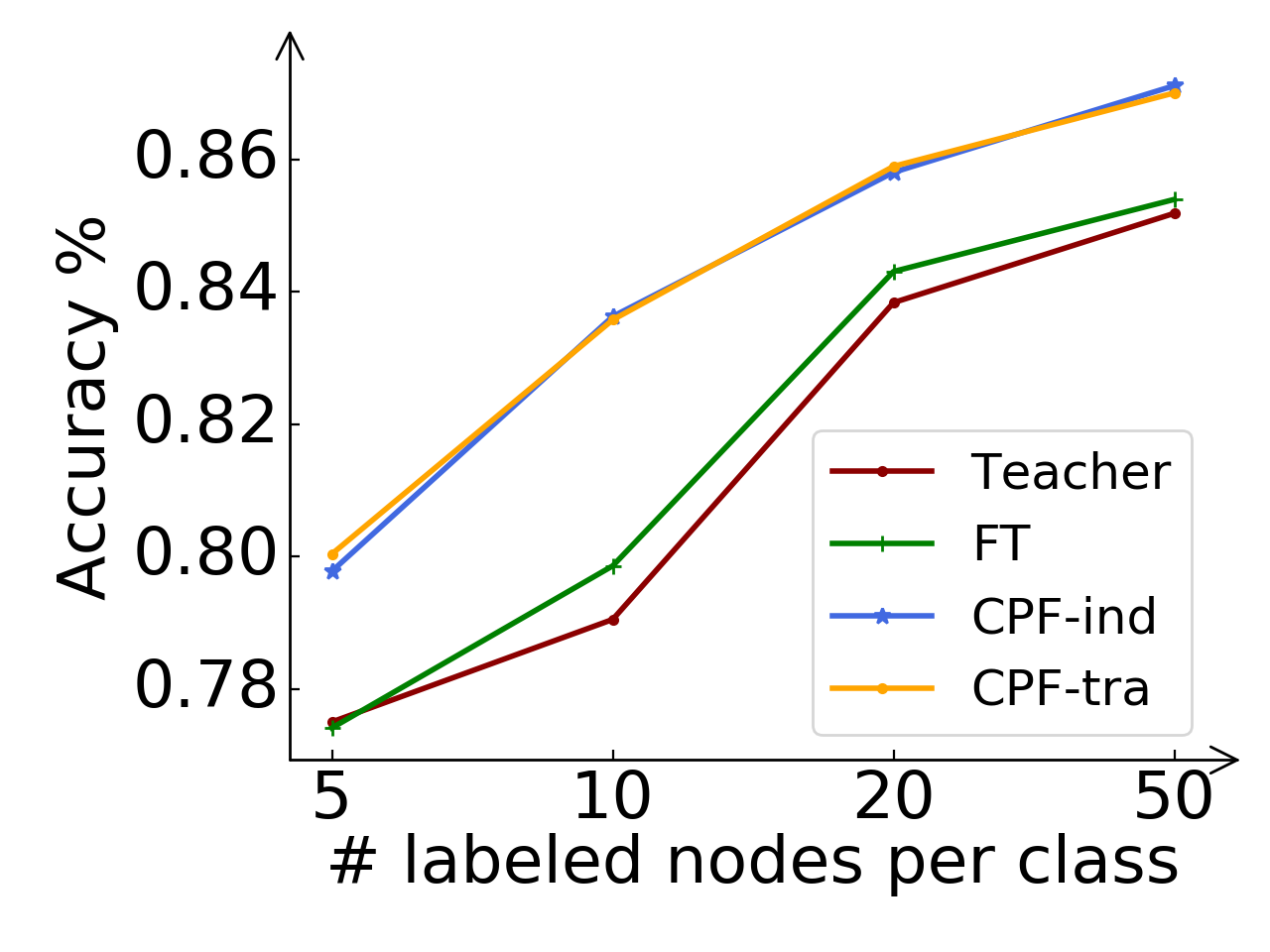
(f) GCNII

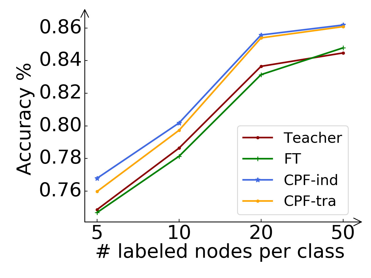
(g) GLP

Figure 4. Classification accuracies under different numbers of labeled nodes on Cora dataset. The subcaptions indicate the corresponding teacher models.

Besides changing the number of propagation layers, another model variant we test is replacing the 2-layer MLP in feature transformation module with a single-layer linear regression, which can also improve the performance with a smaller ratio (the average improvements over the seven teachers are $0.3\%\sim 2.3\%$). Linear regression may have better interpretability, but at the cost of weaker performance, which can be seen as a trade-off.

4.6. Analysis of Different Training Ratios

To further demonstrate the effectiveness of our framework, we conduct additional experiments under different training ratios. In specific, we take Cora dataset as an example and vary the number of labeled nodes per class from $5$ to $50$. Experimental results are presented in Fig. 4. Note that we omit the results of PLP since its performance is poor and can not be fit into the figures.

We can see that the learned CPF-ind and CPF-tra students consistently outperform the pretrained GNN teachers under different numbers of labeled nodes per class, which illustrates the robustness of our framework. FT module, however, has enough model capacity to overfit the predictions of a teacher but gains no further improvements. Therefore, as a complementary prediction mechanism, the PLP module is also very important in our framework.

Another observation is that the students’ improvements over corresponding teacher models are more significant for the few-shot setting, i.e., only $5$ nodes are labeled for each class. As evidence, the relative improvements on classification accuracy are $4.9/4.5/3.2/2.1\%$ on average for $5/10/20/50$ labeled nodes per class. Thus our algorithm also has the ability to handle the few-shot setting which is an important research problem in semi-supervised learning.

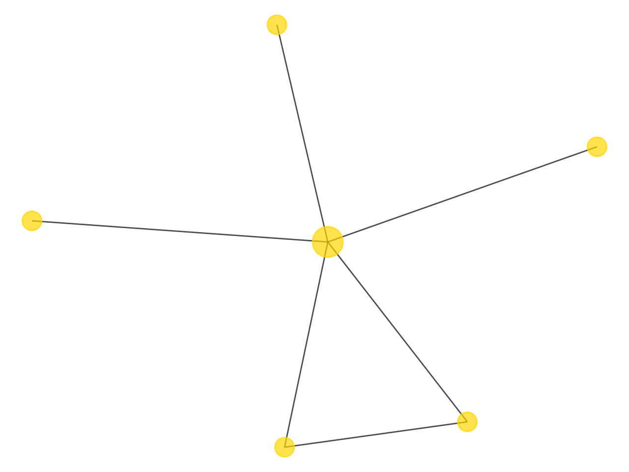
(a) Large-$\alpha_{v}$-GCN (id 1812)

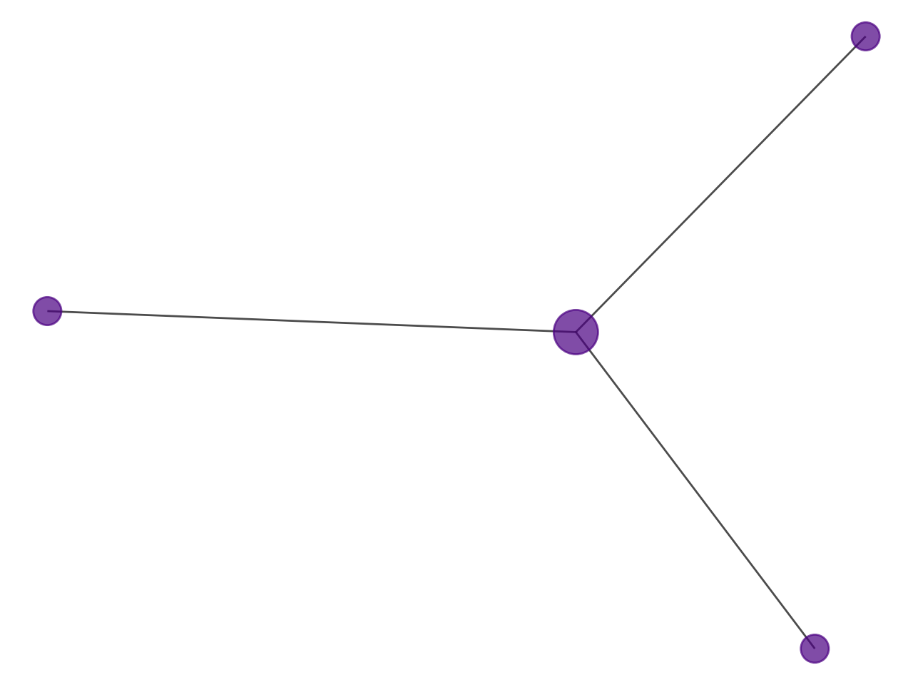
(b) Large-$\alpha_{v}$-GAT (id 1720)

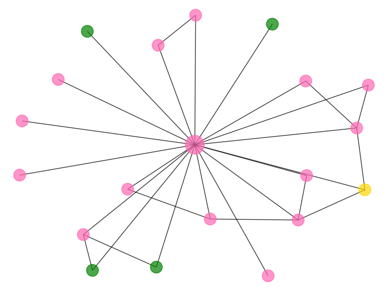
(c) Small-$\alpha_{v}$-GCN (id 2381)

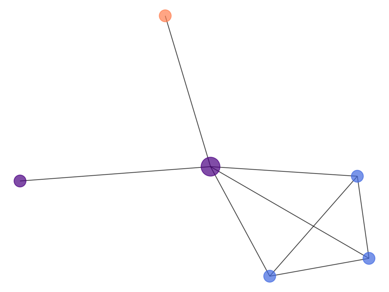
(d) Small-$\alpha_{v}$-GAT (id 1298)

Figure 5. Case studies of balance parameter $\alpha_{v}$ for interpretability analysis. Here the subcaption indicates the node is selected by large/small $\alpha_{v}$ value with GCN/GAT as teachers.

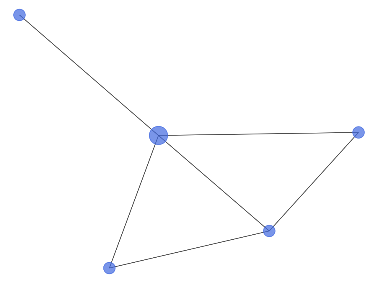
(a) Large-$c_{v}$-GCN (id 1828)

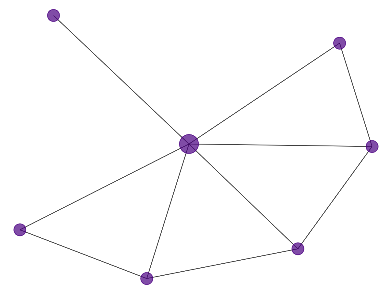
(b) Large-$c_{v}$-GAT (id 1450)

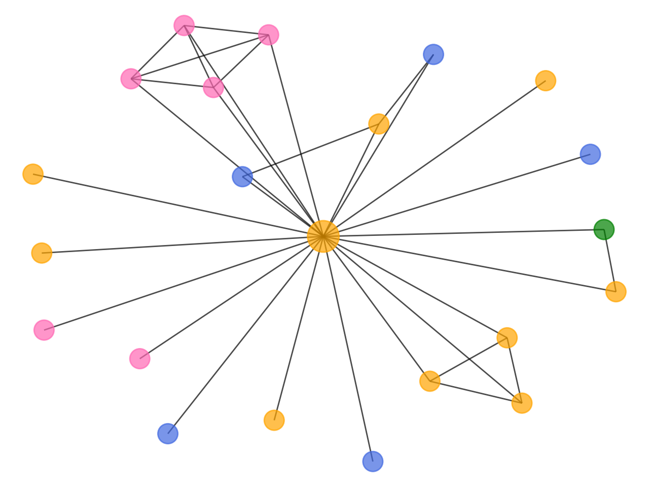
(c) Small-$c_{v}$-GCN (id 1238)

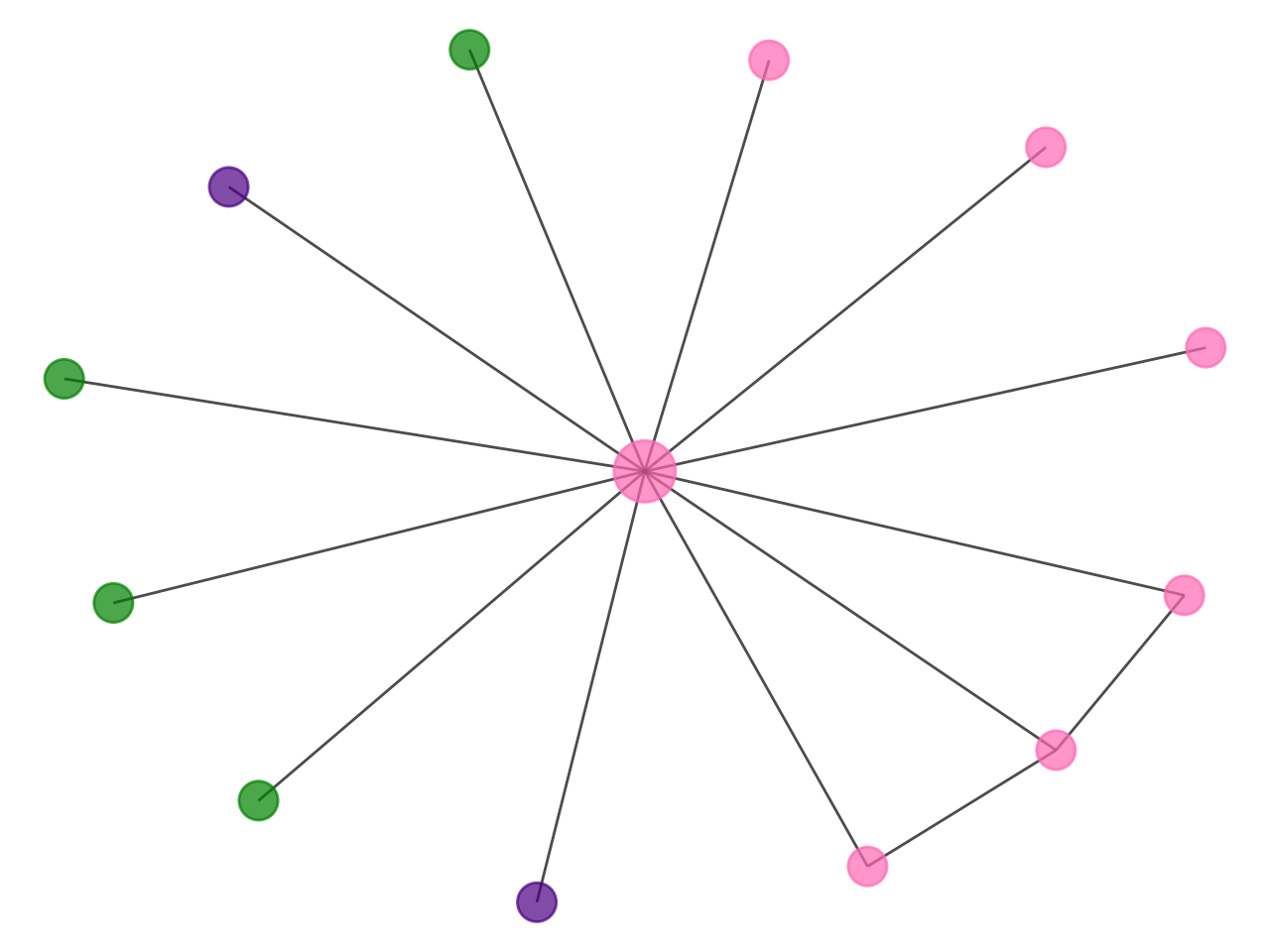
(d) Small-$c_{v}$-GAT (id 1160)

Figure 6. Case studies of confidence score $c_{v}$ for interpretability analysis. Here the subcaption indicates the node is selected by large/small $c_{v}$ value with GCN/GAT as teachers.

4.7. Analysis of Interpretability

Now we will analyze the potential interpretability of the learned student model CPF. Specifically, we will probe into the learned balance parameter $\alpha_{v}$ between PLP and FT, as well as the confidence score $c_{v}$ of each node. Our goal is to figure out what kind of nodes has the largest/smallest values of $\alpha_{v}$ and $c_{v}$. We use the CPF-ind student guided by GCN or GAT teachers on Cora dataset for illustration in this subsection.

Balance parameter $\alpha_{v}$. Recall that the balance parameter $\alpha_{v}$ indicates whether structure-based LP or feature-based MLP contributes more for node $v$’s prediction. As shown in Fig. 5, we analyze the top-10 nodes with the largest/smallest $\alpha_{v}$ and select four representative nodes for case study. We plot the 1-hop neighborhood of each node and use different colors to indicate different predicted labels. We find that a node with a larger $\alpha_{v}$ will be more likely to have the same predicted neighbors. In contrast, a node with a smaller $\alpha_{v}$ will probably have more neighbors with different predicted labels. This observation matches our intuition that the prediction of a node will be confused if it has many neighbors with various predicted labels and thus can not benefit much from label propagation.

Confidence score $c_{v}$. On the other hand, a node with a larger confidence score $c_{v}$ in our student architecture will have larger edge weights to propagate its labels to neighbors and keep itself unchanged. Similarly, as shown in Fig. 6, we also investigate the top-10 nodes with the largest/smallest confidence score $c_{v}$ and select four representative nodes for case study. We can see that nodes with high confidences will also have a relatively small degree and the same predicted neighbors. In contrast, nodes with low confidences $c_{v}$ will have an even more diverse neighborhood than nodes with small $\alpha_{v}$. Intuitively, a diverse neighborhood of a node will lead to lower confidence to propagate its labels. This finding validates our motivation for modeling node confidences.

5. Conclusion

In this paper, we propose an effective knowledge distillation framework which can extract the knowledge of an arbitrary pretrained GNN (teacher model) and inject it into a well-designed student model. The student model CPF is built as a trainable combination of two simple prediction mechanisms: label propagation and feature transformation which emphasize structure-based and feature-based prior knowledge, respectively. After the distillation, the learned student is able to take advantage of both prior and GNN knowledge and thus go beyond the GNN teacher. Experimental results on five benchmark datasets show that our framework can improve the classification accuracies of all seven GNN teacher models consistently and significantly with a more interpretable prediction process. Additional experiments on different numbers of training ratios and propagation layers demonstrate the robustness of our algorithm. We also present case studies to understand the learned balance parameters and confidence scores in our student architecture.

For future work, we will explore the adoption of our framework for other graph-based applications besides semi-supervised node classification. For example, the unsupervised node clustering task would be interesting since the label propagation scheme can not be applied without labels. Another direction is to refine our framework by encouraging the teacher and student models to learn from each other for better performances.

6. Acknowledgment

This work is supported by the National Natural Science Foundation of China (No. U20B2045, 62002029, 61772082, 61702296), the Fundamental Research Funds for the Central Universities 2020RC23, and the National Key Research and Development Program of China (2018YFB1402600).

Appendix A Details for Reproducibility

In the appendix, we provide more details of experimental settings of teacher models for reproducibility.

The training settings of 5 classical GNNs come from the paper (Shchur et al., 2018). For the two recent ones (GCNII and GLP), we follow the settings in their original papers. The details are as follows:

• GCN (Kipf and Welling, 2017): we use 64 as hidden-layer size, 0.01 as learning rate, 0.8 as dropout probability and 0.001 as learning rate decay.

• GAT (Veličković et al., 2018): we use 64 as hidden-layer size, 0.01 as learning rate, 0.6 as dropout probability, 0.3 as attention dropout probability, and 0.01 as learning rate decay.

• APPNP (Klicpera et al., 2018): we use 64 as hidden-layer size, 0.01 as learning rate, 0.5 as dropout probability and 0.01 as learning rate decay.

• SAGE (Hamilton et al., 2017): we use 128 as hidden-layer size, 0.01 as learning rate, 5 as sample number, 256 as batch size and 0.0005 as learning rate decay.

• SGC (Wu et al., 2019): we use 0.1 as learning rate and 0.001 as learning rate decay.

• GCNII (Chen et al., 2020): we use 16 as layer number, 64 as hidden-layer size, 0.01 as learning rate, 0.6 as dropout probability, 256 as batch size and 0.1/0.0005 as learning rate decays.

• GLP (Li et al., 2019): we use 16 as hidden-layer size, 0.01 as learning rate, 0.5 as dropout probability, 0.0005 as learning rate decay, k=2 for rnm setting and alpha=10 for ar setting.

References

- (1)
- Aggarwal and Zhai (2012) Charu C Aggarwal and ChengXiang Zhai. 2012. A survey of text classification algorithms. In Mining text data. Springer, 163–222.
- Altenburger and Ugander (2017) Kristen M Altenburger and Johan Ugander. 2017. Bias and variance in the social structure of gender. arXiv preprint arXiv:1705.04774 (2017).
- Bhagat et al. (2011) Smriti Bhagat, Graham Cormode, and S Muthukrishnan. 2011. Node classification in social networks. In Social network data analytics. Springer, 115–148.
- Chen et al. (2020) Ming Chen, Zhewei Wei, Zengfeng Huang, Bolin Ding, and Yaliang Li. 2020. Simple and deep graph convolutional networks. arXiv preprint arXiv:2007.02133 (2020).
- Furlanello et al. (2018) Tommaso Furlanello, Zachary Lipton, Michael Tschannen, Laurent Itti, and Anima Anandkumar. 2018. Born Again Neural Networks. In International Conference on Machine Learning. 1607–1616.
- Gilmer et al. (2017) Justin Gilmer, Samuel S Schoenholz, Patrick F Riley, Oriol Vinyals, and George E Dahl. 2017. Neural message passing for Quantum chemistry. In Proceedings of the 34th International Conference on Machine Learning-Volume 70. 1263–1272.
- Hamilton et al. (2017) Will Hamilton, Zhitao Ying, and Jure Leskovec. 2017. Inductive representation learning on large graphs. In Advances in neural information processing systems. 1024–1034.
- Hinton et al. (2015) Geoffrey Hinton, Oriol Vinyals, and Jeff Dean. 2015. Distilling the knowledge in a neural network. arXiv preprint arXiv:1503.02531 (2015).
- Joachims (2003) Thorsten Joachims. 2003. Transductive learning via spectral graph partitioning. In Proceedings of the Twentieth International Conference on International Conference on Machine Learning. 290–297.
- Kingma and Ba (2014) Diederik P Kingma and Jimmy Ba. 2014. Adam: A method for stochastic optimization. arXiv preprint arXiv:1412.6980 (2014).
- Kipf and Welling (2017) Thomas N Kipf and Max Welling. 2017. Semi-supervised classification with graph convolutional networks. In 5th International Conference on Learning Representations.
- Klicpera et al. (2018) Johannes Klicpera, Aleksandar Bojchevski, and Stephan Günnemann. 2018. Predict then Propagate: Graph Neural Networks meet Personalized PageRank. In International Conference on Learning Representations.
- Klicpera et al. (2019) Johannes Klicpera, Stefan Weißenberger, and Stephan Günnemann. 2019. Diffusion improves graph learning. In Advances in Neural Information Processing Systems. 13354–13366.
- Li et al. (2019) Qimai Li, Xiao-Ming Wu, Han Liu, Xiaotong Zhang, and Zhichao Guan. 2019. Label efficient semi-supervised learning via graph filtering. In Proceedings of the IEEE Conference on Computer Vision and Pattern Recognition. 9582–9591.
- Li et al. (2014) Rui Li, Chi Wang, and Kevin Chen-Chuan Chang. 2014. User profiling in an ego network: co-profiling attributes and relationships. In Proceedings of the 23rd international conference on World wide web. 819–830.
- McPherson et al. (2001) Miller McPherson, Lynn Smith-Lovin, and James M Cook. 2001. Birds of a feather: Homophily in social networks. Annual review of sociology 27, 1 (2001), 415–444.
- Namata et al. (2012) Galileo Namata, Ben London, Lise Getoor, Bert Huang, and UMD EDU. 2012. Query-driven active surveying for collective classification. In 10th International Workshop on Mining and Learning with Graphs, Vol. 8.
- Paszke et al. (2019) Adam Paszke, Sam Gross, Francisco Massa, Adam Lerer, James Bradbury, Gregory Chanan, Trevor Killeen, Zeming Lin, Natalia Gimelshein, Luca Antiga, et al. 2019. Pytorch: An imperative style, high-performance deep learning library. In Advances in neural information processing systems. 8026–8037.
- Qu et al. (2019) Meng Qu, Yoshua Bengio, and Jian Tang. 2019. GMNN: Graph Markov Neural Networks. In International Conference on Machine Learning. 5241–5250.
- Ribeiro et al. (2016) Marco Tulio Ribeiro, Sameer Singh, and Carlos Guestrin. 2016. ” Why should I trust you?” Explaining the predictions of any classifier. In Proceedings of the 22nd ACM SIGKDD international conference on knowledge discovery and data mining. 1135–1144.
- Scarselli et al. (2008) Franco Scarselli, Marco Gori, Ah Chung Tsoi, Markus Hagenbuchner, and Gabriele Monfardini. 2008. The graph neural network model. IEEE Transactions on Neural Networks 20, 1 (2008), 61–80.
- Sen et al. (2008) Prithviraj Sen, Galileo Namata, Mustafa Bilgic, Lise Getoor, Brian Galligher, and Tina Eliassi-Rad. 2008. Collective classification in network data. AI magazine 29, 3 (2008), 93–93.
- Shchur et al. (2018) Oleksandr Shchur, Maximilian Mumme, Aleksandar Bojchevski, and Stephan Günnemann. 2018. Pitfalls of graph neural network evaluation. arXiv preprint arXiv:1811.05868 (2018).
- Shi et al. (2020) Yunsheng Shi, Zhengjie Huang, Shikun Feng, and Yu Sun. 2020. Masked Label Prediction: Unified Massage Passing Model for Semi-Supervised Classification. arXiv preprint arXiv:2009.03509 (2020).
- Srivastava et al. (2014) Nitish Srivastava, Geoffrey Hinton, Alex Krizhevsky, Ilya Sutskever, and Ruslan Salakhutdinov. 2014. Dropout: a simple way to prevent neural networks from overfitting. The journal of machine learning research 15, 1 (2014), 1929–1958.
- Sun et al. (2020) Ke Sun, Zhouchen Lin, and Zhanxing Zhu. 2020. Multi-Stage Self-Supervised Learning for Graph Convolutional Networks on Graphs with Few Labeled Nodes. In Thirty-Fourth AAAI Conference on Artificial Intelligence.
- Szummer and Jaakkola (2002) Martin Szummer and Tommi Jaakkola. 2002. Partially labeled classification with Markov random walks. In Advances in neural information processing systems. 945–952.
- Tang and Liu (2009) Lei Tang and Huan Liu. 2009. Scalable learning of collective behavior based on sparse social dimensions. In Proceedings of the 18th ACM conference on Information and knowledge management. 1107–1116.
- Veličković et al. (2018) Petar Veličković, Guillem Cucurull, Arantxa Casanova, Adriana Romero, Pietro Liò, and Yoshua Bengio. 2018. Graph Attention Networks. In International Conference on Learning Representations.
- Wang and Leskovec (2020) Hongwei Wang and Jure Leskovec. 2020. Unifying graph convolutional neural networks and label propagation. arXiv preprint arXiv:2002.06755 (2020).
- Wang et al. (2019) Minjie Wang, Lingfan Yu, Da Zheng, Quan Gan, Yu Gai, Zihao Ye, Mufei Li, Jinjing Zhou, Qi Huang, Chao Ma, et al. 2019. Deep graph library: Towards efficient and scalable deep learning on graphs. arXiv preprint arXiv:1909.01315 (2019).
- Wu et al. (2019) Felix Wu, Amauri Souza, Tianyi Zhang, Christopher Fifty, Tao Yu, and Kilian Weinberger. 2019. Simplifying Graph Convolutional Networks. In International Conference on Machine Learning. 6861–6871.
- Wu et al. (2020) Zonghan Wu, Shirui Pan, Fengwen Chen, Guodong Long, Chengqi Zhang, and S Yu Philip. 2020. A comprehensive survey on graph neural networks. IEEE Transactions on Neural Networks and Learning Systems (2020).
- Yang et al. (2020) Yiding Yang, Jiayan Qiu, Mingli Song, Dacheng Tao, and Xinchao Wang. 2020. Distilling Knowledge From Graph Convolutional Networks. In Proceedings of the IEEE/CVF Conference on Computer Vision and Pattern Recognition. 7074–7083.
- Zhang et al. (2020) Wentao Zhang, Xupeng Miao, Yingxia Shao, Jiawei Jiang, Lei Chen, Olivier Ruas, and Bin Cui. 2020. Reliable Data Distillation on Graph Convolutional Network. In Proceedings of the 2020 ACM SIGMOD International Conference on Management of Data. 1399–1414.
- Zhou et al. (2004) Dengyong Zhou, Olivier Bousquet, Thomas N Lal, Jason Weston, and Bernhard Schölkopf. 2004. Learning with local and global consistency. In Advances in neural information processing systems. 321–328.
- Zhou et al. (2018) Jie Zhou, Ganqu Cui, Zhengyan Zhang, Cheng Yang, Zhiyuan Liu, Lifeng Wang, Changcheng Li, and Maosong Sun. 2018. Graph neural networks: A review of methods and applications. arXiv preprint arXiv:1812.08434 (2018).
- Zhu and Ghahramani (2002) Xiaojin Zhu and Zoubin Ghahramani. 2002. Learning from labeled and unlabeled data with label propagation. Technical Report CMU-CALD-02-107, Carnegie Mellon University (2002).
- Zhu et al. (2003) Xiaojin Zhu, Zoubin Ghahramani, and John Lafferty. 2003. Semi-supervised learning using Gaussian fields and harmonic functions. In Proceedings of the Twentieth International Conference on International Conference on Machine Learning. 912–919.