\corres

*Frédéric Ouimet

\presentaddress\orgdiv

Department of Mathematics and Statistics, \orgnameMcGill University, \orgaddress\stateQuebec, \countryCanada

A multivariate normal approximation for the Dirichlet density and some applications

Frédéric Ouimet \orgdivDivision of Physics, Mathematics and Astronomy, \orgnameCalifornia Institute of Technology, \orgaddress\stateCalifornia, \countryUSA \orgdivDepartment of Mathematics and Statistics, \orgnameMcGill University, \orgaddress\stateQuebec, \countryCanada frederic.ouimet2@mcgill.ca    F. Ouimet
(25 July, 2021; <day> <Month>, <year>; <day> <Month>, <year>)
Abstract

[Abstract]In this short note, we prove an asymptotic expansion for the ratio of the Dirichlet density to the multivariate normal density with the same mean and covariance matrix. The expansion is then used to derive an upper bound on the total variation between the corresponding probability measures and rederive the asymptotic variance of the Dirichlet kernel estimators introduced by 2 and studied theoretically in 32. Another potential application related to the asymptotic equivalence between the Gaussian variance regression problem and the Gaussian white noise problem is briefly mentioned but left open for future research.

\jnlcitation\cname

(\cyear2022), \ctitleA multivariate normal approximation for the Dirichlet density and some applications, \cjournalStat, \cvol11 (1), e410.

keywords:
Dirichlet distribution; asymptotic statistics; expansion; normal approximation; Gaussian approximation; multivariate normal; total variation; asymptotic variance; nonparametric statistics; smoothing; density estimation
articletype: Original Article

1 Introduction

For any d𝑑d\in\mathbb{N} and 𝒗d𝒗superscript𝑑\boldsymbol{v}\in\mathbb{R}^{d}, let 𝒗1:=i=1d|vi|assignsubscriptnorm𝒗1superscriptsubscript𝑖1𝑑subscript𝑣𝑖\|\boldsymbol{v}\|_{1}\vcentcolon=\sum_{i=1}^{d}|v_{i}| denote the 1superscript1\ell^{1} norm and define the d𝑑d-dimensional simplex as

𝒮d:={𝒗[0,1]d:𝒗11}.assignsubscript𝒮𝑑conditional-set𝒗superscript01𝑑subscriptnorm𝒗11\displaystyle\mathcal{S}_{d}\vcentcolon=\big{\{}\boldsymbol{v}\in[0,1]^{d}:\|\boldsymbol{v}\|_{1}\leq 1\big{\}}. (1)

Given the parameters N𝑁N\in\mathbb{N} and (𝜶,β)(0,)d+1𝜶𝛽superscript0𝑑1(\boldsymbol{\alpha},\beta)\in(0,\infty)^{d+1}, the Dirichlet(N𝜶,Nβ)Dirichlet𝑁𝜶𝑁𝛽\mathrm{Dirichlet}\hskip 0.56905pt(N\boldsymbol{\alpha},N\beta) density function is defined by

KN,𝜶,β(𝒙)=Γ(N𝜶1+Nβ)Γ(Nβ)i=1dΓ(Nαi)(1𝒙1)Nβ1i=1dxiNαi1,𝒙𝒮d.formulae-sequencesubscript𝐾𝑁𝜶𝛽𝒙Γ𝑁subscriptnorm𝜶1𝑁𝛽Γ𝑁𝛽superscriptsubscriptproduct𝑖1𝑑Γ𝑁subscript𝛼𝑖superscript1subscriptnorm𝒙1𝑁𝛽1superscriptsubscriptproduct𝑖1𝑑superscriptsubscript𝑥𝑖𝑁subscript𝛼𝑖1𝒙subscript𝒮𝑑\displaystyle K_{N,\boldsymbol{\alpha},\beta}(\boldsymbol{x})=\frac{\Gamma(N\|\boldsymbol{\alpha}\|_{1}+N\beta)}{\Gamma(N\beta)\prod_{i=1}^{d}\Gamma(N\alpha_{i})}\cdot(1-\|\boldsymbol{x}\|_{1})^{N\beta-1}\prod_{i=1}^{d}x_{i}^{N\alpha_{i}-1},\quad\boldsymbol{x}\in\mathcal{S}_{d}. (2)

The covariance matrix of the Dirichlet distribution is well-known to be (N𝜶1+Nβ+1)1Σ𝒓superscript𝑁subscriptnorm𝜶1𝑁𝛽11subscriptΣ𝒓(N\|\boldsymbol{\alpha}\|_{1}+N\beta+1)^{-1}\,\Sigma_{\boldsymbol{r}}, where

Σ𝒓:=diag(𝒓)𝒓𝒓and𝒓:=𝜶𝜶1+β,formulae-sequenceassignsubscriptΣ𝒓diag𝒓𝒓superscript𝒓topandassign𝒓𝜶subscriptnorm𝜶1𝛽\displaystyle\Sigma_{\boldsymbol{r}}\vcentcolon=\text{diag}(\boldsymbol{r})-\boldsymbol{r}\boldsymbol{r}^{\top}\quad\text{and}\quad\boldsymbol{r}\vcentcolon=\frac{\boldsymbol{\alpha}}{\|\boldsymbol{\alpha}\|_{1}+\beta}, (3)

see, e.g., 31 p.39. By adapting Theorem 1 and Equation (21) in 36, we also know that

det(Σ𝒓)=i=1d+1riand(Σ𝒓1)ij=1ri𝟙{i=j}+1rd+1,i,j{1,2,,d},formulae-sequencesubscriptΣ𝒓superscriptsubscriptproduct𝑖1𝑑1subscript𝑟𝑖andformulae-sequencesubscriptsuperscriptsubscriptΣ𝒓1𝑖𝑗1subscript𝑟𝑖subscript1𝑖𝑗1subscript𝑟𝑑1𝑖𝑗12𝑑\displaystyle\det(\Sigma_{\boldsymbol{r}})=\prod_{i=1}^{d+1}r_{i}\quad\text{and}\quad(\Sigma_{\boldsymbol{r}}^{-1})_{ij}=\frac{1}{r_{i}}\mathds{1}_{\{i=j\}}+\frac{1}{r_{d+1}},~{}~{}i,j\in\{1,2,\dots,d\}, (4)

where rd+1:=1𝒓1=β𝜶1+βassignsubscript𝑟𝑑11subscriptnorm𝒓1𝛽subscriptnorm𝜶1𝛽r_{d+1}\vcentcolon=1-\|\boldsymbol{r}\|_{1}=\frac{\beta}{\|\boldsymbol{\alpha}\|_{1}+\beta}.

The first goal of the paper (Theorem 2.1) is to establish an asymptotic expansion for the ratio of the Dirichlet density (2) to the multivariate normal density with the same mean and covariances, namely:

(N𝜶1+Nβ+1)d/2ϕΣ𝒓(𝜹𝒙),𝒙d,where ϕΣ𝒓(𝒚):=exp(12𝒚Σ𝒓1𝒚)(2π)ddet(Σ𝒓),formulae-sequencesuperscript𝑁subscriptnorm𝜶1𝑁𝛽1𝑑2subscriptitalic-ϕsubscriptΣ𝒓subscript𝜹𝒙𝒙superscript𝑑assignwhere subscriptitalic-ϕsubscriptΣ𝒓𝒚12superscript𝒚topsuperscriptsubscriptΣ𝒓1𝒚superscript2𝜋𝑑subscriptΣ𝒓\displaystyle(N\|\boldsymbol{\alpha}\|_{1}+N\beta+1)^{d/2}\phi_{\Sigma_{\boldsymbol{r}}}(\boldsymbol{\delta}_{\boldsymbol{x}}),\quad\boldsymbol{x}\in\mathbb{R}^{d},\qquad\text{where }\phi_{\Sigma_{\boldsymbol{r}}}(\boldsymbol{y})\vcentcolon=\frac{\exp(-\frac{1}{2}\boldsymbol{y}^{\top}\Sigma_{\boldsymbol{r}}^{-1}\boldsymbol{y})}{\sqrt{(2\pi)^{d}\det(\Sigma_{\boldsymbol{r}})}}, (5)

and where

𝜹𝒙:=(δ1,x1,δ2,x2,,δd,xd)andδi,xi:=xiri(N𝜶1+Nβ+1)1/2.formulae-sequenceassignsubscript𝜹𝒙subscript𝛿1subscript𝑥1subscript𝛿2subscript𝑥2subscript𝛿𝑑subscript𝑥𝑑andassignsubscript𝛿𝑖subscript𝑥𝑖subscript𝑥𝑖subscript𝑟𝑖superscript𝑁subscriptnorm𝜶1𝑁𝛽112\displaystyle\boldsymbol{\delta}_{\boldsymbol{x}}\vcentcolon=(\delta_{1,x_{1}},\delta_{2,x_{2}},\dots,\delta_{d,x_{d}})\qquad\text{and}\qquad\delta_{i,x_{i}}\vcentcolon=\frac{x_{i}-r_{i}}{(N\|\boldsymbol{\alpha}\|_{1}+N\beta+1)^{-1/2}}. (6)

The second goal of the paper is to apply the asymptotic expansion to derive an upper bound on the total variation between the probability measures on dsuperscript𝑑\mathbb{R}^{d} induced by (2) and (5), and to rederive the asymptotic variance of the Dirichlet kernel estimators in the context of density estimation for compositional data. These two applications are treated in Section 3.1 and Section 3.2, respectively. There could be many other potential applications, see for example the excellent survey by 28 on quantile coupling inequalities.

In fact, the original motivation for the present paper was the PhD thesis of Huibin Zhou 38, in which a multi-resolution coupling methodology between beta and normal random variables is applied to prove the asymptotic equivalence between the Gaussian variance regression problem and the Gaussian white noise problem under Besov smoothness constraints (see also the related works of 7, 8, 19, 19, 5, 35, 11, 12, 34, 9, 18 and 30). In 38, the main idea was that the information we get from the sampled observations XiNormal(0,f(ti))similar-tosubscript𝑋𝑖Normal0𝑓subscript𝑡𝑖X_{i}\sim\mathrm{Normal}(0,f(t_{i})), where the tisubscript𝑡𝑖t_{i}’s form a fixed partition of [0,1]01[0,1] and f𝑓f is an unknown density function, can be encoded using the (Gaussian) increments of a properly scaled Brownian motion with drift t120tlogf(s)dsmaps-to𝑡12superscriptsubscript0𝑡𝑓𝑠differential-d𝑠t\mapsto\frac{1}{\sqrt{2}}\int_{0}^{t}\log f(s){\rm d}s, and vice versa. Ultimately, the crucial step in the proof involves multiscale inductive quantile couplings (comparisons) between conditionally scaled chi-squared random variables (i.e., beta random variables) and Gaussian analogues, akin to the multiscale argument in 10 used to prove the asymptotic equivalence, in 6, between the density estimation problem and a similar Gaussian white noise problem, and akin to the dyadic scheme used in the proof of the KMT approximation by many authors (see, e.g., 23, 24, 27, 4, 16, 37, 25, 15). We believe that the main result here (Theorem 2.1) could lead to a significant simplification of the proof of 38 Theorem 2.1, in analogy with the removal of the inductive part of the proof for the Le Cam distance upper bound between multinomial and multivariate normal experiments from 10 Theorem 1, shown in 33. This point is left open for future research.

The general reason that we are interested in developing normal approximations for the Dirichlet density, other than for the two applications given in Section 3 and the potential simplification of the proof of the asymptotic equivalence mentioned above, is because the (multivariate) normal distribution is at the heart of the asymptotic theory for many statistical methods. Any problem that would involve the Dirichlet density and/or its moments (assuming large parameters 𝜶𝜶\boldsymbol{\alpha} and β𝛽\beta) can be “transferred”, using Theorem 2.1, to a problem involving the corresponding Gaussian density and/or its moments, which is often easier to deal with. A typical example of this are quantile coupling inequalities (which are ubiquitous in asymptotic theory), where cumulative distribution functions (integrated densities in the continuous setting) need to be compared. Another example could be the derivation optimal Berry-Esseen type bounds, see, e.g., 20, 14 and 29, and references therein. For a general treatment of normal approximations and further motivation on this subject, we refer the reader to 3, 22 and 13.

Remark 1.1.

Throughout the paper, the notation u=𝒪(v)𝑢𝒪𝑣u=\mathcal{O}(v) means that lim supN|u/v|<Csubscriptlimit-supremum𝑁𝑢𝑣𝐶\limsup_{N\to\infty}|u/v|<C, where C>0𝐶0C>0 is a universal constant. Whenever C𝐶C might depend on some parameters, we add subscripts (for example, u=𝒪𝛂,β(v)𝑢subscript𝒪𝛂𝛽𝑣u=\mathcal{O}_{\boldsymbol{\alpha},\beta}(v)). Also, we write

xd+1:=1𝒙1,αd+1:=β,andεN:=1N(𝜶1+β).formulae-sequenceassignsubscript𝑥𝑑11subscriptnorm𝒙1formulae-sequenceassignsubscript𝛼𝑑1𝛽andassignsubscript𝜀𝑁1𝑁subscriptnorm𝜶1𝛽\displaystyle x_{d+1}\vcentcolon=1-\|\boldsymbol{x}\|_{1},\qquad\alpha_{d+1}\vcentcolon=\beta,\qquad\text{and}\qquad\varepsilon_{N}\vcentcolon=\frac{1}{N(\|\boldsymbol{\alpha}\|_{1}+\beta)}. (7)

In particular, the definition of xd+1subscript𝑥𝑑1x_{d+1} and rd+1subscript𝑟𝑑1r_{d+1} implies that δd+1,xd+1=i=1dδi,xisubscript𝛿𝑑1subscript𝑥𝑑1superscriptsubscript𝑖1𝑑subscript𝛿𝑖subscript𝑥𝑖\delta_{d+1,x_{d+1}}=-\sum_{i=1}^{d}\delta_{i,x_{i}}.

2 Main result

First, we prove an asymptotic expansion for the ratio of the Dirichlet density to the multivariate normal density with the same mean and covariances.

Theorem 2.1.

Pick any η(0,1)𝜂01\eta\in(0,1), and let

Bη:={𝒙𝒮d:|δi,xi|ηN1/6,for all i{1,2,,d+1}}assignsubscript𝐵𝜂conditional-set𝒙subscript𝒮𝑑formulae-sequencesubscript𝛿𝑖subscript𝑥𝑖𝜂superscript𝑁16for all 𝑖12𝑑1\displaystyle B_{\eta}\vcentcolon=\big{\{}\boldsymbol{x}\in\mathcal{S}_{d}:|\delta_{i,x_{i}}|\leq\eta N^{1/6},~{}\text{for all }i\in\{1,2,\dots,d+1\}\big{\}} (8)

denote the bulk of the Dirichlet distribution. Then, uniformly for 𝐱Bη𝐱subscript𝐵𝜂\boldsymbol{x}\in B_{\eta}, we have, as N𝑁N\to\infty,

log(KN,𝜶,β(𝒙)(1+εN1)d/2ϕΣ𝒓(𝜹𝒙))subscript𝐾𝑁𝜶𝛽𝒙superscript1superscriptsubscript𝜀𝑁1𝑑2subscriptitalic-ϕsubscriptΣ𝒓subscript𝜹𝒙\displaystyle\log\left(\frac{K_{N,\boldsymbol{\alpha},\beta}(\boldsymbol{x})}{(1+\varepsilon_{N}^{-1})^{d/2}\phi_{\Sigma_{\boldsymbol{r}}}(\boldsymbol{\delta}_{\boldsymbol{x}})}\right) =εN1/2{i=1d+1(δi,xiri)+13i=1d+1δi,xi(δi,xiri)2}absentsuperscriptsubscript𝜀𝑁12superscriptsubscript𝑖1𝑑1subscript𝛿𝑖subscript𝑥𝑖subscript𝑟𝑖13superscriptsubscript𝑖1𝑑1subscript𝛿𝑖subscript𝑥𝑖superscriptsubscript𝛿𝑖subscript𝑥𝑖subscript𝑟𝑖2\displaystyle=\varepsilon_{N}^{1/2}\cdot\left\{-\sum_{i=1}^{d+1}\bigg{(}\frac{\delta_{i,x_{i}}}{r_{i}}\bigg{)}+\frac{1}{3}\sum_{i=1}^{d+1}\delta_{i,x_{i}}\bigg{(}\frac{\delta_{i,x_{i}}}{r_{i}}\bigg{)}^{2}\right\} (9)
+εN{12i=1d+1(1+ri)(δi,xiri)214i=1d+1δi,xi(δi,xiri)3d2+112{1i=1d+1ri1}}+𝒪𝜶,β,η((1+𝜹𝒙1)5N3/2).subscript𝜀𝑁12superscriptsubscript𝑖1𝑑11subscript𝑟𝑖superscriptsubscript𝛿𝑖subscript𝑥𝑖subscript𝑟𝑖214superscriptsubscript𝑖1𝑑1subscript𝛿𝑖subscript𝑥𝑖superscriptsubscript𝛿𝑖subscript𝑥𝑖subscript𝑟𝑖3𝑑21121superscriptsubscript𝑖1𝑑1superscriptsubscript𝑟𝑖1subscript𝒪𝜶𝛽𝜂superscript1subscriptnormsubscript𝜹𝒙15superscript𝑁32\displaystyle\quad+\varepsilon_{N}\cdot\left\{\frac{1}{2}\sum_{i=1}^{d+1}(1+r_{i})\bigg{(}\frac{\delta_{i,x_{i}}}{r_{i}}\bigg{)}^{2}-\frac{1}{4}\sum_{i=1}^{d+1}\delta_{i,x_{i}}\bigg{(}\frac{\delta_{i,x_{i}}}{r_{i}}\bigg{)}^{3}-\frac{d}{2}+\frac{1}{12}\Big{\{}1-\sum_{i=1}^{d+1}r_{i}^{-1}\Big{\}}\right\}+\mathcal{O}_{\boldsymbol{\alpha},\beta,\eta}\Bigg{(}\frac{(1+\|\boldsymbol{\delta}_{\boldsymbol{x}}\|_{1})^{5}}{N^{3/2}}\Bigg{)}.

Some numerical evidence for the validity of this theorem is shown in Appendix B.

Proof 2.2 (Proof of Theorem 2.1).

Using Stirling’s formula,

logΓ(z)=12log(2π)+(z12)logzz+112z+𝒪(z3),z,formulae-sequenceΓ𝑧122𝜋𝑧12𝑧𝑧112𝑧𝒪superscript𝑧3𝑧\displaystyle\log\Gamma(z)=\frac{1}{2}\log(2\pi)+(z-\tfrac{1}{2})\log z-z+\frac{1}{12z}+\mathcal{O}(z^{-3}),\quad z\to\infty, (10)

see, e.g., 1 p.257, and taking the logarithm in (2), we obtain

logKN,𝜶,β(𝒙)subscript𝐾𝑁𝜶𝛽𝒙\displaystyle\log K_{N,\boldsymbol{\alpha},\beta}(\boldsymbol{x}) =logΓ(N𝜶1+Nβ)i=1d+1logΓ(Nαi)+i=1d+1(Nαi1)logxiabsentΓ𝑁subscriptnorm𝜶1𝑁𝛽superscriptsubscript𝑖1𝑑1Γ𝑁subscript𝛼𝑖superscriptsubscript𝑖1𝑑1𝑁subscript𝛼𝑖1subscript𝑥𝑖\displaystyle=\log\Gamma(N\|\boldsymbol{\alpha}\|_{1}+N\beta)-\sum_{i=1}^{d+1}\log\Gamma(N\alpha_{i})+\sum_{i=1}^{d+1}(N\alpha_{i}-1)\log x_{i}
=d2log(2π)d2logεN12i=1d+1logri+i=1d+1(Nαi1)log(xiri)+{1i=1d+1ri1}12N(𝜶1+β)+𝒪𝜶,β(N3).absent𝑑22𝜋𝑑2subscript𝜀𝑁12superscriptsubscript𝑖1𝑑1subscript𝑟𝑖superscriptsubscript𝑖1𝑑1𝑁subscript𝛼𝑖1subscript𝑥𝑖subscript𝑟𝑖1superscriptsubscript𝑖1𝑑1superscriptsubscript𝑟𝑖112𝑁subscriptnorm𝜶1𝛽subscript𝒪𝜶𝛽superscript𝑁3\displaystyle=-\frac{d}{2}\log(2\pi)-\frac{d}{2}\log\varepsilon_{N}-\frac{1}{2}\sum_{i=1}^{d+1}\log r_{i}+\sum_{i=1}^{d+1}(N\alpha_{i}-1)\log\Big{(}\frac{x_{i}}{r_{i}}\Big{)}+\frac{\big{\{}1-\sum_{i=1}^{d+1}r_{i}^{-1}\big{\}}}{12\,N\,(\|\boldsymbol{\alpha}\|_{1}+\beta)}+\mathcal{O}_{\boldsymbol{\alpha},\beta}(N^{-3}). (11)

By writing xiri=1+δi,xiri(1+εN1)1/2subscript𝑥𝑖subscript𝑟𝑖1subscript𝛿𝑖subscript𝑥𝑖subscript𝑟𝑖superscript1superscriptsubscript𝜀𝑁112\frac{x_{i}}{r_{i}}=1+\frac{\delta_{i,x_{i}}}{r_{i}}(1+\varepsilon_{N}^{-1})^{-1/2} in (2.2), we deduce

logKN,𝜶,β(𝒙)subscript𝐾𝑁𝜶𝛽𝒙\displaystyle\log K_{N,\boldsymbol{\alpha},\beta}(\boldsymbol{x}) =log(2π)d(1+εN1)di=1d+1rid2log(1+εN)absentsuperscript2𝜋𝑑superscript1superscriptsubscript𝜀𝑁1𝑑superscriptsubscriptproduct𝑖1𝑑1subscript𝑟𝑖𝑑21subscript𝜀𝑁\displaystyle=-\log\sqrt{(2\pi)^{d}\,(1+\varepsilon_{N}^{-1})^{-d}\,\prod_{i=1}^{d+1}r_{i}}-\frac{d}{2}\log(1+\varepsilon_{N}) (12)
+i=1d+1(εN1ri1)log(1+δi,xiri(1+εN1)1/2)+εN112{1i=1d+1ri1}+𝒪𝜶,β(N3).superscriptsubscript𝑖1𝑑1superscriptsubscript𝜀𝑁1subscript𝑟𝑖11subscript𝛿𝑖subscript𝑥𝑖subscript𝑟𝑖superscript1superscriptsubscript𝜀𝑁112subscript𝜀𝑁1121superscriptsubscript𝑖1𝑑1superscriptsubscript𝑟𝑖1subscript𝒪𝜶𝛽superscript𝑁3\displaystyle\quad+\sum_{i=1}^{d+1}(\varepsilon_{N}^{-1}r_{i}-1)\log\Big{(}1+\frac{\delta_{i,x_{i}}}{r_{i}}(1+\varepsilon_{N}^{-1})^{-1/2}\Big{)}+\varepsilon_{N}\cdot\frac{1}{12}\Big{\{}1-\sum_{i=1}^{d+1}r_{i}^{-1}\Big{\}}+\mathcal{O}_{\boldsymbol{\alpha},\beta}(N^{-3}).

By applying the Taylor expansion

log(1+y)=yy22+y33y44+𝒪η(y5),valid for |y|η<1,formulae-sequence1𝑦𝑦superscript𝑦22superscript𝑦33superscript𝑦44subscript𝒪𝜂superscript𝑦5valid for 𝑦𝜂1\displaystyle\log(1+y)=y-\frac{y^{2}}{2}+\frac{y^{3}}{3}-\frac{y^{4}}{4}+\mathcal{O}_{\eta}(y^{5}),\quad\text{valid for }|y|\leq\eta<1, (13)

and noticing that δd+1,xd+1=i=1dδi,xisubscript𝛿𝑑1subscript𝑥𝑑1superscriptsubscript𝑖1𝑑subscript𝛿𝑖subscript𝑥𝑖\delta_{d+1,x_{d+1}}=-\sum_{i=1}^{d}\delta_{i,x_{i}}, we have

logKN,𝜶,β(𝒙)subscript𝐾𝑁𝜶𝛽𝒙\displaystyle\log K_{N,\boldsymbol{\alpha},\beta}(\boldsymbol{x}) =log(2π)d(1+εN1)di=1d+1rid2{εN+𝒪𝜶,β(N2)}(1+εN1)1/2i=1d+1δi,xiri+(1+εN1)12i=1d+1δi,xi2ri2absentsuperscript2𝜋𝑑superscript1superscriptsubscript𝜀𝑁1𝑑superscriptsubscriptproduct𝑖1𝑑1subscript𝑟𝑖𝑑2subscript𝜀𝑁subscript𝒪𝜶𝛽superscript𝑁2superscript1superscriptsubscript𝜀𝑁112superscriptsubscript𝑖1𝑑1subscript𝛿𝑖subscript𝑥𝑖subscript𝑟𝑖superscript1superscriptsubscript𝜀𝑁112superscriptsubscript𝑖1𝑑1superscriptsubscript𝛿𝑖subscript𝑥𝑖2superscriptsubscript𝑟𝑖2\displaystyle=-\log\sqrt{(2\pi)^{d}\,(1+\varepsilon_{N}^{-1})^{-d}\,\prod_{i=1}^{d+1}r_{i}}-\frac{d}{2}\left\{\varepsilon_{N}+\mathcal{O}_{\boldsymbol{\alpha},\beta}(N^{-2})\right\}-(1+\varepsilon_{N}^{-1})^{-1/2}\sum_{i=1}^{d+1}\frac{\delta_{i,x_{i}}}{r_{i}}+\frac{(1+\varepsilon_{N}^{-1})^{-1}}{2}\sum_{i=1}^{d+1}\frac{\delta_{i,x_{i}}^{2}}{r_{i}^{2}} (14)
(1+εN)1i=1dδi,xi22{1ri23δi,xiri2(1+εN1)1/2+12δi,xi2ri3(1+εN1)1+𝒪𝜶,β,η(1+|δi,xi|3N3/2)}superscript1subscript𝜀𝑁1superscriptsubscript𝑖1𝑑superscriptsubscript𝛿𝑖subscript𝑥𝑖221subscript𝑟𝑖23subscript𝛿𝑖subscript𝑥𝑖superscriptsubscript𝑟𝑖2superscript1superscriptsubscript𝜀𝑁11212superscriptsubscript𝛿𝑖subscript𝑥𝑖2superscriptsubscript𝑟𝑖3superscript1superscriptsubscript𝜀𝑁11subscript𝒪𝜶𝛽𝜂1superscriptsubscript𝛿𝑖subscript𝑥𝑖3superscript𝑁32\displaystyle\quad-(1+\varepsilon_{N})^{-1}\sum_{i=1}^{d}\frac{\delta_{i,x_{i}}^{2}}{2}\left\{\frac{1}{r_{i}}-\frac{2}{3}\cdot\frac{\delta_{i,x_{i}}}{r_{i}^{2}}(1+\varepsilon_{N}^{-1})^{-1/2}+\frac{1}{2}\cdot\frac{\delta_{i,x_{i}}^{2}}{r_{i}^{3}}(1+\varepsilon_{N}^{-1})^{-1}+\mathcal{O}_{\boldsymbol{\alpha},\beta,\eta}\Bigg{(}\frac{1+|\delta_{i,x_{i}}|^{3}}{N^{3/2}}\Bigg{)}\right\}
(1+εN)1i,j=1dδi,xiδj,xj2{1rd+1+23=1dδ,xrd+12(1+εN1)1/2+12,m=1dδ,xδm,xmrd+13(1+εN1)1+𝒪𝜶,β,η((1+𝜹𝒙1)3N3/2)}superscript1subscript𝜀𝑁1superscriptsubscript𝑖𝑗1𝑑subscript𝛿𝑖subscript𝑥𝑖subscript𝛿𝑗subscript𝑥𝑗21subscript𝑟𝑑123superscriptsubscript1𝑑subscript𝛿subscript𝑥superscriptsubscript𝑟𝑑12superscript1superscriptsubscript𝜀𝑁11212superscriptsubscript𝑚1𝑑subscript𝛿subscript𝑥subscript𝛿𝑚subscript𝑥𝑚superscriptsubscript𝑟𝑑13superscript1superscriptsubscript𝜀𝑁11subscript𝒪𝜶𝛽𝜂superscript1subscriptnormsubscript𝜹𝒙13superscript𝑁32\displaystyle\quad-(1+\varepsilon_{N})^{-1}\sum_{i,j=1}^{d}\frac{\delta_{i,x_{i}}\delta_{j,x_{j}}}{2}\left\{\frac{1}{r_{d+1}}+\frac{2}{3}\cdot\sum_{\ell=1}^{d}\frac{\delta_{\ell,x_{\ell}}}{r_{d+1}^{2}}(1+\varepsilon_{N}^{-1})^{-1/2}+\frac{1}{2}\cdot\sum_{\ell,m=1}^{d}\frac{\delta_{\ell,x_{\ell}}\delta_{m,x_{m}}}{r_{d+1}^{3}}(1+\varepsilon_{N}^{-1})^{-1}+\mathcal{O}_{\boldsymbol{\alpha},\beta,\eta}\Bigg{(}\frac{(1+\|\boldsymbol{\delta}_{\boldsymbol{x}}\|_{1})^{3}}{N^{3/2}}\Bigg{)}\right\}
+εN112{1i=1d+1ri1}+𝒪𝜶,β(N3).subscript𝜀𝑁1121superscriptsubscript𝑖1𝑑1superscriptsubscript𝑟𝑖1subscript𝒪𝜶𝛽superscript𝑁3\displaystyle\quad+\varepsilon_{N}\cdot\frac{1}{12}\Big{\{}1-\sum_{i=1}^{d+1}r_{i}^{-1}\Big{\}}+\mathcal{O}_{\boldsymbol{\alpha},\beta}(N^{-3}).

We can rewrite this as

logKN,𝜶,β(𝒙)subscript𝐾𝑁𝜶𝛽𝒙\displaystyle\log K_{N,\boldsymbol{\alpha},\beta}(\boldsymbol{x}) =log(2π)d(1+εN1)di=1d+1riεN1/2i=1d+1δi,xiri+εN2i=1d+1δi,xi2ri2(1+εN)1i,j=1dδi,xiδj,xj2{(Σ𝒓1)ij+SN,ij}absentsuperscript2𝜋𝑑superscript1superscriptsubscript𝜀𝑁1𝑑superscriptsubscriptproduct𝑖1𝑑1subscript𝑟𝑖superscriptsubscript𝜀𝑁12superscriptsubscript𝑖1𝑑1subscript𝛿𝑖subscript𝑥𝑖subscript𝑟𝑖subscript𝜀𝑁2superscriptsubscript𝑖1𝑑1superscriptsubscript𝛿𝑖subscript𝑥𝑖2superscriptsubscript𝑟𝑖2superscript1subscript𝜀𝑁1superscriptsubscript𝑖𝑗1𝑑subscript𝛿𝑖subscript𝑥𝑖subscript𝛿𝑗subscript𝑥𝑗2subscriptsuperscriptsubscriptΣ𝒓1𝑖𝑗subscript𝑆𝑁𝑖𝑗\displaystyle=-\log\sqrt{(2\pi)^{d}\,(1+\varepsilon_{N}^{-1})^{-d}\,\prod_{i=1}^{d+1}r_{i}}-\varepsilon_{N}^{1/2}\sum_{i=1}^{d+1}\frac{\delta_{i,x_{i}}}{r_{i}}+\frac{\varepsilon_{N}}{2}\sum_{i=1}^{d+1}\frac{\delta_{i,x_{i}}^{2}}{r_{i}^{2}}-(1+\varepsilon_{N})^{-1}\sum_{i,j=1}^{d}\frac{\delta_{i,x_{i}}\delta_{j,x_{j}}}{2}\left\{(\Sigma_{\boldsymbol{r}}^{-1})_{ij}+S_{N,ij}\right\} (15)
+εN[d2+112{1i=1d+1ri1}]+𝒪𝜶,β,η((1+𝜹𝒙1)2N3/2).subscript𝜀𝑁delimited-[]𝑑21121superscriptsubscript𝑖1𝑑1superscriptsubscript𝑟𝑖1subscript𝒪𝜶𝛽𝜂superscript1subscriptnormsubscript𝜹𝒙12superscript𝑁32\displaystyle\quad+\varepsilon_{N}\cdot\Bigg{[}-\frac{d}{2}+\frac{1}{12}\Big{\{}1-\sum_{i=1}^{d+1}r_{i}^{-1}\Big{\}}\Bigg{]}+\mathcal{O}_{\boldsymbol{\alpha},\beta,\eta}\Bigg{(}\frac{(1+\|\boldsymbol{\delta}_{\boldsymbol{x}}\|_{1})^{2}}{N^{3/2}}\Bigg{)}.

where the d×d𝑑𝑑d\times d matrices Σ𝐫1superscriptsubscriptΣ𝐫1\Sigma_{\boldsymbol{r}}^{-1} and SNsubscript𝑆𝑁S_{N} have the (i,j)𝑖𝑗(i,j) components:

(Σ𝒓1)ijsubscriptsuperscriptsubscriptΣ𝒓1𝑖𝑗\displaystyle(\Sigma_{\boldsymbol{r}}^{-1})_{ij} :=1ri𝟏{i=j}+1rd+1,assignabsent1subscript𝑟𝑖subscript1𝑖𝑗1subscript𝑟𝑑1\displaystyle\vcentcolon=\frac{1}{r_{i}}\boldsymbol{1}_{\{i=j\}}+\frac{1}{r_{d+1}}, (16)
SN,ijsubscript𝑆𝑁𝑖𝑗\displaystyle S_{N,ij} :=2εN1/23=1dδ,x(1+εN)1/2{1ri2𝟏{i=j=}+1rd+12}+εN2,m=1dδ,xδm,xm(1+εN){1ri3𝟏{i=j==m}+1rd+13}+𝒪𝜶,β,η((1+𝜹𝒙1)3N3/2).assignabsent2superscriptsubscript𝜀𝑁123superscriptsubscript1𝑑subscript𝛿subscript𝑥superscript1subscript𝜀𝑁121superscriptsubscript𝑟𝑖2subscript1𝑖𝑗1superscriptsubscript𝑟𝑑12subscript𝜀𝑁2superscriptsubscript𝑚1𝑑subscript𝛿subscript𝑥subscript𝛿𝑚subscript𝑥𝑚1subscript𝜀𝑁1superscriptsubscript𝑟𝑖3subscript1𝑖𝑗𝑚1superscriptsubscript𝑟𝑑13subscript𝒪𝜶𝛽𝜂superscript1subscriptnormsubscript𝜹𝒙13superscript𝑁32\displaystyle\vcentcolon=\frac{2\varepsilon_{N}^{1/2}}{3}\sum_{\ell=1}^{d}\frac{\delta_{\ell,x_{\ell}}}{(1+\varepsilon_{N})^{1/2}}\bigg{\{}\frac{-1}{r_{i}^{2}}\boldsymbol{1}_{\{i=j=\ell\}}+\frac{1}{r_{d+1}^{2}}\bigg{\}}+\frac{\varepsilon_{N}}{2}\sum_{\ell,m=1}^{d}\frac{\delta_{\ell,x_{\ell}}\delta_{m,x_{m}}}{(1+\varepsilon_{N})}\bigg{\{}\frac{1}{r_{i}^{3}}\boldsymbol{1}_{\{i=j=\ell=m\}}+\frac{1}{r_{d+1}^{3}}\bigg{\}}+\mathcal{O}_{\boldsymbol{\alpha},\beta,\eta}\Bigg{(}\frac{(1+\|\boldsymbol{\delta}_{\boldsymbol{x}}\|_{1})^{3}}{N^{3/2}}\Bigg{)}. (17)

After expanding (18) using (1+εN)1=1εN+superscript1subscript𝜀𝑁11subscript𝜀𝑁italic-…(1+\varepsilon_{N})^{-1}=1-\varepsilon_{N}+\dots, and rearranging some terms, we get

log(KN,𝜶,β(𝒙)(1+εN1)d/2ϕΣ𝒓(𝜹𝒙))subscript𝐾𝑁𝜶𝛽𝒙superscript1superscriptsubscript𝜀𝑁1𝑑2subscriptitalic-ϕsubscriptΣ𝒓subscript𝜹𝒙\displaystyle\log\left(\frac{K_{N,\boldsymbol{\alpha},\beta}(\boldsymbol{x})}{(1+\varepsilon_{N}^{-1})^{d/2}\phi_{\Sigma_{\boldsymbol{r}}}(\boldsymbol{\delta}_{\boldsymbol{x}})}\right) =εN1/2i=1d+1δi,xiri+εN2i=1d+1δi,xi2ri2+εNi,j=1dδi,xiδj,xj2(Σ𝒓1)ijεN1/2i,j,=1dδi,xiδj,xjδ,x3{1ri2𝟏{i=j=}+1rd+12}absentsuperscriptsubscript𝜀𝑁12superscriptsubscript𝑖1𝑑1subscript𝛿𝑖subscript𝑥𝑖subscript𝑟𝑖subscript𝜀𝑁2superscriptsubscript𝑖1𝑑1superscriptsubscript𝛿𝑖subscript𝑥𝑖2superscriptsubscript𝑟𝑖2subscript𝜀𝑁superscriptsubscript𝑖𝑗1𝑑subscript𝛿𝑖subscript𝑥𝑖subscript𝛿𝑗subscript𝑥𝑗2subscriptsuperscriptsubscriptΣ𝒓1𝑖𝑗superscriptsubscript𝜀𝑁12superscriptsubscript𝑖𝑗1𝑑subscript𝛿𝑖subscript𝑥𝑖subscript𝛿𝑗subscript𝑥𝑗subscript𝛿subscript𝑥31superscriptsubscript𝑟𝑖2subscript1𝑖𝑗1superscriptsubscript𝑟𝑑12\displaystyle=-\varepsilon_{N}^{1/2}\sum_{i=1}^{d+1}\frac{\delta_{i,x_{i}}}{r_{i}}+\frac{\varepsilon_{N}}{2}\sum_{i=1}^{d+1}\frac{\delta_{i,x_{i}}^{2}}{r_{i}^{2}}+\varepsilon_{N}\sum_{i,j=1}^{d}\frac{\delta_{i,x_{i}}\delta_{j,x_{j}}}{2}(\Sigma_{\boldsymbol{r}}^{-1})_{ij}-\varepsilon_{N}^{1/2}\sum_{i,j,\ell=1}^{d}\frac{\delta_{i,x_{i}}\delta_{j,x_{j}}\delta_{\ell,x_{\ell}}}{3}\bigg{\{}\frac{-1}{r_{i}^{2}}\boldsymbol{1}_{\{i=j=\ell\}}+\frac{1}{r_{d+1}^{2}}\bigg{\}} (18)
εNi,j,,m=1dδi,xiδj,xjδ,xδm,xm4{1ri3𝟏{i=j==m}+1rd+13}+εN[d2+112{1i=1d+1ri1}]subscript𝜀𝑁superscriptsubscript𝑖𝑗𝑚1𝑑subscript𝛿𝑖subscript𝑥𝑖subscript𝛿𝑗subscript𝑥𝑗subscript𝛿subscript𝑥subscript𝛿𝑚subscript𝑥𝑚41superscriptsubscript𝑟𝑖3subscript1𝑖𝑗𝑚1superscriptsubscript𝑟𝑑13subscript𝜀𝑁delimited-[]𝑑21121superscriptsubscript𝑖1𝑑1superscriptsubscript𝑟𝑖1\displaystyle\quad-\varepsilon_{N}\sum_{i,j,\ell,m=1}^{d}\frac{\delta_{i,x_{i}}\delta_{j,x_{j}}\delta_{\ell,x_{\ell}}\delta_{m,x_{m}}}{4}\bigg{\{}\frac{1}{r_{i}^{3}}\boldsymbol{1}_{\{i=j=\ell=m\}}+\frac{1}{r_{d+1}^{3}}\bigg{\}}+\varepsilon_{N}\cdot\Bigg{[}-\frac{d}{2}+\frac{1}{12}\Big{\{}1-\sum_{i=1}^{d+1}r_{i}^{-1}\Big{\}}\Bigg{]}
+𝒪𝜶,β,η((1+𝜹𝒙1)5N3/2).subscript𝒪𝜶𝛽𝜂superscript1subscriptnormsubscript𝜹𝒙15superscript𝑁32\displaystyle\quad+\mathcal{O}_{\boldsymbol{\alpha},\beta,\eta}\Bigg{(}\frac{(1+\|\boldsymbol{\delta}_{\boldsymbol{x}}\|_{1})^{5}}{N^{3/2}}\Bigg{)}.

To obtain (9), simply rewrite the above using the fact that δd+1,xd+1=i=1dδi,xisubscript𝛿𝑑1subscript𝑥𝑑1superscriptsubscript𝑖1𝑑subscript𝛿𝑖subscript𝑥𝑖\delta_{d+1,x_{d+1}}=-\sum_{i=1}^{d}\delta_{i,x_{i}}. This ends the proof.

3 Applications

In this section, we present two applications of Theorem 2.1. We find an upper bound on the total variation between Dirichlet and multivariate normal distributions (Section 3.1) and we present an alternative proof for the asymptotic variance of Dirichlet kernel estimators found in Theorem 4.2 of 32 (Section 3.2).

3.1 Total variation bound between Dirichlet and multivariate normal distributions

Theorem 3.1.

Let (𝛂,β)(0,)d+1𝛂𝛽superscript0𝑑1(\boldsymbol{\alpha},\beta)\in(0,\infty)^{d+1} be given. Let 𝛂,βsubscript𝛂𝛽\mathbb{P}_{\boldsymbol{\alpha},\beta} be the probability measure on dsuperscript𝑑\mathbb{R}^{d} induced by the Dirichlet(N𝛂,Nβ)Dirichlet𝑁𝛂𝑁𝛽\mathrm{Dirichlet}\hskip 0.56905pt(N\boldsymbol{\alpha},N\beta) distribution, and let 𝛂,βsubscript𝛂𝛽\mathbb{Q}_{\boldsymbol{\alpha},\beta} be the probability measure on dsuperscript𝑑\mathbb{R}^{d} induced by the Normald(𝐫,(1+εN1)1Σ𝐫)subscriptNormal𝑑𝐫superscript1superscriptsubscript𝜀𝑁11subscriptΣ𝐫\mathrm{Normal}_{d}(\boldsymbol{r},(1+\varepsilon_{N}^{-1})^{-1}\,\Sigma_{\boldsymbol{r}}) distribution, where recall Σ𝐫:=diag(𝐫)𝐫𝐫assignsubscriptΣ𝐫diag𝐫𝐫superscript𝐫top\Sigma_{\boldsymbol{r}}\vcentcolon=\mathrm{diag}(\boldsymbol{r})-\boldsymbol{r}\boldsymbol{r}^{\top}. Then, we have, as N𝑁N\to\infty,

𝜶,β𝜶,β=𝒪(εN1/2dmax1id+1rimin1id+1ri),normsubscript𝜶𝛽subscript𝜶𝛽𝒪superscriptsubscript𝜀𝑁12𝑑subscript1𝑖𝑑1subscript𝑟𝑖subscript1𝑖𝑑1subscript𝑟𝑖\displaystyle\|\mathbb{P}_{\boldsymbol{\alpha},\beta}-\mathbb{Q}_{\boldsymbol{\alpha},\beta}\|=\mathcal{O}\left(\varepsilon_{N}^{1/2}\cdot d\,\sqrt{\frac{\max_{1\leq i\leq d+1}r_{i}}{\min_{1\leq i\leq d+1}r_{i}}}\right), (19)

where \|\cdot\| denotes the total variation norm.

Given the many relations there exist between the total variation and other probability metrics such as the discrepancy metric, the Prokhorov metric and the Hellinger distance (see, e.g., 17 p.421), many corollaries follow straightforwardly from Theorem 3.1. The details are omitted for conciseness.

Proof 3.2 (Proof of Theorem 3.1).

Let 𝐗𝛂,βsimilar-to𝐗subscript𝛂𝛽\boldsymbol{X}\sim\mathbb{P}_{\boldsymbol{\alpha},\beta}. By the comparison of the total variation norm with the Hellinger distance on page 726 of 10, we already know that

𝜶,β𝜶,β2(𝑿B1/2c)+𝔼[log(d𝜶,βd𝜶,β(𝑿)) 1{𝑿B1/2}].normsubscript𝜶𝛽subscript𝜶𝛽2𝑿superscriptsubscript𝐵12𝑐𝔼delimited-[]dsubscript𝜶𝛽dsubscript𝜶𝛽𝑿subscript1𝑿subscript𝐵12\displaystyle\|\mathbb{P}_{\boldsymbol{\alpha},\beta}-\mathbb{Q}_{\boldsymbol{\alpha},\beta}\|\leq\sqrt{2\,\mathbb{P}\big{(}\boldsymbol{X}\in B_{1/2}^{c}\big{)}+\mathbb{E}\left[\log\Big{(}\frac{{\rm d}\mathbb{P}_{\boldsymbol{\alpha},\beta}}{{\rm d}\mathbb{Q}_{\boldsymbol{\alpha},\beta}}(\boldsymbol{X})\Big{)}\,\mathds{1}_{\{\boldsymbol{X}\in B_{1/2}\}}\right]}. (20)

Then, by applying a union bound followed by large deviation bounds for the beta distribution (see, e.g., Theorem 2.1 of 26), we get, for N𝑁N large enough,

(𝑿B1/2c)𝑿superscriptsubscript𝐵12𝑐\displaystyle\mathbb{P}\big{(}\boldsymbol{X}\in B_{1/2}^{c}\big{)} i=1d+1(|δi,Xi|>12N1/6)(d+1)2exp(12N1/3).absentsuperscriptsubscript𝑖1𝑑1subscript𝛿𝑖subscript𝑋𝑖12superscript𝑁16𝑑1212superscript𝑁13\displaystyle\leq\sum_{i=1}^{d+1}\mathbb{P}\Big{(}|\delta_{i,X_{i}}|>\frac{1}{2}N^{1/6}\Big{)}\leq(d+1)\cdot 2\,\exp\Big{(}-\frac{1}{2}N^{1/3}\Big{)}. (21)

By Theorem 2.1,

𝔼[log(d𝜶,βd𝜶,β(𝑿)) 1{𝑿B1/2}]𝔼delimited-[]dsubscript𝜶𝛽dsubscript𝜶𝛽𝑿subscript1𝑿subscript𝐵12\displaystyle\mathbb{E}\left[\log\bigg{(}\frac{{\rm d}\mathbb{P}_{\boldsymbol{\alpha},\beta}}{{\rm d}\mathbb{Q}_{\boldsymbol{\alpha},\beta}}(\boldsymbol{X})\bigg{)}\,\mathds{1}_{\{\boldsymbol{X}\in B_{1/2}\}}\right] =εN1/2𝔼[{i=1dδi,xi(1ri1rd+1)+13i,j,=1dδi,xiδj,xjδ,x(1ri2𝟙{i=j=}1rd+12)} 1{𝑿B1/2}]absentsuperscriptsubscript𝜀𝑁12𝔼delimited-[]superscriptsubscript𝑖1𝑑subscript𝛿𝑖subscript𝑥𝑖1subscript𝑟𝑖1subscript𝑟𝑑113superscriptsubscript𝑖𝑗1𝑑subscript𝛿𝑖subscript𝑥𝑖subscript𝛿𝑗subscript𝑥𝑗subscript𝛿subscript𝑥1superscriptsubscript𝑟𝑖2subscript1𝑖𝑗1superscriptsubscript𝑟𝑑12subscript1𝑿subscript𝐵12\displaystyle=\varepsilon_{N}^{1/2}\cdot\mathbb{E}\left[\Bigg{\{}-\sum_{i=1}^{d}\delta_{i,x_{i}}\bigg{(}\frac{1}{r_{i}}-\frac{1}{r_{d+1}}\bigg{)}+\frac{1}{3}\sum_{i,\hskip 0.28453ptj,\hskip 0.28453pt\ell=1}^{d}\delta_{i,x_{i}}\delta_{j,x_{j}}\delta_{\ell,x_{\ell}}\bigg{(}\frac{1}{r_{i}^{2}}\mathds{1}_{\{i=j=\ell\}}-\frac{1}{r_{d+1}^{2}}\bigg{)}\Bigg{\}}\,\mathds{1}_{\{\boldsymbol{X}\in B_{1/2}\}}\right] (22)
+εN𝒪(|i=1d+1𝔼[(Xiri)2]εNri2|+|i=1d+1𝔼[(Xiri)4]εN2ri3|+d+i=1d+1ri1)+𝒪d,𝜶,β(N3/2).subscript𝜀𝑁𝒪superscriptsubscript𝑖1𝑑1𝔼delimited-[]superscriptsubscript𝑋𝑖subscript𝑟𝑖2subscript𝜀𝑁superscriptsubscript𝑟𝑖2superscriptsubscript𝑖1𝑑1𝔼delimited-[]superscriptsubscript𝑋𝑖subscript𝑟𝑖4superscriptsubscript𝜀𝑁2superscriptsubscript𝑟𝑖3𝑑superscriptsubscript𝑖1𝑑1superscriptsubscript𝑟𝑖1subscript𝒪𝑑𝜶𝛽superscript𝑁32\displaystyle\quad+\varepsilon_{N}\cdot\mathcal{O}\left(\Bigg{|}\sum_{i=1}^{d+1}\frac{\mathbb{E}[(X_{i}-r_{i})^{2}]}{\varepsilon_{N}r_{i}^{2}}\Bigg{|}+\Bigg{|}\sum_{i=1}^{d+1}\frac{\mathbb{E}[(X_{i}-r_{i})^{4}]}{\varepsilon_{N}^{2}r_{i}^{3}}\Bigg{|}+d+\sum_{i=1}^{d+1}r_{i}^{-1}\right)+\mathcal{O}_{d,\boldsymbol{\alpha},\beta}(N^{-3/2}).

By Lemma A.1, the second to last 𝒪()𝒪\mathcal{O}(\cdot) term above is

=𝒪(i=1d+1ri1)=𝒪(dmin1id+1ri)=𝒪(d2max1id+1rimin1id+1ri).absent𝒪superscriptsubscript𝑖1𝑑1superscriptsubscript𝑟𝑖1𝒪𝑑subscript1𝑖𝑑1subscript𝑟𝑖𝒪superscript𝑑2subscript1𝑖𝑑1subscript𝑟𝑖subscript1𝑖𝑑1subscript𝑟𝑖\displaystyle=\mathcal{O}\Bigg{(}\sum_{i=1}^{d+1}r_{i}^{-1}\Bigg{)}=\mathcal{O}\left(\frac{d}{\min_{1\leq i\leq d+1}r_{i}}\right)=\mathcal{O}\left(d^{\hskip 0.56905pt2}\,\frac{\max_{1\leq i\leq d+1}r_{i}}{\min_{1\leq i\leq d+1}r_{i}}\right). (23)

(The last equality follows from 1d+1max1id+1ri1𝑑1subscript1𝑖𝑑1subscript𝑟𝑖\frac{1}{d+1}\leq\max_{1\leq i\leq d+1}r_{i}, which itself is consequence of the fact that ri0subscript𝑟𝑖0r_{i}\geq 0 and i=1d+1ri=1superscriptsubscript𝑖1𝑑1subscript𝑟𝑖1\sum_{i=1}^{d+1}r_{i}=1.) By putting (23) in (22) and using Lemma A.3, we get

(22)italic-(22italic-)\displaystyle\eqref{eq:estimate.I.begin} =εN1/2{εN2(1+εN1)3/23i,j,=1d(4rirjr2rir𝟙{i=j}2rjr𝟙{i=}2rirj𝟙{j=}+2ri𝟙{i=j=})(1+εN)(1+2εN){1ri2𝟏{i=j=}1rd+12}+𝒪(d3((𝑿B1/2c))1/4(min1id+1ri)2)}absentsuperscriptsubscript𝜀𝑁12superscriptsubscript𝜀𝑁2superscript1superscriptsubscript𝜀𝑁1323superscriptsubscript𝑖𝑗1𝑑4subscript𝑟𝑖subscript𝑟𝑗subscript𝑟2subscript𝑟𝑖subscript𝑟subscript1𝑖𝑗2subscript𝑟𝑗subscript𝑟subscript1𝑖2subscript𝑟𝑖subscript𝑟𝑗subscript1𝑗2subscript𝑟𝑖subscript1𝑖𝑗1subscript𝜀𝑁12subscript𝜀𝑁1superscriptsubscript𝑟𝑖2subscript1𝑖𝑗1superscriptsubscript𝑟𝑑12𝒪superscript𝑑3superscript𝑿superscriptsubscript𝐵12𝑐14superscriptsubscript1𝑖𝑑1subscript𝑟𝑖2\displaystyle=\varepsilon_{N}^{1/2}\cdot\Bigg{\{}\frac{\varepsilon_{N}^{2}(1+\varepsilon_{N}^{-1})^{3/2}}{3}\cdot\sum_{i,\hskip 0.28453ptj,\hskip 0.28453pt\ell=1}^{d}\frac{\Big{(}\begin{array}[]{l}4r_{i}r_{j}r_{\ell}-2r_{i}r_{\ell}\mathds{1}_{\{i=j\}}-2r_{j}r_{\ell}\mathds{1}_{\{i=\ell\}}\\[-3.41432pt] -2r_{i}r_{j}\mathds{1}_{\{j=\ell\}}+2r_{i}\mathds{1}_{\{i=j=\ell\}}\end{array}\Big{)}}{(1+\varepsilon_{N})(1+2\varepsilon_{N})}\cdot\Big{\{}\frac{1}{r_{i}^{2}}\boldsymbol{1}_{\{i=j=\ell\}}-\frac{1}{r_{d+1}^{2}}\Big{\}}+\mathcal{O}\Bigg{(}\frac{d^{\hskip 0.56905pt3}\,(\mathbb{P}(\boldsymbol{X}\in B_{1/2}^{c}))^{1/4}}{(\min_{1\leq i\leq d+1}r_{i})^{2}}\Bigg{)}\Bigg{\}} (26)
+εN𝒪(d2max1id+1rimin1id+1ri)+𝒪d,𝜶,β(N3/2)subscript𝜀𝑁𝒪superscript𝑑2subscript1𝑖𝑑1subscript𝑟𝑖subscript1𝑖𝑑1subscript𝑟𝑖subscript𝒪𝑑𝜶𝛽superscript𝑁32\displaystyle\qquad+\varepsilon_{N}\cdot\mathcal{O}\Bigg{(}d^{\hskip 0.56905pt2}\,\frac{\max_{1\leq i\leq d+1}r_{i}}{\min_{1\leq i\leq d+1}r_{i}}\Bigg{)}+\mathcal{O}_{d,\boldsymbol{\alpha},\beta}(N^{-3/2})
=𝒪(εN1/2d3((𝑿B1/2c))1/4(min1id+1ri)2)+𝒪(εNd2max1id+1rimin1id+1ri).absent𝒪superscriptsubscript𝜀𝑁12superscript𝑑3superscript𝑿superscriptsubscript𝐵12𝑐14superscriptsubscript1𝑖𝑑1subscript𝑟𝑖2𝒪subscript𝜀𝑁superscript𝑑2subscript1𝑖𝑑1subscript𝑟𝑖subscript1𝑖𝑑1subscript𝑟𝑖\displaystyle=\mathcal{O}\Bigg{(}\varepsilon_{N}^{1/2}\cdot\frac{d^{\hskip 0.56905pt3}\,(\mathbb{P}(\boldsymbol{X}\in B_{1/2}^{c}))^{1/4}}{(\min_{1\leq i\leq d+1}r_{i})^{2}}\Bigg{)}+\mathcal{O}\Bigg{(}\varepsilon_{N}\cdot d^{\hskip 0.56905pt2}\,\frac{\max_{1\leq i\leq d+1}r_{i}}{\min_{1\leq i\leq d+1}r_{i}}\Bigg{)}. (27)

Now, putting (21) and (26) together in (20) gives the conclusion.

3.2 Asymptotic variance of Dirichlet kernel estimators

Assume that we have a sequence of observations 𝑿1,𝑿2,,𝑿nsubscript𝑿1subscript𝑿2subscript𝑿𝑛\boldsymbol{X}_{1},\boldsymbol{X}_{2},\dots,\boldsymbol{X}_{n} that are independent and F𝐹F distributed (F𝐹F is unknown), with density f𝑓f supported on the d𝑑d-dimensional simplex 𝒮dsubscript𝒮𝑑\mathcal{S}_{d}. Then, for a given bandwidth parameter b>0𝑏0b>0, let

f^n,b(𝒔):=1ni=1nK1/b,𝒔+b,1𝒔1+b(𝑿i),𝒔𝒮d,formulae-sequenceassignsubscript^𝑓𝑛𝑏𝒔1𝑛superscriptsubscript𝑖1𝑛subscript𝐾1𝑏𝒔𝑏1subscriptnorm𝒔1𝑏subscript𝑿𝑖𝒔subscript𝒮𝑑\displaystyle\hat{f}_{n,b}(\boldsymbol{s})\vcentcolon=\frac{1}{n}\sum_{i=1}^{n}K_{1/b,\boldsymbol{s}+b,1-\|\boldsymbol{s}\|_{1}+b}(\boldsymbol{X}_{i}),\quad\boldsymbol{s}\in\mathcal{S}_{d}, (28)

be the Dirichlet kernel estimator for the density function f𝑓f. This estimator was introduced by 2 as a nonparametric method of density estimation for compositional data and its asymptotic properties were studied theoretically for the first time in 32. For a detailed overview of the literature on asymmetric kernel estimators, we refer the reader to 21 or Section 2 in 32.

One interesting application of the normal approximation in Theorem 2.1 is the derivation of the asymptotic variance of f^n,bsubscript^𝑓𝑛𝑏\hat{f}_{n,b} at each point 𝒔𝒔\boldsymbol{s} in the interior of the simplex. This result was already known from Theorem 4.2 in 32, but the method of proof we present here is completely different.

Theorem 3.3.

Assume that f𝑓f is Lipschitz continuous and let 𝐬Int(𝒮d)𝐬Intsubscript𝒮𝑑\boldsymbol{s}\in\mathrm{Int}(\mathcal{S}_{d}), then

𝕍ar(f^n,b(𝒔))=n1bd/2(f(𝒔)+𝒪d,𝒔(b1/2))(4π)di=1d+1si,n.formulae-sequence𝕍arsubscript^𝑓𝑛𝑏𝒔superscript𝑛1superscript𝑏𝑑2𝑓𝒔subscript𝒪𝑑𝒔superscript𝑏12superscript4𝜋𝑑superscriptsubscriptproduct𝑖1𝑑1subscript𝑠𝑖𝑛\displaystyle\mathbb{V}\mathrm{ar}(\hat{f}_{n,b}(\boldsymbol{s}))=\frac{n^{-1}b^{-d/2}(f(\boldsymbol{s})+\mathcal{O}_{d,\boldsymbol{s}}(b^{1/2}))}{\sqrt{(4\pi)^{d}\,\prod_{i=1}^{d+1}s_{i}}},\quad n\to\infty. (29)

From this result, other asymptotic expressions can be derived such as the mean squared error and the mean integrated squared error and we can also optimize the bandwidth parameter b𝑏b with respect to them, see, e.g., Corollary 4.3 and Theorem 4.4 in 32.

Proof 3.4 (Proof of Theorem 3.3).

Straightforward computations show that

𝕍ar(f^n,b(𝒔))𝕍arsubscript^𝑓𝑛𝑏𝒔\displaystyle\mathbb{V}\mathrm{ar}(\hat{f}_{n,b}(\boldsymbol{s})) =n1𝔼[K1/b,𝒔+b,1𝒔1+b(𝑿)2]n1(𝔼[K1/b,𝒔+b,1𝒔1+b(𝑿)])2absentsuperscript𝑛1𝔼delimited-[]subscript𝐾1𝑏𝒔𝑏1subscriptnorm𝒔1𝑏superscript𝑿2superscript𝑛1superscript𝔼delimited-[]subscript𝐾1𝑏𝒔𝑏1subscriptnorm𝒔1𝑏𝑿2\displaystyle=n^{-1}\,\mathbb{E}\big{[}K_{1/b,\boldsymbol{s}+b,1-\|\boldsymbol{s}\|_{1}+b}(\boldsymbol{X})^{2}\big{]}-n^{-1}\big{(}\mathbb{E}\big{[}K_{1/b,\boldsymbol{s}+b,1-\|\boldsymbol{s}\|_{1}+b}(\boldsymbol{X})\big{]}\big{)}^{2}
=n1𝔼[K1/b,𝒔+b,1𝒔1+b(𝑿)2]𝒪(n1),absentsuperscript𝑛1𝔼delimited-[]subscript𝐾1𝑏𝒔𝑏1subscriptnorm𝒔1𝑏superscript𝑿2𝒪superscript𝑛1\displaystyle=n^{-1}\,\mathbb{E}\big{[}K_{1/b,\boldsymbol{s}+b,1-\|\boldsymbol{s}\|_{1}+b}(\boldsymbol{X})^{2}\big{]}-\mathcal{O}(n^{-1}), (30)

where

𝔼[K1/b,𝒔+b,1𝒔1+b(𝑿)2]𝔼delimited-[]subscript𝐾1𝑏𝒔𝑏1subscriptnorm𝒔1𝑏superscript𝑿2\displaystyle\mathbb{E}\big{[}K_{1/b,\boldsymbol{s}+b,1-\|\boldsymbol{s}\|_{1}+b}(\boldsymbol{X})^{2}\big{]} =(9)𝒮d(exp(12𝜹𝒙Σ𝒓1𝜹𝒙)(2π)d(1+εN1)di=1d+1ri)2f(𝒙)d𝒙+od,𝒔(1)superscriptitalic-(9italic-)absentsubscriptsubscript𝒮𝑑superscript12superscriptsubscript𝜹𝒙topsuperscriptsubscriptΣ𝒓1subscript𝜹𝒙superscript2𝜋𝑑superscript1superscriptsubscript𝜀𝑁1𝑑superscriptsubscriptproduct𝑖1𝑑1subscript𝑟𝑖2𝑓𝒙differential-d𝒙subscripto𝑑𝒔1\displaystyle\stackrel{{\scriptstyle\eqref{eq:LLT.order.2}}}{{=}}\int_{\mathcal{S}_{d}}\left(\frac{\exp\big{(}-\frac{1}{2}\boldsymbol{\delta}_{\boldsymbol{x}}^{\top}\Sigma_{\boldsymbol{r}}^{-1}\,\boldsymbol{\delta}_{\boldsymbol{x}}\big{)}}{\sqrt{(2\pi)^{d}\,(1+\varepsilon_{N}^{-1})^{-d}\,\prod_{i=1}^{d+1}r_{i}}}\right)^{2}f(\boldsymbol{x})\,{\rm d}\boldsymbol{x}+\mathrm{o}_{d,\boldsymbol{s}}(1)
=2d/2(f(𝒔)+𝒪d,𝒔(b1/2))(2π)dbdi=1d+1ri𝒮dexp(12𝜹𝒙(12Σ𝒓)1𝜹𝒙)(2π)d 2d(1+εN1)di=1d+1rid𝒙+od,𝒔(1)superscriptabsentabsentsuperscript2𝑑2𝑓𝒔subscript𝒪𝑑𝒔superscript𝑏12superscript2𝜋𝑑superscript𝑏𝑑superscriptsubscriptproduct𝑖1𝑑1subscript𝑟𝑖subscriptsubscript𝒮𝑑12superscriptsubscript𝜹𝒙topsuperscript12subscriptΣ𝒓1subscript𝜹𝒙superscript2𝜋𝑑superscript2𝑑superscript1superscriptsubscript𝜀𝑁1𝑑superscriptsubscriptproduct𝑖1𝑑1subscript𝑟𝑖differential-d𝒙subscripto𝑑𝒔1\displaystyle\stackrel{{\scriptstyle\phantom{\eqref{eq:LLT.order.2}}}}{{=}}\frac{2^{-d/2}(f(\boldsymbol{s})+\mathcal{O}_{d,\boldsymbol{s}}(b^{1/2}))}{\sqrt{(2\pi)^{d}\,b^{\hskip 0.56905ptd}\,\prod_{i=1}^{d+1}r_{i}}}\int_{\mathcal{S}_{d}}\frac{\exp\big{(}-\frac{1}{2}\boldsymbol{\delta}_{\boldsymbol{x}}^{\top}(\frac{1}{2}\Sigma_{\boldsymbol{r}})^{-1}\,\boldsymbol{\delta}_{\boldsymbol{x}}\big{)}}{\sqrt{(2\pi)^{d}\,2^{-d}\,(1+\varepsilon_{N}^{-1})^{-d}\,\prod_{i=1}^{d+1}r_{i}}}{\rm d}\boldsymbol{x}\,+\,\mathrm{o}_{d,\boldsymbol{s}}(1)
=bd/2(f(𝒔)+𝒪d,𝒔(b1/2))(4π)di=1d+1ri(1+od(1))+od,𝒔(1).superscriptabsentabsentsuperscript𝑏𝑑2𝑓𝒔subscript𝒪𝑑𝒔superscript𝑏12superscript4𝜋𝑑superscriptsubscriptproduct𝑖1𝑑1subscript𝑟𝑖1subscripto𝑑1subscripto𝑑𝒔1\displaystyle\stackrel{{\scriptstyle\phantom{\eqref{eq:LLT.order.2}}}}{{=}}\frac{b^{-d/2}(f(\boldsymbol{s})+\mathcal{O}_{d,\boldsymbol{s}}(b^{1/2}))}{\sqrt{(4\pi)^{d}\,\prod_{i=1}^{d+1}r_{i}}}(1+\mathrm{o}_{d}(1))+\mathrm{o}_{d,\boldsymbol{s}}(1). (31)

Since ri=(si+b)/(1+b(d+1))=si+od,𝐬(1)subscript𝑟𝑖subscript𝑠𝑖𝑏1𝑏𝑑1subscript𝑠𝑖subscripto𝑑𝐬1r_{i}=(s_{i}+b)/(1+b(d+1))=s_{i}+\mathrm{o}_{d,\boldsymbol{s}}(1) for all i{1,2,,d+1}𝑖12𝑑1i\in\{1,2,\dots,d+1\}, plugging the estimate (3.4) in (3.4) gives us the conclusion.

Appendix A Moments of the Dirichlet distribution

Below, we compute some of the central moments (up to four) of the Dirichlet distribution. The lemma is used to estimate the εNasymptotically-equalsabsentsubscript𝜀𝑁\asymp\varepsilon_{N} errors in (22) of the proof of Theorem 3.1, and also as a preliminary result for the proof of Lemma A.3.

Lemma A.1.

Let N𝑁N\in\mathbb{N} and (𝛂,β)(0,)d+1𝛂𝛽superscript0𝑑1(\boldsymbol{\alpha},\beta)\in(0,\infty)^{d+1} be given. If 𝐗=(X1,X2,,Xd)Dirichlet(N𝛂,Nβ)𝐗subscript𝑋1subscript𝑋2subscript𝑋𝑑similar-toDirichlet𝑁𝛂𝑁𝛽\boldsymbol{X}=(X_{1},X_{2},\dots,X_{d})\sim\mathrm{Dirichlet}\hskip 0.56905pt(N\boldsymbol{\alpha},N\beta) according to (2), then, for all i,j,{1,2,,d}𝑖𝑗12𝑑i,j,\ell\in\{1,2,\dots,d\},

𝔼[(Xiri)(Xjrj)]=εNri(𝟙{i=j}rj)(1+εN),𝔼delimited-[]subscript𝑋𝑖subscript𝑟𝑖subscript𝑋𝑗subscript𝑟𝑗subscript𝜀𝑁subscript𝑟𝑖subscript1𝑖𝑗subscript𝑟𝑗1subscript𝜀𝑁\displaystyle\mathbb{E}\big{[}(X_{i}-r_{i})(X_{j}-r_{j})\big{]}=\varepsilon_{N}r_{i}\cdot\frac{(\mathds{1}_{\{i=j\}}-r_{j})}{(1+\varepsilon_{N})}, (32)
𝔼[(Xiri)(Xjrj)(Xr)]=εN2(4rirjr2rir𝟙{i=j}2rjr𝟙{i=}2rirj𝟙{j=}+2ri𝟙{i=j=})(1+εN)(1+2εN),𝔼delimited-[]subscript𝑋𝑖subscript𝑟𝑖subscript𝑋𝑗subscript𝑟𝑗subscript𝑋subscript𝑟superscriptsubscript𝜀𝑁24subscript𝑟𝑖subscript𝑟𝑗subscript𝑟2subscript𝑟𝑖subscript𝑟subscript1𝑖𝑗2subscript𝑟𝑗subscript𝑟subscript1𝑖2subscript𝑟𝑖subscript𝑟𝑗subscript1𝑗2subscript𝑟𝑖subscript1𝑖𝑗1subscript𝜀𝑁12subscript𝜀𝑁\displaystyle\mathbb{E}\big{[}(X_{i}-r_{i})(X_{j}-r_{j})(X_{\ell}-r_{\ell})\big{]}=\varepsilon_{N}^{2}\cdot\frac{(4r_{i}r_{j}r_{\ell}-2r_{i}r_{\ell}\mathds{1}_{\{i=j\}}-2r_{j}r_{\ell}\mathds{1}_{\{i=\ell\}}-2r_{i}r_{j}\mathds{1}_{\{j=\ell\}}+2r_{i}\mathds{1}_{\{i=j=\ell\}})}{(1+\varepsilon_{N})(1+2\varepsilon_{N})}, (33)
𝔼[(Xiri)4]=εN2ri23(1ri)2+𝒪𝜶,β(N3),𝔼delimited-[]superscriptsubscript𝑋𝑖subscript𝑟𝑖4superscriptsubscript𝜀𝑁2superscriptsubscript𝑟𝑖23superscript1subscript𝑟𝑖2subscript𝒪𝜶𝛽superscript𝑁3\displaystyle\mathbb{E}\big{[}(X_{i}-r_{i})^{4}\big{]}=\varepsilon_{N}^{2}r_{i}^{2}\cdot 3(1-r_{i})^{2}+\mathcal{O}_{\boldsymbol{\alpha},\beta}(N^{-3}), (34)

where recall εN:=1/(N𝛂1+Nβ)assignsubscript𝜀𝑁1𝑁subscriptnorm𝛂1𝑁𝛽\varepsilon_{N}\vcentcolon=1/(N\|\boldsymbol{\alpha}\|_{1}+N\beta) and ri:=𝔼[Xi]=αi/(𝛂1+β)assignsubscript𝑟𝑖𝔼delimited-[]subscript𝑋𝑖subscript𝛼𝑖subscriptnorm𝛂1𝛽r_{i}\vcentcolon=\mathbb{E}[X_{i}]=\alpha_{i}/(\|\boldsymbol{\alpha}\|_{1}+\beta) for all i{1,2,,d}𝑖12𝑑i\in\{1,2,\dots,d\}.

Proof A.2 (Proof of Lemma A.1).

Equation (32) can be found in 31 p.39. Since

𝔼[XiXj]𝔼delimited-[]subscript𝑋𝑖subscript𝑋𝑗\displaystyle\mathbb{E}[X_{i}\,X_{j}] ={Γ(Nαi+1)Γ(Nαj+1)Γ(Nαi)Γ(Nαj)Γ(N𝜶1+Nβ)Γ(N𝜶1+Nβ+2),if ij,Γ(Nαi+2)Γ(Nαi)Γ(N𝜶1+Nβ)Γ(N𝜶1+Nβ+2),if i=j,absentcasesΓ𝑁subscript𝛼𝑖1Γ𝑁subscript𝛼𝑗1Γ𝑁subscript𝛼𝑖Γ𝑁subscript𝛼𝑗Γ𝑁subscriptnorm𝜶1𝑁𝛽Γ𝑁subscriptnorm𝜶1𝑁𝛽2if 𝑖𝑗Γ𝑁subscript𝛼𝑖2Γ𝑁subscript𝛼𝑖Γ𝑁subscriptnorm𝜶1𝑁𝛽Γ𝑁subscriptnorm𝜶1𝑁𝛽2if 𝑖𝑗\displaystyle=\begin{cases}\frac{\Gamma(N\alpha_{i}+1)\Gamma(N\alpha_{j}+1)}{\Gamma(N\alpha_{i})\Gamma(N\alpha_{j})}\cdot\frac{\Gamma(N\|\boldsymbol{\alpha}\|_{1}+N\beta)}{\Gamma(N\|\boldsymbol{\alpha}\|_{1}+N\beta+2)},&\mbox{if }i\neq j,\\[2.84526pt] \frac{\Gamma(N\alpha_{i}+2)}{\Gamma(N\alpha_{i})}\cdot\frac{\Gamma(N\|\boldsymbol{\alpha}\|_{1}+N\beta)}{\Gamma(N\|\boldsymbol{\alpha}\|_{1}+N\beta+2)},&\mbox{if }i=j,\end{cases}
=αi(αj+𝟙{i=j}N1)(𝜶1+β)(𝜶1+β+N1),absentsubscript𝛼𝑖subscript𝛼𝑗subscript1𝑖𝑗superscript𝑁1subscriptnorm𝜶1𝛽subscriptnorm𝜶1𝛽superscript𝑁1\displaystyle=\frac{\alpha_{i}(\alpha_{j}+\mathds{1}_{\{i=j\}}N^{-1})}{(\|\boldsymbol{\alpha}\|_{1}+\beta)(\|\boldsymbol{\alpha}\|_{1}+\beta+N^{-1})}, (35)

and

𝔼[XiXjX]𝔼delimited-[]subscript𝑋𝑖subscript𝑋𝑗subscript𝑋\displaystyle\mathbb{E}[X_{i}\,X_{j}\,X_{\ell}] ={Γ(Nαi+1)Γ(Nαj+1)Γ(Nα+1)Γ(Nαi)Γ(Nαj)Γ(Nα)Γ(N𝜶1+Nβ)Γ(N𝜶1+Nβ+3),if iji,Γ(Nαi+2)Γ(Nα+1)Γ(Nαi)Γ(Nα)Γ(N𝜶1+Nβ)Γ(N𝜶1+Nβ+3),if i=j,Γ(Nαi+2)Γ(Nαj+1)Γ(Nαi)Γ(Nαj)Γ(N𝜶1+Nβ)Γ(N𝜶1+Nβ+3),if i=j,Γ(Nαi+1)Γ(Nαj+2)Γ(Nαi)Γ(Nαj)Γ(N𝜶1+Nβ)Γ(N𝜶1+Nβ+3),if j=i,Γ(Nαi+3)Γ(Nαi)Γ(N𝜶1+Nβ)Γ(N𝜶1+Nβ+3),if i=j=,absentcasesΓ𝑁subscript𝛼𝑖1Γ𝑁subscript𝛼𝑗1Γ𝑁subscript𝛼1Γ𝑁subscript𝛼𝑖Γ𝑁subscript𝛼𝑗Γ𝑁subscript𝛼Γ𝑁subscriptnorm𝜶1𝑁𝛽Γ𝑁subscriptnorm𝜶1𝑁𝛽3if 𝑖𝑗𝑖Γ𝑁subscript𝛼𝑖2Γ𝑁subscript𝛼1Γ𝑁subscript𝛼𝑖Γ𝑁subscript𝛼Γ𝑁subscriptnorm𝜶1𝑁𝛽Γ𝑁subscriptnorm𝜶1𝑁𝛽3if 𝑖𝑗Γ𝑁subscript𝛼𝑖2Γ𝑁subscript𝛼𝑗1Γ𝑁subscript𝛼𝑖Γ𝑁subscript𝛼𝑗Γ𝑁subscriptnorm𝜶1𝑁𝛽Γ𝑁subscriptnorm𝜶1𝑁𝛽3if 𝑖𝑗Γ𝑁subscript𝛼𝑖1Γ𝑁subscript𝛼𝑗2Γ𝑁subscript𝛼𝑖Γ𝑁subscript𝛼𝑗Γ𝑁subscriptnorm𝜶1𝑁𝛽Γ𝑁subscriptnorm𝜶1𝑁𝛽3if 𝑗𝑖Γ𝑁subscript𝛼𝑖3Γ𝑁subscript𝛼𝑖Γ𝑁subscriptnorm𝜶1𝑁𝛽Γ𝑁subscriptnorm𝜶1𝑁𝛽3if 𝑖𝑗\displaystyle=\begin{cases}\frac{\Gamma(N\alpha_{i}+1)\Gamma(N\alpha_{j}+1)\Gamma(N\alpha_{\ell}+1)}{\Gamma(N\alpha_{i})\Gamma(N\alpha_{j})\Gamma(N\alpha_{\ell})}\cdot\frac{\Gamma(N\|\boldsymbol{\alpha}\|_{1}+N\beta)}{\Gamma(N\|\boldsymbol{\alpha}\|_{1}+N\beta+3)},&\mbox{if }i\neq j\neq\ell\neq i,\\[2.84526pt] \frac{\Gamma(N\alpha_{i}+2)\Gamma(N\alpha_{\ell}+1)}{\Gamma(N\alpha_{i})\Gamma(N\alpha_{\ell})}\cdot\frac{\Gamma(N\|\boldsymbol{\alpha}\|_{1}+N\beta)}{\Gamma(N\|\boldsymbol{\alpha}\|_{1}+N\beta+3)},&\mbox{if }i=j\neq\ell,\\[2.84526pt] \frac{\Gamma(N\alpha_{i}+2)\Gamma(N\alpha_{j}+1)}{\Gamma(N\alpha_{i})\Gamma(N\alpha_{j})}\cdot\frac{\Gamma(N\|\boldsymbol{\alpha}\|_{1}+N\beta)}{\Gamma(N\|\boldsymbol{\alpha}\|_{1}+N\beta+3)},&\mbox{if }i=\ell\neq j,\\[2.84526pt] \frac{\Gamma(N\alpha_{i}+1)\Gamma(N\alpha_{j}+2)}{\Gamma(N\alpha_{i})\Gamma(N\alpha_{j})}\cdot\frac{\Gamma(N\|\boldsymbol{\alpha}\|_{1}+N\beta)}{\Gamma(N\|\boldsymbol{\alpha}\|_{1}+N\beta+3)},&\mbox{if }j=\ell\neq i,\\[2.84526pt] \frac{\Gamma(N\alpha_{i}+3)}{\Gamma(N\alpha_{i})}\cdot\frac{\Gamma(N\|\boldsymbol{\alpha}\|_{1}+N\beta)}{\Gamma(N\|\boldsymbol{\alpha}\|_{1}+N\beta+3)},&\mbox{if }i=j=\ell,\end{cases}
=(αi+𝟙{i=j}N1)(αj+𝟙{i=j}N1)(α+𝟙{j=}N1+𝟙{i=j=}N1)(𝜶1+β)(𝜶1+β+N1)(𝜶1+β+2N1),absentsubscript𝛼𝑖subscript1𝑖𝑗superscript𝑁1subscript𝛼𝑗subscript1𝑖𝑗superscript𝑁1subscript𝛼subscript1𝑗superscript𝑁1subscript1𝑖𝑗superscript𝑁1subscriptnorm𝜶1𝛽subscriptnorm𝜶1𝛽superscript𝑁1subscriptnorm𝜶1𝛽2superscript𝑁1\displaystyle=\frac{(\alpha_{i}+\mathds{1}_{\{i=\ell\neq j\}}N^{-1})(\alpha_{j}+\mathds{1}_{\{i=j\}}N^{-1})(\alpha_{\ell}+\mathds{1}_{\{j=\ell\}}N^{-1}+\mathds{1}_{\{i=j=\ell\}}N^{-1})}{(\|\boldsymbol{\alpha}\|_{1}+\beta)(\|\boldsymbol{\alpha}\|_{1}+\beta+N^{-1})(\|\boldsymbol{\alpha}\|_{1}+\beta+2N^{-1})}, (36)

we have

𝔼[(Xiri)(Xjrj)(Xr)]𝔼delimited-[]subscript𝑋𝑖subscript𝑟𝑖subscript𝑋𝑗subscript𝑟𝑗subscript𝑋subscript𝑟\displaystyle\mathbb{E}\big{[}(X_{i}-r_{i})(X_{j}-r_{j})(X_{\ell}-r_{\ell})\big{]} =𝔼[XiXjX]r𝔼[XiXj]rj𝔼[XiX]ri𝔼[XjX]+2rirjrabsent𝔼delimited-[]subscript𝑋𝑖subscript𝑋𝑗subscript𝑋subscript𝑟𝔼delimited-[]subscript𝑋𝑖subscript𝑋𝑗subscript𝑟𝑗𝔼delimited-[]subscript𝑋𝑖subscript𝑋subscript𝑟𝑖𝔼delimited-[]subscript𝑋𝑗subscript𝑋2subscript𝑟𝑖subscript𝑟𝑗subscript𝑟\displaystyle=\mathbb{E}[X_{i}\,X_{j}\,X_{\ell}]-r_{\ell}\,\mathbb{E}[X_{i}\,X_{j}]-r_{j}\,\mathbb{E}[X_{i}\,X_{\ell}]-r_{i}\,\mathbb{E}[X_{j}\,X_{\ell}]+2\,r_{i}\,r_{j}\,r_{\ell}
={(αi+𝟙{i=j}N1)(αj+𝟙{i=j}N1)(α+(𝟙{j=}+𝟙{i=j=})N1)(𝜶1+β)2αiα(αj+𝟙{i=j}N1)(𝜶1+β)(𝜶1+β+2N1)αiαj(α+𝟙{i=}N1)(𝜶1+β)(𝜶1+β+2N1)αiαj(α+𝟙{j=}N1)(𝜶1+β)(𝜶1+β+2N1)+2αiαjα(𝜶1+β+N1)(𝜶1+β+2N1)}(𝜶1+β)3(𝜶1+β+N1)(𝜶1+β+2N1)absentsubscript𝛼𝑖subscript1𝑖𝑗superscript𝑁1subscript𝛼𝑗subscript1𝑖𝑗superscript𝑁1subscript𝛼subscript1𝑗subscript1𝑖𝑗superscript𝑁1superscriptsubscriptnorm𝜶1𝛽2subscript𝛼𝑖subscript𝛼subscript𝛼𝑗subscript1𝑖𝑗superscript𝑁1subscriptnorm𝜶1𝛽subscriptnorm𝜶1𝛽2superscript𝑁1subscript𝛼𝑖subscript𝛼𝑗subscript𝛼subscript1𝑖superscript𝑁1subscriptnorm𝜶1𝛽subscriptnorm𝜶1𝛽2superscript𝑁1subscript𝛼𝑖subscript𝛼𝑗subscript𝛼subscript1𝑗superscript𝑁1subscriptnorm𝜶1𝛽subscriptnorm𝜶1𝛽2superscript𝑁12subscript𝛼𝑖subscript𝛼𝑗subscript𝛼subscriptnorm𝜶1𝛽superscript𝑁1subscriptnorm𝜶1𝛽2superscript𝑁1superscriptsubscriptnorm𝜶1𝛽3subscriptnorm𝜶1𝛽superscript𝑁1subscriptnorm𝜶1𝛽2superscript𝑁1\displaystyle=\frac{\left\{\begin{array}[]{l}(\alpha_{i}+\mathds{1}_{\{i=\ell\neq j\}}N^{-1})(\alpha_{j}+\mathds{1}_{\{i=j\}}N^{-1})(\alpha_{\ell}+(\mathds{1}_{\{j=\ell\}}+\mathds{1}_{\{i=j=\ell\}})N^{-1})\cdot(\|\boldsymbol{\alpha}\|_{1}+\beta)^{2}\\ -\alpha_{i}\alpha_{\ell}(\alpha_{j}+\mathds{1}_{\{i=j\}}N^{-1})\cdot(\|\boldsymbol{\alpha}\|_{1}+\beta)(\|\boldsymbol{\alpha}\|_{1}+\beta+2N^{-1})\\ -\alpha_{i}\alpha_{j}(\alpha_{\ell}+\mathds{1}_{\{i=\ell\}}N^{-1})\cdot(\|\boldsymbol{\alpha}\|_{1}+\beta)(\|\boldsymbol{\alpha}\|_{1}+\beta+2N^{-1})\\ -\alpha_{i}\alpha_{j}(\alpha_{\ell}+\mathds{1}_{\{j=\ell\}}N^{-1})\cdot(\|\boldsymbol{\alpha}\|_{1}+\beta)(\|\boldsymbol{\alpha}\|_{1}+\beta+2N^{-1})\\ +2\alpha_{i}\alpha_{j}\alpha_{\ell}\cdot(\|\boldsymbol{\alpha}\|_{1}+\beta+N^{-1})(\|\boldsymbol{\alpha}\|_{1}+\beta+2N^{-1})\end{array}\right\}}{(\|\boldsymbol{\alpha}\|_{1}+\beta)^{3}(\|\boldsymbol{\alpha}\|_{1}+\beta+N^{-1})(\|\boldsymbol{\alpha}\|_{1}+\beta+2N^{-1})} (42)
=N2{4αiαjα2αiα𝟙{i=j}(𝜶1+β)2αjα𝟙{i=}(𝜶1+β)2αiαj𝟙{j=}(𝜶1+β)+2αi𝟙{i=j=}(𝜶1+β)2}(𝜶1+β)3(𝜶1+β+N1)(𝜶1+β+2N1)absentsuperscript𝑁24subscript𝛼𝑖subscript𝛼𝑗subscript𝛼2subscript𝛼𝑖subscript𝛼subscript1𝑖𝑗subscriptnorm𝜶1𝛽2subscript𝛼𝑗subscript𝛼subscript1𝑖subscriptnorm𝜶1𝛽2subscript𝛼𝑖subscript𝛼𝑗subscript1𝑗subscriptnorm𝜶1𝛽2subscript𝛼𝑖subscript1𝑖𝑗superscriptsubscriptnorm𝜶1𝛽2superscriptsubscriptnorm𝜶1𝛽3subscriptnorm𝜶1𝛽superscript𝑁1subscriptnorm𝜶1𝛽2superscript𝑁1\displaystyle=N^{-2}\cdot\frac{\left\{\begin{array}[]{l}4\alpha_{i}\alpha_{j}\alpha_{\ell}-2\alpha_{i}\alpha_{\ell}\mathds{1}_{\{i=j\}}(\|\boldsymbol{\alpha}\|_{1}+\beta)-2\alpha_{j}\alpha_{\ell}\mathds{1}_{\{i=\ell\}}(\|\boldsymbol{\alpha}\|_{1}+\beta)\\ -2\alpha_{i}\alpha_{j}\mathds{1}_{\{j=\ell\}}(\|\boldsymbol{\alpha}\|_{1}+\beta)+2\alpha_{i}\mathds{1}_{\{i=j=\ell\}}(\|\boldsymbol{\alpha}\|_{1}+\beta)^{2}\end{array}\right\}}{(\|\boldsymbol{\alpha}\|_{1}+\beta)^{3}(\|\boldsymbol{\alpha}\|_{1}+\beta+N^{-1})(\|\boldsymbol{\alpha}\|_{1}+\beta+2N^{-1})} (45)
=N2(4rirjr2rir𝟙{i=j}2rjr𝟙{i=}2rirj𝟙{j=}+2ri𝟙{i=j=})(𝜶1+β+N1)(𝜶1+β+2N1),absentsuperscript𝑁24subscript𝑟𝑖subscript𝑟𝑗subscript𝑟2subscript𝑟𝑖subscript𝑟subscript1𝑖𝑗2subscript𝑟𝑗subscript𝑟subscript1𝑖2subscript𝑟𝑖subscript𝑟𝑗subscript1𝑗2subscript𝑟𝑖subscript1𝑖𝑗subscriptnorm𝜶1𝛽superscript𝑁1subscriptnorm𝜶1𝛽2superscript𝑁1\displaystyle=N^{-2}\cdot\frac{(4r_{i}r_{j}r_{\ell}-2r_{i}r_{\ell}\mathds{1}_{\{i=j\}}-2r_{j}r_{\ell}\mathds{1}_{\{i=\ell\}}-2r_{i}r_{j}\mathds{1}_{\{j=\ell\}}+2r_{i}\mathds{1}_{\{i=j=\ell\}})}{(\|\boldsymbol{\alpha}\|_{1}+\beta+N^{-1})(\|\boldsymbol{\alpha}\|_{1}+\beta+2N^{-1})}, (46)

which proves (33). Finally, trivial calculations show that

𝔼[Xi4]𝔼delimited-[]superscriptsubscript𝑋𝑖4\displaystyle\mathbb{E}\big{[}X_{i}^{4}\big{]} =Γ(Nαi+4)Γ(Nαi)Γ(N𝜶1+Nβ)Γ(N𝜶1+Nβ+4)absentΓ𝑁subscript𝛼𝑖4Γ𝑁subscript𝛼𝑖Γ𝑁subscriptnorm𝜶1𝑁𝛽Γ𝑁subscriptnorm𝜶1𝑁𝛽4\displaystyle=\frac{\Gamma(N\alpha_{i}+4)}{\Gamma(N\alpha_{i})}\cdot\frac{\Gamma(N\|\boldsymbol{\alpha}\|_{1}+N\beta)}{\Gamma(N\|\boldsymbol{\alpha}\|_{1}+N\beta+4)}
=Nαi(Nαi+1)(Nαi+2)(Nαi+3)N3(𝜶1+β)3N7(𝜶1+β)7(1+𝒪𝜶,β(N1)).absent𝑁subscript𝛼𝑖𝑁subscript𝛼𝑖1𝑁subscript𝛼𝑖2𝑁subscript𝛼𝑖3superscript𝑁3superscriptsubscriptnorm𝜶1𝛽3superscript𝑁7superscriptsubscriptnorm𝜶1𝛽71subscript𝒪𝜶𝛽superscript𝑁1\displaystyle=\frac{N\alpha_{i}(N\alpha_{i}+1)(N\alpha_{i}+2)(N\alpha_{i}+3)\cdot N^{3}(\|\boldsymbol{\alpha}\|_{1}+\beta)^{3}}{N^{7}(\|\boldsymbol{\alpha}\|_{1}+\beta)^{7}\cdot(1+\mathcal{O}_{\boldsymbol{\alpha},\beta}(N^{-1}))}. (47)

We deduce

𝔼[(Xiri)4]𝔼delimited-[]superscriptsubscript𝑋𝑖subscript𝑟𝑖4\displaystyle\mathbb{E}\big{[}(X_{i}-r_{i})^{4}\big{]} =𝔼[Xi4]4ri𝔼[Xi3]+6ri2𝔼[Xi2]3ri4absent𝔼delimited-[]superscriptsubscript𝑋𝑖44subscript𝑟𝑖𝔼delimited-[]superscriptsubscript𝑋𝑖36superscriptsubscript𝑟𝑖2𝔼delimited-[]superscriptsubscript𝑋𝑖23superscriptsubscript𝑟𝑖4\displaystyle=\mathbb{E}[X_{i}^{4}]-4\,r_{i}\,\mathbb{E}[X_{i}^{3}]+6\,r_{i}^{2}\,\mathbb{E}[X_{i}^{2}]-3\,r_{i}^{4}
={Nαi(Nαi+1)(Nαi+2)(Nαi+3)N3(𝜶1+β)34N2αi2(Nαi+1)(Nαi+2)N2(𝜶1+β)2(N𝜶1+Nβ+3)+6N3αi3(Nαi+1)N(𝜶1+β)=23(N𝜶1+Nβ+)3N4αi4=13(N𝜶1+Nβ+)}N7(𝜶1+β)7(1+𝒪𝜶,β(N1))absent𝑁subscript𝛼𝑖𝑁subscript𝛼𝑖1𝑁subscript𝛼𝑖2𝑁subscript𝛼𝑖3superscript𝑁3superscriptsubscriptnorm𝜶1𝛽34superscript𝑁2superscriptsubscript𝛼𝑖2𝑁subscript𝛼𝑖1𝑁subscript𝛼𝑖2superscript𝑁2superscriptsubscriptnorm𝜶1𝛽2𝑁subscriptnorm𝜶1𝑁𝛽36superscript𝑁3superscriptsubscript𝛼𝑖3𝑁subscript𝛼𝑖1𝑁subscriptnorm𝜶1𝛽superscriptsubscriptproduct23𝑁subscriptnorm𝜶1𝑁𝛽3superscript𝑁4superscriptsubscript𝛼𝑖4superscriptsubscriptproduct13𝑁subscriptnorm𝜶1𝑁𝛽superscript𝑁7superscriptsubscriptnorm𝜶1𝛽71subscript𝒪𝜶𝛽superscript𝑁1\displaystyle=\frac{\left\{\begin{array}[]{l}N\alpha_{i}(N\alpha_{i}+1)(N\alpha_{i}+2)(N\alpha_{i}+3)\cdot N^{3}(\|\boldsymbol{\alpha}\|_{1}+\beta)^{3}\\ -4N^{2}\alpha_{i}^{2}(N\alpha_{i}+1)(N\alpha_{i}+2)\cdot N^{2}(\|\boldsymbol{\alpha}\|_{1}+\beta)^{2}(N\|\boldsymbol{\alpha}\|_{1}+N\beta+3)\\ +6N^{3}\alpha_{i}^{3}(N\alpha_{i}+1)\cdot N(\|\boldsymbol{\alpha}\|_{1}+\beta)\prod_{\ell=2}^{3}(N\|\boldsymbol{\alpha}\|_{1}+N\beta+\ell)\\ -3N^{4}\alpha_{i}^{4}\cdot\prod_{\ell=1}^{3}(N\|\boldsymbol{\alpha}\|_{1}+N\beta+\ell)\end{array}\right\}}{N^{7}(\|\boldsymbol{\alpha}\|_{1}+\beta)^{7}\cdot(1+\mathcal{O}_{\boldsymbol{\alpha},\beta}(N^{-1}))} (52)
=N23αi2(𝜶1αi+β)2(𝜶1+β)6+𝒪𝜶,β(N3),absentsuperscript𝑁23superscriptsubscript𝛼𝑖2superscriptsubscriptnorm𝜶1subscript𝛼𝑖𝛽2superscriptsubscriptnorm𝜶1𝛽6subscript𝒪𝜶𝛽superscript𝑁3\displaystyle=N^{-2}\cdot\frac{3\alpha_{i}^{2}(\|\boldsymbol{\alpha}\|_{1}-\alpha_{i}+\beta)^{2}}{(\|\boldsymbol{\alpha}\|_{1}+\beta)^{6}}+\mathcal{O}_{\boldsymbol{\alpha},\beta}(N^{-3}), (53)

which proves (34). This ends the proof.

We can also estimate the moments of Lemma A.1 on various events. The lemma below is used to estimate the εN1/2asymptotically-equalsabsentsuperscriptsubscript𝜀𝑁12\asymp\varepsilon_{N}^{1/2} errors in (22) of the proof of Theorem 3.1.

Lemma A.3.

Let (𝛂,β)(0,)d+1𝛂𝛽superscript0𝑑1(\boldsymbol{\alpha},\beta)\in(0,\infty)^{d+1} be given, and let A(d)𝐴superscript𝑑A\in\mathscr{B}(\mathbb{R}^{d}) be a Borel set. If 𝐗=(X1,X2,,Xd)Dirichlet(N𝛂,Nβ)𝐗subscript𝑋1subscript𝑋2subscript𝑋𝑑similar-toDirichlet𝑁𝛂𝑁𝛽\boldsymbol{X}=(X_{1},X_{2},\dots,X_{d})\sim\mathrm{Dirichlet}\hskip 0.56905pt(N\boldsymbol{\alpha},N\beta) according to (2), then, for all i,j,{1,2,,d}𝑖𝑗12𝑑i,j,\ell\in\{1,2,\dots,d\} and N𝑁N large enough,

|𝔼[(Xiri)𝟙{𝑿A}]|εN1/2((𝑿Ac))1/2,𝔼delimited-[]subscript𝑋𝑖subscript𝑟𝑖subscript1𝑿𝐴superscriptsubscript𝜀𝑁12superscript𝑿superscript𝐴𝑐12\displaystyle\left|\mathbb{E}\big{[}(X_{i}-r_{i})\mathds{1}_{\{\boldsymbol{X}\in A\}}\big{]}\right|\leq\varepsilon_{N}^{1/2}\big{(}\mathbb{P}(\boldsymbol{X}\in A^{c})\big{)}^{1/2}, (54)
|𝔼[(Xiri)(Xjrj)(Xr)𝟙{𝑿A}]εN2(4rirjr2rir𝟙{i=j}2rjr𝟙{i=}2rirj𝟙{j=}+2ri𝟙{i=j=})(1+εN)(1+2εN)|εN3/2((𝑿Ac))1/4,𝔼delimited-[]subscript𝑋𝑖subscript𝑟𝑖subscript𝑋𝑗subscript𝑟𝑗subscript𝑋subscript𝑟subscript1𝑿𝐴superscriptsubscript𝜀𝑁24subscript𝑟𝑖subscript𝑟𝑗subscript𝑟2subscript𝑟𝑖subscript𝑟subscript1𝑖𝑗2subscript𝑟𝑗subscript𝑟subscript1𝑖2subscript𝑟𝑖subscript𝑟𝑗subscript1𝑗2subscript𝑟𝑖subscript1𝑖𝑗1subscript𝜀𝑁12subscript𝜀𝑁superscriptsubscript𝜀𝑁32superscript𝑿superscript𝐴𝑐14\displaystyle\left|\mathbb{E}\big{[}(X_{i}-r_{i})(X_{j}-r_{j})(X_{\ell}-r_{\ell})\mathds{1}_{\{\boldsymbol{X}\in A\}}\big{]}-\varepsilon_{N}^{2}\cdot\frac{(4r_{i}r_{j}r_{\ell}-2r_{i}r_{\ell}\mathds{1}_{\{i=j\}}-2r_{j}r_{\ell}\mathds{1}_{\{i=\ell\}}-2r_{i}r_{j}\mathds{1}_{\{j=\ell\}}+2r_{i}\mathds{1}_{\{i=j=\ell\}})}{(1+\varepsilon_{N})(1+2\varepsilon_{N})}\right|\leq\varepsilon_{N}^{3/2}\big{(}\mathbb{P}(\boldsymbol{X}\in A^{c})\big{)}^{1/4}, (55)

where recall εN:=1/(N𝛂1+Nβ)assignsubscript𝜀𝑁1𝑁subscriptnorm𝛂1𝑁𝛽\varepsilon_{N}\vcentcolon=1/(N\|\boldsymbol{\alpha}\|_{1}+N\beta) and ri:=𝔼[Xi]=αi/(𝛂1+β)assignsubscript𝑟𝑖𝔼delimited-[]subscript𝑋𝑖subscript𝛼𝑖subscriptnorm𝛂1𝛽r_{i}\vcentcolon=\mathbb{E}[X_{i}]=\alpha_{i}/(\|\boldsymbol{\alpha}\|_{1}+\beta) for all i{1,2,,d}𝑖12𝑑i\in\{1,2,\dots,d\}.

Proof A.4 (Proof of Lemma A.3).

For the bound in (54), note that 𝔼[Xiri]=0𝔼delimited-[]subscript𝑋𝑖subscript𝑟𝑖0\mathbb{E}[X_{i}-r_{i}]=0. By Cauchy-Schwarz and a bound on the second moment of the beta distribution (see, e.g., (32)), we have

|𝔼[(Xiri)𝟙{𝑿A}]|=|𝔼[(Xiri)𝟙{𝑿Ac}]|(𝔼[(Xiri)2])1/2((𝑿Ac))1/2εN1/2((𝑿Ac))1/2.𝔼delimited-[]subscript𝑋𝑖subscript𝑟𝑖subscript1𝑿𝐴𝔼delimited-[]subscript𝑋𝑖subscript𝑟𝑖subscript1𝑿superscript𝐴𝑐superscript𝔼delimited-[]superscriptsubscript𝑋𝑖subscript𝑟𝑖212superscript𝑿superscript𝐴𝑐12superscriptsubscript𝜀𝑁12superscript𝑿superscript𝐴𝑐12\displaystyle\left|\mathbb{E}\big{[}(X_{i}-r_{i})\mathds{1}_{\{\boldsymbol{X}\in A\}}\big{]}\right|=\left|\mathbb{E}\big{[}(X_{i}-r_{i})\mathds{1}_{\{\boldsymbol{X}\in A^{c}\}}\big{]}\right|\leq\left(\mathbb{E}\big{[}(X_{i}-r_{i})^{2}\big{]}\right)^{1/2}\big{(}\mathbb{P}(\boldsymbol{X}\in A^{c})\big{)}^{1/2}\leq\varepsilon_{N}^{1/2}\big{(}\mathbb{P}(\boldsymbol{X}\in A^{c})\big{)}^{1/2}. (56)

For the bound in (55), Equation (33), Hölder’s inequality and a bound on the fourth central moment of the beta distribution (see, e.g., (34)) yield, for N𝑁N large enough,

|𝔼[(Xiri)(Xjrj)(Xr) 1{𝑿A}]εN2(4rirjr2rir𝟙{i=j}2rjr𝟙{i=}2rirj𝟙{j=}+2ri𝟙{i=j=})(1+εN)(1+2εN)|𝔼delimited-[]subscript𝑋𝑖subscript𝑟𝑖subscript𝑋𝑗subscript𝑟𝑗subscript𝑋subscript𝑟subscript1𝑿𝐴superscriptsubscript𝜀𝑁24subscript𝑟𝑖subscript𝑟𝑗subscript𝑟2subscript𝑟𝑖subscript𝑟subscript1𝑖𝑗2subscript𝑟𝑗subscript𝑟subscript1𝑖2subscript𝑟𝑖subscript𝑟𝑗subscript1𝑗2subscript𝑟𝑖subscript1𝑖𝑗1subscript𝜀𝑁12subscript𝜀𝑁\displaystyle\left|\mathbb{E}\big{[}(X_{i}-r_{i})(X_{j}-r_{j})(X_{\ell}-r_{\ell})\,\mathds{1}_{\{\boldsymbol{X}\in A\}}\big{]}-\varepsilon_{N}^{2}\cdot\frac{(4r_{i}r_{j}r_{\ell}-2r_{i}r_{\ell}\mathds{1}_{\{i=j\}}-2r_{j}r_{\ell}\mathds{1}_{\{i=\ell\}}-2r_{i}r_{j}\mathds{1}_{\{j=\ell\}}+2r_{i}\mathds{1}_{\{i=j=\ell\}})}{(1+\varepsilon_{N})(1+2\varepsilon_{N})}\right|
=|𝔼[(Xiri)(Xjrj)(Xr) 1{𝑿Ac}]|absent𝔼delimited-[]subscript𝑋𝑖subscript𝑟𝑖subscript𝑋𝑗subscript𝑟𝑗subscript𝑋subscript𝑟subscript1𝑿superscript𝐴𝑐\displaystyle\qquad=\Big{|}\mathbb{E}\big{[}(X_{i}-r_{i})(X_{j}-r_{j})(X_{\ell}-r_{\ell})\,\mathds{1}_{\{\boldsymbol{X}\in A^{c}\}}\big{]}\Big{|}
(𝔼[(Xiri)4])1/4(𝔼[(Xjrj)4])1/4(𝔼[(Xr)4])1/4((𝑿Ac))1/4absentsuperscript𝔼delimited-[]superscriptsubscript𝑋𝑖subscript𝑟𝑖414superscript𝔼delimited-[]superscriptsubscript𝑋𝑗subscript𝑟𝑗414superscript𝔼delimited-[]superscriptsubscript𝑋subscript𝑟414superscript𝑿superscript𝐴𝑐14\displaystyle\qquad\leq\big{(}\mathbb{E}\big{[}(X_{i}-r_{i})^{4}\big{]}\big{)}^{1/4}\big{(}\mathbb{E}\big{[}(X_{j}-r_{j})^{4}\big{]}\big{)}^{1/4}\big{(}\mathbb{E}\big{[}(X_{\ell}-r_{\ell})^{4}\big{]}\big{)}^{1/4}\big{(}\mathbb{P}(\boldsymbol{X}\in A^{c})\big{)}^{1/4}
εN1/2εN1/2εN1/2((𝑿Ac))1/4.absentsuperscriptsubscript𝜀𝑁12superscriptsubscript𝜀𝑁12superscriptsubscript𝜀𝑁12superscript𝑿superscript𝐴𝑐14\displaystyle\qquad\leq\varepsilon_{N}^{1/2}\varepsilon_{N}^{1/2}\varepsilon_{N}^{1/2}\big{(}\mathbb{P}(\boldsymbol{X}\in A^{c})\big{)}^{1/4}. (57)

This ends the proof.

Appendix B Simulations

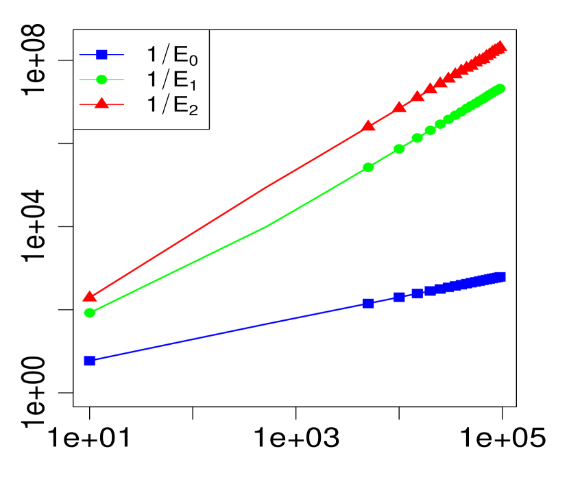
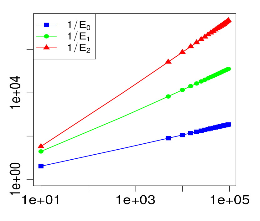
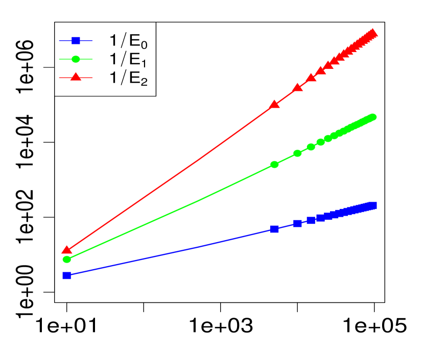
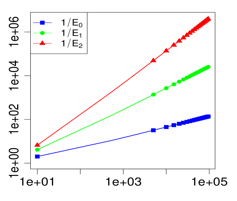
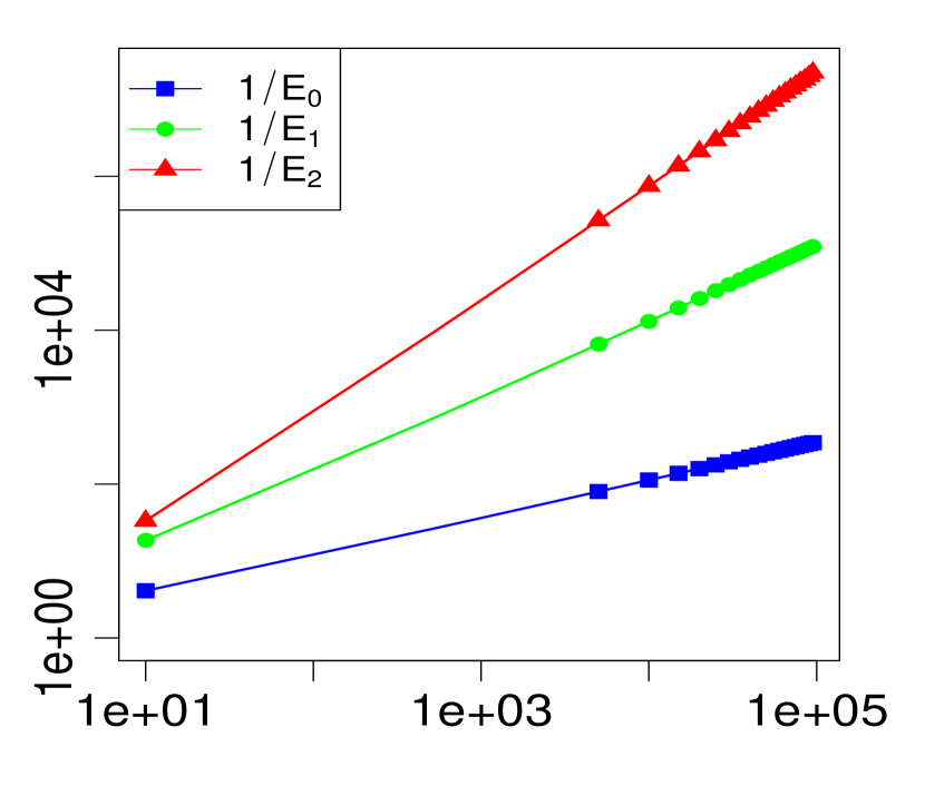
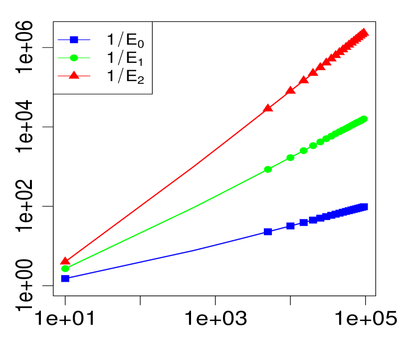
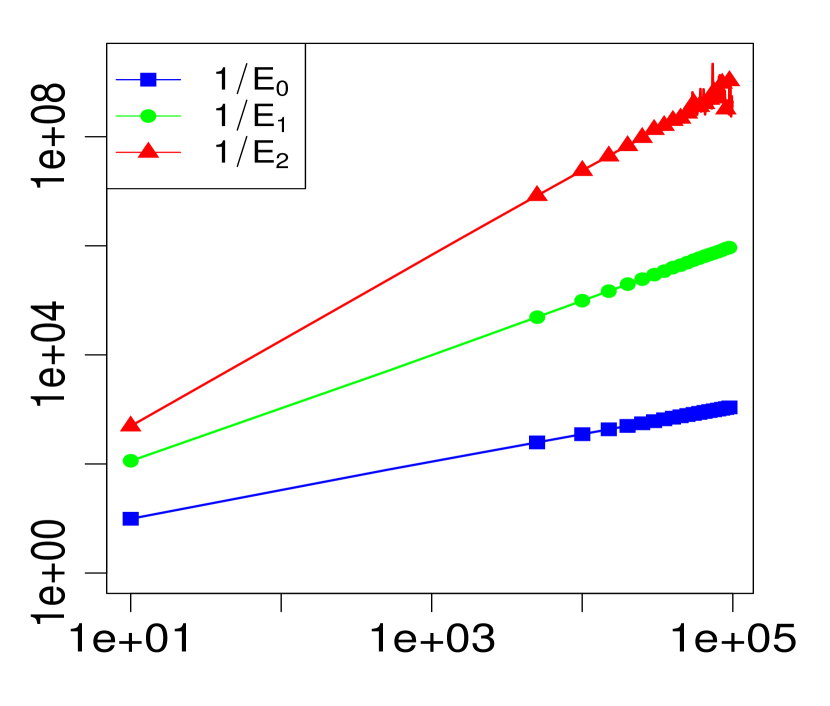
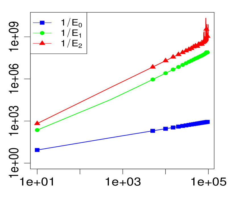
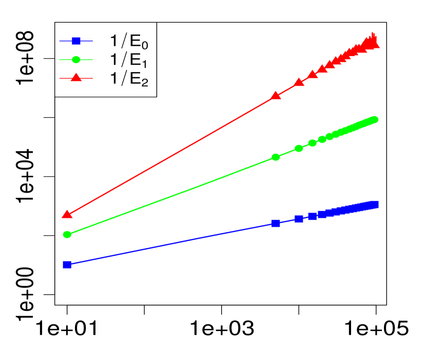
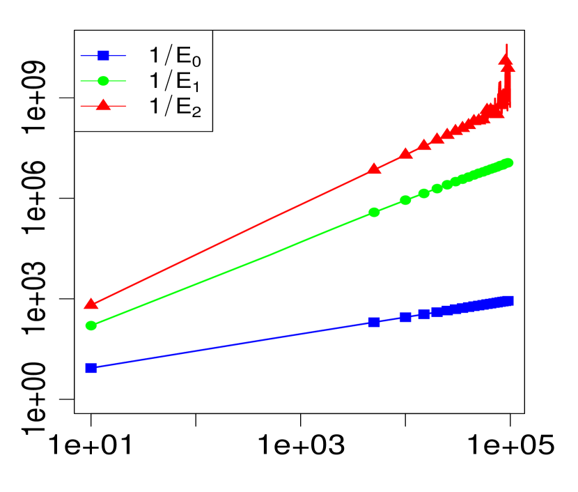
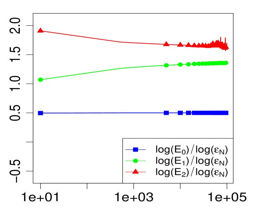
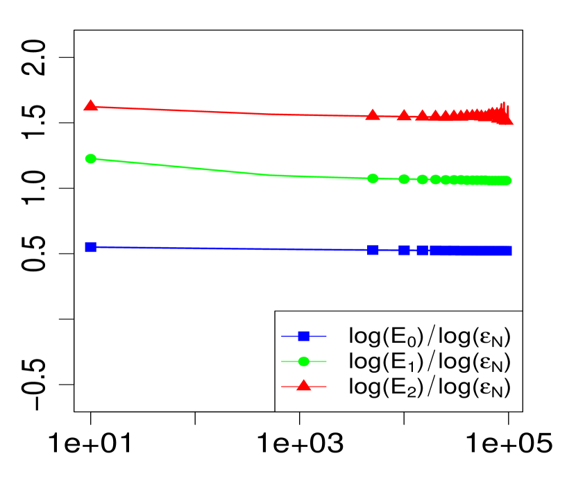
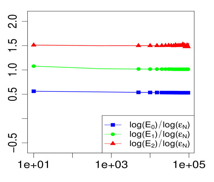
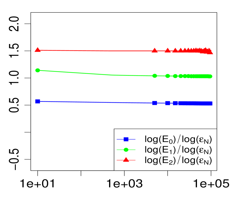
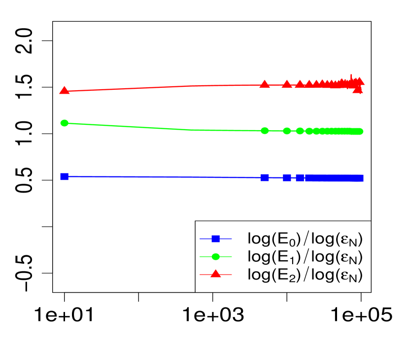
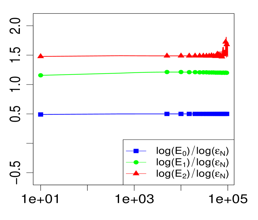
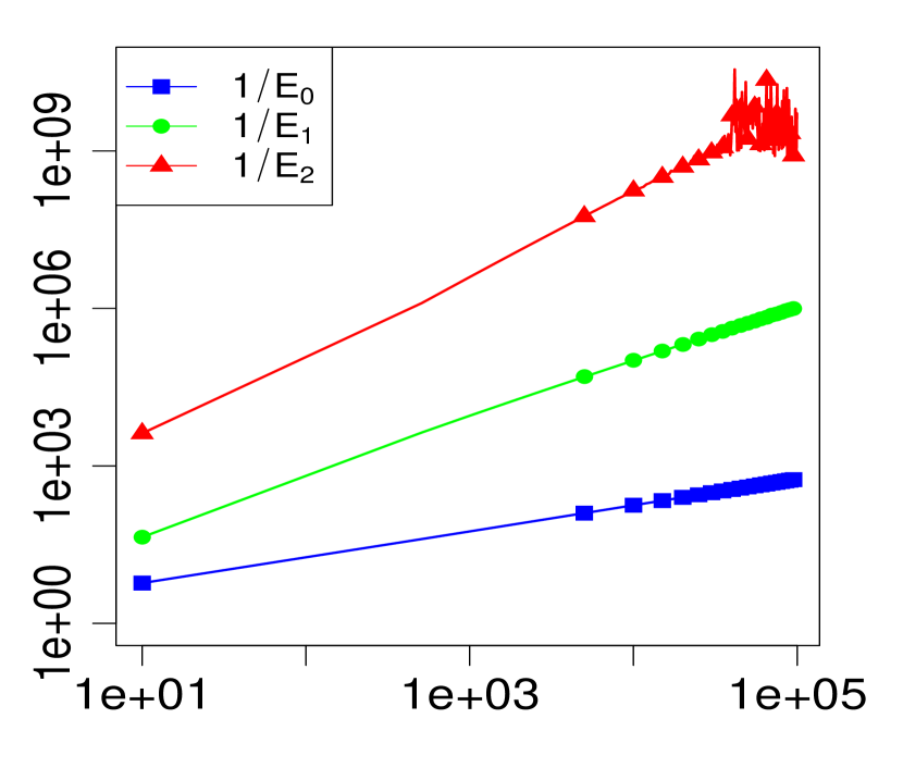
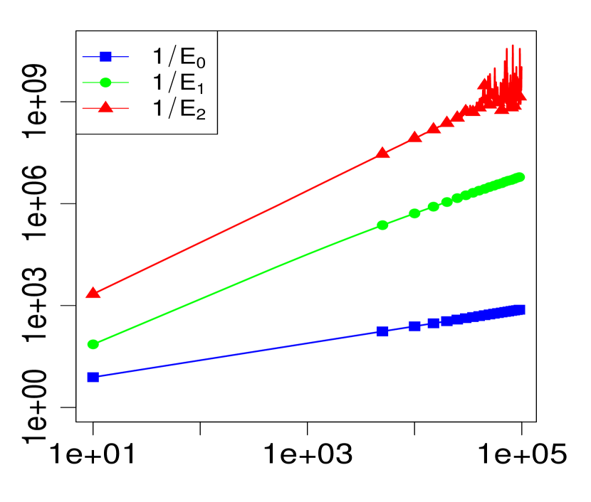
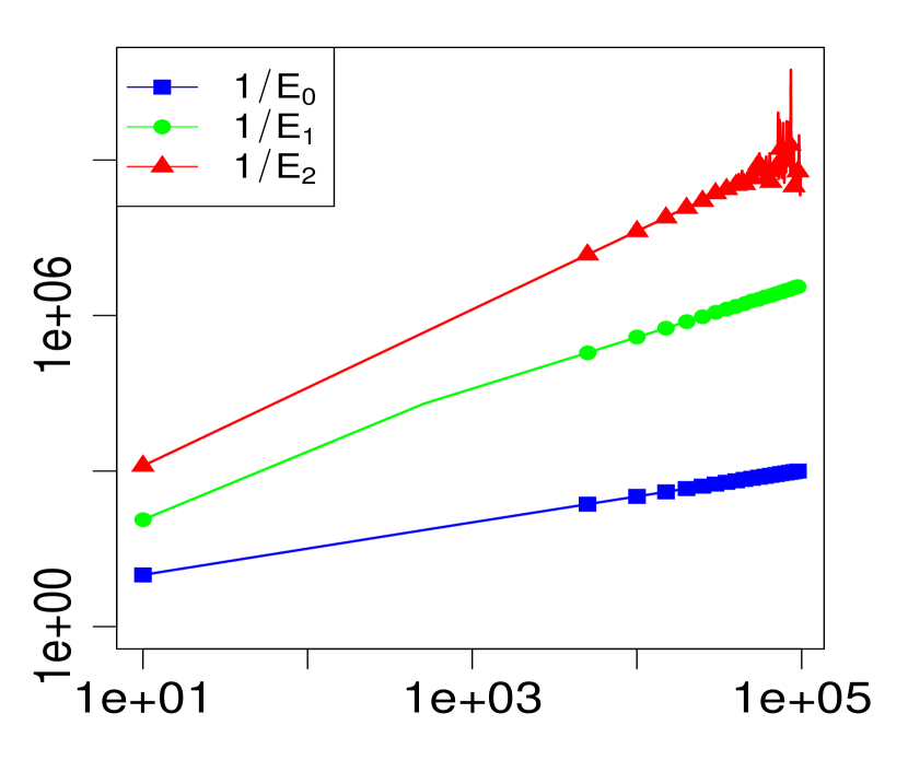
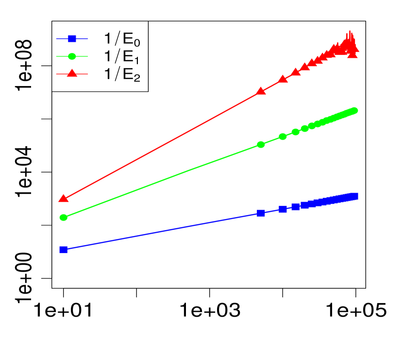
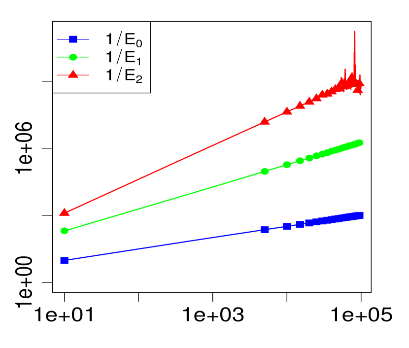
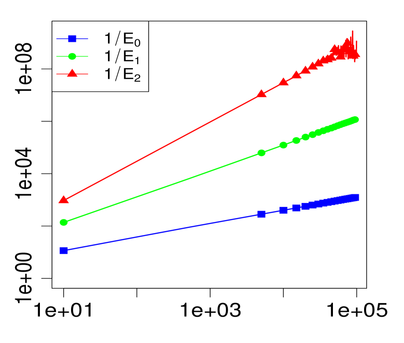
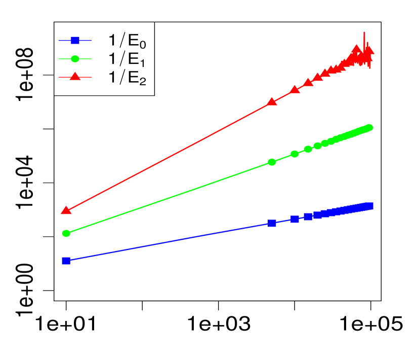
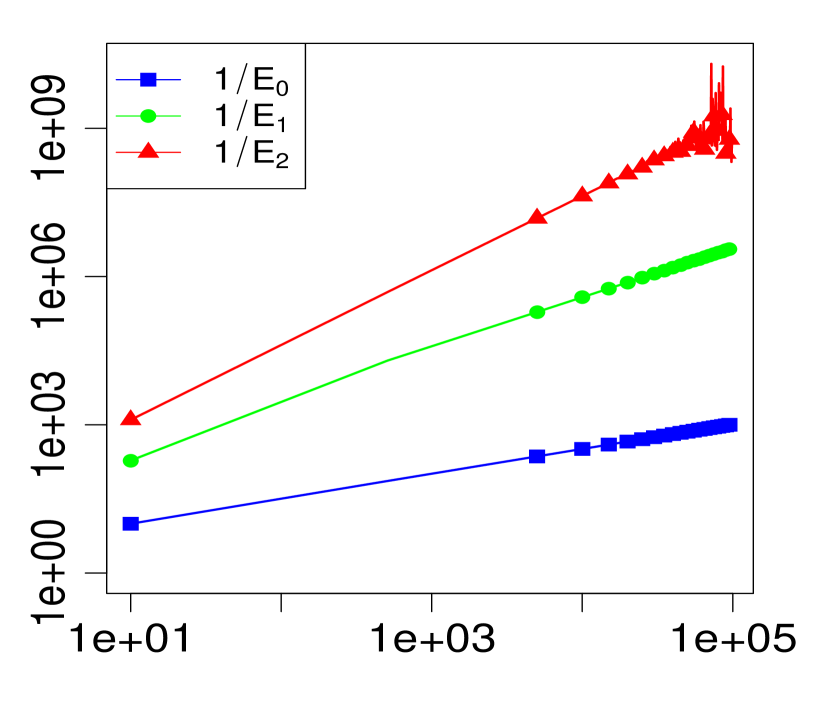
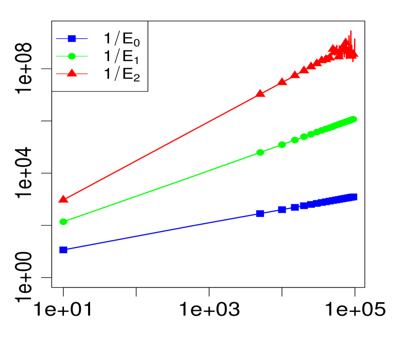
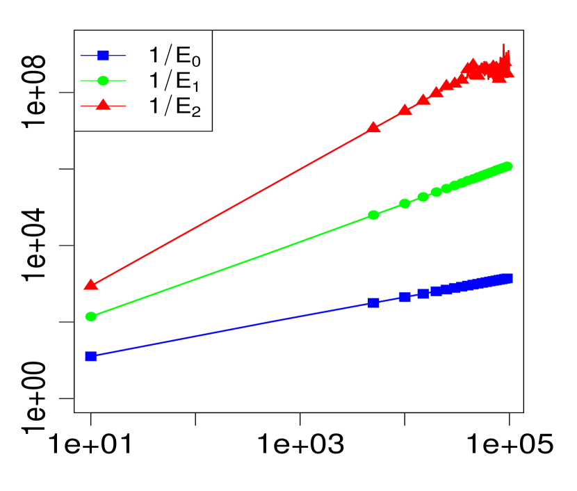
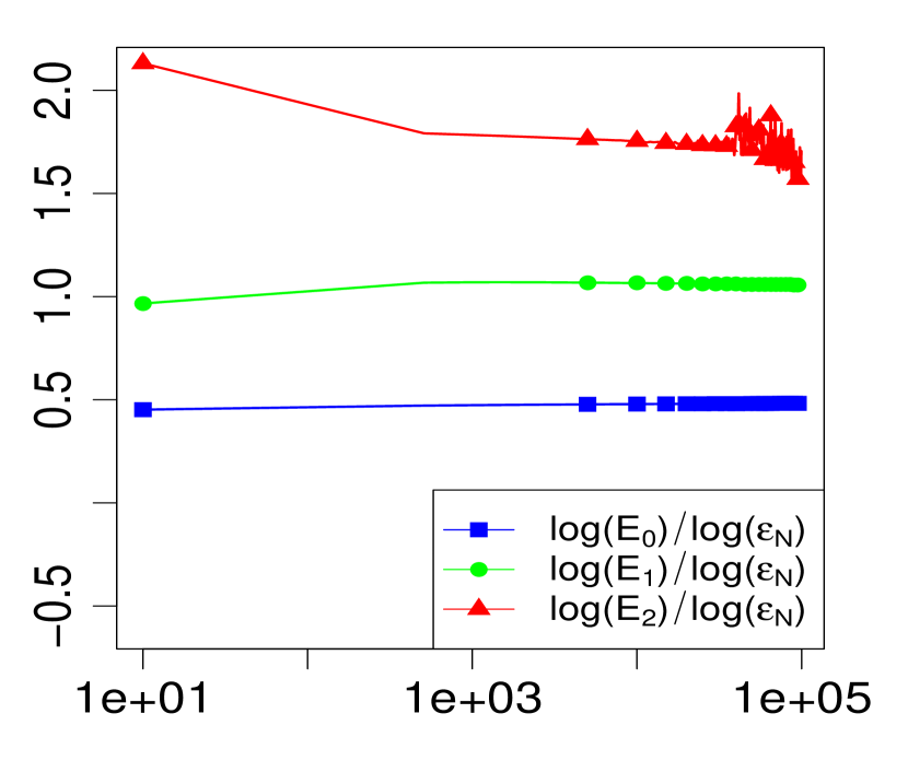
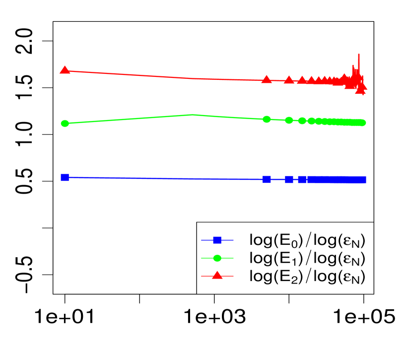
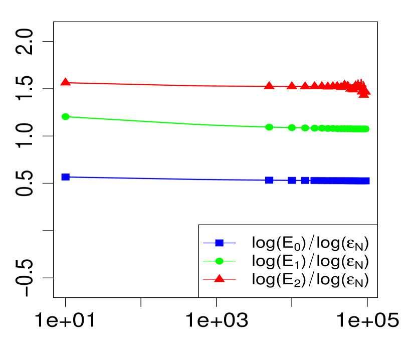
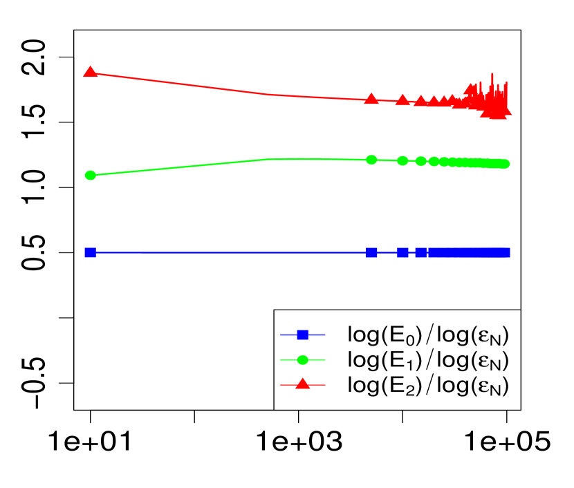
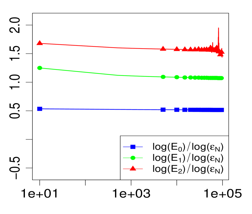
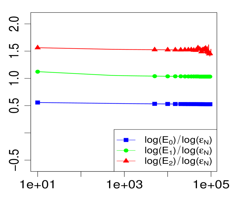
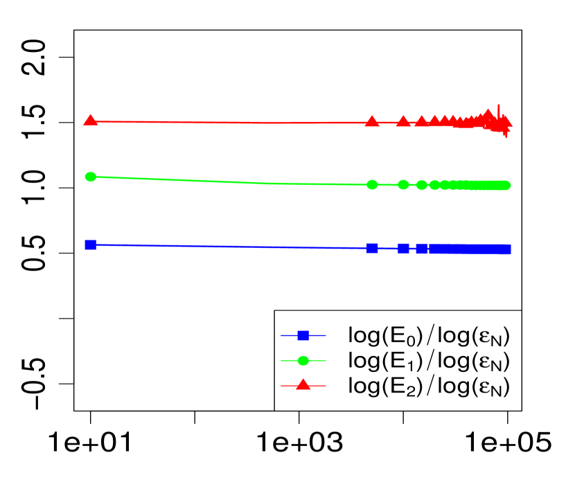
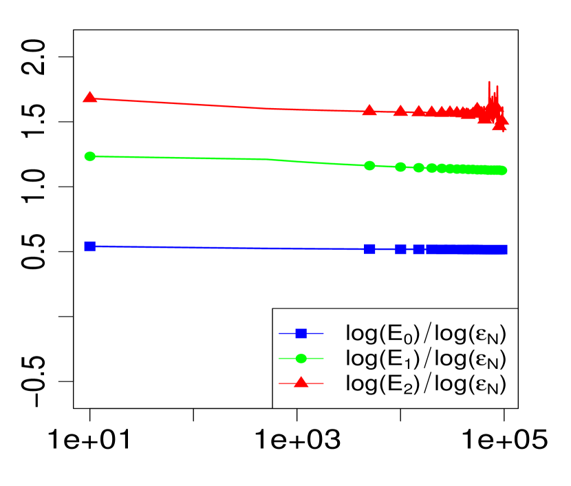
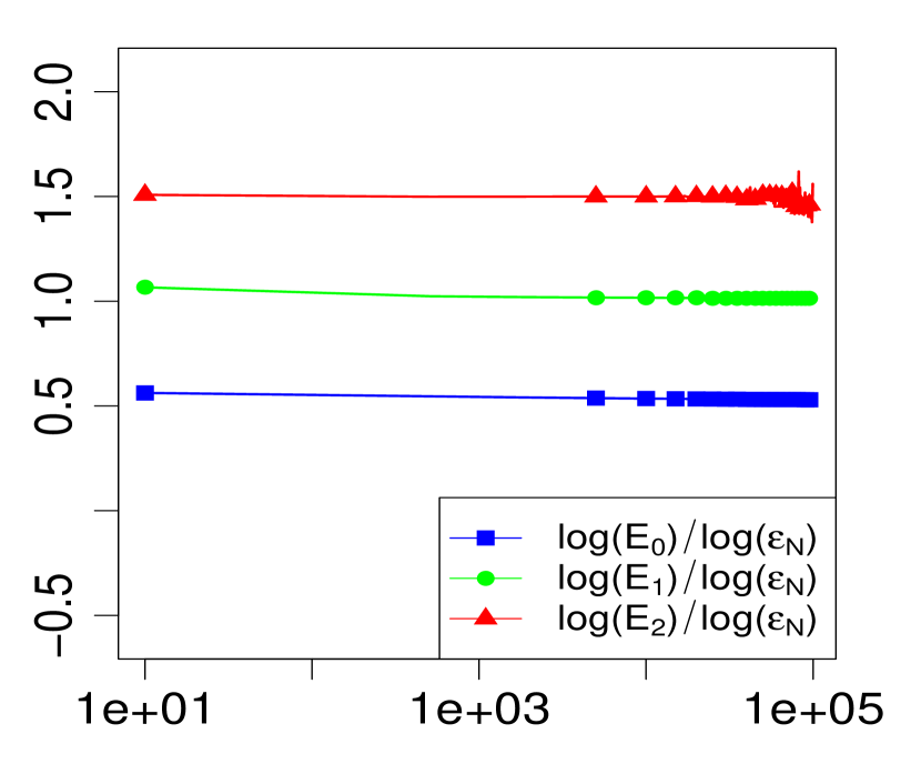
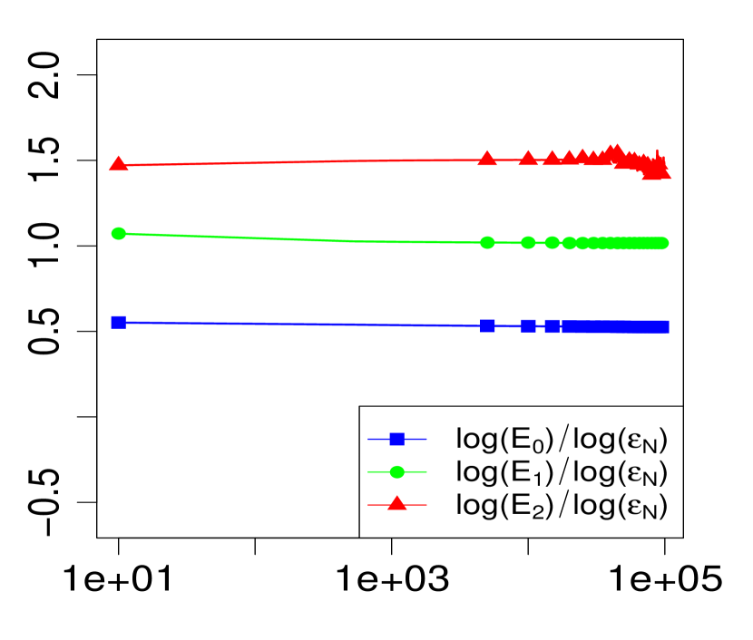
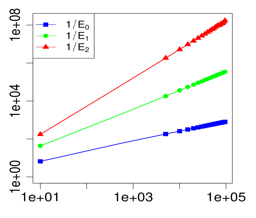
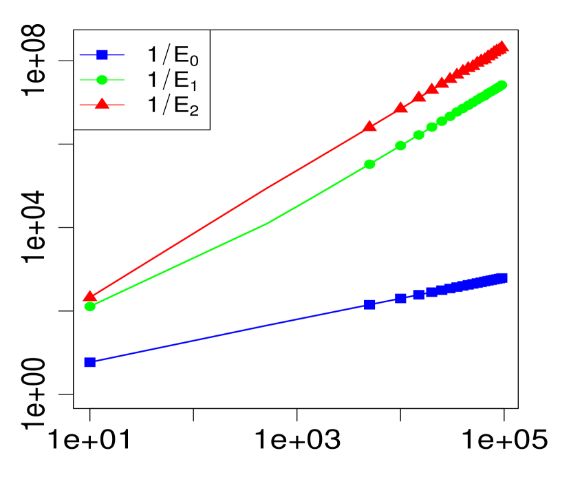
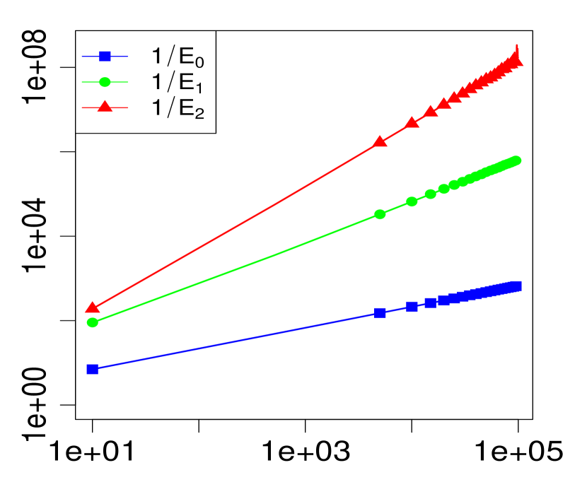
In this appendix, we provide some numerical evidence (displayed graphically) for the validity of the expansion in Theorem 2.1. We compare three levels of approximation for various choices of 𝜶𝜶\boldsymbol{\alpha} and β𝛽\beta. For any given (𝜶,β)(0,)d+1𝜶𝛽superscript0𝑑1(\boldsymbol{\alpha},\beta)\in(0,\infty)^{d+1}, define

E0subscript𝐸0\displaystyle E_{0} :=sup𝒙d:𝒙𝒓εN1/2|log(KN,𝜶,β(𝒙)(1+εN1)d/2ϕΣ𝒓(𝜹𝒙))|,assignabsentsubscriptsupremum:𝒙superscript𝑑subscriptnorm𝒙𝒓superscriptsubscript𝜀𝑁12subscript𝐾𝑁𝜶𝛽𝒙superscript1superscriptsubscript𝜀𝑁1𝑑2subscriptitalic-ϕsubscriptΣ𝒓subscript𝜹𝒙\displaystyle\vcentcolon=\sup_{\boldsymbol{x}\in\mathbb{R}^{d}:\|\boldsymbol{x}-\boldsymbol{r}\|_{\infty}\leq\varepsilon_{N}^{1/2}}\left|\log\left(\frac{K_{N,\boldsymbol{\alpha},\beta}(\boldsymbol{x})}{(1+\varepsilon_{N}^{-1})^{d/2}\phi_{\Sigma_{\boldsymbol{r}}}(\boldsymbol{\delta}_{\boldsymbol{x}})}\right)\right|, (58)
E1subscript𝐸1\displaystyle E_{1} :=sup𝒙d:𝒙𝒓εN1/2|log(KN,𝜶,β(𝒙)(1+εN1)d/2ϕΣ𝒓(𝜹𝒙))εN1/2{i=1d+1(δi,xiri)+13i=1d+1δi,xi(δi,xiri)2}|,assignabsentsubscriptsupremum:𝒙superscript𝑑subscriptnorm𝒙𝒓superscriptsubscript𝜀𝑁12subscript𝐾𝑁𝜶𝛽𝒙superscript1superscriptsubscript𝜀𝑁1𝑑2subscriptitalic-ϕsubscriptΣ𝒓subscript𝜹𝒙superscriptsubscript𝜀𝑁12superscriptsubscript𝑖1𝑑1subscript𝛿𝑖subscript𝑥𝑖subscript𝑟𝑖13superscriptsubscript𝑖1𝑑1subscript𝛿𝑖subscript𝑥𝑖superscriptsubscript𝛿𝑖subscript𝑥𝑖subscript𝑟𝑖2\displaystyle\vcentcolon=\sup_{\boldsymbol{x}\in\mathbb{R}^{d}:\|\boldsymbol{x}-\boldsymbol{r}\|_{\infty}\leq\varepsilon_{N}^{1/2}}\left|\log\left(\frac{K_{N,\boldsymbol{\alpha},\beta}(\boldsymbol{x})}{(1+\varepsilon_{N}^{-1})^{d/2}\phi_{\Sigma_{\boldsymbol{r}}}(\boldsymbol{\delta}_{\boldsymbol{x}})}\right)-\varepsilon_{N}^{1/2}\cdot\left\{-\sum_{i=1}^{d+1}\bigg{(}\frac{\delta_{i,x_{i}}}{r_{i}}\bigg{)}+\frac{1}{3}\sum_{i=1}^{d+1}\delta_{i,x_{i}}\bigg{(}\frac{\delta_{i,x_{i}}}{r_{i}}\bigg{)}^{2}\right\}\right|, (59)
E2subscript𝐸2\displaystyle E_{2} :=sup𝒙d:𝒙𝒓εN1/2|log(KN,𝜶,β(𝒙)(1+εN1)d/2ϕΣ𝒓(𝜹𝒙))εN1/2{i=1d+1(δi,xiri)+13i=1d+1δi,xi(δi,xiri)2}assignabsentconditionalsubscriptsupremum:𝒙superscript𝑑subscriptnorm𝒙𝒓superscriptsubscript𝜀𝑁12subscript𝐾𝑁𝜶𝛽𝒙superscript1superscriptsubscript𝜀𝑁1𝑑2subscriptitalic-ϕsubscriptΣ𝒓subscript𝜹𝒙superscriptsubscript𝜀𝑁12superscriptsubscript𝑖1𝑑1subscript𝛿𝑖subscript𝑥𝑖subscript𝑟𝑖13superscriptsubscript𝑖1𝑑1subscript𝛿𝑖subscript𝑥𝑖superscriptsubscript𝛿𝑖subscript𝑥𝑖subscript𝑟𝑖2\displaystyle\vcentcolon=\sup_{\boldsymbol{x}\in\mathbb{R}^{d}:\|\boldsymbol{x}-\boldsymbol{r}\|_{\infty}\leq\varepsilon_{N}^{1/2}}\left|\log\left(\frac{K_{N,\boldsymbol{\alpha},\beta}(\boldsymbol{x})}{(1+\varepsilon_{N}^{-1})^{d/2}\phi_{\Sigma_{\boldsymbol{r}}}(\boldsymbol{\delta}_{\boldsymbol{x}})}\right)-\varepsilon_{N}^{1/2}\cdot\left\{-\sum_{i=1}^{d+1}\bigg{(}\frac{\delta_{i,x_{i}}}{r_{i}}\bigg{)}+\frac{1}{3}\sum_{i=1}^{d+1}\delta_{i,x_{i}}\bigg{(}\frac{\delta_{i,x_{i}}}{r_{i}}\bigg{)}^{2}\right\}\right.
εN{12i=1d+1(1+ri)(δi,xiri)214i=1d+1δi,xi(δi,xiri)3d2+112{1i=1d+1ri1}}|.\displaystyle\quad\left.\hskip 71.13188pt-\varepsilon_{N}\cdot\left\{\frac{1}{2}\sum_{i=1}^{d+1}(1+r_{i})\bigg{(}\frac{\delta_{i,x_{i}}}{r_{i}}\bigg{)}^{2}-\frac{1}{4}\sum_{i=1}^{d+1}\delta_{i,x_{i}}\bigg{(}\frac{\delta_{i,x_{i}}}{r_{i}}\bigg{)}^{3}-\frac{d}{2}+\frac{1}{12}\Big{\{}1-\sum_{i=1}^{d+1}r_{i}^{-1}\Big{\}}\right\}\right|. (60)

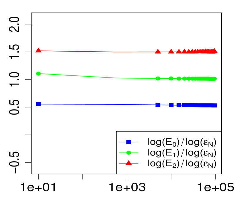
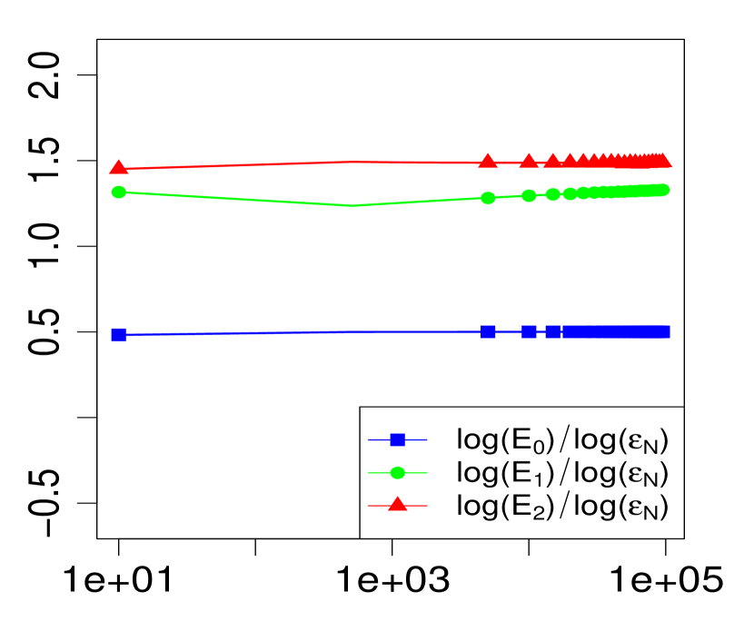
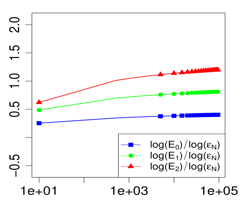
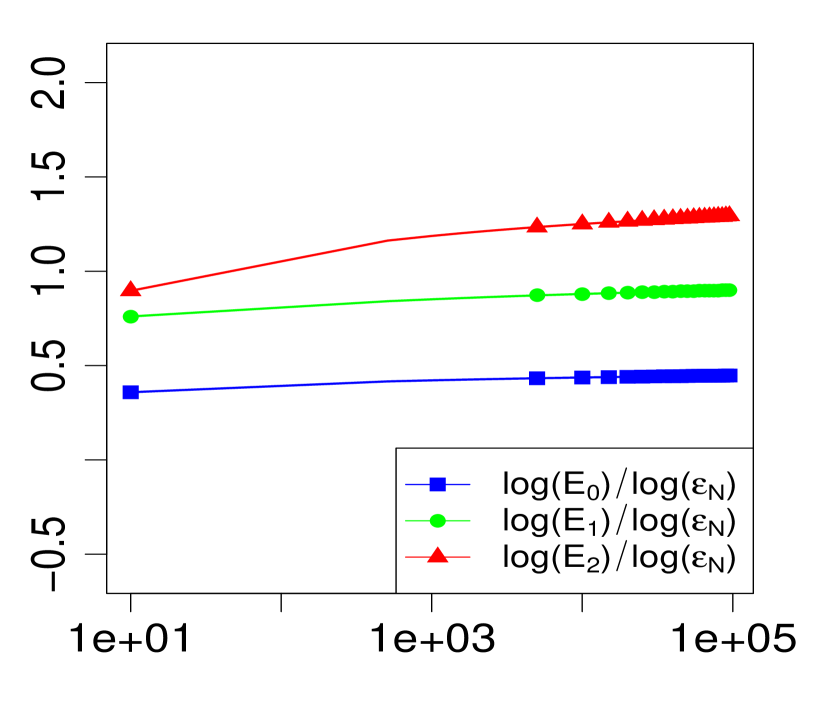
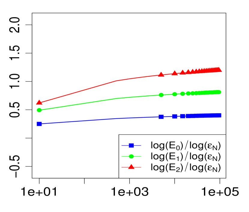
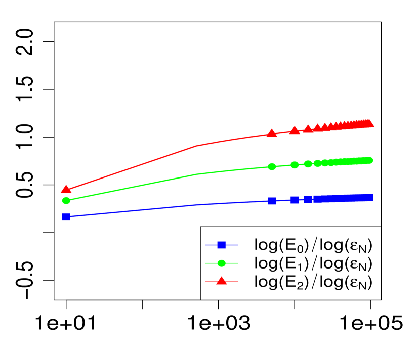
Note that 𝒙𝒓εN1/2subscriptnorm𝒙𝒓superscriptsubscript𝜀𝑁12\|\boldsymbol{x}-\boldsymbol{r}\|_{\infty}\leq\varepsilon_{N}^{1/2} implies 𝜹𝒙(1+εN)1/21subscriptnormsubscript𝜹𝒙superscript1subscript𝜀𝑁121\|\boldsymbol{\delta}_{\boldsymbol{x}}\|_{\infty}\leq(1+\varepsilon_{N})^{1/2}\approx 1, so we expect from Theorem 2.1 that the errors above (E0subscript𝐸0E_{0}, E1subscript𝐸1E_{1} and E2subscript𝐸2E_{2}) will have the asymptotic behavior

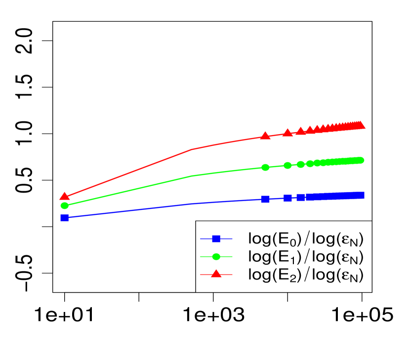
Ei=𝒪d,𝜶,β(εN(1+i)/2),for all i{0,1,2},formulae-sequencesubscript𝐸𝑖subscript𝒪𝑑𝜶𝛽superscriptsubscript𝜀𝑁1𝑖2for all 𝑖012\displaystyle E_{i}=\mathcal{O}_{d,\boldsymbol{\alpha},\beta}(\varepsilon_{N}^{(1+i)/2}),\quad\text{for all }i\in\{0,1,2\}, (61)

or equivalently,

lim infNlogEilogεN1+i2,for all i{0,1,2}.formulae-sequencesubscriptlimit-infimum𝑁subscript𝐸𝑖subscript𝜀𝑁1𝑖2for all 𝑖012\displaystyle\liminf_{N\to\infty}\frac{\log E_{i}}{\log\varepsilon_{N}}\geq\frac{1+i}{2},\quad\text{for all }i\in\{0,1,2\}. (62)

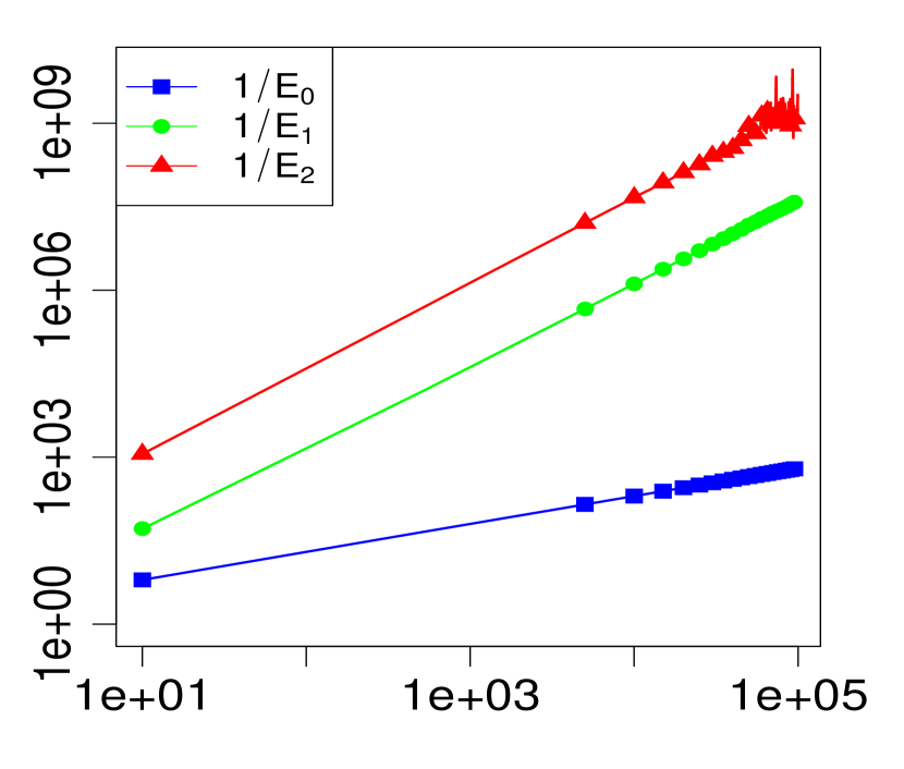
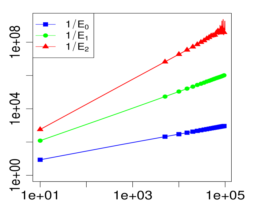
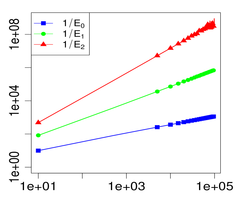
The property (62) is illustrated in Figures 24 and 6 below, for various choices of 𝜶𝜶\boldsymbol{\alpha} and β𝛽\beta. Similarly, the corresponding the log-log plots of the errors as a function of N𝑁N are displayed in Figures 13 and 5. The simulations are limited to N105𝑁superscript105N\leq 10^{5} because numerical errors start to perturb the results near that point, but the evidence remains overwhelming.
vertical spacing

Refer to caption
((a)) 𝜶=(1,1)𝜶11\boldsymbol{\alpha}=(1,1) and β=1𝛽1\beta=1
Refer to caption
((b)) 𝜶=(1,2)𝜶12\boldsymbol{\alpha}=(1,2) and β=1𝛽1\beta=1
Refer to caption
((c)) 𝜶=(1,3)𝜶13\boldsymbol{\alpha}=(1,3) and β=1𝛽1\beta=1
Refer to caption
((d)) 𝜶=(1,4)𝜶14\boldsymbol{\alpha}=(1,4) and β=1𝛽1\beta=1
Refer to caption
((e)) 𝜶=(2,1)𝜶21\boldsymbol{\alpha}=(2,1) and β=1𝛽1\beta=1
Refer to caption
((f)) 𝜶=(2,2)𝜶22\boldsymbol{\alpha}=(2,2) and β=1𝛽1\beta=1
Refer to caption
((g)) 𝜶=(2,3)𝜶23\boldsymbol{\alpha}=(2,3) and β=1𝛽1\beta=1
Refer to caption
((h)) 𝜶=(2,4)𝜶24\boldsymbol{\alpha}=(2,4) and β=1𝛽1\beta=1
Refer to caption
((i)) 𝜶=(3,1)𝜶31\boldsymbol{\alpha}=(3,1) and β=1𝛽1\beta=1
Refer to caption
((j)) 𝜶=(3,2)𝜶32\boldsymbol{\alpha}=(3,2) and β=1𝛽1\beta=1
Refer to caption
((k)) 𝜶=(3,3)𝜶33\boldsymbol{\alpha}=(3,3) and β=1𝛽1\beta=1
Refer to caption
((l)) 𝜶=(3,4)𝜶34\boldsymbol{\alpha}=(3,4) and β=1𝛽1\beta=1
Figure 1: Plots of 1/Ei1subscript𝐸𝑖1/E_{i} as a function of N𝑁N, for various choices of 𝜶𝜶\boldsymbol{\alpha}, when β=1𝛽1\beta=1. Both the horizontal and vertical axes are on a logarithmic scale. The plots clearly illustrate how the addition of correction terms from Theorem 2.1 to the base approximation (58) improves it.
Refer to caption
((a)) 𝜶=(1,1)𝜶11\boldsymbol{\alpha}=(1,1) and β=1𝛽1\beta=1
Refer to caption
((b)) 𝜶=(1,2)𝜶12\boldsymbol{\alpha}=(1,2) and β=1𝛽1\beta=1
Refer to caption
((c)) 𝜶=(1,3)𝜶13\boldsymbol{\alpha}=(1,3) and β=1𝛽1\beta=1
Refer to caption
((d)) 𝜶=(1,4)𝜶14\boldsymbol{\alpha}=(1,4) and β=1𝛽1\beta=1
Refer to caption
((e)) 𝜶=(2,1)𝜶21\boldsymbol{\alpha}=(2,1) and β=1𝛽1\beta=1
Refer to caption
((f)) 𝜶=(2,2)𝜶22\boldsymbol{\alpha}=(2,2) and β=1𝛽1\beta=1
Refer to caption
((g)) 𝜶=(2,3)𝜶23\boldsymbol{\alpha}=(2,3) and β=1𝛽1\beta=1
Refer to caption
((h)) 𝜶=(2,4)𝜶24\boldsymbol{\alpha}=(2,4) and β=1𝛽1\beta=1
Refer to caption
((i)) 𝜶=(3,1)𝜶31\boldsymbol{\alpha}=(3,1) and β=1𝛽1\beta=1
Refer to caption
((j)) 𝜶=(3,2)𝜶32\boldsymbol{\alpha}=(3,2) and β=1𝛽1\beta=1
Refer to caption
((k)) 𝜶=(3,3)𝜶33\boldsymbol{\alpha}=(3,3) and β=1𝛽1\beta=1
Refer to caption
((l)) 𝜶=(3,4)𝜶34\boldsymbol{\alpha}=(3,4) and β=1𝛽1\beta=1
Figure 2: Plots of logEi/logεNsubscript𝐸𝑖subscript𝜀𝑁\log E_{i}/\log\varepsilon_{N} as a function of N𝑁N, for various choices of 𝜶𝜶\boldsymbol{\alpha}, when β=1𝛽1\beta=1. The horizontal axis is on a logarithmic scale. The plots confirm (62) and bring strong evidence for the validity of Theorem 2.1.

vertical spacing

Refer to caption
((a)) 𝜶=(1,1)𝜶11\boldsymbol{\alpha}=(1,1) and β=2𝛽2\beta=2
Refer to caption
((b)) 𝜶=(1,2)𝜶12\boldsymbol{\alpha}=(1,2) and β=2𝛽2\beta=2
Refer to caption
((c)) 𝜶=(1,3)𝜶13\boldsymbol{\alpha}=(1,3) and β=2𝛽2\beta=2
Refer to caption
((d)) 𝜶=(1,4)𝜶14\boldsymbol{\alpha}=(1,4) and β=2𝛽2\beta=2
Refer to caption
((e)) 𝜶=(2,1)𝜶21\boldsymbol{\alpha}=(2,1) and β=2𝛽2\beta=2
Refer to caption
((f)) 𝜶=(2,2)𝜶22\boldsymbol{\alpha}=(2,2) and β=2𝛽2\beta=2
Refer to caption
((g)) 𝜶=(2,3)𝜶23\boldsymbol{\alpha}=(2,3) and β=2𝛽2\beta=2
Refer to caption
((h)) 𝜶=(2,4)𝜶24\boldsymbol{\alpha}=(2,4) and β=2𝛽2\beta=2
Refer to caption
((i)) 𝜶=(3,1)𝜶31\boldsymbol{\alpha}=(3,1) and β=2𝛽2\beta=2
Refer to caption
((j)) 𝜶=(3,2)𝜶32\boldsymbol{\alpha}=(3,2) and β=2𝛽2\beta=2
Refer to caption
((k)) 𝜶=(3,3)𝜶33\boldsymbol{\alpha}=(3,3) and β=2𝛽2\beta=2
Refer to caption
((l)) 𝜶=(3,4)𝜶34\boldsymbol{\alpha}=(3,4) and β=2𝛽2\beta=2
Figure 3: Plots of 1/Ei1subscript𝐸𝑖1/E_{i} as a function of N𝑁N, for various choices of 𝜶𝜶\boldsymbol{\alpha}, when β=2𝛽2\beta=2. Both the horizontal and vertical axes are on a logarithmic scale. The plots clearly illustrate how the addition of correction terms from Theorem 2.1 to the base approximation (58) improves it.
Refer to caption
((a)) 𝜶=(1,1)𝜶11\boldsymbol{\alpha}=(1,1) and β=2𝛽2\beta=2
Refer to caption
((b)) 𝜶=(1,2)𝜶12\boldsymbol{\alpha}=(1,2) and β=2𝛽2\beta=2
Refer to caption
((c)) 𝜶=(1,3)𝜶13\boldsymbol{\alpha}=(1,3) and β=2𝛽2\beta=2
Refer to caption
((d)) 𝜶=(1,4)𝜶14\boldsymbol{\alpha}=(1,4) and β=2𝛽2\beta=2
Refer to caption
((e)) 𝜶=(2,1)𝜶21\boldsymbol{\alpha}=(2,1) and β=2𝛽2\beta=2
Refer to caption
((f)) 𝜶=(2,2)𝜶22\boldsymbol{\alpha}=(2,2) and β=2𝛽2\beta=2
Refer to caption
((g)) 𝜶=(2,3)𝜶23\boldsymbol{\alpha}=(2,3) and β=2𝛽2\beta=2
Refer to caption
((h)) 𝜶=(2,4)𝜶24\boldsymbol{\alpha}=(2,4) and β=2𝛽2\beta=2
Refer to caption
((i)) 𝜶=(3,1)𝜶31\boldsymbol{\alpha}=(3,1) and β=2𝛽2\beta=2
Refer to caption
((j)) 𝜶=(3,2)𝜶32\boldsymbol{\alpha}=(3,2) and β=2𝛽2\beta=2
Refer to caption
((k)) 𝜶=(3,3)𝜶33\boldsymbol{\alpha}=(3,3) and β=2𝛽2\beta=2
Refer to caption
((l)) 𝜶=(3,4)𝜶34\boldsymbol{\alpha}=(3,4) and β=2𝛽2\beta=2
Figure 4: Plots of logEi/logεNsubscript𝐸𝑖subscript𝜀𝑁\log E_{i}/\log\varepsilon_{N} as a function of N𝑁N, for various choices of 𝜶𝜶\boldsymbol{\alpha}, when β=2𝛽2\beta=2. The horizontal axis is on a logarithmic scale. The plots confirm (62) and bring strong evidence for the validity of Theorem 2.1.

vertical spacing

Refer to caption
((a)) 𝜶=(1,1)𝜶11\boldsymbol{\alpha}=(1,1) and β=3𝛽3\beta=3
Refer to caption
((b)) 𝜶=(1,2)𝜶12\boldsymbol{\alpha}=(1,2) and β=3𝛽3\beta=3
Refer to caption
((c)) 𝜶=(1,3)𝜶13\boldsymbol{\alpha}=(1,3) and β=3𝛽3\beta=3
Refer to caption
((d)) 𝜶=(1,4)𝜶14\boldsymbol{\alpha}=(1,4) and β=3𝛽3\beta=3
Refer to caption
((e)) 𝜶=(2,1)𝜶21\boldsymbol{\alpha}=(2,1) and β=3𝛽3\beta=3
Refer to caption
((f)) 𝜶=(2,2)𝜶22\boldsymbol{\alpha}=(2,2) and β=3𝛽3\beta=3
Refer to caption
((g)) 𝜶=(2,3)𝜶23\boldsymbol{\alpha}=(2,3) and β=3𝛽3\beta=3
Refer to caption
((h)) 𝜶=(2,4)𝜶24\boldsymbol{\alpha}=(2,4) and β=3𝛽3\beta=3
Refer to caption
((i)) 𝜶=(3,1)𝜶31\boldsymbol{\alpha}=(3,1) and β=3𝛽3\beta=3
Refer to caption
((j)) 𝜶=(3,2)𝜶32\boldsymbol{\alpha}=(3,2) and β=3𝛽3\beta=3
Refer to caption
((k)) 𝜶=(3,3)𝜶33\boldsymbol{\alpha}=(3,3) and β=3𝛽3\beta=3
Refer to caption
((l)) 𝜶=(3,4)𝜶34\boldsymbol{\alpha}=(3,4) and β=3𝛽3\beta=3
Figure 5: Plots of 1/Ei1subscript𝐸𝑖1/E_{i} as a function of N𝑁N, for various choices of 𝜶𝜶\boldsymbol{\alpha}, when β=3𝛽3\beta=3. Both the horizontal and vertical axes are on a logarithmic scale. The plots clearly illustrate how the addition of correction terms from Theorem 2.1 to the base approximation (58) improves it.
Refer to caption
((a)) 𝜶=(1,1)𝜶11\boldsymbol{\alpha}=(1,1) and β=3𝛽3\beta=3
Refer to caption
((b)) 𝜶=(1,2)𝜶12\boldsymbol{\alpha}=(1,2) and β=3𝛽3\beta=3
Refer to caption
((c)) 𝜶=(1,3)𝜶13\boldsymbol{\alpha}=(1,3) and β=3𝛽3\beta=3
Refer to caption
((d)) 𝜶=(1,4)𝜶14\boldsymbol{\alpha}=(1,4) and β=3𝛽3\beta=3
Refer to caption
((e)) 𝜶=(2,1)𝜶21\boldsymbol{\alpha}=(2,1) and β=3𝛽3\beta=3
Refer to caption
((f)) 𝜶=(2,2)𝜶22\boldsymbol{\alpha}=(2,2) and β=3𝛽3\beta=3
Refer to caption
((g)) 𝜶=(2,3)𝜶23\boldsymbol{\alpha}=(2,3) and β=3𝛽3\beta=3
Refer to caption
((h)) 𝜶=(2,4)𝜶24\boldsymbol{\alpha}=(2,4) and β=3𝛽3\beta=3
Refer to caption
((i)) 𝜶=(3,1)𝜶31\boldsymbol{\alpha}=(3,1) and β=3𝛽3\beta=3
Refer to caption
((j)) 𝜶=(3,2)𝜶32\boldsymbol{\alpha}=(3,2) and β=3𝛽3\beta=3
Refer to caption
((k)) 𝜶=(3,3)𝜶33\boldsymbol{\alpha}=(3,3) and β=3𝛽3\beta=3
Refer to caption
((l)) 𝜶=(3,4)𝜶34\boldsymbol{\alpha}=(3,4) and β=3𝛽3\beta=3
Figure 6: Plots of logEi/logεNsubscript𝐸𝑖subscript𝜀𝑁\log E_{i}/\log\varepsilon_{N} as a function of N𝑁N, for various choices of 𝜶𝜶\boldsymbol{\alpha}, when β=3𝛽3\beta=3. The horizontal axis is on a logarithmic scale. The plots confirm (62) and bring strong evidence for the validity of Theorem 2.1.

Acknowledgments

The author acknowledges support of a postdoctoral fellowship from the NSERC (PDF) and the FRQNT (B3X supplement). We thank the referees for their valuable comments that led to improvements in the presentation of this paper.

Data Availability Statement

The R code that generated all the figures in Appendix B is available as supplemental material online at https://doi.org/10.1002/sta4.410.

References

  • Abramowitz \BBA Stegun \APACyear1964 \APACinsertmetastarMR0167642{APACrefauthors}Abramowitz, M.\BCBT \BBA Stegun, I\BPBIA.  \APACrefYear1964. \APACrefbtitleHandbook of Mathematical Functions with Formulas, Graphs, and Mathematical Tables Handbook of Mathematical Functions with Formulas, Graphs, and Mathematical Tables (\BVOL 55). \APACaddressPublisherFor sale by the Superintendent of Documents, U.S. Government Printing Office, Washington, D.C. \APACrefnoteMR0167642 \PrintBackRefs\CurrentBib
  • Aitchison \BBA Lauder \APACyear1985 \APACinsertmetastardoi:10.2307/2347365{APACrefauthors}Aitchison, J.\BCBT \BBA Lauder, I\BPBIJ.  \APACrefYearMonthDay1985. \BBOQ\APACrefatitleKernel density estimation for compositional data Kernel density estimation for compositional data.\BBCQ \APACjournalVolNumPagesJ. Roy. Statist. Soc. Ser. C342129–137. \APACrefnotedoi:10.2307/2347365 \PrintBackRefs\CurrentBib
  • Bhattacharya \BBA Ranga Rao \APACyear1976 \APACinsertmetastarMR0436272{APACrefauthors}Bhattacharya, R\BPBIN.\BCBT \BBA Ranga Rao, R.  \APACrefYear1976. \APACrefbtitleNormal Approximation and Asymptotic Expansions Normal Approximation and Asymptotic Expansions. \APACaddressPublisherJohn Wiley & Sons, New York-London-Sydney. \APACrefnoteMR0436272 \PrintBackRefs\CurrentBib
  • Bretagnolle \BBA Massart \APACyear1989 \APACinsertmetastarMR972783{APACrefauthors}Bretagnolle, J.\BCBT \BBA Massart, P.  \APACrefYearMonthDay1989. \BBOQ\APACrefatitleHungarian constructions from the nonasymptotic viewpoint Hungarian constructions from the nonasymptotic viewpoint.\BBCQ \APACjournalVolNumPagesAnn. Probab.171239–256. \APACrefnoteMR972783 \PrintBackRefs\CurrentBib
  • Brown \BOthers. \APACyear2002 \APACinsertmetastarMR1922538{APACrefauthors}Brown, L\BPBID., Cai, T\BPBIT., Low, M\BPBIG.\BCBL \BBA Zhang, C\BHBIH.  \APACrefYearMonthDay2002. \BBOQ\APACrefatitleAsymptotic equivalence theory for nonparametric regression with random design Asymptotic equivalence theory for nonparametric regression with random design.\BBCQ \APACjournalVolNumPagesAnn. Statist.303688–707. \APACrefnoteMR1922538 \PrintBackRefs\CurrentBib
  • Brown \BOthers. \APACyear2004 \APACinsertmetastarMR2102503{APACrefauthors}Brown, L\BPBID., Carter, A\BPBIV., Low, M\BPBIG.\BCBL \BBA Zhang, C\BHBIH.  \APACrefYearMonthDay2004. \BBOQ\APACrefatitleEquivalence theory for density estimation, Poisson processes and Gaussian white noise with drift Equivalence theory for density estimation, Poisson processes and Gaussian white noise with drift.\BBCQ \APACjournalVolNumPagesAnn. Statist.3252074–2097. \APACrefnoteMR2102503 \PrintBackRefs\CurrentBib
  • Brown \BBA Low \APACyear1996 \APACinsertmetastarMR1425958{APACrefauthors}Brown, L\BPBID.\BCBT \BBA Low, M\BPBIG.  \APACrefYearMonthDay1996. \BBOQ\APACrefatitleAsymptotic equivalence of nonparametric regression and white noise Asymptotic equivalence of nonparametric regression and white noise.\BBCQ \APACjournalVolNumPagesAnn. Statist.2462384–2398. \APACrefnoteMR1425958 \PrintBackRefs\CurrentBib
  • Brown \BBA Zhang \APACyear1998 \APACinsertmetastarMR1611772{APACrefauthors}Brown, L\BPBID.\BCBT \BBA Zhang, C\BHBIH.  \APACrefYearMonthDay1998. \BBOQ\APACrefatitleAsymptotic nonequivalence of nonparametric experiments when the smoothness index is 1/2121/2 Asymptotic nonequivalence of nonparametric experiments when the smoothness index is 1/2121/2.\BBCQ \APACjournalVolNumPagesAnn. Statist.261279–287. \APACrefnoteMR1611772 \PrintBackRefs\CurrentBib
  • Cai \BBA Zhou \APACyear2009 \APACinsertmetastarMR2549558{APACrefauthors}Cai, T\BPBIT.\BCBT \BBA Zhou, H\BPBIH.  \APACrefYearMonthDay2009. \BBOQ\APACrefatitleAsymptotic equivalence and adaptive estimation for robust nonparametric regression Asymptotic equivalence and adaptive estimation for robust nonparametric regression.\BBCQ \APACjournalVolNumPagesAnn. Statist.376A3204–3235. \APACrefnoteMR2549558 \PrintBackRefs\CurrentBib
  • Carter \APACyear2002 \APACinsertmetastarMR1922539{APACrefauthors}Carter, A\BPBIV.  \APACrefYearMonthDay2002. \BBOQ\APACrefatitleDeficiency distance between multinomial and multivariate normal experiments. Dedicated to the memory of Lucien Le Cam Deficiency distance between multinomial and multivariate normal experiments. dedicated to the memory of lucien le cam.\BBCQ \APACjournalVolNumPagesAnn. Statist.303708–730. \APACrefnoteMR1922539 \PrintBackRefs\CurrentBib
  • Carter \APACyear2006 \APACinsertmetastarMR2202326{APACrefauthors}Carter, A\BPBIV.  \APACrefYearMonthDay2006. \BBOQ\APACrefatitleA continuous Gaussian approximation to a nonparametric regression in two dimensions A continuous Gaussian approximation to a nonparametric regression in two dimensions.\BBCQ \APACjournalVolNumPagesBernoulli121143–156. \APACrefnoteMR2202326 \PrintBackRefs\CurrentBib
  • Carter \APACyear2007 \APACinsertmetastarMR2351100{APACrefauthors}Carter, A\BPBIV.  \APACrefYearMonthDay2007. \BBOQ\APACrefatitleAsymptotic approximation of nonparametric regression experiments with unknown variances Asymptotic approximation of nonparametric regression experiments with unknown variances.\BBCQ \APACjournalVolNumPagesAnn. Statist.3541644–1673. \APACrefnoteMR2351100 \PrintBackRefs\CurrentBib
  • Chen \BOthers. \APACyear2011 \APACinsertmetastarMR2732624{APACrefauthors}Chen, L\BPBIH\BPBIY., Goldstein, L.\BCBL \BBA Shao, Q\BHBIM.  \APACrefYear2011. \APACrefbtitleNormal Approximation by Stein’s Method Normal Approximation by Stein’s Method. \APACaddressPublisherSpringer, Heidelberg. \APACrefnoteMR2732624 \PrintBackRefs\CurrentBib
  • Dinev \BBA Mattner \APACyear2013 \APACinsertmetastarMR3201658{APACrefauthors}Dinev, T.\BCBT \BBA Mattner, L.  \APACrefYearMonthDay2013. \BBOQ\APACrefatitleThe asymptotic Berry-Esseen constant for intervals The asymptotic Berry-Esseen constant for intervals.\BBCQ \APACjournalVolNumPagesTheory Probab. Appl.572323–325. \APACrefnoteMR3201658 \PrintBackRefs\CurrentBib
  • Dudley \APACyear2005 \APACinsertmetastarDudley_2005_KMT{APACrefauthors}Dudley, R\BPBIM.  \APACrefYearMonthDay2005. \BBOQ\APACrefatitleAn exposition of Bretagnolle and Massart’s proof of the KMT theorem for the uniform empirical process An exposition of bretagnolle and massart’s proof of the KMT theorem for the uniform empirical process.\BBCQ \APACjournalVolNumPagesLectures notes for a course given in Aarhus, August 1999. \APACrefnote[URL] http://citeseerx.ist.psu.edu/viewdoc/summary?doi=10.1.1.208.2546 \PrintBackRefs\CurrentBib
  • Einmahl \APACyear1989 \APACinsertmetastarMR996984{APACrefauthors}Einmahl, U.  \APACrefYearMonthDay1989. \BBOQ\APACrefatitleExtensions of results of Komlós, Major, and Tusnády to the multivariate case Extensions of results of Komlós, Major, and Tusnády to the multivariate case.\BBCQ \APACjournalVolNumPagesJ. Multivariate Anal.28120–68. \APACrefnoteMR996984 \PrintBackRefs\CurrentBib
  • Gibbs \BBA Su \APACyear2002 \APACinsertmetastardoi:10.2307/1403865{APACrefauthors}Gibbs, A\BPBIL.\BCBT \BBA Su, F\BPBIE.  \APACrefYearMonthDay2002. \BBOQ\APACrefatitleOn choosing and bounding probability metrics On choosing and bounding probability metrics.\BBCQ \APACjournalVolNumPagesInt. Stat. Rev.703419–435. \APACrefnotedoi:10.2307/1403865 \PrintBackRefs\CurrentBib
  • Golubev \BOthers. \APACyear2010 \APACinsertmetastarMR2589320{APACrefauthors}Golubev, G\BPBIK., Nussbaum, M.\BCBL \BBA Zhou, H\BPBIH.  \APACrefYearMonthDay2010. \BBOQ\APACrefatitleAsymptotic equivalence of spectral density estimation and Gaussian white noise Asymptotic equivalence of spectral density estimation and Gaussian white noise.\BBCQ \APACjournalVolNumPagesAnn. Statist.381181–214. \APACrefnoteMR2589320 \PrintBackRefs\CurrentBib
  • Grama \BBA Nussbaum \APACyear1998 \APACinsertmetastarMR1633574{APACrefauthors}Grama, I.\BCBT \BBA Nussbaum, M.  \APACrefYearMonthDay1998. \BBOQ\APACrefatitleAsymptotic equivalence for nonparametric generalized linear models Asymptotic equivalence for nonparametric generalized linear models.\BBCQ \APACjournalVolNumPagesProbab. Theory Related Fields1112167–214. \APACrefnoteMR1633574 \PrintBackRefs\CurrentBib
  • Hipp \BBA Mattner \APACyear2007 \APACinsertmetastarMR2743033{APACrefauthors}Hipp, C.\BCBT \BBA Mattner, L.  \APACrefYearMonthDay2007. \BBOQ\APACrefatitleOn the normal approximation to symmetric binomial distributions On the normal approximation to symmetric binomial distributions.\BBCQ \APACjournalVolNumPagesTeor. Veroyatn. Primen.523610–617. \APACrefnoteMR2743033 \PrintBackRefs\CurrentBib
  • Hirukawa \APACyear2018 \APACinsertmetastarMR3821525{APACrefauthors}Hirukawa, M.  \APACrefYear2018. \APACrefbtitleAsymmetric Kernel Smoothing Asymmetric Kernel Smoothing. \APACaddressPublisherSpringer, Singapore. \APACrefnoteMR3821525 \PrintBackRefs\CurrentBib
  • Kolassa \APACyear1994 \APACinsertmetastarMR1295242{APACrefauthors}Kolassa, J\BPBIE.  \APACrefYear1994. \APACrefbtitleSeries Approximation Methods in Statistics Series Approximation Methods in Statistics (\BVOL 88). \APACaddressPublisherSpringer-Verlag, New York. \APACrefnoteMR1295242 \PrintBackRefs\CurrentBib
  • Komlós \BOthers. \APACyear1975 \APACinsertmetastarMR375412{APACrefauthors}Komlós, J., Major, P.\BCBL \BBA Tusnády, G.  \APACrefYearMonthDay1975. \BBOQ\APACrefatitleAn approximation of partial sums of independent RV’s, and the sample DF. I An approximation of partial sums of independent RV’s, and the sample DF. I.\BBCQ \APACjournalVolNumPagesZ. Wahrscheinlichkeitstheorie und Verw. Gebiete32111–131. \APACrefnoteMR375412 \PrintBackRefs\CurrentBib
  • Komlós \BOthers. \APACyear1976 \APACinsertmetastarMR402883{APACrefauthors}Komlós, J., Major, P.\BCBL \BBA Tusnády, G.  \APACrefYearMonthDay1976. \BBOQ\APACrefatitleAn approximation of partial sums of independent RV’s, and the sample DF. II An approximation of partial sums of independent RV’s, and the sample DF. II.\BBCQ \APACjournalVolNumPagesZ. Wahrscheinlichkeitstheorie und Verw. Gebiete34133–58. \APACrefnoteMR402883 \PrintBackRefs\CurrentBib
  • Major \APACyear2000 \APACinsertmetastarMajor_2000_tech_report{APACrefauthors}Major, P.  \APACrefYearMonthDay2000. \APACrefbtitleThe approximation of the normalized empirical distribution function by a Brownian bridge. The approximation of the normalized empirical distribution function by a brownian bridge. \APACrefnote
    [URL] https://users.renyi.hu/~major/probability/empir.pdf \PrintBackRefs\CurrentBib
  • Marchal \BBA Arbel \APACyear2017 \APACinsertmetastarMR3718704{APACrefauthors}Marchal, O.\BCBT \BBA Arbel, J.  \APACrefYearMonthDay2017. \BBOQ\APACrefatitleOn the sub-Gaussianity of the beta and Dirichlet distributions On the sub-Gaussianity of the beta and Dirichlet distributions.\BBCQ \APACjournalVolNumPagesElectron. Commun. Probab.22Paper No. 54, 14 pp. \APACrefnoteMR3718704 \PrintBackRefs\CurrentBib
  • Mason \BBA van Zwet \APACyear1987 \APACinsertmetastarMR893903{APACrefauthors}Mason, D\BPBIM.\BCBT \BBA van Zwet, W\BPBIR.  \APACrefYearMonthDay1987. \BBOQ\APACrefatitleA refinement of the KMT inequality for the uniform empirical process A refinement of the KMT inequality for the uniform empirical process.\BBCQ \APACjournalVolNumPagesAnn. Probab.153871–884. \APACrefnoteMR893903 \PrintBackRefs\CurrentBib
  • Mason \BBA Zhou \APACyear2012 \APACinsertmetastarMR3007210{APACrefauthors}Mason, D\BPBIM.\BCBT \BBA Zhou, H\BPBIH.  \APACrefYearMonthDay2012. \BBOQ\APACrefatitleQuantile coupling inequalities and their applications Quantile coupling inequalities and their applications.\BBCQ \APACjournalVolNumPagesProbab. Surv.9439–479. \APACrefnoteMR3007210 \PrintBackRefs\CurrentBib
  • Mattner \BBA Schulz \APACyear2018 \APACinsertmetastarMR3717995{APACrefauthors}Mattner, L.\BCBT \BBA Schulz, J.  \APACrefYearMonthDay2018. \BBOQ\APACrefatitleOn normal approximations to symmetric hypergeometric laws On normal approximations to symmetric hypergeometric laws.\BBCQ \APACjournalVolNumPagesTrans. Amer. Math. Soc.3701727–748. \APACrefnoteMR3717995 \PrintBackRefs\CurrentBib
  • Meister \BBA Reiß \APACyear2013 \APACinsertmetastarMR3010397{APACrefauthors}Meister, A.\BCBT \BBA Reiß, M.  \APACrefYearMonthDay2013. \BBOQ\APACrefatitleAsymptotic equivalence for nonparametric regression with non-regular errors Asymptotic equivalence for nonparametric regression with non-regular errors.\BBCQ \APACjournalVolNumPagesProbab. Theory Related Fields1551-2201–229. \APACrefnoteMR3010397 \PrintBackRefs\CurrentBib
  • Ng \BOthers. \APACyear2011 \APACinsertmetastarMR2830563{APACrefauthors}Ng, K\BPBIW., Tian, G\BHBIL.\BCBL \BBA Tang, M\BHBIL.  \APACrefYear2011. \APACrefbtitleDirichlet and Related Distributions Dirichlet and Related Distributions. \APACaddressPublisherJohn Wiley & Sons, Ltd., Chichester. \APACrefnoteMR2830563 \PrintBackRefs\CurrentBib
  • Ouimet \APACyear2020 \APACinsertmetastararXiv:2002.06956{APACrefauthors}Ouimet, F.  \APACrefYearMonthDay2020. \BBOQ\APACrefatitleDensity estimation using Dirichlet kernels Density estimation using Dirichlet kernels.\BBCQ \APACjournalVolNumPagesPreprint1–39. \APACrefnotearXiv:2002.06956 \PrintBackRefs\CurrentBib
  • Ouimet \APACyear2021 \APACinsertmetastarMR4249129{APACrefauthors}Ouimet, F.  \APACrefYearMonthDay2021. \BBOQ\APACrefatitleA precise local limit theorem for the multinomial distribution and some applications A precise local limit theorem for the multinomial distribution and some applications.\BBCQ \APACjournalVolNumPagesJ. Statist. Plann. Inference215218–233. \APACrefnoteMR4249129 \PrintBackRefs\CurrentBib
  • Reiß \APACyear2008 \APACinsertmetastarMR2435461{APACrefauthors}Reiß, M.  \APACrefYearMonthDay2008. \BBOQ\APACrefatitleAsymptotic equivalence for nonparametric regression with multivariate and random design Asymptotic equivalence for nonparametric regression with multivariate and random design.\BBCQ \APACjournalVolNumPagesAnn. Statist.3641957–1982. \APACrefnoteMR2435461 \PrintBackRefs\CurrentBib
  • Rohde \APACyear2004 \APACinsertmetastarMR2125610{APACrefauthors}Rohde, A.  \APACrefYearMonthDay2004. \BBOQ\APACrefatitleOn the asymptotic equivalence and rate of convergence of nonparametric regression and Gaussian white noise On the asymptotic equivalence and rate of convergence of nonparametric regression and Gaussian white noise.\BBCQ \APACjournalVolNumPagesStatist. Decisions223235–243. \APACrefnoteMR2125610 \PrintBackRefs\CurrentBib
  • Tanabe \BBA Sagae \APACyear1992 \APACinsertmetastarMR1157720{APACrefauthors}Tanabe, K.\BCBT \BBA Sagae, M.  \APACrefYearMonthDay1992. \BBOQ\APACrefatitleAn exact Cholesky decomposition and the generalized inverse of the variance-covariance matrix of the multinomial distribution, with applications An exact Cholesky decomposition and the generalized inverse of the variance-covariance matrix of the multinomial distribution, with applications.\BBCQ \APACjournalVolNumPagesJ. Roy. Statist. Soc. Ser. B541211–219. \APACrefnoteMR1157720 \PrintBackRefs\CurrentBib
  • Zaitsev \APACyear1998 \APACinsertmetastarMR1616527{APACrefauthors}Zaitsev, A\BPBIY.  \APACrefYearMonthDay1998. \BBOQ\APACrefatitleMultidimensional version of the results of Komlós, Major and Tusnády for vectors with finite exponential moments Multidimensional version of the results of Komlós, Major and Tusnády for vectors with finite exponential moments.\BBCQ \APACjournalVolNumPagesESAIM Probab. Statist.241–108. \APACrefnoteMR1616527 \PrintBackRefs\CurrentBib
  • Zhou \APACyear2004 \APACinsertmetastarZhou2004phd{APACrefauthors}Zhou, H.  \APACrefYear2004.   \APACrefbtitleMinimax Estimation with Thresholding and Asymptotic Equivalence for Gaussian Variance Regression Minimax Estimation with Thresholding and Asymptotic Equivalence for Gaussian Variance Regression \APACtypeAddressSchoolPhD thesis.   \APACaddressSchoolCornell University. \PrintBackRefs\CurrentBib