On the Convergence and Optimality of Policy Gradient for Markov Coherent Risk

Abstract

In order to model risk aversion in reinforcement learning, an emerging line of research adapts familiar algorithms to optimize coherent risk functionals, a class that includes conditional value-at-risk (CVaR). Because optimizing the coherent risk is difficult in Markov decision processes, recent work tends to focus on the Markov coherent risk (MCR), a time-consistent surrogate. While, policy gradient (PG) updates have been derived for this objective, it remains unclear (i) whether PG finds a global optimum for MCR; (ii) how to estimate the gradient in a tractable manner. In this paper, we demonstrate that, in general, MCR objectives (unlike the expected return) are not gradient dominated and that stationary points are not, in general, guaranteed to be globally optimal. Moreover, we present a tight upper bound on the suboptimality of the learned policy, characterizing its dependence on the nonlinearity of the objective and the degree of risk aversion. Addressing (ii), we propose a practical implementation of PG that uses state distribution reweighting to overcome previous limitations. Through experiments, we demonstrate that when the optimality gap is small, PG can learn risk-sensitive policies. However, we find that instances with large suboptimality gaps are abundant and easy to construct, outlining an important challenge for future research.

Keywords: policy gradient, gradient dominance, coherent risk, Markov coherent risk.

1 Introduction

As reinforcement learning (RL) has emerged as a prospective technology in consequential and safety-critical domains, a burgeoning body of research seeks to optimize objectives that incorporate notions of risk sensitivity (Garcıa and Fernández, 2015), e.g., reducing variance or mitigating the worst case returns. In particular, coherent risk functionals (Artzner et al., 1999) satisfy several natural and desirable properties, subsuming the expected return, conditional value-at-risk (CVaR), mean upper semideviation, and spectral risk functionals (Acerbi, 2002). However, when directly addressing the coherent risk in Markov decision process (MDPs), owing to time inconsistency, it can be difficult to construct dynamic programming formulations or to derive the corresponding Bellman operators. Thus many researchers instead focus on the Markov coherent risk (MCR), a time-consistent surrogate (Ruszczyński and Shapiro, 2006; Tamar et al., 2015a).

While recent papers derive policy gradient (PG) updates for MCR (Tamar et al., 2015a), PG for this objective has not been proven to enjoy the same guarantees of global convergence as it has for the expected return (Agarwal et al., 2019; Bhandari and Russo, 2019). Moreover, while folk wisdom suggests that it should converge to a stationary point of the MCR, this local convergence viewpoint leaves open the critical question of how far this point can be from the global optimum.

In this paper, we analyze the global convergence of PG algorithms for optimizing the MCR, which, to the best of our knowledge, is the first investigation into its theoretical convergence. First, we prove that the MCR is not gradient dominated and thus, in general, PG may not converge to a global optimum (Section 5). We upper bound the suboptimality of the policy using a scalar notion of first-order stationarity plus necessary problem-dependent residuals reflecting the nonlinearity and risk sensitivity of the objective. Moreover, we design MDP problem instances that illustrate how these residuals are inevitable, and thus that our upper bound is tight. Next, we show that projected gradient descent of the MCR objective converges in $O(1/\sqrt{T})$ iterations to a policy with suboptimality gap quantified by the same residuals (Section 5.3). We later show that the mentioned suboptimality gap vanishes under the expected return, which is an MCR objective, recovering the convergence results of Agarwal et al. (2019).

On the practical side, we provide methods to estimate the gradient of the MCR, a task that proves difficult because it involves an expectation over a reweighted state distribution of the underlying MDP (Theorem 4.1). The weights are determined by the solution to the maximization problem in the MCR Bellman operator (Section 4.1), unique to the coherent risk functional and dependent on the current policy. In Tamar et al. (2015a), the authors make the strong assumption that the agent can sample from the reweighted distribution of the underlying MDP, which rarely holds in online settings. To relax this assumption, in the second part of our paper, we leverage recent advances in off-policy evaluation to propose an algorithm using state distribution correction (Liu et al., 2018) to tractably estimate the gradient, which can then be plugged into any policy gradient algorithm. This permits, to our knowledge, the first evaluations of PG optimization of MCR in MDPs. In our experiments (Section 7), we integrate this method into an actor-critic algorithm to demonstrate its effectiveness in optimizing MCR in a stochastic version of the Cliffwalk environment (Sutton and Barto, 2018).

2 Related Work

Risk functionals, including exponential utility (Fei et al., 2020), the mean-variance risk functional (Di Castro et al., 2012; Prashanth and Ghavamzadeh, 2013), the conditional value-at-risk (CVaR) (Tamar et al., 2015b; Chow and Ghavamzadeh, 2014) and cumulative prospect risks (Prashanth et al., 2016) are increasingly studied in the RL literature. They have been explored empirically for a number of Atari games (Bellemare et al., 2017), and in the context of such diverse applications as autonomous driving (Mavrin et al., 2019) and healthcare (Keramati et al., 2019). Many (but not all) of these risk functionals are subsumed under the class of coherent risks (Shapiro et al., 2009), which satisfy several desirable theoretical properties (Section 3).

In the MDP setting, researchers have considered the dynamic coherent risk (Chow and Ghavamzadeh, 2014), which applies the coherent risk functional directly on the (random) return over entire trajectories and the MCR objective (Tamar et al., 2015a), which applies it in a nested manner at each timestep. Pflug and Pichler (2016) shows that the two formulations are generally not equal except for the expected return and max-risk due to a property called time consistency. Time consistent risk measures satisfy the property that if a policy is risk-optimal for $T$ timesteps onward, it is also risk-optimal for $t$ timesteps onward, where $t\leq T$. Leveraging time consistency, one can rewrite MCR objectives in dynamic programming form using a Bellman operator, as derived by Ruszczyński and Shapiro (2006) and studied in the PG setting by Tamar et al. (2015a). By contrast, for the dynamic coherent risk, the Bellman optimality operator has been derived only for CVaR (Chow et al., 2015). Even for CVaR, the dynamic coherent risk is difficult to work with, requiring that we augment the state space with the continuous CVaR level $\alpha$ ($\text{CVaR}_{\alpha}(Z)$ gives the expected value of the lower $\alpha$-quantile of the random variable $Z$), and learn the optimal value for all CVaR levels. The MCR upper bounds the dynamic coherent risk, and though not always explicitly named, has seen wide usage in RL literature (Tamar et al., 2015b; Bellemare et al., 2017).

In the primary work on PG for MCR objectives, Tamar et al. (2015a) studies the general class of coherent risk functionals, introducing a (statistically) consistent sampling-based estimate of the policy gradient. However, they do not investigate convergence of the PG algorithm to local or global optima. Further, while they present an actor-critic algorithm for optimizing the MCR, they make strong sampling assumptions.

Our work makes advances on both of these fronts. Inspired by Agarwal et al. (2019); Azizzadenesheli et al. (2018); Bhandari and Russo (2019), who demonstrate the global optimality and convergence rate of PG for the expected return, our convergence analysis characterizes the suboptimality of PG for MCR. Our proposed policy gradient algorithm is inspired by the algorithm presented in Tamar et al. (2015a), utilizing state distribution correction methods first proposed by Liu et al. (2018) for off-policy evaluation and later adapted in Liu et al. (2020) for off-policy optimization.

3 Preliminaries

Let $(\Omega,\mathcal{F},P)$ denote a probability space where $\Omega$ is a finite set of outcomes, $\mathcal{F}$ is the $\sigma$-algebra over $\Omega$, and $P\in\mathcal{B}$ is a probability measure over $\mathcal{F}$ and $\mathcal{B}=\left\{\xi:\int_{\omega\in\Omega}\xi(\omega)=1,\xi(\omega)\geq 0\right\}$ is a set of probability measures. Let $\mathcal{Z}$ be the space of real-valued random variables $Z:\Omega\rightarrow\mathbb{R}$ defined over $(\Omega,\mathcal{F},P)$. A risk functional $\rho:\mathcal{Z}\rightarrow\overline{\mathbb{R}}$ maps a random variable $Z$ to a value on the extended real line $\overline{\mathbb{R}}:=\mathbb{R}\cup\{-\infty,\infty\}$. We call $\rho$ coherent if it satisfies the following four properties (Artzner et al., 1999):

1. Monotonicity: $\rho(Z_{1})\leq\rho(Z_{2})$ whenever $Z_{1}\leq Z_{2}$ almost surely;

2. Convexity: $\rho(tZ_{1}+(1-t)Z_{2})\leq t\rho(Z_{1})+(1-t)\rho(Z_{2})$ for $t\in[0,1]$;

3. Translation equivariance: $\rho(Z+c)=\rho(Z)+c,\forall c\in\mathbb{R}$;

4. Positive homogeneity: $\rho(tZ)=t\rho(Z)$ for $t>0$.

Importantly, coherent risk functionals can be uniquely expressed using the following dual representation:

Theorem 3.1.

(Shapiro et al., 2009, Theorem 6.4) A risk functional $\rho:\mathcal{Z}\to\overline{\mathbb{R}}$ is coherent if and only if there exists a convex bounded and closed set of feasible duals $\mathcal{U}$ depending on $P$, such that

$$\rho(Z)=\sup_{\xi\in\mathcal{U}(P)}\mathbb{E}[\xi Z],$$ (1)

where the risk envelope $\mathcal{U}(P)=\{\xi\in\text{dom}(\rho^{*}):\int_{\omega\in\Omega}\xi(\omega)dP(\omega)=1,\xi\geq 0\}$ and $\text{dom}(\rho^{*})$ is the domain of the Fenchel conjugate of $\rho$.

Because the set of subdifferentials is always a convex and compact set, following Tamar et al. (2015a), we write $\mathcal{U}$ using the general form below, which includes additional assumptions on smoothness:

Assumption 3.2 (General Form of Risk Envelope).

The risk envelope $\mathcal{U}(P)$ from Theorem 3.1 can be written as

$$\mathcal{U}(P)=\{ \xi:g_{e}(\xi,P)=0\quad\forall e\in\mathcal{E},f_{i}(\xi,P)\leq 0\quad\forall i\in\mathcal{I},\xi\geq 0,\mathbb{E}_{P}[\xi]=1\},$$ (2)

where $\mathcal{E},\mathcal{I}$ denote a set of equality and inequality constraints, respectively. Each constraint $g_{e}$ is affine in $\xi$, each constraint $f_{i}$ is convex in $\xi$, and there exists a strictly feasible point $\overline{\xi}$. Further, for any given $\xi$, both $g_{e}(\xi,P)$ and $f_{i}(\xi,P)$ are twice differentiable in $P$ and there exists $M>0$ such that for all $e\in\mathcal{E}$ and $i\in\mathcal{I}$,

$$\Big{\|}\frac{dg_{e}(\xi,P)}{dP}\Big{\|}_{op}\leq M\quad\text{and}\quad\Big{\|}\frac{df_{i}(\xi,P)}{dP}\Big{\|}_{op}\leq M.$$

Assumption 3.2 is satisfied by the CVaR, mean semideviation, and spectral risk functionals, and implies that the risk envelope $\mathcal{U}$ is known in explicit form. The dual representation in Theorem 3.1 indicates that coherent risk measures can be seen as the eifjcctrdujltgunddiuvvjvffvldfukdnueiejjrtik worst-case expectation of $Z$ over probability distributions reweighted by $\xi$, which must be chosen from the set of measures in the risk envelope $\mathcal{U}$ (Chow et al., 2015).

Conditional Value-at-Risk (CVaR)

CVaR, which arises frequently in the portfolio optimization and (more recently) RL literatures, corresponds to the expected return over the worst $\alpha$ fraction of outcomes. Formally, the CVaR at a level $\alpha\in[0,1]$ of a random variable $Z$ is defined as $\rho_{\text{CVaR}_{\alpha}}=\inf_{t\in\mathbb{R}}\left\{t+\frac{1}{\alpha}\mathbb{E}[(Z-t)_{+}]\right\}$. It can equivalently be expressed in the dual formulation (Theorem 3.1) using the risk envelope $\mathcal{U}_{\text{CVaR}_{\alpha}}(P)=\left\{\xi:\xi\in\Big{[}0,\frac{1}{\alpha}\Big{]},\mathbb{E}_{P}[\xi]=1\right\}$, for which the solution $\xi^{*}$ to the maximization problem in (1) can be calculated in closed form as $\xi^{*}(\omega)=\frac{1}{\alpha}$ when $Z(\omega)>\lambda^{*}$ and as $\xi^{*}(\omega)=0$ when $Z(\omega)<\lambda^{*}$, where $\lambda^{*}$ is any $(1-\alpha)$-quantile of $Z$ (Shapiro et al., 2009, Chapter 6).

4 Problem Setting

In this paper, we focus on the infinite horizon discounted Markov Decision Process (MDP) setting. An MDP is a tuple $\mathcal{M}=(\mathcal{S},\mathcal{A},C,P,\gamma,s_{0})$, where $\mathcal{S}$ is the state space, $\mathcal{A}$ is the action space, $C:\mathcal{S}\rightarrow[0,1]$ is the cost function, $P(\cdot|s,a)$ is the transition kernel, $\gamma\in[0,1)$ is the discount factor, and $s_{0}\in\mathcal{S}$ is the starting state. A stationary Markov policy $\pi_{\theta}:\mathcal{S}\rightarrow\Delta(\mathcal{A})$ parameterized by $\theta\in\mathbb{R}^{d}$ maps each state $s\in\mathcal{S}$ to a probability measure over actions $\mathcal{A}$, where $\Delta(\cdot)$ denotes the probability simplex.

Given an MDP $\mathcal{M}$ and policy $\pi_{\theta}$, consider a filtration $\mathcal{F}=\{\mathcal{F}_{t}\}_{t\geq 0}$ such that the observations sequence $(s_{0},a_{0},c_{0},\ldots,s_{t},a_{t},c_{t})$ is $\mathcal{F}_{t}$-measurable. Let $C(s_{t})$ be the $\mathcal{F}_{t}$-measurable random cost at time $t$. In this paper, we consider the Markov coherent risk (MCR) objective defined over $\{C(s_{t})\}_{t\geq 0}$.

Definition 1 (Markov Coherent Risk Objective).

Given a sequence of random costs $\{C(s_{t})\}_{t\geq 0}$, the Markov coherent risk objective is defined as

$$\rho_{\theta}(s_{0})=\Bigg{(}C(s_{0})+\gamma\rho\bigg{(}C(s_{1})+...+\gamma\rho\Big{(}C(s_{t})+\ldots\bigg{)};\pi_{\theta}\Bigg{)}.$$

The MCR is a nested discounted sum of the risk functional $\rho$ applied at each timestep to the randomness of the cost $C(s_{t})$ given the previous state $s_{t-1}$, which arises from the stochastic policy $\pi_{\theta}$ and transitions of the MDP. We are interested in solving the following optimization problem, which seeks the parameter $\theta$ that minimizes the MCR (1),

$$\min_{\theta}\rho_{\theta}(s_{0})$$ (3)

using policy gradient methods.

4.1 Value Function and Gradient

The risk-sensitive value function for an MDP $\mathcal{M}$ under the policy $\pi_{\theta}$ is defined as $V_{\theta}(s)=\rho_{\theta}(s)$. As shown in Ruszczyński (2010) and Tamar et al. (2015a), the Bellman operator for $V_{\theta}(s)$ is

$$V_{\theta}(s)=C(s)+\gamma\max_{\xi\in\mathcal{U}(P_{\theta})}\sum_{s^{\prime}}P_{\theta}(s^{\prime}|s)\xi(s^{\prime})V_{\theta}(s^{\prime}),$$ (4)

where $\mathcal{U}$ is the risk envelope defined in Theorem 3.1 and $P_{\theta}(s^{\prime}|s):=\sum_{a\in\mathcal{A}}\pi_{\theta}(a|s)P(s^{\prime}|s,a)$. Under Assumption 3.2, the value function can be re-written as

$$V_{\theta}(s)=C(s)+\gamma\max_{\xi}\min_{\lambda^{P},\lambda^{\mathcal{E}},\lambda^{\mathcal{I}}}L_{\theta,s}(\xi,\lambda^{P},\lambda^{\mathcal{E}},\lambda^{\mathcal{I}}),$$

where $L_{\theta,s}$ is the corresponding Lagrangian

$$L_{\theta,s}(\xi,\lambda^{P},\lambda^{\mathcal{E}},\lambda^{\mathcal{I}}) =\sum_{s^{\prime}}P_{\theta}(s^{\prime}|s)\xi(s^{\prime})V_{\theta}(s^{\prime})-\lambda^{P}\Big{(}\sum_{s^{\prime}}P_{\theta}(s^{\prime}|s)\xi(s^{\prime})-1\Big{)}$$

$$\quad-\sum_{e\in\mathcal{E}}\lambda^{\mathcal{E}}(e)g_{e}(\xi,P_{\theta})-\sum_{i\in\mathcal{I}}\lambda^{\mathcal{I}}(i)f_{i}(\xi,P_{\theta}).$$ (5)

For each state $s\in\mathcal{S}$, let $(\xi_{\theta,s},\lambda_{\theta,s}^{P},\lambda_{\theta,s}^{\mathcal{E}},\lambda_{\theta,s}^{\mathcal{I}})$ denote a saddle point of (5), which is guaranteed to exist under Assumption 3.2. The gradient of the value $\nabla_{\theta}V_{\theta}(s_{0})=\nabla_{\theta}\rho_{\theta}(s_{0})$ is calculated using the saddle points $(\xi_{\theta,s},\lambda_{\theta,s}^{P},\lambda_{\theta,s}^{\mathcal{E}},\lambda_{\theta,s}^{\mathcal{I}})$, and was derived in Tamar et al. (2015a). We restate this theorem below with proof in Appendix A.

Theorem 4.1.

(Tamar et al., 2015a, Theorem 5.2) Under Assumption 3.2 and assuming the likelihood ratio $\nabla_{\theta}\log\pi_{\theta}(a|s)$ is well-defined and bounded for all $(s,a)$,

$$\nabla_{\theta}V_{\theta}(s)=\mathbb{E}_{\xi_{\theta,s}}\left[\sum_{t=0}^{\infty}\gamma^{t}\nabla_{\theta}\log\pi_{\theta}(a_{t}|s_{t})h_{\theta}(s_{t},a_{t})|s_{0}=s\right],$$

where $\mathbb{E}_{\xi_{\theta,s}}$ refers to expectation with respect to trajectories generated by a Markov chain with transition probabilities $P_{\theta}(\cdot|s)\xi_{\theta,s}(\cdot)$, and

$$h_{\theta}(s,a) =\gamma\sum_{s^{\prime}}P(s^{\prime}|s,a)\bigg{[}\xi_{\theta,s}(s^{\prime})\Big{(}V_{\theta}(s^{\prime})-\lambda_{\theta,s}^{{P}}\Big{)}$$

$$\quad-\sum_{i}\lambda_{\theta,s}^{\mathcal{I}}(i)\frac{df_{i}(\xi_{\theta,s},P_{\theta})}{dP_{\theta}}-\sum_{e}\lambda_{\theta,s}^{\mathcal{E}}(e)\frac{dg_{e}(\xi_{\theta,s},P_{\theta})}{dP_{\theta}}\bigg{]}.$$ (6)

Notation

We now introduce some notation key to our analysis of policy gradient in the following sections. First, define the infinite discounted state visitation distribution under a policy $\pi_{\theta}$ and the starting state $s_{0}$ to be $d_{\pi_{\theta}}(s):=(1-\gamma)\sum_{t=0}^{\infty}\gamma^{t}P_{\pi_{\theta}}(s_{t}=s|s_{0})$, where $P_{\pi_{\theta}}(s_{t}=s|s_{0})$ is the probability that $s_{t}=s$ after executing $\pi_{\theta}$ starting from state $s_{0}$. We adopt the shorthand for these terms as $d_{\theta}$ and $P_{\theta}$, respectively, and $d_{*}$ and $P_{*}$ for the optimal policy $\pi_{*}$. Without loss of generality, we assume that that the starting state is deterministic and thus remove $s_{0}$ from our notation to avoid clutter. We next define the MDP transitions induced by $\pi_{\theta}$ and reweighted by $\{\xi_{s}\}_{s\in\mathcal{S}}$ to be $P_{\theta}^{\xi}$. Under this reweighting, the transitions are given by $P_{\theta}^{\xi}(s^{\prime}|s):=P_{\theta}(s^{\prime}|s)\xi_{s}(s^{\prime})$. The state visitation distribution under these reweighted transitions is $d^{\xi}_{\theta}(s):=(1-\gamma)\sum_{t=0}^{\infty}\gamma^{t}P_{\theta}^{\xi}(s_{t}=s|s_{0})$.

5 Global Optimality

In this section, we investigate the global optimality and convergence of PG for the MCR objective (3) and consider policies directly parameterized by $\theta\in\mathbb{R}^{|\mathcal{S}|\times|\mathcal{A}|}$, i.e. $\pi_{\theta}(a|s)=\theta_{s,a}$. We begin with an illustrative example demonstrating that risk-sensitive MCR exhibits local minima for even simple problems, which suggests that unlike the expected return, it is not gradient dominated. We formalize this result in Lemma 5.3, which states that the value optimality gap $V_{\theta}-V_{*}$ under the MCR is upper bounded by the magnitude of the gradient plus residual terms. As a result, stationary points of the MCR objective are not guaranteed to be global optima. The residuals are a consequence of the fact that, unlike in the expected return, the MCR Bellman operator (4) is nonlinear in the policy $\pi_{\theta}$ due to the maximization over $\mathcal{U}$, which is dependent on $\pi_{\theta}$. We show that the residuals vanish under the expected return, which is a Markov coherent risk objective, demonstrating that Lemma 5.3 is a generalization of the gradient domination lemma previously developed in Agarwal et al. (2019) for expected return. Moreover, we prove that there exist problem instances for which the gradient domination inequality holds with equality, demonstrating the tightness of our result. Finally, using the gradient domination lemma, we establish the convergence rate of projected gradient descent for the MCR objective.

(a)

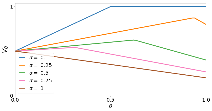
(b)

Figure 1: (a) The MDP for the bandit problem given in Section 5.1. (b) The optimization landscape for MCR using CVaR at different $\alpha$ levels in this MDP.

5.1 Motivating Example

Consider a 2-armed bandit problem where the cost of Arm 1 is a Bernoulli random variable which assigns probability $0.8$ to receiving cost $1$, and the cost of Arm 2 is always $0.5$. Suppose we work with a directly parameterized policy, where the probability of playing arm 1 is given by $\theta$ and the probability of playing arm 2 is given by $1-\theta$. This problem can equivalently be written as a five-state MDP, with transitions given in Figure 1(a).

We use the MCR objective with the $\text{CVaR}_{\alpha}$ risk functional, and in Figure 1(b), plot the optimization landscape for this problem, i.e., the MCR objective over the range of possible policies $\theta$, at different risk sensitivity levels $\alpha$. It is clear that, for a range of $\alpha<1$ levels, two stationary points exist at the boundary $\theta=0$ and $\theta=1$. Which one PG converges to depends on the initial value of $\theta$. Only when CVaR $\alpha=1$, which corresponds to the expected return, will the stationary point be unique and globally optimal. This matches previous results (Agarwal et al., 2019) demonstrating that the expected return is gradient dominated.

In addition, this counterexample exposes another source of poor convergence and suboptimality in MCR objectives. Because certain coherent risk functionals, such as $\text{CVaR}_{\alpha}$, consider a worst-case reweighted fraction of the cost distribution, they are more vulnerable to vanishing gradients than the expected return. This problem is exacerbated for higher degrees of risk sensitivity, e.g., lower $\alpha$ for CVaR. As can be seen from the $\alpha=0.1$ line in Figure 1(b), the gradient is zero for a significant fraction of random initializations of $\theta$, while expected value ($\alpha=1$) has no such problem.

5.2 Gradient Domination

We formalize the intuition of our motivating example using a property called gradient domination. Any stationary point of a gradient dominated function is also globally optimal. Even if a gradient dominated function is highly non-convex, any optimization algorithm that converges to a stationary point will also converge to a global optimum. The expected return has previously been shown to be gradient dominated. We follow the notion of gradient domination introduced by Bhandari and Russo (2019) and formally articulated in Definition 2.

Definition 2.

For $\theta\in\mathbb{R}^{d}$, a function $f$ is $(c,\mu)$- gradient dominated over $\Theta$ if there exists constants $c>0$ and $\mu\geq 0$ such that for all $\theta\in\Theta$,

$$\min_{\theta^{\prime}\in\Theta}f(\theta^{\prime})\geq f(\theta)+\min_{\theta^{\prime}\in\Theta}\Big{[}c\langle\nabla f(\theta),\theta^{\prime}-\theta\rangle+\frac{\mu}{2}\|\theta-\theta^{\prime}\|_{2}^{2}\Big{]}.$$ (7)

Definition 2 has two important implications. First, when $\langle\nabla f(\theta),\theta^{\prime}-\theta\rangle\geq 0$ for all $\theta^{\prime}$, which occurs when $\theta$ is a stationary point, we have $\min_{\theta^{\prime}\in\Theta}f(\theta^{\prime})\geq f(\theta)$, implying that $\theta$ is globally optimal. Second, for any $\theta$, the optimality gap $f(\theta)-\min_{\theta^{\prime}\in\Theta}f(\theta^{\prime})$ can be upper bounded by the minimization problem on the right hand side, which is a measure of how far $\theta$ is from stationary. We demonstrate through Lemma 5.3 that for MCR although the first statement does not hold, we can still expressively bound the optimality gap with a similar optimization problem.

We first define the two residuals presented in Lemma 5.3, which arise from two sources of nonlinearity in the Markov coherent risk value function: (i) the dependence of the saddle point solutions $\xi_{\theta,s}$ and $\lambda_{\theta,s}$ on $\pi_{\theta}$; and (ii) in the constraints $f_{i}$ and $g_{e}$ which, depending on the coherent risk measure, may be highly nonlinear in $\pi_{\theta}$. The first source of nonlinearity contributes to our analysis is the difference between the primal and dual solutions of $\pi_{\theta}$ and $\pi_{*}$, which we upper bound by $\epsilon_{L}$ in Assumption 5.1. The second source of nonlinearity contributes a residual which we upper bound by $\epsilon_{U}$ in Assumption 5.2. The residual $\epsilon_{U}$ is related to the difference between the constraint terms in the Lagrangian (5) and their first-order approximation under $\pi_{\theta}$ in the gradient update, and can be interpreted as a measure of how nonlinear the constraints are in the policy $\pi_{\theta}$.

Assumption 5.1 (Policy Residual).

Given a policy $\theta$ and any other policy $\overline{\pi}$,

$$\epsilon_{L}(\theta,\overline{\pi}):=\gamma\sum_{s}d_{\theta}^{\xi_{\theta}}(s)\Big{|}\Big{(}\lambda_{\theta,s}^{P}-\lambda_{\overline{\pi},s}^{P}\Big{)}\sum_{s^{\prime}}\Big{(}P_{\theta}-P_{\overline{\pi}}\Big{)}(s^{\prime}|s)\xi_{\theta,s}(s^{\prime})\Big{|}$$ (8)

Suppose that for all $\theta$ and $\overline{\pi}$, $\epsilon_{L}(\theta,\overline{\pi})\leq\epsilon_{L}$.

Assumption 5.2 (Constraint Residual).

Given a policy $\theta$ and any policy $\overline{\pi}$,

$$\epsilon_{U}(\theta,\overline{\pi}):= \gamma\sum_{s}d_{\theta}^{\xi_{\theta}}(s)\Big{|}\sum_{i}\lambda_{\overline{\pi},s}(i)\Delta f_{i}+\sum_{e}\lambda_{\overline{\pi},s}(e)\Delta g_{e}$$

$$+\Big{(}\pi_{\theta}-\overline{\pi}\Big{)}^{\top}\Big{(}\sum_{i}\lambda_{\theta,s}(i)\nabla_{\theta}f_{i}(\xi_{\theta},P_{\theta})+\sum_{e}\lambda_{\theta,s}(e)\nabla_{\theta}g_{e}(\xi_{\theta},P_{\theta})\Big{)}\Big{|}$$ (9)

where $\Delta f_{i}=f_{i}(\xi_{\theta},P_{\overline{\pi}})-f_{i}(\xi_{\theta},P_{\theta})$ and $\Delta g_{e}$ is defined similarly. Suppose that for all $\theta$ and $\overline{\pi}$, $\epsilon_{U}(\theta,\overline{\pi})\leq\epsilon_{U}$.

We first derive a performance difference lemma for the MCR (Appendix Lemma B.1), which upper bounds the optimality gap using an MCR advantage function. We then use it to establish the gradient domination bound in Lemma 5.3.

Lemma 5.3 (Gradient Domination).

The optimality gap $V_{\theta}(s_{0})-V_{*}(s_{0})$ is upper bounded as

$$V_{\theta}(s_{0})-V_{*}(s_{0}) \leq\Big{\|}\frac{d_{*}^{\xi_{\theta}}}{d_{\theta}^{\xi_{\theta}}}\Big{\|}_{\infty}\Big{(}\max_{\overline{\pi}\in\Delta(\mathcal{A})^{\mathcal{S}}}(\overline{\pi}-\pi_{\theta})^{\top}\nabla_{\theta}V_{\theta}(s_{0})+\epsilon_{L}(\theta,\pi_{*})+\epsilon_{U}(\theta,\pi_{*})\Big{)}.$$

Lemma 5.3 demonstrates that it is not sufficient for the gradient of the value to be small for the policy to be nearly optimal. As with previous results for expected return, the $\xi_{\theta}$-reweighted state visitation distribution $d_{\theta}^{\xi_{\theta}}$ must adequately cover the support of the reweighted state visitation distribution $d_{*}^{\xi_{\theta}}$ under the optimal policy. Whenever the fraction $\|d_{*}/d_{\theta}\|_{\infty}$, which is present in the gradient domination bound for the expected return (Agarwal et al., 2019) is finite, the term $\|d_{*}^{\xi_{\theta}}/d_{\theta}^{\xi_{\theta}}\|_{\infty}$ is also finite by definition (the converse is not necessarily true).

Further, even if $\theta$ is a stationary point, i.e., $(\overline{\pi}-\pi_{\theta})^{\top}\nabla_{\theta}V_{\theta}(s_{0})\leq 0$ for all $\overline{\pi}$, the residuals $\epsilon_{L}(\theta,\pi_{*})$ and $\epsilon_{U}(\theta,\pi_{*})$ can be nonzero and global optimality is not guaranteed. The residuals capture the distance between $\pi_{\theta}$ and an optimal policy $\pi_{*}$ in terms of the Lagrangian primal and dual variables that are used to calculate the objective function. In general, an optimal policy for a given MDP is not known a priori, but we can upper bound the optimality gap at a stationary point $\theta$ using $\max_{\overline{\pi}}\Big{[}\epsilon_{L}(\theta,\overline{\pi})+\epsilon_{U}(\theta,\overline{\pi})\Big{]}\leq\epsilon_{L}+\epsilon_{U}$ from Assumptions 5.1 and 5.2. The upper bound is problem-dependent and reflects the magnitude of risk aversion of the chosen coherent risk functional, and degree of nonlinearity in the policy arising from the risk envelope $\mathcal{U}$ in the Bellman operator (4). The residual $\epsilon_{L}$ has a larger upper bound when $\xi$ is permitted to be large, e.g., smaller fractions of the cost distribution are given a high weight. The residual $\epsilon_{U}$ is a measure of the error of a first-order approximation of the constraints $f_{i}$ and $g_{e}$, and is larger when the constraints are highly nonlinear in $\pi_{\theta}$. Roughly, the magnitude of $\epsilon_{L}$ is small when the saddle points of $\pi_{\theta}$ are close to the saddle points of the optimal policy $\pi_{*}$, and the residual $\epsilon_{U}$ is small if the constraints are additionally linear in $\pi_{\theta}$.

The expected value objective is equivalently formulated as the MCR objective for CVaR with $\alpha=1$, and its risk envelope is a singleton of $\mathcal{U}_{\text{CVaR}_{1}}(P_{\theta})=\{\xi:\xi=1\}$. As a result, $\xi_{\theta,s}=1$ for all $\theta,s$ and the expected value Bellman operator is linear in the policy. Then by definition, the residuals $\epsilon_{U}=\epsilon_{L}=0$ for expected value, and Lemma 5.3 is a generalization of the gradient domination lemma for expected return, i.e., (Lemma 4.1 in Agarwal et al. (2019)). For $\text{CVaR}_{\alpha}$, we have $\epsilon_{U}=0$ as the inequality constraints $0\leq\xi\leq\frac{1}{\alpha}$ are independent of $\pi_{\theta}$, and $\epsilon_{L}\propto\frac{1}{\alpha}$. As a result, the upper bound on the optimality gap is larger when $\alpha$ is smaller and the objective is more risk sensitive.

Moreover, Theorem 5.4 guarantees that the bound in Lemma 5.3 is in fact tight. We provide a proof sketch, with formal argument in Appendix B.

Theorem 5.4.

There exists an MDP $\mathcal{M}$ and $\pi_{\theta}$ such that

$$V_{\theta}(s_{0})-V_{*}(s_{0}) =\Big{\|}\frac{d_{*}^{\xi_{\theta}}}{d_{\theta}^{\xi_{\theta}}}\Big{\|}_{\infty}\Big{(}\max_{\overline{\pi}\in\Delta(\mathcal{A})^{\mathcal{S}}}(\overline{\pi}-\pi_{\theta})^{\top}\nabla_{\theta}V_{\theta}(s_{0})+\epsilon_{L}(\theta,\pi_{*})+\epsilon_{U}(\theta,\pi_{*})\Big{)}.$$

Proof Sketch..

We give an informal argument on the existence of the lower bound and the necessity of the residual terms. Take the CVaR at level $\alpha$ objective for example, and consider a 2-action MDP, where one action always returns a set high cost, and the other action returns a set low cost most of the time and the high cost the rest. It is easy to see that the optimal policy will always choose the latter action. However, there is a large fraction of policies in this MDP where, even if the policy chooses both actions with reasonable probabilities, the highest $\alpha$-quantile of the return distribution may include only the high cost. Thus, even though the policy may be arbitrarily suboptimal, it will have a gradient of 0. The suboptimality of the policy can be quantified exactly using the residuals terms $\epsilon_{L}(\theta,\pi_{*})$ and $\epsilon_{U}(\theta,\pi_{*})$. ∎

Remark 5.5.

Previous studies on the global optimality of PG for the expected return have taken into account two sources of suboptimality: vanishing gradients Agarwal et al. (2019) and closure under policy improvement, which Bhandari and Russo (2019) used as a condition for why some problems with constrained policy classes are gradient dominated and others are not. Our results demonstrate that neither of these is sufficient to explain suboptimality in the case of coherent risk objectives. For the latter, it is clear in our motivating example that the policy class $\theta\in[0,1]$ is closed under policy improvement.

5.3 Convergence Rates

We consider the convergence rate of projected gradient descent (PGD) on the MCR under direct policy parameterization, where updates take the following for:

$$\theta\leftarrow\text{Proj}_{\Delta(\mathcal{A})^{\mathcal{S}}}\Big{(}\theta-\eta\nabla_{\theta}V_{\theta}(s_{0})\Big{)},$$ (10)

where $\text{Proj}_{\Delta(\mathcal{A})^{\mathcal{S}}}$ is a projection on the probability simplex $\Delta(\mathcal{A})^{\mathcal{S}}$ in the Euclidean norm and $\eta$ is the learning rate. Using the gradient domination lemma, we can provide the following iteration complexity bound on PGD, with proof in Appendix B.3:

Proposition 5.6.

If $V_{\theta}$ is $\beta$-smooth in $\theta$, then the PGD algorithm in (10) on $V_{\theta}(s_{0})$ with step size $\eta=\frac{1}{\beta}$ satisfies

$$\min_{t}V_{\theta_{t}}(s_{0})-V_{*}(s_{0}) \leq D\sqrt{\frac{32|\mathcal{S}|\beta}{(1-\gamma)T}}+\epsilon_{L}+\epsilon_{U},$$

where $D=\max_{t}\|d_{*}^{\xi_{\theta_{t}}}/d_{\theta_{t}}^{\xi_{\theta_{t}}}\|_{\infty}$.

This guarantee is provided for the best policy over $T$ rounds, as is standard in the nonconvex optimization literature. This lemma demonstrates that gradient descent converges in $O(1/\sqrt{T})$ iterations, but is upper bounded by the same residuals present in the gradient domination lemma (Lemma 5.3). Even if $T\rightarrow\infty$ and the first term vanishes, it is possible for the policy to be suboptimal because the MCR objective is not gradient dominated. This phenomenon is evident in the motivating example of Section 5.1 and the optimization landscape in Figure 1(b). However, if $\epsilon_{U}$ and $\epsilon_{L}$ are additionally small, which occurs when $\theta$ is near $\pi_{*}$ or the MCR Bellman operator is (close to) linear in the policy, Proposition 5.6 demonstrates that $\theta$ is near-optimal as well. Finally, as shown previously, when the Bellman operator is linear in the policy (as is the case for expected value), the residuals vanish and we recover the convergence guarantees for PGD from Agarwal et al. (2019) for expected value.

Coherent risk functionals are not, in general, $\beta$-smooth. CVaR, for example, is considered a non-smooth optimization problem (Alexander et al., 2006), and in optimizing this objective, the authors in Tamar et al. (2015b) make the assumptions that $\frac{\partial\rho_{\theta}(Z)}{\partial\theta}$ and $\frac{\partial\lambda_{\theta}(\omega)}{\partial\theta}$ exist and are bounded. Under similar assumptions, we can guarantee $\beta$-smoothness of $V_{\theta}$ and applicability of the bound in Proposition 5.6 (proof in Appendix B.3):

Corollary 5.7.

If the gradients of the primal and dual solutions of the MCR value function (4) exist and are bounded everywhere, i.e.,

$$\Big{\|}\frac{d\xi_{\theta}}{d\theta}\Big{\|}_{\infty}\leq c\quad\text{and}\quad\Big{\|}\frac{d\lambda_{\theta}}{d\theta}\Big{\|}_{\infty}\leq c^{\prime}$$

and the second derivative of the constraints exist and are bounded, i.e., for all $e\in\mathcal{E}$ and $i\in\mathcal{I}$

$$\Big{\|}\frac{d^{2}g_{e}(\xi,P)}{dP^{2}}\Big{\|}\leq M^{\prime}\quad\text{and}\quad\Big{\|}\frac{d^{2}f_{i}(\xi,P)}{dP^{2}}\Big{\|}\leq M^{\prime}$$

then there exists $\beta$ such that the value $V_{\theta}$ is $\beta$-smooth for starting state $s_{0}$, and Proposition 5.6 holds for $V_{\theta}$.

6 Gradient Estimation

In our analysis of the global optimality of PG for MCR, we assumed access to the gradient (4.1). In practice however, the gradient is difficult to estimate because it is calculated with respect to an expectation over reweighted transitions $P_{\theta}^{\xi_{\theta}}$. Tamar et al. (2015a) propose an actor-critic method for optimizing the MCR, but require the ability to sample from an MDP with reweighted transitions $P_{\theta}^{\xi_{\theta}}$, which is often unavailable in practice. Absent such a resource, one naive method for optimizing the MCR is to draw samples from $d_{\theta}$ and multiply each sample by its importance weight $\prod_{j=1}^{t-1}\xi_{\theta,s_{j-1}}(s_{j})$, shown in Algorithm 1.

Input:

for episode $k=1...K$ do

       Generate $N$ trajectories $\tau_{k}=\{s_{0}^{(n)},a_{0}^{(n)},c_{0}^{(n)},...,s_{T}^{(n)},a_{T}^{(n)},c_{T}^{(n)}\}_{n=1}^{N}$;

       Solve the maximization problem in (5) to obtain $\widehat{\xi}_{k},\widehat{\lambda}_{k}^{P},\widehat{\lambda}_{k}^{\mathcal{E}},\widehat{\lambda}_{k}^{\mathcal{I}}$ for all $(s,s^{\prime})$;

       Compute $\widehat{h}_{k}(s,a)$ in (4.1);

       Compute $\nabla_{\theta}V_{\theta}=\sum_{n=1}^{N}\sum_{t=0}^{T}\gamma^{t}\Big{(}\prod_{j=1}^{t-1}\widehat{\xi}_{k,s_{j-1}}(s_{j})\Big{)}\widehat{h}_{k}(s_{t},a_{t})$;

       Update $\theta_{k+1}\leftarrow\theta_{k}-\eta\nabla_{\theta}V_{\theta}$;

      

end for

Algorithm 1 Importance Sampling Gradient Estimation

However, as demonstrated by Liu et al. (2018), importance sampling suffers from variance that is exponential in the time horizon. This especially concerning for smaller CVaR levels $\alpha$, as the maximum per-step importance weight is $\frac{1}{\alpha}$, which can cause the magnitude of the gradient to become intractably large in longer horizons. Instead, we propose a practical method for optimizing the MCR that leverages recent advances in off-policy evaluation and optimization. Moreover, we empirically demonstrate its improved stability and efficacy.

6.1 State Distribution Reweighting

Note that, using the stationary state distribution, we can write the gradient in (4.1) as

$$\nabla_{\theta}V_{\theta} =\sum_{s}d_{\theta}^{\xi_{\theta}}(s)\sum_{a}\pi_{\theta}(a|s)\nabla_{\theta}\log\pi_{\theta}(a|s)h_{\theta}(s,a)$$

$$=\sum_{s:d_{\theta}(s)>0}d_{\theta}(s)w_{\xi_{\theta}}(s)\sum_{a}\pi_{\theta}(a|s)\nabla_{\theta}\log\pi_{\theta}(a|s)h_{\theta}(s,a),$$ (11)

where $w_{\xi_{\theta}}(s):=d_{\theta}^{\xi_{\theta}}(s)/d_{\theta}(s)$, which is well-defined because $d_{\theta}^{\xi_{\theta}}$ is always 0 whenever $d_{\theta}$ is 0 by definition. If we can estimate the ratio $w_{\xi_{\theta}}$, then we can calculate the gradient by sampling from the original stationary state distribution $d_{\theta}$. We now state a theorem that can be used to derive the state distribution correction factor $w_{\xi_{\theta}}$, inspired by Theorem 4 of Liu et al. (2018).

Theorem 6.1.

For any $\gamma\in(0,1)$ and reweighting $\{\xi_{s}\}_{s\in\mathcal{S}}$ where $\xi_{s}:\mathcal{S}\rightarrow\mathbb{R}$, define

$$L(w,f) :=\gamma\mathbb{E}_{s,s^{\prime}\sim d_{\theta}}\Big{[}\Delta(w;s,a,s^{\prime})f(s^{\prime})\Big{]}+(1-\gamma)\mathbb{E}_{s\sim d_{0}}\Big{[}\Big{(}1-w(s)\Big{)}f(s)\Big{]},$$ (12)

where $\Delta(w;s,a,s^{\prime}):=w(s)\xi_{s}(s^{\prime})-w(s^{\prime})$. Then $w(s)$ equals $w_{\xi}(s):=d^{\xi}_{\theta}(s)/d_{\theta}(s)$ if and only if $L(w,f)=0$ for any measurable test function $f$.

This theorem suggests a method for estimating the MCR gradient using samples collected from $d_{\theta}$, by first solving the maximization in (4) to obtaining $\xi_{\theta}$, then using it to solve (12) to obtain the state distribution correction $w_{\xi_{\theta}}$. The gradient can then be calculated using a sample-based estimate of (11). In high-dimensional settings, an RKHS kernel can be used for $f$ (Liu et al., 2018).

Now that we have a method for estimating the the policy gradient of the MCR, we can use it with any PG algorithm. In Algorithm 2, we propose an actor-critic algorithm for optimizing the MCR. In episode $k$, we draw trajectories using policy $\pi_{\theta_{k}}$ and use them to calculate the solutions $(\widehat{\xi}_{k},\widehat{\lambda}_{k})$ to the min-max Lagrangian problem in (5). We then derive the state distribution corrections $\widehat{w}_{k}$ from (12) using $\widehat{\xi}_{k}$ and calculate the gradient according to Theorem 4.1. The state distribution corrections $w$ and Lagrangian variables $\xi,\lambda$ can also be learned using neural networks (see discussion in Appendix C.4).

Input: Risk envelope $\mathcal{U}$, learning rate $\eta$, MDP $\mathcal{M}$.

for episode $k=1...K$  do

       Generate $N$ trajectories $\tau_{k}=\{s_{0}^{(n)},a_{0}^{(n)},c_{0}^{(n)},...\}_{n=1}^{N}$ using $\pi_{\theta_{k}}$ in $\mathcal{M}$;

       Pad $\tau_{k}$ if necessary;

       Solve the maximization problem in Eq. (4) to obtain $\widehat{\xi}_{k},\widehat{\lambda}_{k}^{P},\widehat{\lambda}_{k}^{\mathcal{E}},\widehat{\lambda}_{k}^{\mathcal{I}}$ for all $(s,s^{\prime})$;

       Solve the optimization problem in Eq. (12) to obtain $\widehat{w}_{k}$ for all $s$;

       Compute $\widehat{h}_{k}(s,a)$ in (4.1);

       Compute $\nabla_{\theta}V_{\theta}=\sum_{a,s\sim\tau_{k}}\widehat{w}_{k}(s)\nabla_{\theta}\log\pi_{\theta_{k}}(a|s)\widehat{h}_{k}(s,a)$;

       Update $\theta_{k+1}\leftarrow\theta_{k}-\eta\nabla_{\theta}V_{\theta}$;

      

end for

Algorithm 2 State Distribution Correction Actor-Critic

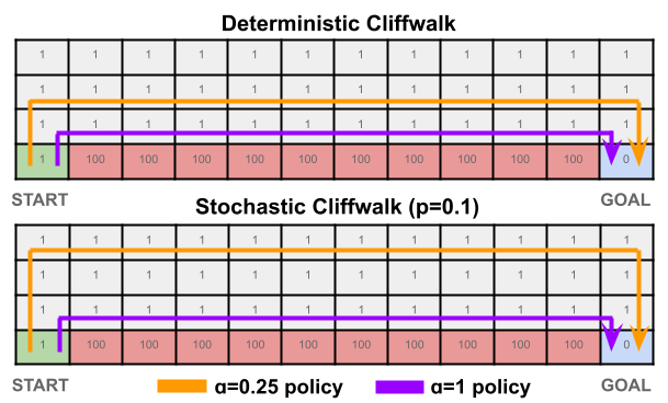
(a)

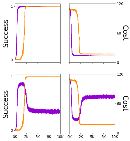
(b)

Figure 2: (a) $\text{CVaR}_{\alpha}$ policies for $\alpha=0.25$ and $\alpha=1$ learned using Algorithm 2. (b) Average cost and success (from 1000 trajectories) over training. While the learned policy for $\alpha=1$ always takes the shortest path, it fails to consistently reach the goal when the environment is stochastic.

6.2 Convergence Result

We provide a convergence result for Algorithm 2 to a stationary point of the MCR objective. First, we state the following assumption for our convergence guarantee:

Assumption 6.2.

For all state-action pairs $(s,a)$ and $\theta\in\Theta$, suppose that

1. $\Big{\|}\frac{\partial\pi_{\theta}(a|s)}{\partial\theta}\Big{\|}\leq G$

2. $V_{\theta}(s),h_{\theta}(s,a)\leq C_{max}$

3. $\sigma^{2}_{w}:=\mathbb{E}_{d_{\theta}}[w_{\xi_{\theta}}(s)^{2}]<\infty$

4. the MCR is $L$-Lipschitz and $\beta$-smooth (see Corollary 5.7)

We have previously discussed the validity of Assumption 4 in Corollary 5.7, and Assumption 3 was previously made in Liu et al. (2020). Assumption 1 can be achieved by an appropriate policy parameterization, such as through a linear or differentiable neural network function approximation with softmax output. Assumption 2 follows from the boundedness of $V_{\theta}$, an assumption common in the literature, and boundedness of the Lagrangian solutions $(\xi_{\theta},\lambda)$ present in the calculation of $h_{\theta}$ (4.1). Boundedness of $\xi$ is guaranteed by the constraints in $\mathcal{U}$. The MCR objective with $\text{CVaR}_{\alpha}$ satisfies Assumption 2, for example, because $|\xi_{\theta}|\leq\frac{1}{\alpha}$ by definition, $\lambda^{P}_{\theta}$ is bounded whenever the value is bounded because it is any $(1-\alpha)$ quantile of the distribution of returns, and the remainder of the terms in $h_{\theta}$ are 0. Following this, for Algorithm 2, we can make the following convergence guarantee to a stationary point, with proof in Appendix C.2.

Theorem 6.3.

Suppose Algorithm 2 at episode $k$ and parameters $\theta_{k}$ is provided with critic estimates $\widehat{V}_{k}$, Lagrangian variable estimates $\widehat{\xi}_{k}$ and $\widehat{\lambda}_{k}$, and distribution ratio estimates $\widehat{w}_{k}$ satisfying $\mathbb{E}_{s\sim d}(w_{\theta_{k}}(s)-\widehat{w}_{k}(s))^{2}\leq\epsilon_{w,k}^{2}$ and $\mathbb{E}_{s\sim d}(h_{\theta_{k}}(s,a)-\widehat{h}_{\theta_{k}}(s,a))^{2}\leq\epsilon_{h,k}^{2}$ for all episodes $k$. Then if Assumption 6.2 is satisfied,

$$\frac{1}{K}\sum_{k=1}^{K}\mathbb{E}\Big{[}\Big{\|}\nabla_{\theta}V_{\theta_{k}}\Big{\|}^{2}\Big{]} \leq\frac{2\beta C_{max}}{\sqrt{K}}+\frac{1}{K}\sum_{k=1}^{K}\bigg{(}\frac{6}{\sqrt{K}}\Big{(}(\epsilon_{w,k}^{2}C_{max}^{2}+\epsilon_{h,k}^{2}(\sigma_{w}^{2}+\epsilon_{w,k}^{2}))G^{2}\Big{)}$$

$$\quad\quad+2L\Big{(}(\epsilon_{w,k}C_{max}+\epsilon_{h,k}\sqrt{\sigma_{w}+\epsilon_{w,k}})G\Big{)}\bigg{)}$$

Theorem 6.3 demonstrates that when Assumptions 6.2 hold, the average gradient magnitude over the $K$ episodes is upper bounded by three terms. The first two terms vanish as $K\rightarrow\infty$, but the third does not. However, since the third term is in terms of $h$ and $w$ estimation errors, given estimators $\widehat{h}$ and $\widehat{w}$ with small average error $\epsilon_{h,k},\epsilon_{w,k}$ across the episodes, the third term vanishes as $K\rightarrow\infty$ as well. Under such conditions, Theorem 6.3 shows that Algorithm 2 will converge to an approximate stationary point. Estimators for $\widehat{h}$ and $\widehat{w}$ with small average error can be achieved with a reasonable online critic and $w,\xi,\lambda$ learning algorithms. For $\text{CVaR}_{\alpha}$, $C_{max}\propto\frac{1}{\alpha}$ due to the presence of $\xi$ in the calculation of $h_{\theta}$ (4.1), implying that with higher risk sensitivity, convergence to stationary points occurs more slowly.

7 Experiments

In this section, we examine the empirical efficacy of Algorithm 2 with two primary questions in mind:

• Does the state distribution correction reduce the variance of PG on MCR in MDPs?

• Does increasing the risk envelope set $\mathcal{U}$ lead to more risk-sensitive behavior?

Baseline and Implementation.

To answer these questions, we optimize the MCR with the $\text{CVaR}_{\alpha}$ objective at different levels $\alpha$, where smaller $\alpha$ corresponds to higher risk aversion. To optimize this objective, we run Algorithm 2 and compare its performance against importance sampling baselines (Algorithm 1). For both, we use a softmax tabular policy and tabular critic. Full implementation details and a function approximation version of this algorithm are provided in Appendix C.3.

Simulation Domain.

We compare the algorithms on the classic $4\times 12$ tabular Cliffwalk environment, where the agent needs to travel from a start to a goal state while incurring as little cost as possible. Each action incurs 1 cost, but the shortest path lies next to a cliff and entering the cliff corresponds to a cost of 100. Because the classic Cliffwalk environment is deterministic, we also compare our algorithms on a stochastic version, where the row of cells above the cliff is “slippery", and induce a transition from these cells into the cliff with probability $p$. Although our algorithm is intended for an infinite-horizon MDP, the horizon is fixed to a maximum of 500 timesteps for computational feasibility.

Results.

Figure 2(a) displays the learned policies for different CVaR levels $\alpha$ in the deterministic and stochastic environments. Interestingly, the $\alpha=0.25$ policy finds a conservative policy and takes a longer path in both deterministic and stochastic Cliffwalk, even though the optimal policy in the deterministic environment is to take the shortest path for all $\alpha$ levels. In the stochastic cliffwalk, the $\alpha=1$ policy learns to take the greedy path but risks falling into the cliff, resulting in failure to consistently succeed at the task. We display the learned state distribution correction and its discussion in Appendix C.3. In both environments, the gradient of the naive importance sampling method diverged, and learning a policy was not possible in either case. In our experiments, a policy in only a truncated Cliffwalk of size $2\times 4$ was learnable via importance sampling.

8 Discussion

In this paper, we answered several open questions concerning PG for coherent risk functionals. First, we demonstrated that MCR objectives are not in general gradient dominated, giving tight upper bounds on the suboptimality of the learned policy. Second, we proposed an algorithm based on stationary state distribution reweighting to relax stringent assumptions of previous work and tractably estimate the MCR gradient. We demonstrated that our algorithm is guaranteed to converge to stationary points, and demonstrated the stability and efficacy of our algorithm on the CliffWalk environment, in which importance sampling cannot learn policies due to exploding gradient magnitudes.

While coherent risk objectives are often used in practice, our results highlight the challenges of obtaining global optimality guarantees for the final policy. One important direction of future work lies in improving these convergence results through better characterization of the residual terms over the learning process, and expanding it to other PG algorithms and settings. Further, the lower bound in Theorem 5.4 indicates that poorly conditioned starting states or initial policies also cause convergence to suboptimal policies. In the future, we will investigate how different exploration strategies, such using a combination of expected value and coherent risk, may help to mitigate this issue both in theory and practice.

Appendix

Appendix A Proofs for Section 4.1

Proof of Theorem 4.1.

The proof of this theorem is given in Appendix D of Tamar et al. [2015a], and we repeat it here for completeness. The value $V_{\theta}$ is defined as:

$$V_{\theta}(s) =C(s)+\gamma\max_{\xi\in\mathcal{U}(P_{\theta})}\sum_{s^{\prime}}P_{\theta}(s^{\prime}|s)\xi(s^{\prime})V_{\theta}(s^{\prime})$$

$$=C(s)+\gamma\max_{\xi}\min_{\lambda}L_{\theta,s}(\xi,\lambda^{P},\lambda^{\mathcal{I}},\lambda^{\mathcal{E}})$$

Using the envelope theorem [Milgrom and Segal, 2002],

$$\nabla_{\theta}V_{\theta}(s) =\gamma\nabla_{\theta}\max_{\xi}\min_{\lambda}L_{\theta,s}(\xi,\lambda^{P},\lambda^{\mathcal{I}},\lambda^{\mathcal{E}})$$

$$=\gamma\nabla_{\theta}L_{\theta,s}(\xi,\lambda^{P},\lambda^{\mathcal{I}},\lambda^{\mathcal{E}})|_{(\xi_{\theta},\lambda_{\theta}^{P},\lambda_{\theta}^{\mathcal{E}},\lambda_{\theta}^{\mathcal{I}})}$$

The derivative of the Lagrangian evaluated at the saddle point $(\xi_{\theta},\lambda_{\theta}^{P},\lambda_{\theta}^{\mathcal{E}},\lambda_{\theta}^{\mathcal{I}})$ is:

$$\nabla_{\theta}L_{\theta,s}(\xi_{\theta,s},\lambda_{\theta,s}^{P},\lambda_{\theta,s}^{\mathcal{E}},\lambda_{\theta,s}^{\mathcal{I}})$$

$$\quad=\sum_{s^{\prime}}\xi_{\theta,s}(s^{\prime})\sum_{a}\nabla_{\theta}\pi_{\theta}(a|s)P(s^{\prime}|s,a)V_{\theta}(s^{\prime})+\sum_{s^{\prime}}P_{\theta}(s^{\prime}|s)\xi_{\theta,s}(s^{\prime})\nabla_{\theta}V_{\theta}(s^{\prime})$$

$$\quad-\lambda_{\theta,s}^{P}\sum_{s^{\prime}}\xi_{\theta,s}(s^{\prime})\sum_{a}\nabla_{\theta}\pi_{\theta}(a|s)P(s^{\prime}|s,a)$$

$$\quad-\sum_{i\in\mathcal{I}}\lambda_{\theta,s}^{\mathcal{I}}(i)\frac{df_{i}(\xi_{\theta,s},P_{\theta})}{dp(s^{\prime})}\sum_{a}\nabla_{\theta}\pi_{\theta}(a|s)P(s^{\prime}|s,a)-\sum_{e\in\mathcal{E}}\lambda_{\theta,s}^{\mathcal{E}}(e)\frac{dg_{e}(\xi_{\theta,s},P_{\theta})}{dp(s^{\prime})}\sum_{a}\nabla_{\theta}\pi_{\theta}(a|s)P(s^{\prime}|s,a)$$

Then we have

$$\nabla_{\theta}V_{\theta}(s) =\gamma\sum_{s^{\prime}}P_{\theta}(s^{\prime}|s)\xi_{\theta,s}(s^{\prime})\nabla_{\theta}V_{\theta}(s^{\prime})+\sum_{a}\nabla_{\theta}\pi_{\theta}(a|s)\bigg{[}\gamma\sum_{s^{\prime}}P(s^{\prime}|s,a)\Big{[}\xi_{\theta,s}\Big{(}V_{\theta}(s^{\prime})-\lambda_{\theta,s}^{P}\Big{)}$$

$$-\sum_{i\in\mathcal{I}}\lambda_{\theta,s}^{\mathcal{I}}(i)\frac{df_{i}(\xi_{\theta,s},P_{\theta})}{dp(s^{\prime})}-\sum_{e\in\mathcal{E}}\lambda_{\theta,s}^{\mathcal{E}}(e)\frac{dg_{e}(\xi_{\theta,s},P_{\theta})}{dp(s^{\prime})}\Big{]}\bigg{]}$$

$$=\sum_{a}\nabla_{\theta}\pi_{\theta}(a|s)h_{\theta}(s,a)+\gamma\sum_{s^{\prime}}P_{\theta}(s^{\prime}|s)\xi_{\theta,s}(s^{\prime})\nabla_{\theta}V_{\theta}(s^{\prime})$$

with $h_{\theta}(s,a)$ as defined in (4.1). Unfolding the recursion, this gives us

$$\nabla_{\theta}V_{\theta}(s) =\sum_{a}\nabla_{\theta}\pi_{\theta}(a_{0}|s_{0})h_{\theta}(s_{0},a_{0})+\gamma\sum_{s_{1}}P_{\theta}(s_{1}|s_{0})\xi_{\theta,s_{0}}(s_{1})\Big{(}\nabla_{\theta}\pi_{\theta}(a_{1}|s_{1})h_{\theta}(s_{1},a_{1})$$

$$\qquad+\gamma\sum_{s_{2}}P_{\theta}(s_{2}|s_{1})\xi_{\theta,s_{1}}(s_{2})\nabla_{\theta}V_{\theta}(s_{2})\Big{)}$$

and unfolding the recursion further gives the result.

∎

Appendix B Proofs for Section 5

B.1 Proof of Lemma 5.3

We first establish the performance difference lemma (Lemma B.1) for MCR, which upper bounds the optimality gap using an advantage function. This lemma holds for all policies, not only the directly parameterized policies we consider in Section 5.

Lemma B.1 (Performance Difference Lemma for Markov Coherent Risk).

For all policies $\pi$ and starting state $s_{0}$

$$V_{\pi}(s_{0})-V_{*}(s_{0})\leq\mathbb{E}_{s\sim d_{*}^{\xi_{\pi}}}\mathbb{E}_{a\sim\pi_{*}}\Big{[}A_{\pi}(s,a)+\gamma b_{\pi,s}\Big{]}$$ (13)

where

$$A_{\pi}(s,a) =u_{\pi}(s)-t_{\pi}(s,a)$$

$$t_{\pi}(s,a) =\gamma\sum_{s^{\prime}}P(s^{\prime}|s,a)\xi_{\pi,s}(s^{\prime})\Big{(}V_{\pi}(s^{\prime})-\lambda_{*,s}\Big{)}$$

$$u_{\pi}(s) =\sum_{a}\pi(a|s)t_{\pi}(s,a)$$

$$b_{\pi,s} =\sum_{i\in\mathcal{I}}\lambda_{*,s}^{\mathcal{I}}(i)\Big{(}f_{i}(\xi_{\pi,s},P_{*})-f_{i}(\xi_{\pi,s},P_{\pi})\Big{)}+\sum_{e\in\mathcal{E}}\lambda_{*,s}^{\mathcal{E}}(e)\Big{(}g_{e}(\xi_{\pi,s},P_{*})-g_{e}(\xi_{\pi,s},P_{\pi})\Big{)}$$

Proof.

For organizational purposes, we denote

$$f_{\pi,s}:=\sum_{i\in\mathcal{I}}\lambda_{*,s}^{\mathcal{I}}(i)f_{i}(\xi_{\pi,s},P_{\pi})\quad\text{and}\quad f_{*,s}:=\sum_{i\in\mathcal{I}}\lambda_{*,s}^{\mathcal{I}}(i)f_{i}(\xi_{\pi,s},P_{*}),$$

$$g_{\pi,s}:=\sum_{e\in\mathcal{E}}\lambda_{*,s}^{\mathcal{E}}(e)g_{e}(\xi_{\pi,s},P_{\pi})\quad\text{and}\quad g_{*,s}:=\sum_{e\in\mathcal{E}}\lambda_{*,s}^{\mathcal{E}}(e)g_{e}(\xi_{\pi,s},P_{*}).$$

Then

$$b_{\pi,s}=f_{*,s}-f_{\pi,s}+g_{*,s}-g_{\pi,s}$$

First we expand $V_{*}(s_{t})$ using the definition of the Lagrangian in (5), where $(\xi_{*,s_{t}},\lambda_{*,s_{t}}^{P},\lambda_{*,s_{t}}^{\mathcal{I}},\lambda_{*,s_{t}}^{\mathcal{E}})=\displaystyle\operatorname*{arg\,max}_{\xi}\operatorname*{arg\,min}_{\lambda^{P},\lambda^{\mathcal{I}},\lambda^{\mathcal{E}}}L_{*,s_{t}}(\xi,\lambda^{P},\lambda^{\mathcal{I}},\lambda^{\mathcal{E}})$

$$V_{*}(s_{0})-V_{\pi}(s_{0}) =C(s_{0})+\gamma L_{*,s_{0}}(\xi_{*,s_{0}},\lambda_{*,s_{0}}^{P},\lambda_{*,s_{0}}^{\mathcal{I}},\lambda_{*,s_{0}}^{\mathcal{E}})-V_{\pi}(s_{0})$$

Because $$\xi_{*,s_{0}} L_{*,s_{0}} \xi_{\pi,s_{0}} L_{\pi,s_{0}}$$ maximizes the Lagrangian , we can lower bound using , which maximizes :

$$\geq C(s_{0})+\gamma L_{*,s_{0}}(\xi_{\pi,s_{0}},\lambda_{*,s_{0}}^{P},\lambda_{*,s_{0}}^{\mathcal{I}},\lambda_{*,s_{0}}^{\mathcal{E}})-V_{\pi}(s_{0})$$

Expanding $$L_{*,s_{0}}$$ using (5),

$$=\sum_{a_{0}}\pi_{*}(a_{0}|s_{0})\Bigg{(}C(s_{0})-\gamma\lambda_{*,s_{0}}\sum_{s_{1}}P(s_{1}|s_{0},a_{0})\xi_{\pi,s_{0}}(s_{1})-\gamma\lambda_{*,s_{0}}-\gamma f_{*,s_{0}}-\gamma g_{*,s_{0}}$$

$$\quad\quad\quad\quad+\gamma\sum_{s_{1}}P(s_{1}|s_{0},a_{0})\xi_{\pi,s_{0}}(s_{1})V_{*}(s_{1})\bigg{)}-V_{\pi}(s_{0})$$

We can apply this Lagrangian lower bound to every nested value $$V_{*}(s_{t})$$ and expand accordingly.

$$\geq\sum_{a_{0}}\pi_{*}(a_{0}|s_{0})\Bigg{(}C(s_{0})-\gamma\lambda_{*,s_{0}}\sum_{s_{1}}P(s_{1}|s_{0},a_{0})\xi_{\pi,s_{0}}(s_{1})-\gamma\lambda_{*,s_{0}}-\gamma f_{*,s_{0}}-\gamma g_{*,s_{0}}$$

$$\quad\quad\quad\quad+\gamma\sum_{s_{1}}P(s_{1}|s_{0},a_{0})\xi_{\pi,s_{0}}(s_{1})\bigg{(}\sum_{a_{1}}\pi_{*}(a_{1}|s_{1})\Big{(}C(s_{1})+...\Big{)}\bigg{)}-V_{\pi}(s_{0})$$

Then adding and subtracting $$V_{\pi}(s_{t}) t$$ at each timestep , and rearranging:

$$=\sum_{a_{0}}\pi_{*}(a_{0}|s_{0})\Bigg{(}C(s_{0})+V_{\pi}(s_{0})-V_{\pi}(s_{0})-\gamma\lambda_{*,s_{0}}\sum_{s_{1}}P(s_{1}|s_{0},a_{0})\xi_{\pi,s_{0}}(s_{1})$$

$$\quad\quad\quad\quad-\gamma\lambda_{*,s_{0}}-\gamma f_{*,s_{0}}-\gamma g_{*,s_{0}}+\gamma\sum_{s_{1}}P(s_{1}|s_{0},a_{0})\xi_{\pi,s_{0}}(s_{1})\bigg{(}\sum_{a_{1}}\pi_{*}(a_{1}|s_{1})\Big{(}C(s_{1})$$

$$\quad\quad\quad\quad+V_{\pi}(s_{1})-V_{\pi}(s_{1})+...\Big{)}\bigg{)}-V_{\pi}(s_{0})$$

$$=\sum_{a_{0}}\pi_{*}(a_{0}|s_{0})\Bigg{(}C(s_{0})-V_{\pi}(s_{0})-\gamma\lambda_{*,s_{0}}\sum_{s_{1}}P(s_{1}|s_{0},a_{0})\xi_{\pi,s_{0}}(s_{1})$$

$$\quad\quad\quad\quad-\gamma\lambda_{*,s_{0}}-\gamma f_{*,s_{0}}-\gamma g_{*,s_{0}}+\gamma\sum_{s_{1}}P(s_{1}|s_{0},a_{0})\xi_{\pi,s_{0}}(s_{1})V_{\pi}(s_{1})$$

$$\quad\quad\quad\quad+\gamma\sum_{s_{1}}P(s_{1}|s_{0},a_{0})\xi_{\pi,s_{0}}(s_{1})\bigg{(}\sum_{a_{1}}\pi_{*}(a_{1}|s_{1})\Big{(}C(s_{1})-V_{\pi}(s_{1})+...\Big{)}\bigg{)}$$

Using the definition of $$d_{*}^{\xi_{\pi}}(s)$$,

$$=\sum_{s}d_{*}^{\xi_{\pi}}(s)\sum_{a}\pi_{*}(a|s)\bigg{[}C(s)+\gamma\sum_{s^{\prime}}P(s^{\prime}|s,a)\xi_{\pi,s}(s^{\prime})V_{\pi}(s^{\prime})$$

$$\quad\quad\quad\quad-\gamma\lambda_{*,s}\sum_{s^{\prime}}P(s^{\prime}|s,a)\xi_{\pi,s}(s^{\prime})-\gamma\lambda_{*,s}-\gamma f_{*,s}-\gamma g_{*,s}-V_{\pi}(s)\bigg{]}$$

Then substituting (5) for $$V_{\pi}(s)$$,

$$=\sum_{s}d_{*}^{\xi_{\pi}}(s)\sum_{a}\pi_{*}(a|s)\bigg{[}C(s)+\gamma\sum_{s^{\prime}}P(s^{\prime}|s,a)\xi_{\pi,s}(s^{\prime})V_{\pi}(s^{\prime})$$

$$\quad\quad\quad\quad-\gamma\lambda_{*,s}\sum_{s^{\prime}}P(s^{\prime}|s,a)\xi_{\pi,s}(s^{\prime})-\gamma\lambda_{*,s_{0}}-\gamma f_{*,s}-\gamma g_{*,s}$$

$$\quad\quad\quad\quad-\Big{(}C(s)+\gamma L_{\pi,s}(\xi_{\pi,s},\lambda_{\pi,s}^{P},\lambda_{\pi,s}^{\mathcal{I}},\lambda_{\pi,s}^{\mathcal{E}})\Big{)}\bigg{]}$$

Because $$\lambda_{\pi,s} L_{\pi,s} \lambda_{*,s}$$ minimizes the , we lower bound using :

$$\geq\sum_{s}d_{*}^{\xi_{\pi}}(s)\sum_{a}\pi_{*}(a|s)\bigg{[}C(s)+\gamma\sum_{s^{\prime}}P(s^{\prime}|s,a)\xi_{\pi,s}(s^{\prime})V_{\pi}(s^{\prime})$$

$$\quad\quad\quad\quad-\gamma\lambda_{*,s}\sum_{s^{\prime}}P(s^{\prime}|s,a)\xi_{\pi,s}(s^{\prime})-\gamma\lambda_{*,s_{0}}-\gamma f_{*,s}-\gamma g_{*,s}$$

$$\quad\quad\quad\quad-\Big{(}C(s)+\gamma L_{\pi,s}(\xi_{\pi,s},\lambda_{*,s}^{P},\lambda_{*,s}^{\mathcal{I}},\lambda_{*,s}^{\mathcal{E}})\Big{)}\bigg{]}$$

Finally, expanding the Lagrangian and grouping terms,

$$=\sum_{s}d_{*}^{\xi_{\pi}}(s)\sum_{a}\pi_{*}(a|s)\bigg{[}\gamma\sum_{s^{\prime}}P(s^{\prime}|s,a)\xi_{\pi,s}(s^{\prime})V_{\pi}(s^{\prime})-\gamma\lambda_{*,s}\sum_{s^{\prime}}P(s^{\prime}|s,a)\xi_{\pi,s}(s^{\prime})$$

$$\quad\quad\quad\quad\quad-\gamma\lambda_{*,s}-\gamma f_{*,s}-\gamma g_{*,s}-\Big{(}u_{\pi}(s)-\gamma\lambda_{*,s}-\gamma f_{\pi,s}-\gamma g_{\pi,s}\Big{)}\bigg{]}$$

$$=\sum_{s}d_{*}^{\xi_{\pi}}(s)\sum_{a}\pi_{*}(a|s)\bigg{[}t_{\pi}(s,a)-u_{\pi}(s)-\gamma b_{\pi,s}\bigg{]}$$

From the above, flipping the direction of the inequality we obtain

$$V_{\pi}(s_{0})-V_{*}(s_{0})\leq\sum_{s}d_{*}^{\xi_{\pi}}(s)\sum_{a}\pi_{*}(a|s)\Big{(}u_{\pi}(s)-t_{\pi}(s,a)+\gamma b_{\pi,s}\Big{)}$$

Rearranging and using the definition of $A_{\pi}(s,a)$ gives the result. ∎

Proof of Lemma 5.3.

We now give a proof for the gradient domination lemma for directly parameterized policies, and going forward we interchangeably refer to the policy as $\pi$ and $\theta$. From the performance difference lemma B.1, we have

$$V_{\theta}(s_{0})-V_{*}(s_{0}) \leq\sum_{s}d_{*}^{\xi_{\theta}}(s)\Big{(}\sum_{a}\pi_{*}(a|s)A_{\theta}(s,a)+\gamma b_{\theta,s}\Big{)}$$

Using the fact that $$\sum_{a}\pi_{\theta}(a|s)A_{\theta}(s,a)=0$$,

$$V_{\theta}(s_{0})-V_{*}(s_{0}) \leq\sum_{s}d_{*}^{\xi_{\theta}}(s)\sum_{a}\Big{(}\pi_{*}(a|s)-\pi_{\theta}(a|s)\Big{)}A_{\theta}(s,a)+\gamma b_{\theta,s}$$

Since $$\sum_{a}(\pi(a|s)-\pi^{\prime}(a|s))u_{\theta}(s)=0 \pi,\pi^{\prime}$$ for any two policies

$$=\sum_{s}d_{*}^{\xi_{\theta}}(s)\sum_{a}\Big{(}\pi_{\theta}(a|s)-\pi_{*}(a|s)\Big{)}t_{\theta}(s,a)+\gamma b_{\theta,s}$$

Under direct parameterization where $\theta_{s,a}=\pi_{\theta}(a|s)$, the gradient from Theorem (4.1) is

$$\frac{\partial V_{\theta}(s_{0})}{\partial\theta_{s,a}}=d_{\theta}^{\xi_{\theta}}(s)h_{\theta}(s,a)$$

Due to the nonlinearity in the objective, while $t_{\theta}$ contains $\lambda_{*,s}$, $h_{\theta}$ is defined using $\lambda_{\theta,s}$. Further, $h_{\theta}$ involves the derivatives of the terms in $b_{\theta,s}$. Rearranging the previous inequality,

$$V_{\theta}(s_{0})-V_{*}(s_{0}) \leq\sum_{s}d_{*}^{\xi_{\theta}}(s)\sum_{a}\Big{(}\pi_{\theta}(a|s)-\pi_{*}(a|s)\Big{)}t_{\theta}(s,a)+\gamma b_{\theta,s}$$

$$\leq\max_{\overline{\pi}\in\Delta(\mathcal{A})^{\mathcal{S}}}\sum_{s}d_{*}^{\xi_{\theta}}(s)\sum_{a}\Big{(}\pi_{\theta}(a|s)-\overline{\pi}(a|s)\Big{)}t_{\theta}(s,a)+\gamma b_{\theta,s}$$

$$\leq\Big{\|}\frac{d_{*}^{\xi_{\theta}}}{d_{\theta}^{\xi_{\theta}}}\Big{\|}_{\infty}\max_{\overline{\pi}\in\Delta(\mathcal{A})^{\mathcal{S}}}\sum_{s}d_{*}^{\xi_{\theta}}(s)\sum_{a}\Big{(}\pi_{\theta}(a|s)-\overline{\pi}(a|s)\Big{)}t_{\theta}(s,a)+\gamma b_{\theta,s}$$

$$\leq\Big{\|}\frac{d_{*}^{\xi_{\theta}}}{d_{\theta}^{\xi_{\theta}}}\Big{\|}_{\infty}\bigg{(}\max_{\overline{\pi}\in\Delta(\mathcal{A})^{\mathcal{S}}}\sum_{s}d_{*}^{\xi_{\theta}}(s)\sum_{a}\Big{(}\pi_{\theta}(a|s)-\overline{\pi}(a|s)\Big{)}h_{\theta}(s,a)+\epsilon_{L}(\theta,\pi_{*})+\epsilon_{U}(\theta,\pi_{*})\bigg{)}$$

$$=\Big{\|}\frac{d_{*}^{\xi_{\theta}}}{d_{\theta}^{\xi_{\theta}}}\Big{\|}_{\infty}\bigg{(}\max_{\overline{\pi}\in\Delta(\mathcal{A})^{\mathcal{S}}}\sum_{s}d_{*}^{\xi_{\theta}}(s)\Big{(}\pi_{\theta}-\overline{\pi}\Big{)}^{\top}\nabla_{\theta}V_{\theta}+\epsilon_{L}(\theta,\pi_{*})+\epsilon_{U}(\theta,\pi_{*})\bigg{)}$$

where the second to last line uses the residual definitions (8) and (9), and the last line uses the definition of the gradient.

∎

B.2 Proof of Theorem 5.4

Figure 3: The MDP for the proof of Theorem 5.4

Consider the MDP of Figure 3. The MDP has the following transitions:

$$P(s_{2}|s_{0},a_{1})=1$$

$$P(s_{1}|s_{0},a_{2})=0.9$$

$$P(s_{2}|s_{0},a_{2})=0.1$$

$$P(s_{T}|s_{1})=P(s_{T}|s_{2})=1$$

and the following costs:

$$C(s_{0})=0,\quad C(s_{1})=0,\quad C(s_{2})=1,\quad C(s_{T})=0$$

There are 4 states, with $s_{T}$ being absorptive, and only 2 actions. The policy $\pi_{\theta}$ affects only the transitions from the starting state $s_{0}$ to either of the next states $s_{1}$ or $s_{2}$. Note that this MDP follows the same dynamics as a binomial 2-armed bandit, where arm 1 always returns cost 1 and arm 2 returns a cost of 0 90% of the time and 10% of the time returns cost 1. Suppose we work with direct parameterization, where $\pi_{\theta}(a_{1}|s)=\theta_{a_{1},s}$ and $\pi_{\theta}(a_{2},s)=1-\theta_{a_{2},s}$. We limit our consideration to $\theta_{a_{1},s_{0}}=\theta$ and $\theta_{a_{2},s_{0}}=1-\theta$ to avoid overparameterizing our policy, as the policy does not affect the cost accrued after $s_{0}$. Let us consider $\alpha=0.5$, the expectation over the highest 50% of the distribution of the total discounted returns. We will show that there exists $\theta$ in this MDP such that the gradient domination bound in Lemma 5.3 is tight, thus giving Theorem 5.4.

We can deterministically calculate the Markov coherent risk value of states $s_{1},s_{2}$ using the definition (4):

$$V^{\text{MC}}(s_{1}) =0$$

$$V^{\text{MC}}(s_{2}) =1$$

Optimal Policy $\theta_{*}$:

The optimal policy in the setting is $\theta=0$, which always takes action $a_{2}$.

Policy $\theta$:

Set $\theta=\frac{4}{9}$.

The value of the initial state $V^{\text{MC}}$ can then be calculated using (4). The maximization problem can be solved by either using the analytical solution to the CVaR risk envelope or by convex programming solver, which gives us the primal solution $\xi_{s_{0}}$ and dual solution $\lambda_{s_{0}}$ for $\theta_{*}$ and $\theta$, which are shown in the table below:

	$\xi_{s_{0}}(s_{1})$	$\xi_{s_{0}}(s_{2})$	$\lambda^{P}$	$V^{\text{MC}}(s_{0})$
$\theta$	0	2	1	1
$\theta_{*}$	8/9	2	0	0.2

The optimality gap is

$$V_{\theta}(s_{0})-V_{*}(s_{0})=0.8\gamma$$

We will show that the bound in Theorem 5.3 is tight for $\theta$, and proceed by determining the terms on the RHS of the bound.

First, we calculate the gradient $\nabla_{\theta}V_{\theta}(s_{0})$ using Theorem 4.1. Under direct parameterization in our MDP, we have that

$$\frac{\partial V_{\theta}(s_{0})}{d\theta_{s_{0},a}}=h_{\theta}(s_{0},a).$$

Using the Lagrangian solutions from the table, we obtain that

$$h_{\theta}(s_{0},a_{1})=h_{\theta}(s_{0},a_{2})=0$$

which indicates that the magnitude of the gradient is 0. Next, we calculate the residual term $\epsilon_{\text{res}}$ using the Lagrangian solutions:

$$\gamma\Big{(}\lambda_{\theta,s_{0}}^{*,P}-\lambda_{*,s_{0}}^{*,P}\Big{)}\sum_{a}\Big{(}\theta_{s_{0},a}-\theta_{*,s_{0},a}\Big{)}\sum_{s^{\prime}}P(s^{\prime}|s,a)\xi_{\theta,s_{0}}(s^{\prime})=0.8\gamma.$$

The last residual term satisfies $\epsilon_{U}=0$ because the constraint expressions $f_{i}$ are independent of $\theta$. Then we have the desired result, i.e.,

$$V_{\theta}(s_{0})-V_{*}(s_{0})=\epsilon_{L}(\theta,\pi_{*})=0.8\gamma.$$

B.3 Proof of Proposition 5.6

First, we restate Proposition B.1 from Agarwal et al. [2019], built upon results from Ghadimi and Lan [2016], without proof, which we will later use in the proof of our theorem.

Proposition B.2 (Proposition B.1 from Agarwal et al. [2019]).

Let $V_{\theta}(s_{0})$ be $\beta$-smooth in $\theta$ and the update rule is $\theta^{+}=\theta-\eta G^{\eta}(\theta)$. If $\|V^{\eta}\|_{2}\leq\epsilon$ then

$$\max_{\overline{\pi}\in\Delta(\mathcal{A})^{|\mathcal{S}|}}(\overline{\pi}-\pi)^{\top}\nabla_{\theta}V_{\theta}(s_{0})\leq\epsilon\Big{(}\eta\beta+1\Big{)}$$

Proof of Proposition 5.6.

Let

$$G^{\eta}(\theta)=\frac{1}{\eta}\Big{(}\theta-P_{\Delta(\mathcal{A})^{\mathcal{S}}}(\theta-\eta\nabla_{\theta}V_{\theta}(s_{0}))\Big{)}$$

Let $\theta_{t}$, $V_{t}$ respectively be the parameter and value parameterized by $\theta_{t}$ at time $t$. Using our assumption that $V_{\theta}(s_{0})$ is $\beta$-smooth, and from Beck [2017] we have that for step size $\eta=\frac{1}{\beta}$, after $T$ steps of PGD,

$$\min_{t}\|G^{\eta}(\theta_{t})\|_{2}\leq\sqrt{\frac{2\beta(V_{0}(s_{0})-V_{*}(s_{0}))}{T}}$$

Then using Proposition B.2 with $\eta=\sqrt{\frac{2\beta(V_{0}(s_{0})-V_{*}(s_{0}))}{T}}$,

$$\min_{t}\max_{\theta_{t}+\delta\in\Delta(\mathcal{A})^{\mathcal{S}},\|\delta\|_{2}\leq 1}\delta^{\top}\nabla_{\theta}V_{\theta_{t+1}}(s_{0})\leq(\eta\beta+1)\sqrt{\frac{2\beta(V_{0}(s_{0})-V_{*}(s_{0}))}{T}}$$

Because $\|\overline{\pi}-\pi\|_{2}\leq 2\sqrt{|\mathcal{S}|}$,

$$\max_{\overline{\pi}\in\Delta(\mathcal{A})^{|\mathcal{S}|}}(\overline{\pi}-\pi)^{\top}\nabla_{\theta}V_{\theta}(s_{0}) =2\sqrt{|\mathcal{S}|}\max_{\overline{\pi}\in\Delta(\mathcal{A})^{|\mathcal{S}|}}\frac{1}{\sqrt{2|\mathcal{S}|}}(\overline{\pi}-\pi)^{\top}\nabla_{\theta}V_{\theta}(s_{0})$$

$$\leq 2\sqrt{|\mathcal{S}|}\max_{\theta+\delta\in\Delta(\mathcal{A})^{\mathcal{S}},\|\delta\|_{2}\leq 1}\delta^{\top}\nabla_{\theta}V_{\theta}(s_{0})$$

Then using the gradient domination lemma (Lemma 5.3) and the fact that $\eta\beta=1$,

$$\min_{t}V_{t}(s_{0})-V_{*}(s_{0}) \leq\max_{t}\Big{\|}\frac{d_{*}^{\xi_{\theta_{t}}}}{d_{\theta_{t}}^{\xi_{\theta_{t}}}}\Big{\|}_{\infty}4\sqrt{|\mathcal{S}|}\sqrt{\frac{2\beta(V_{0}(s_{0})-V_{*}(s_{0}))}{T}}+\max_{t}\Big{(}\epsilon_{L}(\theta_{t},\pi_{*})+\epsilon_{U}(\theta_{t},\pi_{*})\Big{)}$$

$$\leq\max_{t}\Big{\|}\frac{d_{*}^{\xi_{\theta_{t}}}}{d_{\theta_{t}}^{\xi_{\theta_{t}}}}\Big{\|}_{\infty}\sqrt{\frac{32|\mathcal{S}|\beta}{(1-\gamma)T}}+\epsilon_{L}+\epsilon_{U}$$

where the last line uses Assumptions 5.1 and 5.2 and the fact that $V_{0}(s_{0})-V_{*}(s_{0})\leq\frac{1}{1-\gamma}$. ∎

Lemma B.3 (Smoothness of $V_{\theta}$ for Direct Parameterization).

If the gradients of the primal and dual solutions of the Markov coherent risk value function (4) exist and are bounded everywhere, that is

$$\Big{\|}\frac{d\xi_{\theta}}{d\theta}\Big{\|}_{\infty}\leq c\quad\text{and}\quad\Big{\|}\frac{d\lambda_{\theta}}{d\theta}\Big{\|}_{\infty}\leq c^{\prime}$$

and the second derivative of the constraints exist and are bounded, that is for all $e\in\mathcal{E}$ and $i\in\mathcal{I}$

$$\Big{\|}\frac{d^{2}g_{e}(\xi,P)}{dP^{2}}\Big{\|}\leq M^{\prime}\quad\text{and}\quad\Big{\|}\frac{d^{2}f_{i}(\xi,P)}{dP^{2}}\Big{\|}\leq M^{\prime}$$

then there exists $\beta$ such that the value $V_{\theta}$ is $\beta$-smooth for starting state $s_{0}$, that is

$$\|\nabla_{\theta}V_{\theta}(s_{0})-\nabla_{\theta}V_{\theta^{\prime}}(s_{0})\|_{2}\leq\beta\|\theta-\theta^{\prime}\|_{2}$$

Proof.

Let $\pi_{\alpha}:=\pi_{\theta+\alpha u}$ where $u$ is a unit vector in $\mathbb{R}^{d}$, and let $V_{\alpha}$ denote the value function under policy $\pi_{\alpha}$. Note that our value function is

$$V_{\alpha}(s) =C(s)+\max_{\xi\in\mathcal{U}(P_{\alpha})}\sum_{s^{\prime}}P_{\alpha}(s^{\prime}|s)\xi(s^{\prime})V_{\alpha}(s^{\prime})$$

$$=C(s)+\max_{\xi}\min_{\lambda^{P},\lambda^{\mathcal{E}},\lambda^{\mathcal{I}}}L_{\alpha,s}(\xi,\lambda^{P},\lambda^{\mathcal{E}},\lambda^{\mathcal{I}})$$

and $\forall s\in\mathcal{S}$, let $(\xi_{\alpha,s},\lambda_{\alpha,s}^{P},\lambda_{\alpha,s}^{\mathcal{E}},\lambda_{\alpha,s}^{\mathcal{I}})$ denote the saddle points of the Lagrangian $L_{\alpha,s}$ under policy $\pi_{\alpha}$.We will prove that the second derivative $\frac{d^{2}V_{\alpha}}{d^{2}\alpha}$ is bounded above by the smoothness parameter $\beta$. Let $\widetilde{P}(\alpha)\in\mathbb{R}^{|\mathcal{S}|\times|\mathcal{S}|}$ be the state-state transition matrix under $\pi_{\alpha}$

$$[\widetilde{P}(\alpha)]_{s\rightarrow s^{\prime}}=\sum_{a}\pi_{\alpha}(a|s)P(s^{\prime}|s,a)$$

Further, define the $\xi_{\alpha}$-reweighted transition to be

$$[\widetilde{P}_{\xi}(\alpha)]_{s\rightarrow s^{\prime}}=[\widetilde{P}(\alpha)\xi_{\alpha}]_{s\rightarrow s^{\prime}}=\xi_{\alpha,s}(s^{\prime})\sum_{a}\pi_{\alpha}(a|s)P(s^{\prime}|s,a).$$

For notation simplicity, let

$$y_{\alpha}(s)=\sum_{e}\lambda_{\alpha,s}^{\mathcal{E}}(e)\frac{dg_{e}(\xi_{\alpha,s},P_{\alpha})}{dP}+\sum_{i}\lambda_{\alpha,s}^{\mathcal{I}}(i)\frac{df_{i}(\xi_{\alpha,s},P_{\alpha})}{dP}$$

Under our assumptions, we have that

1. $\sum_{a}\Big{|}\frac{d\pi_{\alpha}(a|s)}{d\alpha}\Big{|}_{\alpha=0}\Big{|}\leq C_{1}$

2. $\sum_{a}\Big{|}\frac{d^{2}\pi_{\alpha}(a|s)}{d^{2}\alpha}\Big{|}_{\alpha=0}\Big{|}\leq C_{2}$

3. $\|\xi_{\alpha}\|_{\infty}\leq C_{3}$ (for $\text{CVaR}_{\alpha}$, $C_{3}=1/\alpha$)

4. $\|\lambda_{\alpha}\|_{\infty}\leq C_{4}$ (for CVaR, $C_{4}=1$)

5. $\|\frac{d\xi_{\alpha}}{d\alpha}\|_{\infty}\leq C_{5}$

6. $\|\frac{d\lambda_{\alpha}^{*}}{d\alpha}\|_{\infty}\leq C_{6}$ for all dual solutions $\lambda_{\alpha}$

7. $\|\frac{dy_{\alpha}}{d\alpha}\|_{\infty}\leq C_{7}$ as a consequence of 6. and the assumption that the second derivative of the constraints is bounded.

We have that for an arbitrary vector $x$ that

$$\displaystyle\max_{\|u\|_{2}=1}\bigg{|}\bigg{[}\frac{d\widetilde{P}(\alpha)}{d\alpha}x\bigg{]}_{s}\bigg{|} \leq C_{1}\|x\|_{\infty}$$

$$\displaystyle\max_{\|u\|_{2}=1}\bigg{|}\bigg{[}\frac{d^{2}\widetilde{P}(\alpha)}{d\alpha^{2}}x\bigg{]}_{s}\bigg{|} \leq C_{2}\|x\|_{\infty}$$

We also have

$$\displaystyle\max_{\|u\|_{2}=1}\bigg{|}\bigg{[}\frac{d\widetilde{P}_{\xi}(\alpha)}{d\alpha}x\bigg{]}_{s}\bigg{|} =\max_{\|u\|_{2}=1}\bigg{|}\sum_{a,s^{\prime}}\Big{(}\frac{d\pi_{\alpha}(a|s^{\prime})}{d\alpha}\xi_{\alpha,s}(s^{\prime})+\pi_{\alpha}(a|s^{\prime})\frac{d\xi_{\alpha,s}(s^{\prime})}{d\alpha}\Big{)}\Big{|}_{\alpha=0}P(s^{\prime}|s,a)x_{a,s^{\prime}}\bigg{|}$$

$$\leq\sum_{a,s}\Big{|}\frac{d\pi_{\alpha}(a|s)}{d\alpha}\xi_{\alpha,s}\Big{|}_{\alpha=0}\Big{|}P(s^{\prime}|s,a)|x_{s^{\prime},a}|+\sum_{a,s}\Big{|}\pi_{\alpha}(a|s)\frac{d\xi_{\alpha,s}(s^{\prime})}{d\alpha}\Big{|}_{\alpha=0}\Big{|}P(s^{\prime}|s,a)|x_{s,a}|$$

$$\leq(C_{1}C_{3}+C_{5})\|x\|_{\infty}$$

and

$$\displaystyle\max_{\|u\|_{2}=1}\bigg{|}\bigg{[}\frac{d\widetilde{P}(\alpha)}{d\alpha}\frac{d\xi_{\alpha}}{d\alpha}x\bigg{]}_{s}\bigg{|} =\max_{\|u\|_{2}=1}\bigg{|}\sum_{a,s^{\prime}}\frac{d\pi_{\alpha}(a|s^{\prime})}{d\alpha}\frac{d\xi_{\alpha,s}(s^{\prime})}{d\alpha}\Big{|}_{\alpha=0}P(s^{\prime}|s,a)x_{a,s^{\prime}}\bigg{|}$$

$$\leq\sum_{a,s}\Big{|}\frac{d\pi_{\alpha}(a|s)}{d\alpha}\Big{|}_{\alpha=0}\Big{|}\Big{|}\frac{d\xi_{\alpha,s}(s^{\prime})}{d\alpha}\Big{|}_{\alpha=0}\Big{|}P(s^{\prime}|s,a)|x_{s,a}$$

$$\leq C_{1}C_{5}\|x\|_{\infty}.$$

We can write $V_{\alpha}(s_{0})$ as

$$V_{\alpha}(s_{0})=e^{\top}_{s_{0}}\Big{(}\textbf{I}-\gamma\widetilde{P}_{\xi}(\alpha)\Big{)}^{-1}C,$$

where $C\in\mathbb{R}^{|\mathcal{S}|}$ is a vector whose $s$-th entry is the cost of state $s$. Using the envelope theorem,

$$\frac{d}{d\alpha}V_{\alpha}(s) =\frac{d}{d\alpha}L_{\alpha,s}(\xi,\lambda)|_{(\xi_{\alpha,s},\lambda_{\alpha,s})}$$

$$=\gamma\Big{(}\sum_{s^{\prime}}\frac{dP_{\alpha}(s^{\prime}|s)}{d\alpha}\xi_{\alpha,s}(s^{\prime})V_{\alpha}(s^{\prime})+\sum_{s^{\prime}}P_{\alpha}(s^{\prime}|s)\xi_{\alpha,s}(s^{\prime})\frac{dV_{\alpha}(s^{\prime})}{d\alpha}$$

$$\qquad-\lambda_{\alpha,s}^{P}\sum_{s^{\prime}}\frac{dP_{\alpha}(s^{\prime}|s)}{d\alpha}\xi_{\alpha,s}(s^{\prime})-\sum_{s^{\prime}}\frac{dP_{\alpha}(s^{\prime}|s)}{d\alpha}y_{\alpha}(s)\Big{)}.$$

Writing this in matrix form and substituting in our previous expression for $V_{\alpha}$, we get

$$\frac{dV_{\alpha}(s)}{d\alpha}=\gamma e^{\top}_{s}\Big{(}\textbf{I}-\gamma\widetilde{P}_{\xi}(\alpha)\Big{)}^{-1}\bigg{(}\frac{d\widetilde{P}(\alpha)}{d\alpha}\xi_{\alpha}\Big{(}\textbf{I}-\gamma\widetilde{P}_{\xi}(\alpha)\Big{)}^{-1}C-\lambda_{\alpha}^{P}\frac{d\widetilde{P}(\alpha)}{d\alpha}\xi_{\alpha}-\frac{d\widetilde{P}(\alpha)}{d\alpha}y_{\alpha}\bigg{)}.$$

Next, we take the second derivative using the chain rule:

$$\frac{d^{2}V_{\alpha}(s)}{d\alpha^{2}}$$

$$=\gamma^{2}e^{\top}_{s}\Big{(}\textbf{I}-\gamma\widetilde{P}_{\xi}(\alpha)\Big{)}^{-1}\frac{d\widetilde{P}_{\xi}(\alpha)}{d\alpha}\Big{(}\textbf{I}-\gamma\widetilde{P}_{\xi}(\alpha)\Big{)}^{-1}\bigg{(}\frac{d\widetilde{P}(\alpha)}{d\alpha}\xi_{\alpha}\Big{(}\textbf{I}-\gamma\widetilde{P}_{\xi}(\alpha)\Big{)}^{-1}C-\lambda_{\alpha}^{P}\frac{d\widetilde{P}(\alpha)}{d\alpha}\xi_{\alpha}-\frac{d\widetilde{P}(\alpha)}{d\alpha}y_{\alpha}\bigg{)}$$

$$\qquad+\gamma e^{\top}_{s}\Big{(}\textbf{I}-\gamma\widetilde{P}_{\xi}(\alpha)\Big{)}^{-1}\bigg{(}\frac{d^{2}\widetilde{P}(\alpha)}{d\alpha^{2}}\xi_{\alpha}\Big{(}\textbf{I}-\gamma\widetilde{P}_{\xi}(\alpha)\Big{)}^{-1}C+\frac{d\widetilde{P}(\alpha)}{d\alpha}\frac{d\xi_{\alpha}}{d\alpha}\Big{(}\textbf{I}-\gamma\widetilde{P}_{\xi}(\alpha)\Big{)}^{-1}C$$

$$\qquad+\gamma\frac{d\widetilde{P}(\alpha)}{d\alpha}\xi_{\alpha}\Big{(}\textbf{I}-\gamma\widetilde{P}_{\xi}(\alpha)\Big{)}^{-1}\frac{d\widetilde{P}_{\xi}(\alpha)}{d\alpha}\Big{(}\textbf{I}-\gamma\widetilde{P}_{\xi}(\alpha)\Big{)}^{-1}C$$

$$\qquad-\frac{d\lambda_{\alpha}^{P}}{d\alpha}\frac{d\widetilde{P}(\alpha)}{d\alpha}\xi_{\alpha}-\lambda_{\alpha}^{P}\Big{(}\frac{d^{2}\widetilde{P}(\alpha)}{d\alpha^{2}}\xi_{\alpha}+\frac{d\widetilde{P}(\alpha)}{d\alpha}\frac{d\xi_{\alpha}}{d\alpha}\Big{)}$$

$$\qquad-\frac{d^{2}\widetilde{P}(\alpha)}{d\alpha^{2}}y_{\alpha}-\frac{d\widetilde{P}(\alpha)}{d\alpha}\frac{dy_{\alpha}}{d\alpha}\bigg{)}$$

Let $M(\alpha)=\Big{(}\textbf{I}-\gamma\widetilde{P}_{\xi}(\alpha)\Big{)}^{-1}$. By using power series expansion of matrix inverse, we can write $M(\alpha)$ as

$$M(\alpha)=\sum_{n=0}^{\infty}\gamma^{n}\Big{(}\widetilde{P}(\alpha)\xi_{\alpha}\Big{)}^{n}.$$

This implies that $M(\alpha)\geq 0$ componentwise and each row of $M(\alpha)$ sums to $\frac{1}{1-\gamma}$, that is $M(\alpha)\textbf{1}=\frac{1}{1-\gamma}\textbf{1}$. This implies

$$\max_{\|u\|_{2}=1}\|M(\alpha)x\|_{\infty}\leq\frac{1}{1-\gamma}\|x\|_{\infty}$$

Then, we have

$$\max_{\|u\|_{2}=1}\bigg{|}\frac{dV_{\alpha}(s)}{d\alpha}\Big{|}_{\alpha=0}\bigg{|} \leq\gamma\Big{\|}M(\alpha)\frac{d\widetilde{P}(\alpha)}{d\alpha}\xi_{\alpha}M(\alpha)C\Big{\|}_{\infty}+\gamma\Big{\|}M(\alpha)y_{\alpha}\Big{\|}_{\infty}+\gamma\Big{\|}\lambda_{\alpha}^{P}M(\alpha)\xi_{\alpha}\Big{\|}_{\infty}$$

$$\leq\frac{\gamma}{(1-\gamma)^{2}}C_{max}\Big{\|}\frac{d\widetilde{P}(\alpha)}{d\alpha}\xi_{\alpha}\Big{\|}_{\infty}+\frac{\gamma}{1-\gamma}\Big{\|}y_{\alpha}\Big{\|}_{\infty}+\frac{\gamma}{1-\gamma}C_{4}\Big{\|}\xi_{\alpha}\Big{\|}_{\infty}$$

Note that by Assumption 3.2, $$y_{\alpha} \Big{(}|\mathcal{E}|+|\mathcal{I}|\Big{)}MC_{4}$$ is upper bounded by ,

$$\leq\frac{\gamma}{(1-\gamma)^{2}}C_{1}C_{3}C_{max}+\frac{\gamma}{1-\gamma}\Big{(}|\mathcal{E}|+|\mathcal{I}|\Big{)}MC_{4}+\frac{\gamma}{1-\gamma}C_{1}C_{3}.$$

Similarly,

$$\max_{\|u\|_{2}=1}\bigg{|}\frac{d^{2}V_{\alpha}(s)}{d\alpha^{2}}\Big{|}_{\alpha=0}\bigg{|} \leq\gamma^{2}\Big{\|}M(\alpha)\frac{d\widetilde{P}_{\xi}(\alpha)}{d\alpha}M(\alpha)\frac{d\widetilde{P}(\alpha)}{d\alpha}\xi_{\alpha}M(\alpha)C\Big{\|}_{\infty}+\gamma^{2}\Big{\|}M(\alpha)\frac{d\widetilde{P}_{\xi}(\alpha)}{d\alpha}M(\alpha)y_{\alpha}\Big{\|}_{\infty}$$

$$+\gamma^{2}\Big{\|}M(\alpha)\frac{d\widetilde{P}_{\xi}(\alpha)}{d\alpha}M(\alpha)\lambda_{\alpha}^{P}M(\alpha)\xi_{\alpha}\Big{\|}_{\infty}$$

$$+\gamma\Big{\|}M(\alpha)\frac{d^{2}\widetilde{P}(\alpha)}{d\alpha^{2}}\xi_{\alpha}M(\alpha)C\Big{\|}_{\infty}+\gamma\Big{\|}M(\alpha)\frac{d\widetilde{P}(\alpha)}{d\alpha}\frac{d\xi_{\alpha}}{d\alpha}M(\alpha)C\Big{\|}_{\infty}$$

$$+\gamma^{2}\Big{\|}M(\alpha)\frac{d\widetilde{P}(\alpha)}{d\alpha}\xi_{\alpha}M(\alpha)\frac{d\widetilde{P}_{\xi}(\alpha)}{d\alpha}M(\alpha)C\Big{\|}_{\infty}$$

$$+\gamma\Big{\|}M(\alpha)\frac{d\lambda_{\alpha}^{P}}{d\alpha}\frac{d\widetilde{P}(\alpha)}{d\alpha}\xi_{\alpha}\Big{\|}_{\infty}+\gamma\Big{\|}M(\alpha)\lambda_{\alpha}^{P}\Big{(}\frac{d^{2}\widetilde{P}(\alpha)}{d\alpha^{2}}\xi_{\alpha}+\frac{d\widetilde{P}(\alpha)}{d\alpha}\frac{d\xi_{\alpha}}{d\alpha}\Big{)}\Big{\|}_{\infty}$$

$$+\gamma\Big{\|}M(\alpha)\frac{d^{2}\widetilde{P}(\alpha)}{d\alpha^{2}}y_{\alpha}\Big{\|}_{\infty}+\gamma\Big{\|}M(\alpha)\frac{d\widetilde{P}(\alpha)}{d\alpha}\frac{df_{\alpha}}{d\alpha}\Big{\|}_{\infty}$$

$$\leq 2\frac{\gamma^{2}}{(1-\gamma)^{3}}C_{1}C_{4}(C_{1}C_{3}+C_{5})C_{max}+\frac{\gamma^{2}}{(1-\gamma)^{2}}(C_{1}C_{3}+C_{5})\Big{(}|\mathcal{E}|+|\mathcal{I}|\Big{)}MC_{4}$$

$$\qquad+\frac{\gamma^{2}}{(1-\gamma)^{3}}(C_{1}C_{3}+C_{5})C_{3}C_{4}+\frac{\gamma}{(1-\gamma)^{2}}C_{max}\Big{(}C_{2}C_{3}+C_{1}C_{5}\Big{)}$$

$$\qquad+\frac{\gamma}{1-\gamma}\Big{(}C_{1}C_{3}C_{6}+C_{2}C_{3}C_{4}+C_{1}C_{5}+C_{2}\Big{(}|\mathcal{E}|+|\mathcal{I}|\Big{)}MC_{4}+C_{1}C_{7}\Big{)}$$

$$=\beta.$$

Under direct parameterization, $C_{1}\leq\sqrt{|\mathcal{A}|}$ and $C_{2}=0$. The result follows using $\beta$ as the smoothness parameter. ∎

Appendix C Proofs for Section 6

C.1 Proof of Theorem 6.1

Proof of Theorem 6.1.

Define the starting state distribution as $d_{0}(s)=\mathbbm{1}[s=s_{0}]$. Then given reweighting $\{\xi_{s}\}_{s\in\mathcal{S}}:\mathcal{S}\rightarrow\mathbb{R}$ and transitions $P_{\theta}$ induced by policy $\pi_{\theta}$, we establish the relation for any $\gamma\in(0,1]$ that

$$d_{\theta}^{\xi}(s^{\prime}) =(1-\gamma)\sum_{t=0}^{\infty}\gamma^{t}P_{\theta}^{\xi}(s_{t}=s^{\prime})$$

$$=(1-\gamma)d_{0}(s^{\prime})+(1-\gamma)\sum_{t=1}^{\infty}\gamma^{t}P_{\theta}^{\xi}(s_{t}=s^{\prime}|s_{0})$$

$$=(1-\gamma)d_{0}(s^{\prime})+\gamma(1-\gamma)\sum_{t=0}^{\infty}\gamma^{t}P_{\theta}^{\xi}(s_{t+1}=s^{\prime})$$

$$=(1-\gamma)d_{0}(s^{\prime})+\gamma(1-\gamma)\sum_{t=0}^{\infty}\gamma^{t}\sum_{s}P_{\theta}(s^{\prime}|s)\xi_{s}(s^{\prime})P_{\theta}^{\xi}(s_{t}=s)$$

$$=(1-\gamma)d_{0}(s^{\prime})+\gamma\sum_{s}P_{\theta}(s^{\prime}|s)\xi_{s}(s^{\prime})\Big{(}(1-\gamma)\sum_{t=0}^{\infty}\gamma^{t}P_{\theta}^{\xi}(s_{t}=s)\Big{)}$$

$$=(1-\gamma)d_{0}(s^{\prime})+\gamma\sum_{s}P_{\theta}(s^{\prime}|s)\xi_{s}(s^{\prime})d_{\theta}^{\xi}(s)$$ (14)

Using the same lines of reasoning, for $\gamma\in(0,1]$

$$d_{\theta}(s^{\prime}) =(1-\gamma)d_{0}(s^{\prime})+\gamma\sum_{s}P_{\theta}(s^{\prime}|s)d_{\theta}(s)$$ (15)

With this, $d_{\theta}$ can be seen as the invariant distribution of an induced Markov chain which follows $P_{\theta}$ with probability $\gamma$ and restarts from the initial state $s_{0}$ with probability $1-\gamma$. Similarly, $d_{\theta}^{\xi}$ can be seen as the invariant distribution of an induced Markov chain which follows $P_{\theta}\xi$ with probability $\gamma$ and restarts from the initial state $s_{0}$ with probability $1-\gamma$.

Multiplying both sides of (15) by $f(s^{\prime})$ and summing over $s^{\prime}$, we have that

$$\sum_{s^{\prime}}d_{\theta}(s^{\prime})f(s^{\prime})=(1-\gamma)\sum_{s^{\prime}}d_{0}(s^{\prime})f(s^{\prime})+\gamma\sum_{s,s^{\prime}}P_{\theta}(s^{\prime}|s)d_{\theta}(s)f(s^{\prime}).$$ (16)

Similarly,

$$\sum_{s^{\prime}}d^{\xi}_{\theta}(s^{\prime})f(s^{\prime}) =(1-\gamma)\sum_{s^{\prime}}d_{0}(s^{\prime})f(s^{\prime})+\gamma\sum_{s,s^{\prime}}P_{\theta}(s^{\prime}|s)\xi_{s}(s^{\prime})d^{\xi}_{\theta}(s)f(s^{\prime})$$

$$\sum_{s^{\prime}}w_{\xi}(s^{\prime})d_{\theta}(s^{\prime})f(s^{\prime}) =(1-\gamma)\sum_{s^{\prime}}d_{0}(s^{\prime})f(s^{\prime})+\gamma\sum_{s,s^{\prime}}P_{\theta}(s^{\prime}|s)w_{\xi}(s^{\prime})d_{\theta}(s)f(s^{\prime})$$ (17)

where the last line uses the definition $w_{\xi}(s):=d_{\theta}^{\xi}(s)/d_{\theta}(s)$. The relation in (16) is equivalent to

$$0 =\mathbb{E}_{(s,s^{\prime})\sim d_{\theta}}[\gamma f(s^{\prime})-f(s)]+(1-\gamma)\mathbb{E}_{s\sim d_{0}}[f(s)]$$ (18)

Then using $$w(s)f(s) f(s)$$ for ,

$$=\mathbb{E}_{(s,s^{\prime})\sim d_{\theta}}[\gamma w(s^{\prime})f(s^{\prime})-w(s)f(s)]+(1-\gamma)\mathbb{E}_{s\sim d_{0}}[w(s)f(s)].$$ (19)

Plugging (19) into (12),

$$L(w,f) =\gamma\mathbb{E}_{(s,s^{\prime})\sim d_{\theta}}[\xi_{s}(s^{\prime})w(s)f(s^{\prime})]-\mathbb{E}_{s\sim d_{\theta}}[w(s))f(s)]+(1-\gamma)\mathbb{E}_{s\sim d_{0}}[f(s)]$$ (20)

Thus when $L(w,f)=0$, (20) is equivalent to (16), which means that $w(s)=w_{\xi}(s)$. ∎

C.2 Proof of Theorem 6.3

First, we state and prove an upper bound on the magnitude of gradients using the bias and variance of a gradient oracle in Theorem C.1. Suppose we have a function $f:\mathbb{R}^{d}\rightarrow\mathbb{R}$ which is differentiable, $L$-Lipschitz, and $\beta$-smooth, with an infimum at $f_{*}$. Suppose have access to a noisy gradient oracle which returns a vector $\widehat{\nabla}_{\theta}f(x)\in\mathbb{R}^{d}$ given a query point $x$. The vector is said to be $\sigma,B$-accurate for parameters $\sigma,B\geq 0$ if for all $x\in\mathbb{R}^{d}$, the quantity $\delta(x):=\widehat{\nabla}_{\theta}f(x)-\nabla_{\theta}f(x)$ satisfies

$$\|\mathbb{E}[\delta(x)|x]\|\leq B\quad\text{and}\quad\mathbb{E}[\|\delta(x)\|^{2}|x]\leq 2(\sigma^{2}+B^{2})$$ (21)

Then we have the following guarantee for convergence to a stationary point under stochastic gradient descent with the update $x\leftarrow x-\eta\widehat{\nabla}_{\theta}f(x)$:

Theorem C.1.

Suppose $f$ is differentiable, $L$-Lipschitz, and $\beta$-smooth, and the approximate gradient oracle satisfies (21) with parameters $(\sigma_{k},B_{k})$ for all iterations $k$. Then after $K$ iterations, stochastic gradient descent with initial point $x_{1}$ and stepsize $\eta=\frac{1}{\beta\sqrt{K}}$ satisfies

$$\frac{1}{K}\sum_{k=1}^{K}\mathbb{E}[\|\nabla f(x_{k})\|^{2}]\leq\frac{2\beta}{\sqrt{K}}(f(x_{1})-f_{*})+\sum_{k=1}^{K}\frac{2}{K\sqrt{K}}(\sigma_{k}^{2}+B_{k}^{2})+\frac{2L}{K}B_{k}$$ (22)

Additionally, suppose there exists constants $B,\sigma$ such that $B_{k}\leq B$ and $\sigma_{k}\leq\sigma$ for all $k$. Then

$$\frac{1}{K}\sum_{k=1}^{K}\mathbb{E}[\|\nabla f(x_{k})\|^{2}]\leq\frac{2\beta}{\sqrt{K}}(f(x_{1})-f_{*})+\frac{2}{\sqrt{K}}(\sigma^{2}+B^{2})+2LB.$$ (23)

Proof.

Since $f$ is $\beta$-smooth, we have

$$f(x_{k+1}) \leq f(x_{k})+\langle\nabla f(x_{k}),x_{k+1}-x_{k}\rangle+\frac{\beta}{2}\|x_{k+1}-x_{k}\|^{2}$$

$$=f(x_{k})-\eta\langle\nabla f(x_{k}),\widehat{\nabla}f(x_{k})\rangle+\frac{\beta\eta^{2}}{2}\|\widehat{\nabla}f(x_{k})\|^{2}$$

$$=f(x_{k})-\eta\langle\nabla f(x_{k}),\delta(x_{k})+\nabla f(x_{k})\rangle+\frac{\beta\eta^{2}}{2}\|\delta(x_{k})+\nabla f(x_{k})\|^{2}$$

$$=f(x_{k})+\Big{(}\frac{\beta\eta^{2}}{2}-\eta\Big{)}\|\nabla f(x_{k})\|^{2}-(\eta-\beta\eta^{2})\langle\nabla f(x_{k}),\delta(x_{k})\rangle+\frac{\beta\eta^{2}}{2}\|\delta(x_{k})\|^{2}$$

where the second step follows from definition of $\widehat{\nabla}f(x)$ and the third step uses the definition of $\delta(x)$. Taking the expectations of both sides and using the properties of (21),

$$\mathbb{E}[f(x_{k+1})]\leq\mathbb{E}[f(x_{k})]+\Big{(}\frac{\beta\eta^{2}}{2}-\eta\Big{)}\mathbb{E}[\|\nabla f(x_{k})\|^{2}]+(\eta-\beta\eta^{2})LB_{k}+\beta\eta^{2}(\sigma_{k}^{2}+B_{k}^{2}),$$

Then summing over iterations $k=1,...K$,

$$\mathbb{E}[f(x_{K+1})]\leq f(x_{1})+\Big{(}\frac{\beta\eta^{2}}{2}-\eta\Big{)}\sum_{k=1}^{K}\mathbb{E}[\|\nabla f(x_{k})\|^{2}]+\sum_{k=1}^{K}(\eta-\beta\eta^{2})LB_{k}+\beta\eta^{2}(\sigma_{k}^{2}+B_{k}^{2}),$$

Using the fact that $f(x_{K+1})\geq f_{*}$ and rearranging,

$$\Big{(}\eta-\frac{\beta\eta^{2}}{2}\Big{)}\sum_{k=1}^{K}\mathbb{E}[\|\nabla f(x_{k})\|^{2}] \leq f(x_{1})-f_{*}+\sum_{k=1}^{K}(\eta-\beta\eta^{2})LB_{k}+\beta\eta^{2}(\sigma_{k}^{2}+B_{k}^{2}),$$

Now choosing $\eta=\frac{1}{\sqrt{K}\beta}$, note that $\eta-\beta\eta^{2}\leq\frac{1}{\sqrt{K}\beta}$ and $\eta-\frac{1}{2}\beta\eta^{2}\geq\frac{1}{2\sqrt{K}\beta}$. Plugging these inequalities in,

$$\frac{1}{2\sqrt{K}\beta}\sum_{k=1}^{K}\mathbb{E}[\|\nabla f(x_{k})\|^{2}] \leq f(x_{1})-f_{*}+\sum_{k=1}^{K}\frac{L}{\sqrt{K}\beta}B_{k}+\frac{1}{\beta K}(\sigma_{k}^{2}+B_{k}^{2})$$

Rearranging,

$$\frac{1}{K}\sum_{k=1}^{K}\mathbb{E}[\|\nabla f(x_{k})\|^{2}] \leq\frac{2\beta}{\sqrt{K}}(f(x_{1})-f_{*})+\sum_{k=1}^{K}\frac{2L}{K}B_{k}+\frac{2}{K\sqrt{K}}(\sigma_{k}^{2}+B_{k}^{2})$$

giving the first statement in the theorem. To achieve the second, use the upper bound $B\geq B_{k}$ and $\sigma\geq\sigma_{k}$ for all $k$:

$$\frac{1}{K}\sum_{k=1}^{K}\mathbb{E}[\|\nabla f(x_{k})\|^{2}] \leq\frac{2\beta}{\sqrt{K}}(f(x_{1})-f_{*})+\frac{2}{\sqrt{K}}(\sigma^{2}+B^{2})+2LB$$

∎

Next, we use Theorem C.1 to prove our convergence result in Theorem 6.3:

Proof of Theorem 6.3.

We determine $\sigma_{k},B_{k}$ for Algorithm 2. For short, first define $p_{\theta}(s,a)=\frac{\partial\log\pi_{\theta}(a|s)}{\partial\theta}$. Then the true gradient $\nabla_{\theta}V$ is given by

$$\nabla_{\theta}V=\mathbb{E}_{s,a\sim d_{\theta}^{\xi_{\theta}}}\Big{[}p_{\theta}(s,a)h_{\theta}(s,a)\Big{]}=\mathbb{E}_{d_{\theta}}\Big{[}w(s)p_{\theta}(s,a)h_{\theta}(s,a)\Big{]}$$

and the estimated gradient is $\widehat{\nabla}_{\theta}V$:

$$\widehat{\nabla}_{\theta}V=\hat{w}(s)p_{\theta}(s,a)\hat{h}_{\theta}(s,a)$$

We can bound the bias as

$$\|\mathbb{E}[\widehat{\nabla}_{\theta}V-\nabla_{\theta}V|\theta]\| =\Big{\|}\mathbb{E}_{d_{\theta}}\Big{[}w(s)p_{\theta}(s,a)h_{\theta}(s,a)-\hat{w}(s)p_{\theta}(s,a)\hat{h}_{\theta}(s,a)\Big{]}\Big{\|}$$

$$\leq\mathbb{E}_{d_{\theta}}\Big{[}\|(w-\hat{w})p_{\theta}h_{\theta}\|\Big{]}+\mathbb{E}_{d_{\theta}}\Big{[}\|\hat{w}p_{\theta}\Big{(}h-h_{\theta}\Big{)}\|\Big{]}$$

$$\leq\mathbb{E}_{d_{\theta}}\Big{[}|w-\hat{w}|\|p_{\theta}\||h_{\theta}|\|\Big{]}+\mathbb{E}_{d_{\theta}}\Big{[}\hat{w}\|p_{\theta}\||h-h_{\theta}|\Big{]}$$

$$\leq G\epsilon_{w}\sqrt{\mathbb{E}_{d_{\theta}}[h_{\theta}^{2}]}+G\epsilon_{h}\sqrt{\mathbb{E}_{d_{\theta}}[\hat{w}^{2}]}$$

where the last two inequalities follow from Cauchy-Schwarz, and the last inequality uses Assumption 6.2. We can upper bound the last term as

$$\mathbb{E}_{d_{\theta}}[\hat{w}^{2}] \leq\mathbb{E}_{d_{\theta}}[w^{2}]+\mathbb{E}_{d_{\theta}}[(w-\hat{w}))^{2}]\leq\sigma_{w}^{2}+\epsilon_{w}^{2}$$

which gives us

$$\|\mathbb{E}[\widehat{\nabla}_{\theta}V-\nabla_{\theta}V|\theta]\|\leq GC_{max}\epsilon_{w}+G\epsilon_{h}\sqrt{\sigma_{w}^{2}+\epsilon_{w}^{2}}$$

Similarly, the variance is bounded as

$$\mathbb{E}[\|\widehat{\nabla}_{\theta}V-\nabla_{\theta}V\|^{2}|\theta] \leq 2\mathbb{E}_{d_{\theta}}\Big{[}\|(w-\hat{w})p_{\theta}h_{\theta}\|^{2}\Big{]}+\mathbb{E}_{d_{\theta}}\Big{[}\|\hat{w}p_{\theta}\Big{(}h-h_{\theta}\Big{)}\|^{2}\Big{]}$$

$$\leq 2G^{2}C_{max}^{2}\epsilon_{w}^{2}+2G^{2}\epsilon_{h}^{2}(\sigma_{w}^{2}+\epsilon_{w}^{2})$$

Plugging the bias and variance into Theorem C.1 gives the result. ∎

C.3 Experiment Details

Hyperparameters

We use a separate neural network for the policy and critic, both optimized using the Adam optimizer. For solving the optimization problems (5) and (12), we use CVXPY [Diamond and Boyd, 2016, Agrawal et al., 2018]. For our experiments, we used the hyperparameters in Table 1.

Hyperparameters
$\gamma$	1.0
learning rate (actor)	0.001
learning rate (critic)	0.001
batch size (actor)	all
batch size (critic)	512
number of iterations (actor)	1
number of iterations (critic)	10
number of trajectories	200

Table 1: Hyperparameters for CliffWalk experiments.

Learned State Distribution Correction.

The learned state distribution correction $w(s)$ for the $\alpha=0.25$ policy in the stochastic Cliffwalk from Figure 2 is shown in Figure 4 for each of the $4\times 12$ Cliffwalk states. Initially, high state correction weights are given to states with high $\xi$ weights (Figure 5). After training converges to the deterministic policy within 5K episodes, the agent takes only a single path along the topmost squares of the Cliffwalk. As a result, each of the states along this path has equal weight $w(s)=1/(\text{length of path})$, and the interior states that the policy does not travel to have $w(s)=0$.

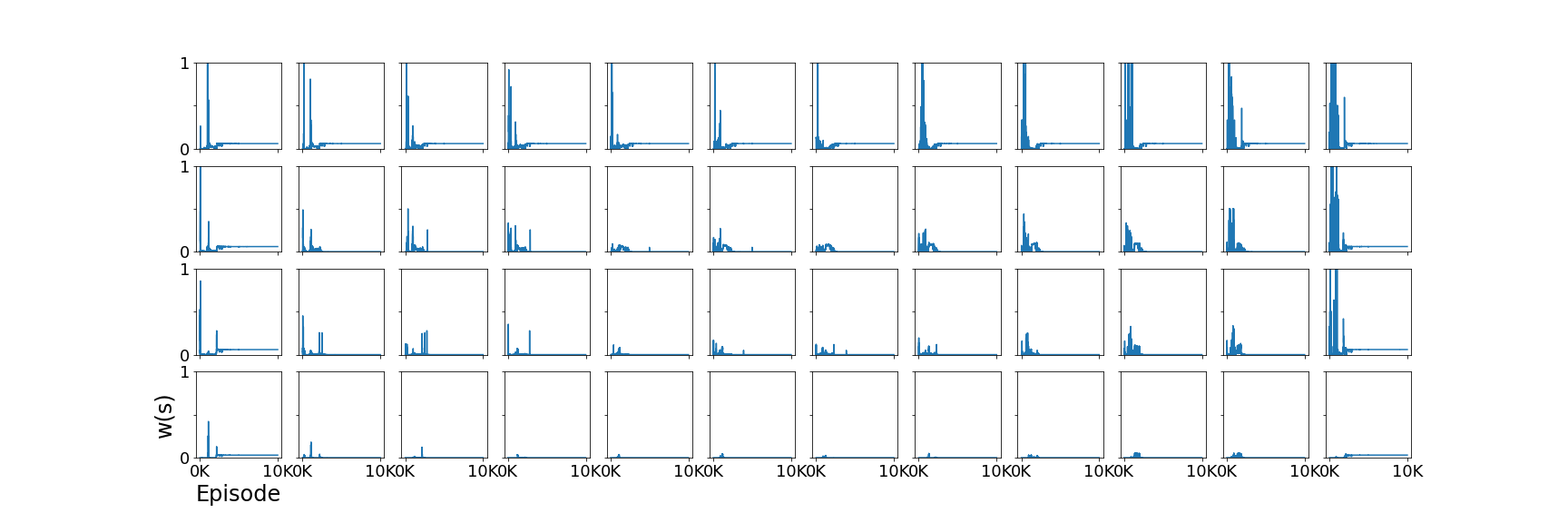
Figure 4: Learned state distribution correction $w(s)$ over 10k training episodes from the $\alpha=0.25$ policy in the stochastic Cliffwalk in Figure 2. Each square corresponds to one state in the grid, e.g. the start state is on the bottom left.

Learned Lagrangian Variables.

The $\xi_{s}(s^{\prime})$ for the $\alpha=0.25$ policy in the stochastic Cliffwalk from Figure 2 is shown in Figure 5 for each of the $4\times 12$ Cliffwalk states. For the start state (bottom left grid), initially $\xi_{s_{0}}(s_{\text{cliff}})$ corresponding to walking right and falling into the cliff is high. After the policy learns a deterministic path around 3-4K episodes, the $\xi_{s}(s^{\prime})$ corresponding to the deterministic transition $s^{\prime}$ such that $P_{\theta}(s^{\prime}|s)=1$ for each $s$ must also be 1 due to the constraint that $E_{P_{\theta}}[\xi]=1$. For $s^{\prime}$ where $P_{\theta}(s^{\prime}|s)=0$, the $\xi_{s}(s^{\prime})$ are free variables and do not affect the value.

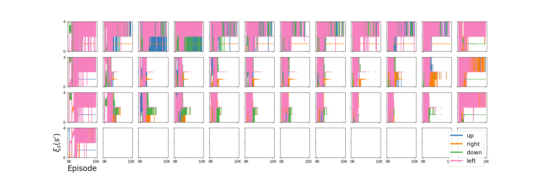
Figure 5: Learned state distribution correction $\xi_{s}(s^{\prime})$ over 10k training episodes from the $\alpha=0.25$ policy in the stochastic Cliffwalk in Figure 2. Each square corresponds to one state in the grid, e.g. the start state is on the bottom left. For each state $s$, the color of the line corresponds to next state $s^{\prime}$ resulting from each of the 4 actions taken (see legend).

C.4 Function Approximation for $w,\xi,\lambda$

Finally, in Algorithm 3 we present a method for learning $w,\xi,\lambda$ in the function approximation setting, such as large or continuous state spaces, where the use of convex solvers may become difficult. In such cases, $w$ and $\xi,\lambda$ can be learned using neural networks for a total of five networks–the actor, critic, $w$, $\xi$, and $\lambda$. For $\text{CVaR}_{\alpha}$, for example, only $\lambda^{P}$ needs to be learned since the constraint that $\xi\in[0,\frac{1}{\alpha}]$ can naturally be implemented by using a Softmax activation in the final layer of the $\xi$ network, and multiplying the output by $\frac{1}{\alpha}$. The $\lambda^{P}$ network controls the constraint that $\mathbb{E}_{P_{\theta}}[\xi]=1$.

The $w$ network seeks to minimize $L(w,f)$ in Theorem 6.1, an algorithm for which is given in Algorithm 2 of Liu et al. [2018]. In practice, for discrete state spaces the delta kernel can be used for $f$, and in continuous state spaces an RBF kernel with radius set to be the median of distances between states in the batch can be used for $f$ [Liu et al., 2020]. The $\xi,\lambda$ networks seek to maximize and minimize the MCR objective (4.1), respectively. The gradients of the MCR objective with respect to $\xi$ and $\lambda$ are given in Lemma C.2. We recommend that a higher learning rate is using for the $\lambda$ network and a lower learning rate is used for the $\xi$ network. The Lagrangian can be cast as a two-player zero sum game with a bilinear term between $\xi$ and $\lambda$, and min-max gradient descent for such objectives has been proven to converge only with finite timescale separation [Fiez and Ratliff, 2020]. We do not include experiments as it is beyond the scope of our paper, but hope that algorithms such as Algorithm 3 can serve as a basis for future work in scaling coherent risk policy gradient algorithms to larger or continuous state spaces.

Input: Risk envelope $\mathcal{U}$, learning rates $\{\eta_{w},\eta_{c},\eta_{\xi},\eta_{\lambda},\eta\}$, batch sizes $\{B_{w},B_{c},B_{l}\}$, updates $\{N_{w},N_{c},N_{l}\}$.

Initialize: Policy network $\theta$, critic network $\theta_{c}$, $w$ network $\theta_{w}$, $\xi$ network $\phi$, $\lambda$ network $\psi$;

for episode $k=1...K$  do

       Generate $N$ trajectories $\tau_{k}=\{s_{0}^{(n)},a_{0}^{(n)},c_{0}^{(n)},...\}_{n=1}^{N}$ using $\pi_{\theta}$;

       Pad $\tau_{k}$ if necessary;

       for state ratio updates $i=1...N_{w}$ do

             Sample a minibatch $B_{w}\sim\tau_{k}$;

             Perform one update to $\theta_{w}$ according to Algorithm 4 with stepsize $\eta_{w}$;

            

       end for

      for critic updates $i=1...N_{c}$ do

             Sample a minibatch $B_{c}\sim\tau_{k}$;

             Calculate $l_{\theta_{c}}=\frac{1}{|B_{c}|}\sum_{(s,s^{\prime})\sim B_{c}}\bigg{(}V_{\theta_{c}}(s)-\Big{(}C(s)+L_{\theta,s}(\xi_{\phi},\lambda_{\psi})\Big{)}\bigg{)}^{2}$ with $L_{\theta,s}$ from (5);

             $\theta_{c}\leftarrow\theta_{c}+\eta_{c}\frac{\partial l_{\theta_{c}}}{\partial\theta_{c}}$;

            

       end for

      for $\xi,\lambda$ updates $i=1...N_{l}$ do

             Sample a minibatch $B_{l}\sim\tau_{k}$;

             Calculate gradients $\frac{\partial V}{\partial\theta_{\xi}}$ and $\frac{\partial V}{\partial\theta_{\xi}}$ according to Lemma C.2;

             $\theta_{\xi}\leftarrow\theta_{\xi}+\eta_{\xi}\frac{\partial V}{\partial\theta_{\xi}}$;

             $\theta_{\lambda}\leftarrow\theta_{\lambda}+\eta_{\lambda}\frac{\partial V}{\partial\theta_{\lambda}}$;

            

       end for

      Compute $\widehat{h}(s,a)$ in (4.1);

       Compute $\nabla_{\theta}V_{\theta}=\sum_{s,a,s^{\prime}\sim\tau_{k}}w_{\theta_{w}}(s)\nabla_{\theta}\log\pi_{\theta_{k}}(a|s)\widehat{h}(s,a)$;

       Update $\theta\leftarrow\theta-\eta\nabla_{\theta}V_{\theta}$;

      

end for

Algorithm 3 Stationary State Distribution Reweighting Actor-Critic with Function Approximation

Input: $w$ network parameters $\theta_{w}$, learning rate $\eta_{w}$, batch of transitions $B_{w}$, weightings $\xi$, discount factor $\gamma\in(0,1]$, kernel $k$.

Compute $\widehat{L}(w)=\frac{1}{|B_{w}|}\sum_{i,j\in B_{w}}\Delta(w;s_{i},s_{i}^{\prime})\Delta(w;s_{j},s_{j}^{\prime})k(s_{i}^{\prime},s_{j}^{\prime})$;

where $\Delta(w,s,s^{\prime})=w(s)\xi_{s}(s^{\prime})-w(s^{\prime})$.;

Update the parameter by $\theta_{w}\leftarrow\theta_{w}-\eta_{w}\nabla_{\theta}\widehat{L}(w_{\theta_{w}}/z_{w_{\theta_{w}}})$;

where $z_{w_{\theta_{w}}}$ is a normalization constant $z_{w_{\theta_{w}}}=\frac{1}{|B_{w}|}\sum_{i\in B_{w}}w_{\theta_{w}}(s_{i})$. ;

Algorithm 4 Single $w$ Update (adapted from Algorithm 2 in Liu et al. [2018])

Lemma C.2 (Gradient of MCR w.r.t $\xi,\lambda$. ).

Let the policy network be parameterized by $\theta$, the $\xi$-network parameterized by $\phi$, and the $\lambda$-network be parameterized by $\psi$. Then the gradient of the objective $V_{\theta,\phi,\psi}$ with respect to $\phi$ is

$$\nabla_{\phi}V_{\theta,\phi,\psi}(s)=\mathbb{E}_{\xi_{\phi}}\bigg{[}\sum_{t=0}^{\infty}\gamma^{t}h_{\phi}(s_{t})|s_{0}=s;\pi_{\theta}\bigg{]}$$ (24)

where

$$h_{\phi}(s)=\gamma\sum_{s^{\prime}}P_{\theta}(s^{\prime}|s)\nabla_{\phi}\xi_{\phi}(s^{\prime}|s)\bigg{(}V_{\theta,\phi,\psi}(s^{\prime})-\lambda_{\psi}(p|s)-\sum_{e}\lambda_{\psi}(e|s)\frac{dg_{e}(\xi_{\phi},P_{\theta})}{d\xi(s^{\prime})}-\sum_{i}\lambda_{\psi}(i|s)\frac{df_{i}(\xi_{\phi},P_{\theta})}{d\xi(s^{\prime})}\bigg{)}$$ (25)

The gradient with respect to $\psi$ is

$$\nabla_{\psi}V_{\theta,\phi,\psi}(s)=\mathbb{E}_{\xi_{\phi}}\bigg{[}\sum_{t=0}^{\infty}\gamma^{t}h_{\psi}(s_{t})|s_{0}=s;\pi_{\theta}\bigg{]}$$ (26)

where

$$h_{\psi}(s)=-\gamma\bigg{(}\nabla_{\psi}\lambda_{\psi}(p|s)\Big{(}\sum_{s_{1}}P_{\theta}(s^{\prime}|s)\xi_{\psi}(s^{\prime}|s)-1\Big{)}+\sum_{e}\nabla_{\psi}\lambda_{\psi}(e|s)g_{e}(\xi_{\phi},P_{\theta})+\sum_{i}\nabla_{\psi}\lambda_{\psi}(i|s)f_{i}(\xi_{\phi},P_{\theta})\bigg{)}$$ (27)

Proof.

The proof follows from applying the chain rule to the Lagrangian formulation of the objective (5) using the same techniques as the proof of Theorem 4.1 in Appendix A. ∎

References

• Acerbi (2002) Carlo Acerbi. Spectral measures of risk: A coherent representation of subjective risk aversion. Journal of Banking & Finance, 26(7):1505–1518, 2002.
• Agarwal et al. (2019) Alekh Agarwal, Sham M. Kakade, Jason D. Lee, and Gaurav Mahajan. On the theory of policy gradient methods: Optimality, approximation, and distribution shift, 2019.
• Agrawal et al. (2018) Akshay Agrawal, Robin Verschueren, Steven Diamond, and Stephen Boyd. A rewriting system for convex optimization problems. Journal of Control and Decision, 5(1):42–60, 2018.
• Alexander et al. (2006) Siddharth Alexander, Thomas F Coleman, and Yuying Li. Minimizing cvar and var for a portfolio of derivatives. Journal of Banking & Finance, 30(2):583–605, 2006.
• Artzner et al. (1999) Philippe Artzner, Freddy Delbaen, Jean-Marc Eber, and David Heath. Coherent measures of risk. Mathematical finance, 9(3):203–228, 1999.
• Azizzadenesheli et al. (2018) Kamyar Azizzadenesheli, Yisong Yue, and Animashree Anandkumar. Policy gradient in partially observable environments: Approximation and convergence. arXiv e-prints, pages arXiv–1810, 2018.
• Beck (2017) Amir Beck. First-order methods in optimization. SIAM, 2017.
• Bellemare et al. (2017) Marc G Bellemare, Will Dabney, and Rémi Munos. A distributional perspective on reinforcement learning. arXiv preprint arXiv:1707.06887, 2017.
• Bhandari and Russo (2019) Jalaj Bhandari and Daniel Russo. Global optimality guarantees for policy gradient methods. arXiv preprint arXiv:1906.01786, 2019.
• Chow and Ghavamzadeh (2014) Yinlam Chow and Mohammad Ghavamzadeh. Algorithms for cvar optimization in mdps. In Advances in neural information processing systems, pages 3509–3517, 2014.
• Chow et al. (2015) Yinlam Chow, Aviv Tamar, Shie Mannor, and Marco Pavone. Risk-sensitive and robust decision-making: a cvar optimization approach. In Advances in Neural Information Processing Systems, pages 1522–1530, 2015.
• Di Castro et al. (2012) Dotan Di Castro, Aviv Tamar, and Shie Mannor. Policy gradients with variance related risk criteria. arXiv preprint arXiv:1206.6404, 2012.
• Diamond and Boyd (2016) Steven Diamond and Stephen Boyd. CVXPY: A Python-embedded modeling language for convex optimization. Journal of Machine Learning Research, 17(83):1–5, 2016.
• Fei et al. (2020) Yingjie Fei, Zhuoran Yang, Yudong Chen, Zhaoran Wang, and Qiaomin Xie. Risk-sensitive reinforcement learning: Near-optimal risk-sample tradeoff in regret, 2020.
• Fiez and Ratliff (2020) Tanner Fiez and Lillian Ratliff. Gradient descent-ascent provably converges to strict local minmax equilibria with a finite timescale separation, 2020.
• Garcıa and Fernández (2015) Javier Garcıa and Fernando Fernández. A comprehensive survey on safe reinforcement learning. Journal of Machine Learning Research, 16(1):1437–1480, 2015.
• Ghadimi and Lan (2016) Saeed Ghadimi and Guanghui Lan. Accelerated gradient methods for nonconvex nonlinear and stochastic programming. Mathematical Programming, 156(1-2):59–99, 2016.
• Keramati et al. (2019) Ramtin Keramati, Christoph Dann, Alex Tamkin, and Emma Brunskill. Being optimistic to be conservative: Quickly learning a cvar policy. arXiv preprint arXiv:1911.01546, 2019.
• Liu et al. (2018) Qiang Liu, Lihong Li, Ziyang Tang, and Dengyong Zhou. Breaking the curse of horizon: Infinite-horizon off-policy estimation. arXiv preprint arXiv:1810.12429, 2018.
• Liu et al. (2020) Yao Liu, Adith Swaminathan, Alekh Agarwal, and Emma Brunskill. Off-policy policy gradient with stationary distribution correction. In Uncertainty in Artificial Intelligence, pages 1180–1190. PMLR, 2020.
• Mavrin et al. (2019) Borislav Mavrin, Shangtong Zhang, Hengshuai Yao, Linglong Kong, Kaiwen Wu, and Yaoliang Yu. Distributional reinforcement learning for efficient exploration. arXiv preprint arXiv:1905.06125, 2019.
• Milgrom and Segal (2002) Paul Milgrom and Ilya Segal. Envelope theorems for arbitrary choice sets. Econometrica, 70(2):583–601, 2002.
• Pflug and Pichler (2016) Georg Ch Pflug and Alois Pichler. Time-consistent decisions and temporal decomposition of coherent risk functionals. Mathematics of Operations Research, 41(2):682–699, 2016.
• Prashanth and Ghavamzadeh (2013) LA Prashanth and Mohammad Ghavamzadeh. Actor-critic algorithms for risk-sensitive mdps. In Advances in neural information processing systems, pages 252–260, 2013.
• Prashanth et al. (2016) LA Prashanth, Cheng Jie, Michael Fu, Steve Marcus, and Csaba Szepesvári. Cumulative prospect theory meets reinforcement learning: Prediction and control. In International Conference on Machine Learning, pages 1406–1415, 2016.
• Ruszczyński (2010) Andrzej Ruszczyński. Risk-averse dynamic programming for markov decision processes. Mathematical programming, 125(2):235–261, 2010.
• Ruszczyński and Shapiro (2006) Andrzej Ruszczyński and Alexander Shapiro. Optimization of convex risk functions. Mathematics of operations research, 31(3):433–452, 2006.
• Shapiro et al. (2009) A Shapiro, D Dentcheva, and A Ruszczynski. Lectures on stochastic programming: Modeling and theory, mos-siam ser. Optim., SIAM, Philadelphia, 2009.
• Sutton and Barto (2018) Richard S Sutton and Andrew G Barto. Reinforcement learning: An introduction. MIT press, 2018.
• Tamar et al. (2015a) Aviv Tamar, Yinlam Chow, Mohammad Ghavamzadeh, and Shie Mannor. Policy gradient for coherent risk measures. In Advances in Neural Information Processing Systems, pages 1468–1476, 2015a.
• Tamar et al. (2015b) Aviv Tamar, Yonatan Glassner, and Shie Mannor. Optimizing the cvar via sampling. In Proceedings of the Twenty-Ninth AAAI Conference on Artificial Intelligence, pages 2993–2999, 2015b.