On accelerating a multilevel correction adaptive finite element method for Kohn-Sham equation111This research is supported partly by National Key R&D Program of China 2019YFA0709600, 2019YFA0709601, National Natural Science Foundations of China (Grant Nos. 11801021, 11922120, 11871489 and 11771434), MYRG of University of Macau (MYRG2019-00154-FST) and the National Center for Mathematics and Interdisciplinary Science, CAS.
Abstract
Based on the numerical method proposed in [G. Hu, X. Xie, F. Xu, J. Comput. Phys., 355 (2018), 436–449.] for Kohn-Sham equation, further improvement on the efficiency is obtained in this paper by i). designing a numerical method with the strategy of separately handling the nonlinear Hartree potential and exchange-correlation potential, and ii). parallelizing the algorithm in an eigenpairwise approach. The feasibility of two approaches are analyzed in detail, and the new algorithm is described completely. Compared with previous results, a significant improvement of numerical efficiency can be observed from plenty of numerical experiments, which make the new method more suitable for the practical problems.
Keywords. Kohn-Sham equation, multilevel correction method, finite element method, separately handing nonlinear terms, parallel computing. AMS subject classifications. 65N30, 65N25, 65L15, 65B99.
1 Introduction
Kohn-Sham Density functional theory (DFT) is one of the most successful approximate models in the study of many-body system. Its application has covered many practical application areas , ranging from chemistry, physics, materials science, chemical engineering, etc. With rapid development of the hardware, new algorithms and acceleration techniques are desired to keep improving the efficiency of the simulations in density functional theory.
So far, lots of numerical methods for solving Kohn-Sham equation have been developed. For instance, plane-wave method is the most popular method in the computational quantum chemistry community. Owing to the independence of the basis function to the ionic position, plane-wave method has advantage on calculating intermolecular force. Combined with the pseudopotential method, plane-wave method plays an important role in the study of the ground and excited states calculations, and geometry optimization of the electronic structures. Although the plane-wave method is popular in the computational quantum chemistry community, it is inefficient in the treatment of non-periodic systems like molecules, nano-clusters, etc., or materials systems with defects, where higher basis resolution is often required in some spatial regions and a coarser resolution suffices elsewhere. Furthermore, the plane-wave method uses the global basis which significantly affect the scalability of computations on parallel computing platforms. The atomic-orbital-type basis sets [16, 19, 42] are also widely used for simulating materials systems such as molecules and clusters. However, they are well suited only for isolated systems with special boundary conditions. It is difficult to develop a systematic basis-set for all materials systems. Thus over the past decade, more and more attention have been attracted to develop efficient and scalable real-space techniques for electronic structure calculations. For more information, we refer to [5, 6, 9, 10, 15, 28, 35, 36] and references therein for a comprehensive overview.
Among all those real-space methods for Kohn-Sham equation, the finite element method is a very competitive one. The advantages of finite element method for solving the partial differential equations include that it can use unstructured meshes and local basis sets, and it is scalable on parallel computing platforms. So far, the application of the finite element method on solving Kohn-Sham equation has been studied systematically. Please refer to [3, 7, 14, 17, 23, 24, 27, 30, 31, 32, 34, 37, 38, 39, 40, 41, 47], and references therein.
Efficiency improvement is a key issue in the development of the method towards the practical simulations. Many acceleration techniques such as adaptive mesh methods, multigrid preconditioning in solving the eigenvalue problems, parallelization, have been studied in depth for the purpose. It is noted that Xie and his co-workers proposed and developed a multilevel correction technique for solving eigenvalue problems [12, 20, 25, 43, 44, 45]. With this technique, solving the nonlinear eigenvalue problem defined on the finest mesh can be transformed to solving the linear boundary value problem on the finest mesh and a fixed and low dimensional nonlinear eigenvalue problem. Fruitful results have been obtained to successfully show the capability of the multilevel correction method on improving the efficiency. In [18], a numerical framework consisting of the multilevel correction method and the -adaptive mesh method is proposed for solving the Kohn-Sham equation. Similar to original idea of the multilevel correction method, the nonlinear eigenvalue problem derived from the finite element discretization of the Kohn-Sham equation is fixed in a relatively coarse mesh, while the finite element space built on this coarse mesh is kept enriching by the solutions from a series of boundary value problems derived from the Kohn-Sham equation. Here the -adaptive mesh method is used to tailor a fitting nonuniform mesh for the derived boundary value problem, so that the finite element space for the nonlinear eigenvalue problem can be improved well. The performance of proposed solver for the Kohn-Sham equation has been checked by the following works [12, 18, 20, 44, 45].
In this paper, the efficiency of the proposed numerical method in [18] will be further improved, based on following two approaches. The first approach is based on an observation of significant difference of contributions for total energy of the system from two nonlinear terms in the hamiltonian, i.e., Hartree potential and exchange-correlation potential. It is the nonlinearity introduced by these two potentials which makes the analysis and calculation of Kohn-Sham equation nontrivial. Unlike the Hartreen potential which has an exact expression, there is no exact expression for the exchange-correlation potential. Hence, an approximation such as local density approximation (LDA) is needed for the study. An interesting observation for the difference between Hartree and exchange-correlation potentials can be made, based on following results from NIST standard reference database 141 [21].
| E_tot | E_kin | E_har | E_coul | E_xc |
| -847.277 | 846.051 | 355.232 | -2008.741 | -39.319 |
It is clearly seen that the magnitude of the exchange-correlation energy (E_xc) is just around 10% of the Hartree energy (E_har). It also should be noted that similar comparisons exist for all other elements in the period table. Such observation brings us a chance to further improve the efficiency of the algorithm by separately considering two nonlinear terms. The idea is to reduce the computational resource for handling the nonlinearity introduced by the Hartree potential. which is realized by designing a new iteration scheme to replace the traditional self-consistent field iteration scheme in this paper. The new scheme consists of two nested iteration schemes, i.e., an outer iteration for resolving the nonlinearity from the exchange-correlation potential, and an inner iteration for resolving the nonlinearity from the Hartree potential. Although there are two iterations in our algorithm, it is noted that the outer iteration process for the nonlinearity of the exchange-correlation term always be done around 10 times in our numerical experiments for molecules from a lithium hydride (2 atoms) to a sodium cluster (91 atoms). For the inner iteration, dozens of iterations are needed in each outer iteration at the beginning. However, with the increment of the outer iterations, the number of the inner iterations decreases significantly. Hence, the total number of the iterations (inner iterations by outer iterations) of our method is fairly comparable with that of a standard SCF iteration. However, due to the separation of two nonlinear terms and the framework of multilevel correction method, the calculation involving the basis function defined on the fine mesh can be extracted separately and precalculated, so that the computational work of the inner iteration only depends on the dimension of the coarse space. With this strategy, a large amount of CPU time can be saved in the simulations, compared with the original multilevel correction method [18].
To further improve the efficiency, the eigenpairwise parallelization of the algorithm based on message passing interface (MPI) is also studied in this work. One desired feature for the algorithm is an wavefunction-wise parallelization, based on which the calculation can be done for each wavefunction separately, and a significant acceleration for the overall simulation can be expected. However, this is quite nontrivial for a problem containing eigenvalue problem because of the possible orthogonalization for all wavefuntions needed during the simulation. One attractive feature of multilevel correction method is that the wavefunction-wise parallelization can be partially realized in the sense that the correction of the wavefunction can be done individually in the inner iteration. In this work, we have redesigned the algorithm to fully take advantage of this feature. It is worth to rementioning another feature of the multilevel correction method is that the eigenvalue problem is solved on the corasest mesh, which can be solved effectively. By combining these two strategies, a dramatic acceleration for the simulation can be observed clearly from the numerical experiments.
The outline of this paper is as follows. In Section 2, we recall the multilevel correction adaptive finite element method for solving Kohn-Sham equation. In Section 3, we construct an accelerating multilevel correction adaptive finite element method which can further improve the solving efficiency for Kohn-Sham equation. In Section 4, some numerical experiments are presented to demonstrate the efficiency of the presented algorithm. Finally, some concluding remarks are presented in the last section.
2 Multilevel correction adaptive finite element method for Kohn-Sham equation
In this section, we review the multilevel correction adaptive finite element method for Kohn-Sham equation (see [18]). To describe the algorithm, we introduce some notation first. Following [1], we use to denote Sobolev spaces, and and to denote the associated norms and seminorms, respectively. In case , we denote and , where is in the sense of trace, and denote . In this paper, we set for simplicity.
Let be the Hilbert space with the inner product
| (1) |
where in this paper. For any and a subdomain , we define and
Let be a subspace of with orthonormality constraints:
| (2) |
where .
We consider a molecular system consisting of nuclei with charges , , and locations , , , respectively, and electrons in the non-relativistic and spin-unpolarized setting. The general form of Kohn-Sham energy functional can be demonstrated as follows
| (3) |
for . Here, is the Coulomb potential defined by , is the electron-electron Coulomb energy (Hartree potential) defined by
| (4) |
and is some real function over denoting the exchange-correlation energy.
The ground state of the system is obtained by solving the minimization problem
| (5) |
and we refer to [11, 8] for the existence of a minimizer under some conditions.
The Euler-Lagrange equation corresponding to the minimization problem (5) is the well known Kohn-Sham equation: Find such that
| (6) |
where is the Kohn-Sham Hamiltonian operator as
| (7) |
with and . The variational form of the Kohn-Sham equation can be described as follows: Find such that
| (8) |
In the ground state of the electronic system, electrons will occupy the orbitals with the lowest energies. Hence, it corresponds to finding the left most eigenpairs of Kohn-Sham equation. If the spin polarization is considered, the number of the eigenpairs is the same to the number of the electrons. Otherwise, only half eigenpairs are needed. For simplicity, we only consider the spin-unpolarized case in this paper.
In order to define an efficient way to treat the nonlinear Hartree potential term, we introduce the mixed formulation of the Kohn-Sham equation. It has been observed from the numerical practice that the term provides the main nonlinearity, where is the Hartree (electrostatic) potential and its analytical form can be obtained by solving the following Poisson equation:
| (9) |
with a proper Dirichlet boundary condition.
Now, let us define the finite element discretization of (23). First we generate a shape regular decomposition of the computing domain and let denote the interior edge set of . The diameter of a cell is denoted by and the mesh diameter describes the maximum diameter of all cells . Based on the mesh , we construct the linear finite element space denoted by . Define and it is obvious that .
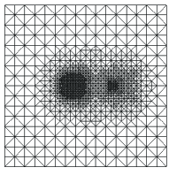
In order to recover the singularity of Kohn-Sham equation, the adaptive finite element method (AFEM) is the standard way. With the adaptive mesh refinement guided by the a posteriori error estimators, the AFEM can produce an efficient discretization scheme for the singular problems. The total amount of the mesh elements should be controlled well to make the simulation continuable and efficient for the Kohn-Sham equation. Based on the above discussion, adaptive mesh method is a competitive candidate for the refinement strategy. A standard AFEM process can be described by the following way
Solve Estimate Mark Refine.
More precisely, to get from , we first solve the discrete equation on to get the approximate solution and then calculate the a posteriori error estimator on each mesh element. Next we mark the elements with big errors and these elements are refined in such a way that the triangulation is still shape regular and conforming.
In our simulation, the residual type a posteriori error estimation is employed to generate the error indicator. First, we construct the element residual and the jump residual for the eigenpair approximation as follows:
| (11) | |||
| (12) |
where is the common side of elements and with the unit outward normals and , respectively. Let be the set of interior faces (edges or sides) of , and be the union of element sharing a side with . For , we define the local error indicator by
| (13) |
Given a subset , we define the error estimate by
| (14) |
Based on the error indicator (14), we use the Dörfler’s marking strategy [13] to mark all elements in for local refinement.
Since solving large-scale nonlinear eigenvalue problem is quite time-consuming compared to that of boundary value problem, a multilevel correction adaptive method for solving Kohn-Sham equation was designed in [18, Algorithms 1 and 3]. The multilevel correction method transforms solving Kohn-Sham equation on the adaptive refined mesh to the solution of the associated linear boundary value problems on and nonlinear eigenvalue problem in a fixed low dimensional subspace which is build with the finite element space on the coarse mesh and finite element functions . In the multilevel correction adaptive method for solving Kohn-Sham equation, we need to solve linear boundary value problems in each adaptive space and a small-scale Kohn-Sham equation in the correction space . Since there is no eigenvalue problem solving in the fine mesh , the multilevel correction adaptive method has a better efficiency than the direct AFEM. The dimension of the correction space is fixed and small in the multilevel correction adaptive finite element method. But we need to solve a nonlinear eigenvalue problem in the correction space . Always, some type of nonlinear iteration steps are required to solve this nonlinear eigenvalue problems. When the system includes large number of electrons, the number of required nonlinear iteration steps is always very large. Furthermore, the correction space contains basis functions defined in the fine space . In order to guarantee the calculation accuracy, we need to assemble matrices in the fine space when it comes to the basis functions of defined on the fine mesh . This part of work depends on the number of electrons and dimension of as . In order to improve the efficiency of the correction step, a new type of nonlinear iteration method and an eigenpairwise parallel correction method with efficient implementing techniques will be designed in the next section.
3 Further improvement of the method towards the efficiency
In this section, we give a new type of AFEM which is a combination of the multilevel correction scheme, nonlinearity separating technique and an efficient parallel method for the Hartree potential. The nonlinearity separating technique is designed based on the different performance of the exchange-correlation and Hartree potentials. We will use the self consistent field (SCF) iteration steps to treat the weak nonlinear exchange-correlation potential and the multilevel correction method for the strong nonlinear Hartree potential. Furthermore, combining the eigenpairwise parallel idea from [46] and the special structure of the Hartree potential, the Hartree potential can be treated by the parallel way and an efficient implementing technique.
3.1 A strategy of separating nonlinear terms
The nonlinearity of the Kohn-Sham equation comes from Hartree and exchange-correlation potentials. As discussed in Section 1, the Hartree potential has a strong nonlinearity which leads the main nonlinearity of the Kohn-Sham equation, while the nonlinearity of the exchange-correlation potential is weak. Based on such a property, we modify the standard SCF iteration into a nested iteration which includes outer SCF iteration for the exchange-correlation potential, and inner multilevel correction iteration for the Hartree potential. Furthermore, we will also design an eigenpairwise parallel multilevel correction method for solving the nonlinear eigenvalue problems associated with the Hartree potential in the inner iterations.
Actually, this section is to define an efficient numerical method to solve the Kohn-Sham equation on the refined mesh with the proposed nested iteration here. Different from the standard SCF iteration, we decompose the SCF iteration into outer iteration for exchange-correlation potential and inner iteration for the Hartree potential. This type of nonlinear treatment is based on the understanding of the nonlinearity strengthes from the Hartree and exchange-correlation potentials, respectively. In the practical models and computing experience, the nonlinearity of Hartree Potential is stronger than that of the exchange-correlation potential.
Given an initial value for the Kohn-Sham equation, we should solve the following nonlinear eigenvalue problem in each step of the outer SCF iteration method for the exchange-correlation potential: For , find such that
| (16) |
where
| (18) |
and
| (19) |
In the above SCF iteration, only the exchange-correlation potential is linearized. Thus, we still need to solve a nonlinear eigenvalue problem in each iteration step, and the nonlinearity is caused by the Hartree potential. Because the nonlinearity of the exchange-correlation potential is weak, so only a few steps are needed for the above SCF iteration. Further, for the involved nonlinear eigenvalue problem whose nonlinearity is caused by the Hartree potential, we can design a new strategy to solve it efficiently.
It is obvious that equation (16) is still a nonlinear eigenvalue problem with the nonlinear term of Hartree potential. Now, we spend the main attentions to design an efficient eigenpairwise parallel way to solve the nonlinear eigenvalue problem (16). The idea and method here come from [18, 46, 48]. This type of method is built based on the low dimensional space defined on the coarse mesh . But the method in this paper is the eigenpairwise parallel way to implement the augmented subspace method which is different from [18]. Compared with the standard SCF iteration method for Kohn-Sham equation, there is no inner products for orthogonalization process in the high dimensional space , which is always the bottle neck for parallel computing.
In order to define the eigenpairwise multilevel correction method for the Hartree potential, we transform the Kohn-Sham equation (8) into the following equivalently mixed form: Find such that
| (23) |
where the function set is defined by the trace of Hartree potential on the boundary
In the practical computation, the discrete form of (23) can be described as follows: Find such that
| (27) |
where the set includes linear finite element functions with the boundary condition which is computed by the fast multipole method [3, (29)].
The corresponding scheme is defined by Algorithm 1, where we can find that the augmented subspace method transforms solving the nonlinear eigenvalue problem into the solution of the boundary value problem and some small scale nonlinear eigenvalue problems in the low dimensional space .
| (29) |
| (30) |
| (31) |
The linear boundary value problems (29) and (30) in Algorithm 1 are easy to be solved by the efficient and matured linear solvers. For example, the linear solvers based on the multigrid method always give the optimal efficiency for solving the second order elliptic problems. Compared with the multilevel correction method defined in [18], the obvious difference is that Algorithm 1 treats the different orbit associated with , , indepdently. This way can avoid doing inner products for orthogonalization in the high dimensional space . Furthermore, we will design an efficient numerical method for solving the nonlinear eigenvalue problem (31) with a special implemenmting techqniue in the next subsection.
3.2 New algorithm and its parallel implementation
In this subsection, we further study two important characteristics of Algorithm 1, which will help to accelerate the solving efficiency. The first characteristic is that the SCF iteration for the nonlinear eigenvalue problem (31) can be implemented efficiently. The idea here comes from [46, 48]. The second characteristic is that Algorithm 1 is suitable for eigenpairwise parallel computing.
We begin with the first characteristic of Algorithm 1 by introducing an efficient implementation of the iteration method for the nonlinear eigenvalue problem (31). The corresponding implementation scheme is described by Algorithm 2.
-
(a).
For , solve the following linear eigenvalue problem.
(32) Solve ((a).) and choose the eigenfunction that has the largest component in span among all the eigenfunctions.
-
(b).
Solve the following elliptic problem: Find such that
(33) -
(c).
If , stop the iteration. Else set and go to (a) to do the next iteration step.
Different from the standard SCF method, the one in Algorithm 2 use the mixed form of Kohn-Sham equation to do the nonlinear iteration. Even the mixed form is equivalent to the standard one, it provides a chance to design an efficient implementing way to do the nonlinear iteration. This means the remaining part of this subsection is to discuss how to perform Algorithm 2 efficiently based on the special structure of the correction spaces and . The designing process for the efficient implementing way also shows a reason to treat the Hartree potential and exchange-correlation potential separately.
From the definition of Algorithm 2, we can find that solving eigenvalue problem ((a).) and linear boundary value problem (33) need very small computation work since the dimensions of and are very small. But both and include finite element functions defined on the finer mesh . In order to guarantee the accuracy, we need to assemble the matrices and right hand side terms in ((a).) and (33) in the finer mesh which needs the computational work . Based on this consideration, the key point for implementing Algorithm 2 efficiently is to design an efficient way to assemble the concerned matrices and right hand side terms. For the description of implementing technique here, let denotes the Lagrange basis function for the coarse finite element space .
In order to show the main idea here, let us consider the matrix version of eigenvalue problem ((a).) as follows
| (34) |
where , , and , , .
Since it is required to solve linear eigenvalue problems which can be assembled in the same way, we use and to denote and , respectively, for simplicity. We should know that the following process is performed for each SCF iteration. Here, for readability, the upper indices used in our algorithm is also omitted.
It is obvious that the matrix , the vector and the scalar will not change during the nonlinear iteration process as long as we have obtained the function . But the matrix , the vector and the scalar will change during the nonlinear iteration process. Then it is required to consider the efficient implementation to update the the matrix , the vector and the scalar since there is a function which is defined on the fine mesh . The aim here is to propose an efficient method to update the matrix , the vector and the scalar without computing on the fine mesh during the nonlinear iteration process. Assume we have a given initial value for Hartree potential. Now, in order to carry out the nonlinear iteration for the eigenvalue problem (34), we come to consider the computation for the matrix , the vector and the scalar .
From the definitions of the space and the eigenvalue problem ((a).), the matrix has the following expansion
| (35) | |||||
Here , remain unchanged during the inner nonlinear iteration. During the inner loop, the exchange-correlation potential remains unchanged, so the matrix also remains unchanged during the inner nonlinear iteration. Thus we can assemble , , in advance, and call these data directly in each iteration step. The matrix will change during the nonlinear iteration because will change. But is defined on the coarse space , which can be assembled by the small computational work .
The vector has the following expansion
| (36) | |||||
Because is a basis function of the correction space , so remain unchanged during the inner nonlinear iteration. So we can compute these three vectors in advance. In order to compute , we first assemble a matrix in the fine space
| (37) |
which will be fixed during the inner nonlinear iteration and can be computed in advance. Let us define , and . Then, .
The scalar has the following expansion
| (38) | |||||
Here , , remain unchanged during the inner nonlinear iteration. In order to compute efficiently, we first assemble a vector in the fine space :
| (39) |
It is obvious that the vector will be fixed during the inner nonlinear iteration and .
Next, we consider the efficient scheme for solving the Hartree potential equation (33). Based on the structure of the space , the matrix version of (33) can be written as follows
| (40) |
where , , , and .
It is obvious that the matrix , the vector and the scalar will not change during the nonlinear iteration process as long as we have obtained the function . So the main task is to assemble the right hand side term . Since the density function is the sum of the square of approximate eigenfunctions, we should do the summation according to the lower index in our description.
For the right hand term of (40), we have
| (41) | |||||
The vector remains unchanged during the inner SCF iteration and is just the vector in (39) assembled for the -th linear boundary value problem. Because will change during the inner nonlinear iteration, so needs to be computed during the iteration. Fortunately, is defined on the coarse space , which only needs the computational work . The vector can be computed in the way , where is the coefficient vector of with respect to the basis functions of .
From the structure of , the scalar has the following expansion
| (42) | |||||
The scalar remains unchanged during the inner nonlinear iteration. In order to assemble and , let us define a matrix and a vector in the following way which remain unchanged during the inner nonlinear iteration:
| (43) |
Then
| (44) |
Remark 3.1.
In (41) and (42), the density function is the square sum of wavefunctions, so we can expand (41) and (42) into three parts, respectively. Each term can be assembled efficiently.
However, this good property can not be used to exchange-correlation potential because the structure of is non-polynomial. For instance, the simplest form , then we can not expand it into different terms due to the fractional power . This is also a reason to use the outer iteration to deal with exchange-correlation potential. Then the exchange-correlation potential remains unchanged during the inner iteration.
In Algorithm 3, based on above discussion and preparation, we define the efficient implementation strategy for Algorithm 2.
-
11.
Preparation for the nonlinear iteration by assembling the following values for each linear boundary value problem:
Nonlinear iteration:
-
(a)
Compute the matrix as in (35). Then
-
(b)
Compute the vector as in (36). Then the vector .
-
(c)
Compute the scalar .
-
(d)
Then solve the eigenvalue problem (34) to get a new eigenfunction and the corresponding eigenvalue .
- (e)
-
(f)
Compute .
-
(g)
Then solve the boundary value problem (40) to get a new Hartree potential and .
-
(h)
If the given accuracy is satisfied, stop the nonlinear iteration. Otherwise, go to step (a) and continue the nonlinear iteration.
Output the eigenfunction and the eigenvalue .
Remark 3.2.
We need to solve a Poisson equation to derive the Hartree potential. However, the Hartree potential does not decay exponentially as the wavefunction. Thus, we can use the multipole expansion to derive a proper Dirichlet boundary condition. The detailed description can be found in [4], etc. To further improve the solving efficiency, in our algorithm, the Dirichlet boundary condition will renew after each outer iteration and remains unchanged in the inner iteration.
In the last of this subsection, we want to emphasize that Algorithm 1 is naturally suitable for eigenpairwise parallel computing due to its special structure. As we can see, Algorithm 1 treats the different orbits independently. This scheme can avoid doing inner products for orthogonalization in the high dimensional space , which is always time-consuming and becomes the bottle neck for parallel computing. Thus parallel computing will benefit from such a strategy through solving different orbits in different processors. During the iteration of Algorithm 1, we only need to transfer the data when it comes to compute the density function, which just needs the wavefunction derived in each processor. So the time spent on data transmission accounts for only a small part of the total computational time. This is why Algorithm 1 is naturally suitable for parallel computing.
4 Numerical results
In this section, we provide several numerical examples to validate the efficiency and scalability of the proposed numerical method in this paper. The numerical examples are carried out on LSSC-IV in the State Key Laboratory of Scientific and Engineering Computing, Chinese Academy of Sciences. Each computing node has two 18-core Intel Xeon Gold 6140 processors at 2.3 GHz and 192 GB memory. For the involved small-scale eigenvalue problems, we adopt the implicitly restarted Lanczos method provided in the package ARPACK [22].
The numerical experiments in this section are implemented for simulating the following five models. The first model is the lithium hydroxide molecule and the complete Kohn-Sham equation is given by
| (45) |
where . In this equation, and electron density , , denote the position of lithium atom and hydrogen atom, and exchange-correlation potential is adopted as with . Since we don’t consider spin polarisation, eigenpairs need to be calculated for this model.
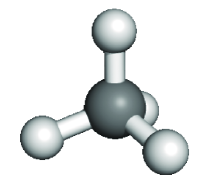
The second model is Methane (CH4) and the computing domain is set to be . The associated parameters in the hamiltonian are the same as the first model. For a full potential calculation, there are total electrons. Since we don’t consider spin polarisation, eigenpairs need to be calculated.
The third model is Acetylene molecule (C2H2). We set the computing domain to be . For a full potential calculation, there are total fourteen electrons. Since we don’t consider spin polarisation, seven eigenpairs need to be calculated. In this model, the local density approximation (LDA) is defined as follows. The exchange energy density is chosen as:
The correlation energy density is chosen as [33]:
with . The exchange-correlation potential is then chosen as
In this model, there are total electrons and we need to compute eigenpairs for the full potential calculation.
The fourth model is Benzene molecule (C6H6) and the computing domain is . The corresponding parameters are the same as the third model with the LDA exchange-correlation potential. There are total electrons. Since we don’t consider spin polarisation, eigenpairs need to be calculated for the full potential calculation.
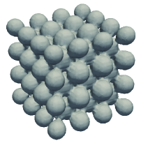
The last model is the body-centered cubic (bcc) structure of Sodium crystal of cubes with atoms. Here, we use the pseudopotential which was introduced in [29] in our numerical experiment and hence valence electrons and eigenpairs are simulated. We use the LDA exchange-correlation potential as that in the third model.
Numerical experiments for these five molecules are implemented to demonstrate following aspects, i.e., the feasibility of spearating nonlinear Hartree potential and exchange-correlation potential in the algorithm, the scalability of the algorithm, as well as the ability of the algorithm on preserving the orthogonality etc. In all numerical examples here, the coarsest mesh for Algorithm 1 is generated by the uniform refinement and includes mesh elements.
4.1 On the feasibility
As mentioned in Introduction, there is significant difference on the contribution for the total ground state energy from Hartree part and exchange-correlation part. Hence, their performance in the convergence towards the ground state should be also different. This can be confirmed by following test.
We consider a lithium hydroxide molecule. To check the convergence behavior with only exchange-correlation potential, governing equation is given below,
| (46) |
where , , , and are the same as in (45).
We use the standard AFEM to solve (46) with the refinement parameter . Table 2 presents the number of SCF iteration times in each level of the adaptive finite element spaces.
For the comparison, we next consider the same molecule, but with only the Hartree potential in the hamiltonian,
| (47) |
Table 3 presents the corresponding number of SCF iteration times in each level of adaptive finite element spaces by the standard AFEM.
| Mesh Level | 1 | 2 | 3 | 4 | 5 | 6 | 7 | 8 | 9 | 10 | 11 | 12 | 13 | 14 | 15 |
| SCF iteration | 07 | 07 | 07 | 07 | 06 | 07 | 07 | 07 | 07 | 06 | 07 | 07 | 07 | 06 | 07 |
| Mesh Level | 1 | 2 | 3 | 4 | 5 | 6 | 7 | 8 | 9 | 10 | 11 | 12 | 13 | 14 | 15 |
| SCF iteration | 23 | 22 | 23 | 22 | 22 | 22 | 23 | 22 | 23 | 22 | 22 | 22 | 22 | 22 | 22 |
From Tables 2 and 3, it can be observed clearly that Hartree potential brings more iterations towards the ground state, compared with exchange-correlation potential. A similar observation is always available for other molecules.
For further understanding the relation of the outer and inner iterations, we solve the lithium hydroxide molecule which is defined by (45). Table 4 presents the numbers of the inner iterations and outer iterations of Algorithm 1 in the final five adaptive finite element spaces. Because the approximate solution obtained from the last outer iteration is used as the initial value, we can see that with approaching the ground state of the molecule, the number of the inner iteration becomes smaller and smaller. Together with the acceleration strategy proposed in Subsection 4.3, the efficiency of proposed algorithm will be improved significantly, compared with the multilevel correction method proposed in [18]. The comparison of the efficiency will be given in following subsections.
| Outer iteration | 1 | 2 | 3 | 4 | 5 | 6 | 7 | 8 |
| Inner iteration | 22 | 17 | 12 | 8 | 5 | 3 | 2 | 0 |
| Outer iteration | 1 | 2 | 3 | 4 | 5 | 6 | 7 | 8 |
| Inner iteration | 20 | 15 | 11 | 8 | 5 | 2 | 2 | 0 |
| Outer iteration | 1 | 2 | 3 | 4 | 5 | 6 | 7 | 8 |
| Inner iteration | 21 | 15 | 12 | 8 | 6 | 3 | 2 | 1 |
| Outer iteration | 1 | 2 | 3 | 4 | 5 | 6 | 7 | 8 |
| Inner iteration | 22 | 16 | 10 | 6 | 3 | 2 | 1 | 0 |
| Outer iteration | 1 | 2 | 3 | 4 | 5 | 6 | 7 | 8 |
| Inner iteration | 22 | 16 | 11 | 8 | 4 | 2 | 1 | 0 |
| Outer iteration | 1 | 2 | 3 | 4 | 5 | 6 | 7 | 8 |
| Inner iteration | 32 | 24 | 15 | 12 | 9 | 6 | 3 | 2 |
| Outer iteration | 1 | 2 | 3 | 4 | 5 | 6 | 7 | 8 |
| Inner iteration | 33 | 25 | 18 | 12 | 8 | 5 | 3 | 3 |
| Outer iteration | 1 | 2 | 3 | 4 | 5 | 6 | 7 | 8 |
| Inner iteration | 32 | 25 | 17 | 11 | 8 | 5 | 3 | 1 |
| Outer iteration | 1 | 2 | 3 | 4 | 5 | 6 | 7 | 8 |
| Inner iteration | 32 | 25 | 17 | 12 | 8 | 6 | 3 | 2 |
| Outer iteration | 1 | 2 | 3 | 4 | 5 | 6 | 7 | 8 |
| Inner iteration | 33 | 26 | 19 | 14 | 9 | 6 | 3 | 2 |
| Outer iteration | 1 | 2 | 3 | 4 | 5 | 6 | 7 |
| Inner iteration | 50 | 37 | 26 | 16 | 08 | 3 | 1 |
| Outer iteration | 1 | 2 | 3 | 4 | 5 | 6 | 7 |
| Inner iteration | 53 | 42 | 30 | 19 | 11 | 5 | 2 |
| Outer iteration | 1 | 2 | 3 | 4 | 5 | 6 | 7 |
| Inner iteration | 50 | 38 | 26 | 15 | 06 | 2 | 0 |
| Outer iteration | 1 | 2 | 3 | 4 | 5 | 6 | 7 |
| Inner iteration | 52 | 40 | 29 | 19 | 10 | 3 | 1 |
| Outer iteration | 1 | 2 | 3 | 4 | 5 | 6 | 7 |
| Inner iteration | 50 | 34 | 20 | 11 | 05 | 3 | 0 |
| Outer iteration | 1 | 2 | 3 | 4 | 5 | 6 | 7 | 8 | 9 | 10 | 11 |
| Inner iteration | 177 | 135 | 108 | 72 | 55 | 50 | 42 | 34 | 22 | 10 | 5 |
| Outer iteration | 1 | 2 | 3 | 4 | 5 | 6 | 7 | 8 | 9 | 10 | 11 |
| Inner iteration | 177 | 134 | 095 | 67 | 50 | 38 | 26 | 16 | 08 | 3 | 0 |
| Outer iteration | 1 | 2 | 3 | 4 | 5 | 6 | 7 | 8 | 9 | 10 | 11 |
| Inner iteration | 165 | 138 | 090 | 64 | 45 | 34 | 25 | 17 | 10 | 05 | 0 |
| Outer iteration | 1 | 2 | 3 | 4 | 5 | 6 | 7 | 8 | 9 | 10 | 11 |
| Inner iteration | 175 | 135 | 103 | 74 | 53 | 40 | 30 | 22 | 14 | 8 | 4 |
| Outer iteration | 1 | 2 | 3 | 4 | 5 | 6 | 7 | 8 | 9 | 10 | 11 |
| Inner iteration | 170 | 141 | 108 | 81 | 61 | 47 | 37 | 26 | 18 | 9 | 4 |
| Outer iteration | 1 | 2 | 3 | 4 | 5 | 6 | 7 | 8 | 9 | 10 | 11 | 12 |
| Inner iteration | 313 | 248 | 184 | 147 | 112 | 88 | 64 | 48 | 33 | 21 | 12 | 4 |
| Outer iteration | 1 | 2 | 3 | 4 | 5 | 6 | 7 | 8 | 9 | 10 | 11 | 12 |
| Inner iteration | 312 | 246 | 180 | 145 | 111 | 87 | 60 | 47 | 31 | 19 | 10 | 3 |
| Outer iteration | 1 | 2 | 3 | 4 | 5 | 6 | 7 | 8 | 9 | 10 | 11 | 12 |
| Inner iteration | 310 | 243 | 173 | 144 | 107 | 84 | 62 | 44 | 30 | 11 | 0 | 3 |
| Outer iteration | 1 | 2 | 3 | 4 | 5 | 6 | 7 | 8 | 9 | 10 | 11 | 12 |
| Inner iteration | 306 | 238 | 162 | 136 | 102 | 80 | 61 | 40 | 26 | 13 | 5 | 0 |
| Outer iteration | 1 | 2 | 3 | 4 | 5 | 6 | 7 | 8 | 9 | 10 | 11 | 12 |
| Inner iteration | 310 | 240 | 175 | 146 | 105 | 87 | 63 | 42 | 29 | 18 | 11 | 4 |
4.2 Parallel scalability testing of Algorithm 1
The aim of this subsection is to check the parallel scalability of the eigenpairwise strategy in Algorithm 1. In the step (a) of Algorithm 2, we solve the linear boundary value problem in parallel since they are independent from each other. In the step (b) of Algorithm 2, the right hand side term of (33) requires the eigenfunctions from the linear boundary value problems. In our numerical experiments, each term in the right hand side term of (33) will be computed in parallel on different computing nodes. Then the data will be sent to one node to form the right hand side term of (33). Finally, the equation (33) for Hartree potential is solved on this node, and then be broadcasted to all the computing nodes to perform the next loop. During the numerical experiments, the communication between different computing nodes is realized through MPI.
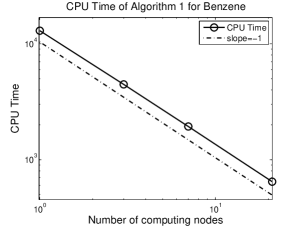
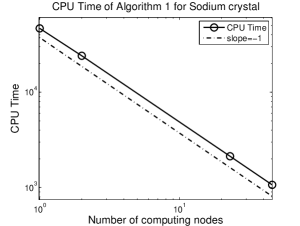
In order to show the scalability of Algorithm 1, we first present the numerical results for Benzene and Sodium crystal. We test the parallel scalability for Benzene and Sodium crystal when different numbers of computing nodes are used. The desired eigenpairs are distributed to different computing nodes and each computing node has the same number of eigepairs to be solved. The number of computing nodes for Benzene and Sodium crystal are set to be and , respectively. The total computational time of Algorithm 1 by using different number of computing nodes are presented in Figure 1. From Figure 1, we can find that Algorithm 1 has a good scalability.
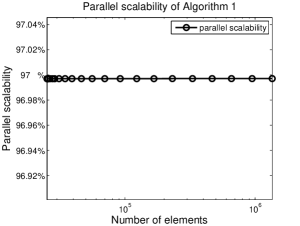
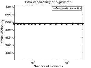
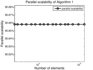
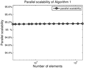
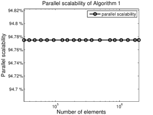
Besides, we also test the parallel efficiency of Algorithm 1 when the mesh size changed while the number of computing nodes remain unchanged. The parallel efficiency is calculated through the formula , where denote the serial computing time, denotes the parallel computing time and denotes the number of computing nodes. The numbers of computing nodes are chosen as that of the required eigenpairs for the five models, i.e. , respectively. We demonstrate the trend of parallel efficiency according to the refinement of mesh and the corresponding results are presented in Figures 2-3. From Figures 2-3, we can also find that Algorithm 1 has a good scalability in different adaptive spaces.
4.3 Numerical performance of Algorithm 1
In this subsection, we show the numerical performances for the five Kohn-Sham models. We first test the orthogonality of the approximate eigenfunctions derived from Algorithm 1. Tables 9-13 present the biggest values of inner products of the eigenfunctions corresponding to the different eigenvalues in each level of the adaptive finite element spaces for the five Kohn-Sham models. The results presented in Tables 9-13 show that Algorithm 1 can keep the orthogonality of the eigenfunctions along with the refinement of mesh.
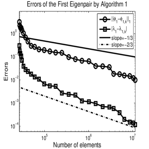
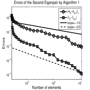
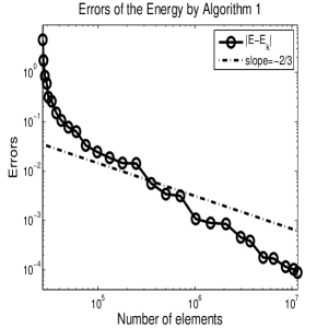
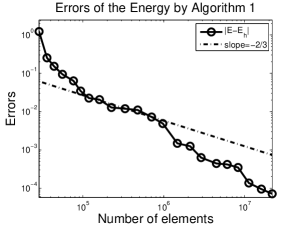
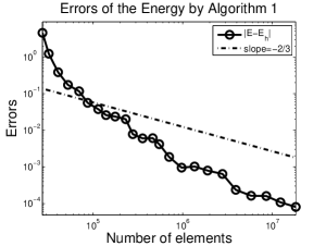
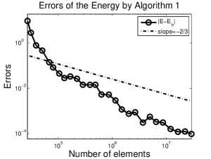
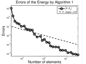
Next, we investigate the error estimates of the approximate solutions derived by Algorithm 1 for the five models.
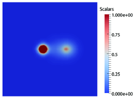
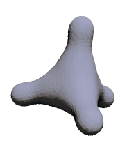
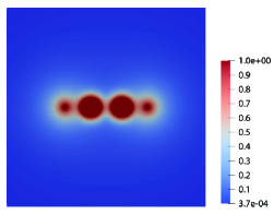
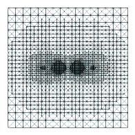
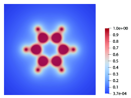
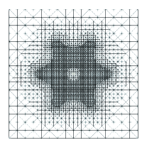
Figures 4, 6, 7, 8 and 9 gives the graphic exhibition of the numerical results by Algorithm 1. The corresponding results associated with error estimates are presented in Figures 5, 6, 7, 8 and 9, which show that Algorithm 1 is capable of deriving the optimal error estimates.
| Mesh Level | 1 | 2 | 3 | 4 | 5 |
|---|---|---|---|---|---|
| Inner Product | 0.0000e-0 | 1.9498e-5 | 1.0040e-5 | 6.1033e-6 | 1.4316e-5 |
| Mesh Level | 6 | 7 | 8 | 9 | 10 |
|---|---|---|---|---|---|
| Inner Product | 3.2717e-6 | 2.8455e-6 | 8.3587e-7 | 1.9357e-6 | 6.5374e-7 |
| Mesh Level | 11 | 12 | 13 | 14 | 15 |
|---|---|---|---|---|---|
| Inner Product | 1.7357e-6 | 4.7698e-7 | 3.1525e-7 | 2.2424e-7 | 2.8045e-7 |
| Mesh Level | 16 | 17 | 18 | 19 | 20 |
|---|---|---|---|---|---|
| Inner Product | 8.8124e-7 | 1.2938e-7 | 5.5421e-8 | 2.5063e-7 | 4.8012e-8 |
| Mesh Level | 21 | 22 | 23 | 24 | 25 |
|---|---|---|---|---|---|
| Inner Product | 3.7354e-8 | 2.4355e-8 | 8.3322e-9 | 2.1567e-8 | 5.3984e-9 |
| Mesh Level | 1 | 2 | 3 | 4 | 5 |
|---|---|---|---|---|---|
| Inner Product | 0.0000e-0 | 3.5339e-5 | 2.6196e-5 | 7.8513e-6 | 2.1434e-5 |
| Mesh Level | 6 | 7 | 8 | 9 | 10 |
|---|---|---|---|---|---|
| Inner Product | 5.4062e-6 | 1.6346e-5 | 4.6419e-6 | 2.7387e-6 | 2.6765e-6 |
| Mesh Level | 11 | 12 | 13 | 14 | 15 |
|---|---|---|---|---|---|
| Inner Product | 1.2886e-6 | 1.1922e-6 | 8.6543e-7 | 1.5147e-6 | 7.7643e-7 |
| Mesh Level | 16 | 17 | 18 | 19 | 20 |
|---|---|---|---|---|---|
| Inner Product | 6.2544e-7 | 3.3645e-7 | 1.9469e-7 | 2.4036e-7 | 1.0117e-7 |
| Mesh Level | 21 | 22 | 23 | 24 | 25 |
|---|---|---|---|---|---|
| Inner Product | 8.8124e-8 | 1.8111e-7 | 2.5065e-8 | 5.0711e-8 | 1.1934e-8 |
| Mesh Level | 1 | 2 | 3 | 4 | 5 |
|---|---|---|---|---|---|
| Inner Product | 0.0000e-0 | 7.4681e-5 | 6.1964e-5 | 4.0481e-5 | 2.1546e-5 |
| Mesh Level | 6 | 7 | 8 | 9 | 10 |
|---|---|---|---|---|---|
| Inner Product | 5.4252e-6 | 1.4153e-5 | 3.5523e-6 | 1.0320e-5 | 4.1546e-6 |
| Mesh Level | 11 | 12 | 13 | 14 | 15 |
|---|---|---|---|---|---|
| Inner Product | 3.0646e-6 | 2.5461e-6 | 9.4651e-7 | 1.0313e-6 | 1.4862e-6 |
| Mesh Level | 16 | 17 | 18 | 19 | 20 |
|---|---|---|---|---|---|
| Inner Product | 8.6463e-7 | 6.5663e-7 | 7.6741e-7 | 7.2418e-7 | 5.1564e-7 |
| Mesh Level | 21 | 22 | 23 | 24 | 25 |
|---|---|---|---|---|---|
| Inner Product | 8.5362e-8 | 5.2283e-8 | 2.1813e-7 | 4.7199e-8 | 2.5502e-8 |
| Mesh Level | 1 | 2 | 3 | 4 | 5 |
|---|---|---|---|---|---|
| Inner Product | 0.0000e-0 | 3.3343e-4 | 1.6784e-5 | 8.3429e-4 | 7.7229e-5 |
| Mesh Level | 6 | 7 | 8 | 9 | 10 |
|---|---|---|---|---|---|
| Inner Product | 5.5827e-5 | 2.4008e-5 | 2.7386e-5 | 1.4684e-5 | 8.1615e-6 |
| Mesh Level | 11 | 12 | 13 | 14 | 15 |
|---|---|---|---|---|---|
| Inner Product | 1.6854e-5 | 5.3768e-6 | 3.6524e-6 | 3.7026e-6 | 2.5145e-6 |
| Mesh Level | 16 | 17 | 18 | 19 | 20 |
|---|---|---|---|---|---|
| Inner Product | 2.4746e-6 | 1.9326e-6 | 8.4358e-7 | 1.1354e-6 | 7.1456e-7 |
| Mesh Level | 21 | 22 | 23 | 24 | 25 |
|---|---|---|---|---|---|
| Inner Product | 1.1254e-6 | 4.6510e-7 | 5.9616e-7 | 2.1382e-7 | 1.4798e-7 |
| Mesh Level | 26 | 27 | 28 | 29 | 30 |
|---|---|---|---|---|---|
| Inner Product | 7.1642e-8 | 1.3617e-7 | 8.4178e-8 | 7.5464e-8 | 6.3578e-8 |
| Mesh Level | 1 | 2 | 3 | 4 | 5 |
|---|---|---|---|---|---|
| Inner Product | 0.0000e-0 | 8.4713e-4 | 8.0158e-4 | 6.0454e-4 | 4.1687e-4 |
| Mesh Level | 6 | 7 | 8 | 9 | 10 |
|---|---|---|---|---|---|
| Inner Product | 8.5423e-5 | 2.3185e-4 | 6.3291e-5 | 4.8652e-5 | 3.5614e-5 |
| Mesh Level | 11 | 12 | 13 | 14 | 15 |
|---|---|---|---|---|---|
| Inner Product | 4.3523e-5 | 2.5875e-5 | 1.7135e-5 | 8.9253e-6 | 7.9633e-6 |
| Mesh Level | 16 | 17 | 18 | 19 | 20 |
|---|---|---|---|---|---|
| Inner Product | 1.5853e-5 | 1.1443e-5 | 5.6537e-6 | 3.2123e-6 | 3.7452e-6 |
| Mesh Level | 21 | 22 | 23 | 24 | 25 |
|---|---|---|---|---|---|
| Inner Product | 2.2873e-6 | 1.1564e-6 | 7.5720e-7 | 1.4354e-6 | 6.5264e-7 |
| Mesh Level | 26 | 27 | 28 | 29 | 30 |
|---|---|---|---|---|---|
| Inner Product | 5.1215e-7 | 3.8238e-7 | 3.9654e-7 | 2.1426e-7 | 1.0964e-7 |
Finally, in order to show the efficiency of Algorithm 1 more clearly, we compare its computational time with that of the standard AFEM and the standard multilevel correction adaptive method developed in [18]. In our test, we set the same accuracy of energy for all the adopted algorithms. The CPU time (in seconds) is provided in Tables 14 and 15. From Tables 14 and 15, we can find that Algorithm 1 and the standard multilevel correction adaptive algorithm all have better efficiency over the standard AFEM. The saving of the computing time comes from that solving large-scale nonlinear eigenvalue problems is avoided in this two algorithms. Besides, we also can find that Algorithm 1 has a large advantage over the standard multilevel correction adaptive algorithm based on the new computing strategy developed in this paper.
Furthermore, comparing the CPU time of different models presented in Tables 14 and 15, we can find the advantage of Algorithm 1 is more obvious for more complicated models. This is because a more complicated model needs more SCF iteration numbers and this will takes a significant amount of time for the classical methods; while for Algorithm 1, this can be solved efficiently by using the separately handling method for the nonlinear terms and the efficient implementing schemes for the inner iterations. In addition, comparing Tables 14 and 15, we can find the advantage of Algorithm 1 becomes more obvious when the accuracy of energy improves. This is because the computing time for solving the small-scale nonlinear eigenvalue problem (31) is gradually negligible along with the refinement of mesh.
| Time of standard AFEM |
|
Time of Algorithm 1 | |||
|---|---|---|---|---|---|
| Hydrogen-Lithium | 188.93 | 95.74 | 94.67 | ||
| Methane | 738.85 | 321.13 | 272.31 | ||
| Acetylene | 3426.61 | 685.23 | 284.78 | ||
| Benzene | 7311.49 | 1354.75 | 646.16 | ||
| Sodium crystal | 17351.72 | 2629.95 | 1069.04 |
| Time of standard AFEM |
|
Time of Algorithm 1 | |||
|---|---|---|---|---|---|
| Hydrogen-Lithium | 2986.38 | 605.29 | 508.39 | ||
| Methane | 16052.52 | 2494.06 | 1648.14 | ||
| Acetylene | 28091.26 | 3942.35 | 1736.56 | ||
| Benzene | 142339.41 | 12374.82 | 3821.42 | ||
| Sodium crystal | - | 26037.58 | 6562.57 |
5 Conclusion
In this paper, we propose an accelerating multilevel correction adaptive finite element method for the Kohn-Sham equation. The new algorithm benefits from two acceleration strategies. The first one is to separately handle the nonlinear Hartree potential and exchange-correlation potential, which can be solved efficiently by outer iteration and inner iteration. respectively. The second one is to parallelize the algorithm in an eigenpairwise approach. Compared with previous results, a significant improvement of numerical efficiency can be observed from plenty of numerical experiments, which make the new method more suitable for the practical problems.
References
- [1] R. A. Adams, Sobolev spaces, Academic Press, New York, 1975.
- [2] I. Babuška and T. Strouboulis, The finite element method and its reliability, Numerical Mathematics and Scientific Computation, The Clarendon Press, Oxford University Press, New York, 2001.
- [3] G. Bao, G. Hu and D. Liu, An -adaptive finite element solver for the calculation of the electronic structures, J. Comput. Phys., 231 (2012), 4967–4979.
- [4] G. Bao, G. Hu and D. Liu, Numerical solution of the Kohn-Sham equation by finite element methods with an adaptive mesh redistribution technique, J. Sci. Comput., 55(2) (2012), 372–391.
- [5] T. L. Beck, Real-space mesh techniques in density functional theory, Rev. Modern Phys., 72 (2000), 1041–1080.
- [6] D. Bowler, R. Choudhury, M. Gillan and T. Miyazaki, Recent progress with large scale ab initio calculations: The CONQUEST code, Phys. Status Solidi B, 243 (2006), 989–1000.
- [7] E. J. Bylaska, M. Host and J. H. Weare, Adaptive finite element method for solving the exact Kohn-Sham equation of density functional theory, J. Chem. Theory Comput., 5 (2009), 937–948.
- [8] E. Cancès, R. Chakir and Y. Maday, Numerical analysis of the planewave discretization of some orbital-free and Kohn-Sham models, ESAIM Math. Model. Numer. Anal., 46 (2012), 341–388.
- [9] A. Castro, H. Appel, M. Oliveira, C. A. Rozzi, X. Andrade, F. Lorenzen, M. A. L. Marques, E. K. U. Gross, A. Rubio, Octopus: A tool for the application of time-dependent density functional theory, Phys. Status Solidi B, 243 (2006), 24650–2488.
- [10] J. R. Chelikowsky, N. Troullier and Y. Saad, Finite-difference pseudopotential method: Electronic structure calculations without a basis, Phys. Rev. Lett., 72 (1994), 1240–1243.
- [11] H. Chen, X. Gong, L. He, Z. Yang and A. Zhou, Numerical analysis of finite dimensional approximations of Kohn-Sham models, Adv. Comput. Math., 38 (2013), 225–256.
- [12] H. Chen, H. Xie and F. Xu, A full multigrid method for eigenvalue problems, J. Comput. Phys. 322 (2016), 747-759.
- [13] W. Dörfler, A convergent adaptive algorithm for Poisson’s equation, SIAM J. Numer. Anal., 33(3) (1996), 1106–1124.
- [14] J. Fang, X. Gao and A. Zhou, A Kohn-Sham equation solver based on hexahedral finite elements, J. Comput. Phys., 231 (2012), 3166–3180.
- [15] L. Genovese, B. Videau, M. Ospici, T. Deutsch, S. Godecker, J. F. Mèhaut, Daubechies wavelets for high performance electronic structure calculations: The BigDFT project, C. R. Mécanique, 339 (2011), 149–164.
- [16] W. J. Hehre, R. F. Stewart and J. A. Pople, Self-consistent molecular-orbital methods. I. Use of Gaussian expansions of Slater-type atomic orbitals, J. Chem. Phys., 51 (1969), 2657–2664.
- [17] B. Hermannson and D. Yevick, Finite-element approach to band-structure analysis, Phys. Rev. B, 33 (1986), 7241–7242.
- [18] G. Hu, H. Xie, F. Xu, A multilevel correction adaptive finite element method for Kohn-Sham equation, J. Comput. Phys., 355 (2018), 436–449.
- [19] F. Jensen, Introduction to Computational Chemistry, Wiley Publishers, 1999.
- [20] S. Jia, H. Xie, M. Xie and F. Xu, A full multigrid method for nonlinear eigenvalue problems, Science China: Mathematics, 59 (2016), 2037–2048.
- [21] S. Kotochigova, Z.H. Levine, E.L. Shirley, M.D. Stiles, and C.W. Clark, Local-density-functional calculations of the energy of atoms, Phys. Rev. A., 55(1997), 191–199.
- [22] R.B. Lehoucq, D.C. Sorensen and C. Yang, ARPACK Users’ Guide, Solution of large-scale eigenvalue problems with implicitly restarted Arnoldi methods, (SIAM, Philadelphia, PA, 1998).
- [23] L. Lehtovaara, V. Havu and M. Puska, All-electron density functional theory and time-dependent density functional theory with high-order finite elements, J. Chem. Phys., 131 (2009), 054103.
- [24] L. Lin, J. Lu, L. Ying and W. E, Adaptive local basis set for Kohn-Sham density functional theory in a discontinuous Galerkin framework I: Total energy calculation, J. Comput. Phys., 231 (2012), 2140–2154.
- [25] Q. Lin and H. Xie, A multi-level correction scheme for eigenvalue problems, Math. Comp., 84(291) (2015), 71–88.
- [26] Q. Lin, H. Xie and J. Xu, Lower bounds of the discretization for piecewise polynomials, Math. Comp., 83 (2014), 1–13.
- [27] A. Masud and R. Kannan, B-splines and NURBS based finite element methods for Kohn-Sham equations, Comput. Methods Appl. Mech. Engrg., 241-244 (2012), 112–127.
- [28] N. A. Modine, G. Zumbach and E. Kaxiras, Adaptive-coordinate real-space electronic-structure calculations for atoms, molecules and solids, Phys. Rev. B, 55 (1997), 289–301.
- [29] H. Nishioka, K. Hansen and B. R. Mottelson, Supershells in metal clusters, Phys. Rev. B, 42(15) (1990), 9378–9386.
- [30] J. E. Pask, B. M. Klein, C. Y. Fong and P. A. Sterne, Real-space local polynomial basis for solid-state electronic-structure calculations: A finite element approach, Phys. Rev. B, 59 (1999), 12352–12358.
- [31] J. E. Pask, B. M. Klein, P. A. Sterne and C. Y. Fong, Finite element methods in electronic-structure theory, Comput. Phys. Comm., 135 (2001), 1–34.
- [32] J. E. Pask and P. A. Sterne, Finite element methods in ab initio electronic structure calculations, Model. Simul. Mater. Sci. Eng., 13 (2005), R71–R96.
- [33] J. P. Perdew and A. Zunger, Self-interaction correction to density-functional approximations for many-electron systems, Phys. Rev. B, 23 (1981), 5048–5079.
- [34] V. Schauer and C. Linder, All-electron Kohn-Sham density functional theory on hierarchic finite element spaces, J. Comput. Phys., 250 (2013), 644–664.
- [35] C.K. Skylaris, P. D. Haynes, A. A. Mostofi and M. C. Payne, Introducing ONETEP: Linear-scaling density functional simulations on parallel computers, J. Chem. Phys., 122 (2005), 084119.
- [36] J. M. Soler, E. Artacho, J. D. Gale, A. García, J. Junquera, P. Ordejn and D.Sañchez-Portal, The siesta method for ab initio order-n materials simulation, J. Phys. Condens. Matter, 14 (2002), 2745–2779.
- [37] P. Suryanarayana, V. Gavini, T. Blesgen, K. Bhattacharya and M. Ortiz, Non-periodic finite-element formulation of Kohn-Sham density functional theory, J. Mech. Phys. Solids, 58 (2010), 256–280.
- [38] E. Tsuchida and M. Tsukada, Electronic-structure calculations based on the finite-element method, Phys. Rev. B, 52 (1995), 5573–5578.
- [39] E. Tsuchida and M. Tsukada, Adaptive finite-element method for electronic structure calculations, Phys. Rev. B, 54 (1996), 7602–7605.
- [40] E. Tsuchida and M. Tsukada, Large-scale electronic-structure calculations based on the adaptive finite element method, J. Phys. Soc. Jpn., 67 (1998), 3844–3858.
- [41] S. R. White, J. W. Wilkins and M. P. Teter, Finite element method for electronic structure, Phys. Rev. B, 39 (1989), 5819–5830.
- [42] J. M. Wills and B.R. Cooper, Synthesis of band and model Hamiltonian theory for hybridizing cerium systems, Phys. Rev. B, 36 (1987), 3809–3823.
- [43] H. Xie, A multigrid method for eigenvalue problem, J. Comput. Phys., 274 (2014), 550–561.
- [44] H. Xie, A multigrid method for nonlinear eigenvalue problems, Science China: Mathematics (Chinese), 45(8) (2015), 1193–1204.
- [45] H. Xie and M. Xie, A multigrid method for ground state solution of Bose-Einstein condensates, Communications in Computational Physics, 19 (2016), 648–662.
- [46] F. Xu, H. Xie and N. Zhang, A parallel augmented subspace method for eigenvalue problems, SIAM J. Sci. Comput., 42(5) (2020), A2655–A2677.
- [47] D. Zhang, L. Shen, A. Zhou and X. Gong, Finite element method for solving Kohn-Sham equations based on self-adaptive tetrahedral mesh, Phys. Lett. A, 372 (2008), 5071–5076.
- [48] N. Zhang, F. Xu and H. Xie, An efficient multigrid method for ground state solution of Bose-Einstein condensates, Int. J. Numer. Anal. Model., 2019, 16(5), 789–803.