Pressureless stationary solutions in a Newton-Yukawa gravity model

Abstract

Non-minimally coupled curvature-matter gravity models are an interesting alternative to the Theory of General Relativity and to address the dark energy and dark matter cosmological problems. These models have complex field equations that prevent a full analytical study. Nonetheless, in a particular limit, the behavior of a matter distribution can, in these models, be described by a Schrödinger-Newton system. In nonlinear optics, the Schrödinger-Newton system can be used to tackle a wide variety of relevant situations and several numerical tools have been developed for this purpose. Interestingly, these methods can be adapted to study General Relativity problems as well as its extensions. In this work, we report the use of these numerical tools to study a particular non-minimal coupling model that introduces two new potentials, an attractive Yukawa potential and a repulsive potential proportional to the energy density. Using the imaginary-time propagation method we have shown that stationary solutions arise even at low energy density regimes.

I Introduction

In recent years various alternative theories of gravity have been proposed to extend General Relativity (GR) and studied to address some well-known cosmological difficulties such as dark energy and dark matter. Non-minimally coupled (NMC) curvature-matter gravity models Bertolami et al. (2007) were proposed to approach these problems under a different perspective, but are also particularly interesting as they give rise to a rich lore of features and have a wide range of astrophysical and cosmological implications (see, for instance, Ref. Bertolami and Páramos (2014), for a review). NMC curvature-matter gravity models extend GR and the so-called $f(R)$ models of gravity by allowing for an extra curvature coupling to the matter Lagrangian density. In its most general setting, NMC curvature-matter gravity models are characterized by two functions of the scalar curvature, $f_{1,2}(R)$. Function $f_{1}(R)$ allows for going beyond the linear scalar curvature term of the Einstein-Hilbert action whereas $f_{2}(R)$ generalizes the minimal coupling between matter and geometry that involves the square root of the positive valued determinant of the metric, $\sqrt{|g|}$, so to keep the element of volume invariant, and covariant derivatives. The non-minimal coupling gives rise to very convoluted field equations that cannot, in general, be treated analytically and poses challenges to the existing numerical methods. However, as previously shown Ferreira et al. (2020), under the right assumptions, the field equations for specific matter distributions can be transformed into a Schrödinger-Newton system of equations.

The Schrödinger-Newton model, also known in the literature as Schrödinger-Poisson, is commonly used in nonlinear optics for describing light propagating in nonlinear and nonlocal media, under the paraxial approximation Quiroga-Teixeiro and Michinel (1997); Alberucci et al. (2014); Roger et al. (2016); Michel et al. (2018), and self-gravitating Bose-Einstein condensates Chavanis and Delfini (2011), among other situations Bahrami et al. (2014); Pethick and Smith (2008); Carusotto and Ciuti (2013). Due to the wide applicability of this model, many numerical schemes were developed Taha and Ablowitz (1984), with the Split-Step Fourier method (SSFM) being the most suitable one. This numerical scheme, apart from being easy to implement, also allows searching for the existence of stationary solutions through the imaginary-time propagation method Chiofalo et al. (2000); Lehtovaara et al. (2007), whereby propagating an initial random ansatz the system ultimately converges into a stationary solution, if it exists. When both these schemes are applied to these new theories of gravity, they open the possibility to study the dynamics imposed by the model settings and search for the existence of new stationary configurations simply and efficiently. Thus, this set of techniques stand as a promising tool to probe these new gravity models, as they can be used to quickly test and impose constraints on the model features. This idea was previously explored by our research group for NMC models Ferreira et al. (2020), however in this work we focus on a different approximation regime and consider the imaginary-time propagation method to search for stationary solutions.

Besides the computational advantages, the Schrödinger-Newton approach is also promising as it can be used to develop table-top experiments that, under certain conditions, can emulate the dynamical features of some cosmological systems. These phenomena range from gravitational effects Bekenstein et al. (2015), boson stars Roger et al. (2016), scalar dark-matter models Navarrete et al. (2017); Paredes et al. (2020), false-vacuum decay Fialko et al. (2015); Braden et al. (2019), to acoustic black-holes Faccio et al. (2012); Marino (2008); Vocke et al. (2018) to study the formation of Hawking-radiation Drori et al. (2019); de Nova et al. (2019), superradiance Braidotti et al. (2020); Prain et al. (2019), the Penrose effect Solnyshkov et al. (2019) and even the formation of scalar clouds Ciszak and Marino (2021). At the conceptual level, these so-called optical analogue experiments allow to test features of the theoretical models in an experimental setting, gaining new insights through interdisciplinary research. Leveraging this cross-fertilization, the alternative theories of gravity explored in this work stand as an interesting candidate for further development and implementation of a new class of analogues dedicated to explore their dynamics under controlled experimental conditions.

In this work, we make use of advanced high-performance computing tools previously developed at our research group in the context of nonlinear optics Ferreira et al. (2018, 2019); Silva et al. (2017), to detect and to explore how NMC curvature-matter models of gravity give rise to stationary large scale distributions of mass. In particular, we focus on a particular non-minimal coupled curvature-matter gravity model, where functions $f_{1}(R)$ and $f_{2}(R)$ are expanded up to the second and first order in the curvature $R$, respectively, and assume that matter at the relevant scales behaves as a fluid. These assumptions allow for describing the system by a set of hydrodynamic equations, and two potentials arise in this context, an attractive Yukawa potential besides the Newtonian one, and a repulsive potential proportional to the energy density. Following this procedure, the Schrödinger-Newton model is obtained through the application of a Madelung transformation Madelung (1927), and, by considering the Thomas-Fermi approximation, we show that this gravity model supports stationary solutions in the absence of a pressure term. We then calculate these solutions through the imaginary-time propagation method and compare the results with some analytical predictions. Finally, we discuss the implications of these pressureless solutions in the context of these alternative gravity models.

II Gravitational Model

In this work we will focus on a previously proposed NMC curvature-matter gravity model Bertolami et al. (2007) that admits two functions of the scalar curvature, $f_{1}(R)$, and, $f_{2}(R)$. The physical model is then described by the following action:

$$S=\int\mathrm{d}^{4}x\sqrt{|g|}\left[\frac{1}{2}f_{1}(R)+\left(1+f_{2}(R)\right)\mathcal{L}_{m}\right]\,,$$ (1)

where $\mathcal{L}_{m}$ is the matter Lagrangian density, with GR trivially recovered for the choice:

$$f_{1}(R)=\frac{R}{\kappa}\,,\quad f_{2}(R)=0\,.$$ (2)

In the metric formalism, the field equations for this model are:

$$\begin{split}\left(F_{1}+2F_{2}\mathcal{L}_{m}\right)&R_{\mu\nu}-\frac{f_{1}}{2}g_{\mu\nu}=\left(1+f_{2}\right)T_{\mu\nu}\\ &+\left(\nabla_{\mu}\nabla_{\nu}-g_{\mu\nu}\square\right)\left(F_{1}+2F_{2}\mathcal{L}_{m}\right)\,,\end{split}$$ (3)

where $F_{i}\equiv\partial f_{i}/\partial R$, and $\Box$ is the D’Alembertian operator defined as $\Box=g^{\mu\nu}\nabla_{\mu}\nabla_{\nu}$ in terms of covariant derivatives from a Levi-Civita connection.

From these equations it is possible to deduce one of the most distinctive features of the NMC curvature-matter gravity, namely that the energy-momentum tensor is not covariantly conserved. In fact, taking the covariant derivative of Eq. (3) we get:

$$\nabla_{\mu}T^{\mu\nu}=\frac{F_{2}}{1+f_{2}}\left(g^{\mu\nu}\mathcal{L}_{m}-T^{\mu\nu}\right)\nabla_{\mu}R\,.$$ (4)

Additional implications of the model have been extensively discussed in the literature and can be found in previously works of one of the authors Bertolami and Páramos (2014); Bertolami et al. (2008); Bertolami and Gomes (2014, 2017); Bertolami et al. (2018); Bertolami and Páramos (2020); Bertolami and Gomes (2020). Considering the functions $f_{i}(R),\,i=1,2$ to be analytical around $R=0$, we can make use of a Taylor expansion and express

$$\begin{split}f_{1}(R)&=\frac{1}{\kappa}(a_{1}R+a_{2}R^{2})+\mathcal{O}(R^{3})\,,\\ f_{2}(R)&=q_{1}R+\mathcal{O}(R^{2})\,.\end{split}$$ (5)

This expansion have been examined in the context of oceanic experiments March et al. (2019) and consistency with the well known Cassini experiment is currently under scrutiny March et al. (2021). Here, we will extend beyond these scales and explore it at an astrophysical context.

Taking the nonrelativistic limit, the solution of the field equations gives for the $00$ component of the metric March et al. (2017)

$$g_{00}=-1+\frac{2}{c^{2}}\left[U+\frac{1}{3}\left(1-\frac{q_{1}}{a_{2}}\right)Y\right]+\mathcal{O}(c^{-4})\,$$ (6)

containing both a Newtonian and a Yukawa potentials, defined through the equations

$$\nabla^{2}U=-4\pi G\rho,$$ (7)

$$\left(\nabla^{2}-\frac{1}{\lambda^{2}}\right)Y=-4\pi G\rho\,,$$ (8)

respectively. In this regime, the resulting hydrodynamic equations for a fluid with energy density, $\rho$, isotropic pressure, $P$, and velocity, $\vec{v}$, are March et al. (2019)

$$\frac{\partial\rho}{\partial t}+\nabla(\rho\vec{v})=0$$ (9)

$$\frac{\partial\vec{v}}{\partial t}+(\vec{v}\cdot\nabla)\vec{v}=\nabla\left[U+\alpha_{0}Y-V_{p}-\frac{4\pi}{3}G\lambda^{2}\theta^{2}\rho\right],$$ (10)

where $\theta=q_{1}/a_{2}$, $\alpha_{0}=(1-\theta)^{2}/3$ and $\lambda=\sqrt{6a_{2}}$. For the pressure potential, $V_{p}$, we will assume a polytropic relation between $\rho$ and $P$ given by $P=w\rho^{n}$, with $w$ and $n$ being constants chosen for each physical situation, which gives

$$V_{p}=\begin{cases}w\ln(\rho)&n=1\\ \frac{nw}{n-1}\rho^{n-1}&n>1\lor n<0\end{cases}\,.$$ (11)

Comparing Eq. (10) with the ones obtained from the Newtonian limit of GR it is clear that two additional terms appear: the Yukawa potential, and a term depending on the energy density, with a proportionality coefficient $4\pi G\lambda^{2}\theta^{2}/3$. In the subsequent sections we will explore some of the consequences of these terms.

Before advancing we point out that an additional assumption $a_{2}>0$ is required so that the range of the Yukawa potential is real and this is related to the Dolgov-Kawasaki stability criterion Bertolami and Sequeira (2009); Nojiri and Odintsov (2003):

$$f_{1}^{\prime\prime}(R)+2\mathcal{L}_{m}f_{2}^{\prime\prime}(R)\geq 0\,.$$ (12)

This requirement stems from the fact that the field equations for NMC curvature-matter gravity are greater than second order. Thus, the Ricci scalar is not algebraically related to the trace of the energy-momentum tensor but rather given by a differential equation. This means that $R$ is, in fact, a dynamical field and the Dolgov-Kawasaki stability criterion corresponds to the requirement that the field effective mass ($1/\lambda)$ is positive.

III A cosmology-like setting

Describing the gravitational system as a fluid characterized by the set of hydrodynamic Eqs. (9) and (10), is quite useful to explore the dynamics of the model as, by performing a Madelung transformation Madelung (1927), the set of equations are transformed into a Schrödinger-Newton-Yukawa model Johnston et al. (2010). This transformation is achieved by writing $\psi=\sqrt{\rho}e^{i\Phi/\nu}$, where $\nu$ is an adjustable parameter with the same dimensions as the velocity field $\Phi$, such that $\rho=|\psi|^{2}$ and $\vec{v}=\nabla\Phi$ are the density and velocity of the fluid, respectively. By substituting this into the hydrodynamic equations, re-scaling the field $\psi=\frac{\psi}{\sqrt{\rho_{0}}}$ and normalizing the equations, it is straightforward to show that

$$\begin{split}i\frac{\partial\psi}{\partial t}=-\frac{1}{2}\nabla^{2}\psi-\left[U+\alpha_{0}Y-\frac{\theta^{2}\Gamma^{2}}{3}|\psi|^{2}\right]\psi\\ +\gamma_{0}\frac{n}{n-1}|\psi|^{2(n-1)}\psi+V_{B}\psi\end{split}$$ (13)

where

$$\nabla^{2}U =-|\psi|^{2},$$ (14)

$$\left(\nabla^{2}-\frac{1}{\Gamma^{2}}\right)Y =-|\psi|^{2},$$ (15)

$\Gamma$ is the normalized $\lambda$ parameter, and $\gamma_{0}=\omega\rho_{0}^{n-3/2}/(\nu\sqrt{4\pi G})$ is a constant that depends on the polytropic exponent $n$ and measures the strength of the pressure term. The last term in the Schrödinger equation is the well known Bohm quantum potential or quantum pressure, $V_{B}=\nabla^{2}\sqrt{\rho}/(2\sqrt{\rho})$. This potential can be removed from equation (13), but it shows up instead in the hydrodynamic equations like a pressure gradient. This potential has no equivalent in classical fluids, and it is usually found when attempting to describe quantum mechanics from a hydrodynamic perspective or in nonlinear optics due to the diffraction. In the present context we can estimate the effect of this potential by considering $\rho$ to be given by a Gaussian distribution with width $R$, and it is the straightforward to show that $V_{B}\sim 1/R^{2}$. Thus, the Bohm potential is only important in circumstances where the energy density $\rho$ varies greatly over the scale of interest ($\sim 1$), that is in collapse situations. However, these scenarios will not be considered in this work, and thus the Bohm potential can be safely disregarded. Finally, it is pertinent to point out that, despite the use of some quantum mechanics features, it is not our aim to describe our model from a quantum perspective, but rather use the mathematical procedure provided by the Madelung transformation Madelung (1927), which allows transforming the complete Vlasov-Poisson system into a system of equations that are easier to work with.

Before advancing we note that equations (13), (14) and (15) admit, in specific contexts, self similar solutions, described by the following scaling transformation

$$\vec{r}\rightarrow\vec{r}^{\prime} =\lambda_{S}^{-1}\vec{r}$$ (16)

$$t\rightarrow t^{\prime} =\lambda_{S}^{-2}t$$ (17)

$$\psi\left(\vec{r},t\right)\rightarrow\psi^{\prime}\left(\vec{r}^{\prime},t^{\prime}\right) =\lambda_{S}^{2}\psi\left(\lambda_{S}\vec{r}^{\prime},\lambda_{S}^{2}t^{\prime}\right),$$ (18)

with $\Gamma^{\prime}=\lambda_{S}^{-1}\Gamma$. Indeed, it is easy to show that these relations are valid when the pressure term is negligible or when the polytropic exponent $n=3/2$. Thus, the solutions found under these assumptions are not restricted to the original setting of the system, but can be transformed to describe other systems at different spatial scales. Furthermore, this is also important for testing the validity of the gravitational model, since it is possible to search for scaling factors that correctly scale a certain solution that fits some particular observational data. This fact will be explored later when we focus on the pressureless regime.

A Numerical Methods

The SSFM is commonly regarded as one of the most suitable schemes for the study of the Schrödinger-Newton-Yukawa system Taha and Ablowitz (1984), balancing accuracy with performance. It consists in integrating the system of equations in small steps by transforming the field between the reciprocal and direct spaces, as the kinetic term is better integrated in the first space, whereas the nonlinear potentials in the former. Besides yielding accurate results, this implementation allows to takes advantage from parallel computing techniques and exploit high throughput hardware such as Graphical Processing Units(GPU) for performing complex simulations in reasonable spans of time. For more details about the numerical scheme and its implementation see Refs. Ferreira et al. (2019, 2020), and references therein.

The most straightforward use of the method applied to this system is to explore the dynamics of energy distributions governed by the alternative gravity model and to examine the impact of its parameters. However, an interesting feature is that the method can also be used as a tool to search for stationary solutions. The technique for this purpose is known as the Imaginary-time propagation method (ITP) and consists in performing a Wick rotation on the time parameter $t\rightarrow-it$ Chiofalo et al. (2000); Lehtovaara et al. (2007). This transformation converts Eq. (13) into a diffusion-like equation with emission and absorption terms. By propagating an initial random ansatz and ensuring that the total mass is conserved, the system converges to its ground state as $t\rightarrow\infty$, see Figure 1. As convergence criteria we choose the variation in the energy between integration steps to be below a certain threshold, where the energy is calculated from the Hamiltonian of the system

$$\begin{split}\mathcal{H}=\frac{1}{2}|\nabla\psi|^{2}+\frac{\theta^{2}\Gamma^{2}}{6}|\psi|^{4}+\frac{\gamma_{0}}{n-1}|\psi|^{2n}\\ -\frac{1}{2}U|\psi|^{2}-\frac{\alpha_{0}}{2}Y|\psi|^{2}.\end{split}$$ (19)

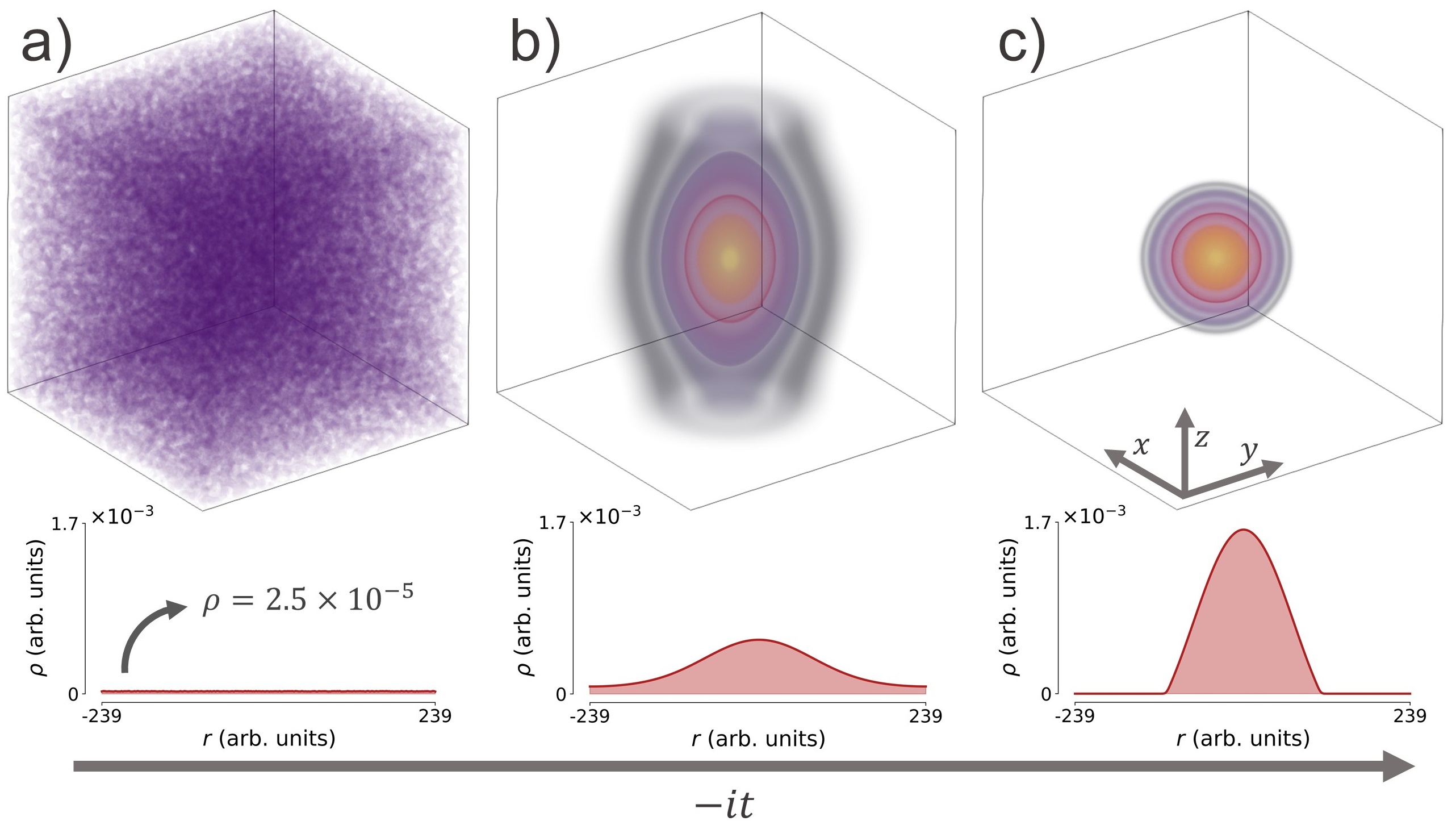
Figure 1: Tree-dimensional representation of the Imaginary-time propagation method for a solution with $\Gamma=60$ and $\alpha_{0}=1\times 10^{-10}$. An initial random ansatz, given by Eq. (27) and corresponding to a), is propagated in an imaginary time scheme, and after some time the initial field converges into a stationary solution. b) The solution after $\sim 119750$ iterations ($t\sim 0.54$ Byr). c) The final solution after $\sim 497500$ iterations ($t\sim 2.18$ Byr). The bottom slices are cuts along the $z$-axis. The solutions are calculated in a tree-dimensional grid with $[256\times 256\times 256]$ points. In this figure and in the following results, in order to convert from the normalized into the physical units, it was considered $\rho_{0}=1\times 10^{-20}kgm^{-3}$ and $\nu=1m^{2}s^{-1}$.

The SSFM complemented with the ITPM is a robust and stable numerical scheme to explore the existence of stationary solutions. Still, depending on the parameters of the system, it can become numerically unstable. In particular, if we neglect the Bohm potential and the pressure term, the most critical term is the term proportional to the energy density, since in order to ensure the stability of the numerical scheme Chiofalo et al. (2000), we have to ensure that

$$\max\left(\left|\frac{\Gamma^{2}\theta^{2}}{3}|\psi|^{2}\Delta t\right|\right)<1,$$ (20)

where $\Delta t$ is the integration step. This imposes limits on the numerical model, since, for large values of $\Gamma$, very small integration steps are required, which, on its turn, can increase the calculations time up to days or even months. On the other hand, we could also decrease the value of the normalized energy density, however, this would require values with limited physical interest. Having this term well controlled, the remaining ones are shown to be stable. Thus, although the numerical scheme does not impose a restrictive limit on the parameters that can be used, we are limited by the available time to compute the solutions and ultimately by the precision of the machine.

IV Stationary Solutions

The existence of stationary solutions requires a balance between the attractive and repulsive potentials which can be easily identified in the gravitational model considered in this work. On one hand, the potentials $U$ and $Y$ correspond to the attractive ones, and in the absence of counteracting forces, they force the system into a collapse. On the other hand, the remaining potentials, namely the pressure and the term proportional to the energy density, will force the system to expand. In general, the repulsion that balances the collapse is maintained by a collaboration between these two potentials. However, for systems where the pressure term can be neglected, it is interesting to notice that the current model may still allow the existence of solutions if solely sustained by the term proportional to the energy density. These stationary solutions, which will be investigated in the subsequent sections, are specific of the model under consideration and found no counterpart in GR nor in previously explored NMC curvature-matter gravity models Ferreira et al. (2020).

A Analytical Approach

To investigate the possibility of such stationary solutions we first explore the systems with an analytical approach, starting by recalling the hydrodynamic equation (10) with the Bohm potential. We assume that we are in an astrophysical scenario where we can neglect the pressure term (pressureless fluid) as well as the Yukawa potential, motivated by the fact that the $\alpha_{0}$ parameter shall be negligible according to known observational bounds Raffai et al. (2011). In a stationary regime, where $\partial_{t}\psi\rightarrow 0$ and $\vec{v}=0$, the hydrodynamic Eq. (10) can be rewritten, in dimensionless units, as

$$\rho+\frac{\theta^{2}\Gamma^{2}}{3}\nabla^{2}\rho-\frac{1}{2}\nabla^{2}\left(\frac{\nabla^{2}\sqrt{\rho}}{\sqrt{\rho}}\right)=0.$$ (21)

Since we are interested in solutions at large scales, the Bohm potential can be safely neglected, a simplification that corresponds to the common Thomas-Fermi (TF) approximation. Alternately, this approximation can be interpreted as if the kinetic term in Schrödinger Eq. (13) could be neglected, since at large scales the contribution from this term to the total energy can be disregarded. Thus, in this approximation we have that

$$\rho+\frac{\theta^{2}\Gamma^{2}}{3}\nabla^{2}\rho=0,$$ (22)

which has an exact solution Chandrasekhar (1939); Chavanis and Delfini (2011) given by

$$\rho(r)=\begin{cases}\frac{\rho_{M}\mathcal{R}}{\pi r}\sin\left(\frac{\pi r}{\mathcal{R}}\right)&r\leq\mathcal{R}\\ 0&r>\mathcal{R}\end{cases}\,,$$ (23)

where the maximum density $\rho_{M}$ can be obtained in terms of the total mass of the system, $M$, by integration of the solution over the volume as

$$\rho_{M}=\frac{\pi M}{4\mathcal{R}^{3}},$$ (24)

and the radius of the solution $\mathcal{R}$ at which the energy density vanishes (compact support) is

$$\mathcal{R}=\frac{\pi\theta\Gamma}{\sqrt{3}}.$$ (25)

It is interesting to notice that this value only depends on the gravitational parameters of the model, $\theta$ and $\Gamma$, and is independent of the total mass of the system. However, we need to be careful since both, too large or too small masses, can violate the assumptions used for the TF approximation. In the first scenario, systems of larger mass are associated with an higher density. In this case, the pressureless regime is no longer valid, breaking the initial assumption of Eq. (22). On the opposite side, the small mass limit is associated with an ultra low-density of the system for which the potential proportional to the energy density can become of the same order of magnitude as the Bohm potential. In such case, which happens when

$$\frac{1}{\mathcal{R}^{2}}\sim\frac{\theta^{2}\Gamma^{2}}{3}\frac{M}{\mathcal{R}^{3}}\Rightarrow M\sim\frac{\pi\sqrt{3}}{\theta\Gamma},$$ (26)

the contributions of both will be of the same order which also invalidates the TF approximation.

B Numerical Results

Let us now numerically examine the stationary solutions discussed in the previous section with the imaginary-time propagation method depicted in Figure 1. To avoid inducing symmetries in the profile of the solution, we started the simulations with a uniform field of amplitude $A$ destabilized by a small random noise $\epsilon(\vec{r})$

$$\psi(\vec{r},t=0)=A+\epsilon(\vec{r}).$$ (27)

This initial state is propagated under the ITP method and the system ultimately converges towards a stationary solution. In Figure 2 a particular solution is shown in a 3D representation, as well as the relevant potentials. It is easily seen that the solution is stabilized solely by the potential proportional to the energy density and the Newtonian potential, since the contribution from the Yukawa potential is negligible. Furthermore, from Figure 2-b), where normalized slices of the potentials are plotted, the Newtonian and the Yukawa potentials are very similar. This happens because we have to consider large values for the $\Gamma$ parameter in order to satisfy the validity of TF approximation and, in this situation, the Yukawa potential resembles a Newtonian one. Thus, the stationary solutions found in the previous section remain valid even for large values of $\alpha_{0}$, and the effect of this extra nonlocal term can be considered in the hydrodynamic equations as $U\rightarrow(1+\alpha_{0})U$, since $\alpha_{0}Y/\Gamma^{2}\sim 0$.

Figure 2: Representation of a stationary solution with $\Gamma=60$ and $\alpha_{0}=1\times 10^{-10}$. a) 3D representation of the stationary solution and the potential’s profiles. The color scales are in arbitrary units. b) Profile comparison of the potentials.

Figure (3) summarizes the features of the stationary solutions obtained with the solver. Figure 3-a) shows the regions forbidden for the value of $\alpha_{0}$ (grey area) that were obtained through several experiments Raffai et al. (2011). In this Figure is also plotted the region of validity of the TF solutions (blueish zone), which indicates that there are a wide variety of systems, with different spatial scales, that can be described by this model. Figure 3-b) shows the comparison between a numerical and the respective analytical solution, for a certain set of parameters. Both solutions are in good agreement, however, it is important to notice that the numerical solution does not assume the TF approximation, and while the exact solution assumes a compact support, the numerical one extends to infinity. This implies that there is a small fraction of the mass that is beyond $r=\mathcal{R}$. This explains some of the differences between the numerical $\rho_{0}$ and the theoretical prediction, which is below $4\%$. This confirms the existence of solutions that are only supported by the term proportional to the energy density (pressureless solutions) predicted in the previous section. Furthermore, it is also shown the agreement of a scaled solution from another one calculated with $\Gamma=30$, as predicted by the scaling laws in Eq. (18). In Figure 3-c) it is shown the effect of the $\alpha_{0}$ value in the solutions. For $\alpha_{0}\lesssim 1\times 10^{-5}$ the solutions barely change, while for large values we see an increase in the peak density while the solutions radius diminishes, since $R\propto 1/(1+\alpha_{0})$ for large values of $\alpha_{0}$. Nevertheless, we see that the numerical solutions continue to agree quite well with the TF solutions. Furthermore, the solutions plotted in 3-a) are valid for a wide range of $\alpha_{0}$ values, and can cover the regions that are consistent with known bounds.

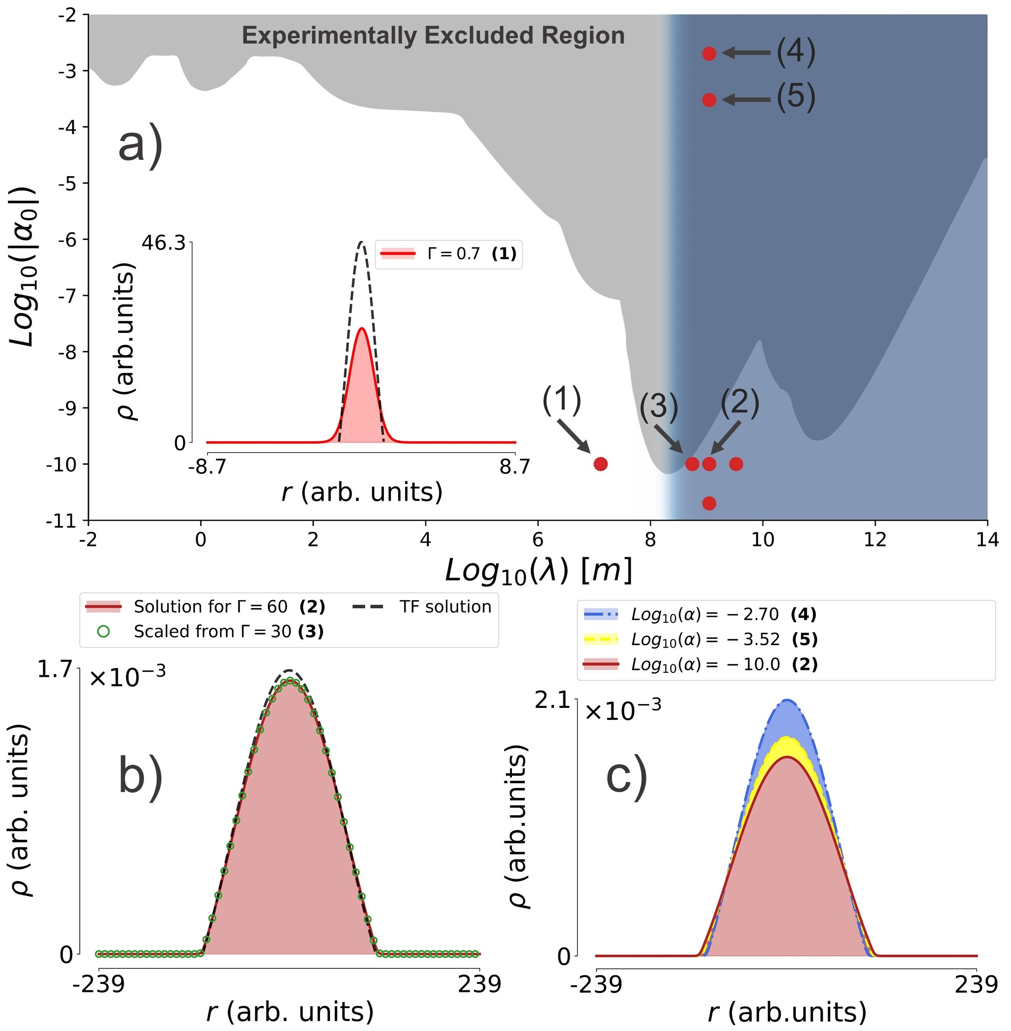
Figure 3: Stationary solutions found by the IMTP. a) Shows the regions prohibited for $\alpha_{0}$ as a function of the parameter $\lambda$, accordingly to Ref. Raffai et al. (2011), and the position of the calculated solutions. The inset shows a solution outside the region of validity of the TF approximation. b) Stationary solution compared with the analytical solution given by Eq. (23) and with a scaled one from a solution with $\Gamma=30$, corresponding to a scaling factor $\lambda_{S}=1/2$. c) Shows the impact of $\alpha_{0}$ on the solution’s profile. The background of a) was adapted from Ref. Raffai et al. (2011).

Finally, the results considered in this work disregard the contribution from the pressure term, but it is now possible to consider more complex situations where this term may be important. In particular, it is relevant to understand the impact of the pressure potential as well as the effect of the polytropic exponent $n$. However, a comprehensive study about the implications of this potential is beyond the scope of the present study, and we leave it for a future work.

V Discussion and Conclusions

In this work we have considered a NMC curvature-matter gravity model described by functions of the scalar curvature, $f_{1}(R)$ and $f_{2}(R)$ given by Eq. (5). Assuming that matter can be described as a fluid, it is found that the system admits a hydrodynamic fluid description Johnston et al. (2010). In this description two additional potentials arise, a Yukawa one and a potential proportional to the energy density. The latter induces a repulsive correction on the fluid equation, and the competition between the attractive potentials and the repulsive ones can, under specific conditions, give origin to stationary solutions. By transforming the hydrodynamic description into the Schrödinger-Newton-Yukawa system, we have confirmed, analytically and then through numerical methods, the existence of this new class of solutions. Furthermore, we also studied the impact of the model parameters in the structure of the solutions and shown that these are compatible with the existing bounds on the parameters of a putative new Yukawa-type interaction.

The numerical recipe used in this work allowed us to circumvent the complexity of the field equation and to obtain a new class of solutions. To our knowledge, the existence of stable solutions without pressure constitutes a new distinct feature of this gravity model that does not exist in GR. The observational implications of this result can be fully appreciated from a more phenomenological perspective in which specific stable and stationary gravity sustainable structures are identified so that their parameters can be matched with the ones of our gravity model. This type of analysis has been previously considered, for instance, in an oceanographic context March et al. (2019) and the present work extends its range to an astrophysical setting.

Finally, the gravitational model described in this work stands as a good candidate for developing a new optical analogue. Through a detailed analysis, we have shown that, under certain approximations, the model can be described by a system of equations that is commonly found when describing light propagating in nonlinear optical systems. Thus, the next step is to search for optical materials capable of mimicking this particular Schrödinger-Newton-Yukawa model, and with these it might be possible to produce table-top experiments capable of emulating the dynamics of the gravitational model discussed in this work.

CRediT Authorship Contribuiton Statment

Tiago D. Ferreira: Conceptualization, Software, Formal Analysis, Investigation, Writing – original draft. Nuno A. Silva: Conceptualization, Software, Writing - review $\&$ editing. Ariel Guerreiro: Conceptualization, Writing – review $\&$ editing. João Novo: Methodology, Writing – review $\&$ editing. Orfeu Bertolami - Conceptualization, Methodology, Writing – review $\&$ editing. Tiago D. Ferreira, Nuno A. Silva and Ariel Guerreiro are responsible for the numerical tools and nonlinear optics component of the work. Orfeu Bertolami and João Novo are responsible for the cosmological component of the work.

References

- Bertolami et al. (2007) O. Bertolami, C. G. Böhmer, T. Harko, and F. S. Lobo, Phys. Rev. D 75, 104016 (2007).
- Bertolami and Páramos (2014) O. Bertolami and J. Páramos, Int. J. Geom. Meth. Mod. Phys. 11, 1460003 (2014).
- Ferreira et al. (2020) T. D. Ferreira, N. A. Silva, O. Bertolami, C. Gomes, and A. Guerreiro, Phys. Rev. E 101, 023301 (2020).
- Quiroga-Teixeiro and Michinel (1997) M. Quiroga-Teixeiro and H. Michinel, Journal of the Optical Society of America B 14, 2004 (1997).
- Alberucci et al. (2014) A. Alberucci, G. Assanto, J. Michael, L. MacNeil, and N. F. Smyth, Journal of Nonlinear Optical Physics & Materials 23, 1450046 (2014).
- Roger et al. (2016) T. Roger, C. Maitland, K. Wilson, N. Westerberg, D. Vocke, E. M. Wright, and D. Faccio, Nature Communications 7 (2016), 10.1038/ncomms13492.
- Michel et al. (2018) C. Michel, O. Boughdad, M. Albert, P. Élie Larré, and M. Bellec, Nature Communications 9 (2018), 10.1038/s41467-018-04534-9.
- Chavanis and Delfini (2011) P.-H. Chavanis and L. Delfini, Phys. Rev. D 84, 043532 (2011).
- Bahrami et al. (2014) M. Bahrami, A. Großardt, S. Donadi, and A. Bassi, New Journal of Physics 16 (2014), 10.1088/1367-2630/16/11/115007.
- Pethick and Smith (2008) C. J. Pethick and H. Smith, Bose–Einstein Condensation in Dilute Gases, 2nd ed. (Cambridge University Press, 2008).
- Carusotto and Ciuti (2013) I. Carusotto and C. Ciuti, Reviews of Modern Physics 85, 299 (2013).
- Taha and Ablowitz (1984) T. R. Taha and M. I. Ablowitz, Journal of Computational Physics 55, 203 (1984).
- Chiofalo et al. (2000) M. L. Chiofalo, S. Succi, and M. P. Tosi, Phys. Rev. E 62, 7438 (2000).
- Lehtovaara et al. (2007) L. Lehtovaara, J. Toivanen, and J. Eloranta, Journal of Computational Physics 221, 148 (2007).
- Bekenstein et al. (2015) R. Bekenstein, R. Schley, M. Mutzafi, C. Rotschild, and M. Segev, Nature Physics 11, 872–878 (2015).
- Navarrete et al. (2017) A. Navarrete, A. Paredes, J. R. Salgueiro, and H. Michinel, Physical Review A 95, 013844 (2017).
- Paredes et al. (2020) A. Paredes, D. N. Olivieri, and H. Michinel, Physica D: Nonlinear Phenomena 403, 132301 (2020).
- Fialko et al. (2015) O. Fialko, B. Opanchuk, A. I. Sidorov, P. D. Drummond, and J. Brand, EPL (Europhysics Letters) 110, 56001 (2015).
- Braden et al. (2019) J. Braden, M. C. Johnson, H. V. Peiris, A. Pontzen, and S. Weinfurtner, Journal of High Energy Physics 2019, 174 (2019).
- Faccio et al. (2012) D. Faccio, T. Arane, M. Lamperti, and U. Leonhardt, Classical and Quantum Gravity 29, 224009 (2012).
- Marino (2008) F. Marino, Phys. Rev. A 78, 063804 (2008).
- Vocke et al. (2018) D. Vocke, C. Maitland, A. Prain, K. E. Wilson, F. Biancalana, E. M. Wright, F. Marino, and D. Faccio, Optica 5, 1099 (2018).
- Drori et al. (2019) J. Drori, Y. Rosenberg, D. Bermudez, Y. Silberberg, and U. Leonhardt, Phys. Rev. Lett. 122, 010404 (2019).
- de Nova et al. (2019) M. de Nova, J. Ramón, K. Golubkov, V. I. Kolobov, and J. Steinhauer, Nature 569, 688 (2019).
- Braidotti et al. (2020) M. C. Braidotti, D. Faccio, and E. M. Wright, arXiv:2007.07766 (2020).
- Prain et al. (2019) A. Prain, C. Maitland, D. Faccio, and F. Marino, Phys. Rev. D 100, 024037 (2019).
- Solnyshkov et al. (2019) D. D. Solnyshkov, C. Leblanc, S. V. Koniakhin, O. Bleu, and G. Malpuech, Phys. Rev. B 99, 214511 (2019).
- Ciszak and Marino (2021) M. Ciszak and F. Marino, Phys. Rev. D 103, 045004 (2021).
- Ferreira et al. (2018) T. D. Ferreira, N. A. Silva, and A. Guerreiro, Phys. Rev. A 98, 023825 (2018).
- Ferreira et al. (2019) T. D. Ferreira, N. A. Silva, and A. Guerreiro, in Fourth International Conference on Applications of Optics and Photonics, Vol. 11207 (2019).
- Silva et al. (2017) N. A. Silva, J. T. Mendonça, and A. Guerreiro, J. Opt. Soc. Am. B 34, 2220 (2017).
- Madelung (1927) E. Madelung, Zeitschrift für Physik 40, 322–326 (1927).
- Bertolami et al. (2008) O. Bertolami, F. S. Lobo, and J. Páramos, Phys. Rev. D 78, 064036 (2008).
- Bertolami and Gomes (2014) O. Bertolami and C. Gomes, JCAP 09, 010 (2014).
- Bertolami and Gomes (2017) O. Bertolami and C. Gomes, JCAP 06, 021 (2017).
- Bertolami et al. (2018) O. Bertolami, C. Gomes, and F. S. Lobo, Eur. Phys. J. C 78, 303 (2018).
- Bertolami and Páramos (2020) O. Bertolami and J. Páramos, Gen. Rel. Grav. 52, 44 (2020).
- Bertolami and Gomes (2020) O. Bertolami and C. Gomes, Phys. Rev. D 102, 084051 (2020).
- March et al. (2019) R. March, O. Bertolami, M. Muccino, R. Baptista, and S. Dell’Agnello, Phys. Rev. D 100 (2019).
- March et al. (2021) R. March, O. Bertolami, C. Gomes, M. Muccino, and Dell’Agnello, in preparation (2021).
- March et al. (2017) R. March, J. Páramos, O. Bertolami, and S. Dell’Agnello, Phys. Rev. D 95, 024017 (2017).
- Bertolami and Sequeira (2009) O. Bertolami and M. C. Sequeira, Phys. Rev. D 79, 104010 (2009).
- Nojiri and Odintsov (2003) S. Nojiri and S. D. Odintsov, Phys. Rev. D 68 (2003).
- Johnston et al. (2010) R. Johnston, A. N. Lasenby, and M. P. Hobson, Mon. Not. R. Astron. Soc. 402, 2491–2502 (2010).
- Raffai et al. (2011) P. Raffai, G. Szeifert, L. Matone, Y. Aso, I. Bartos, Z. Márka, F. Ricci, and S. Márka, Phys. Rev. D 84, 082002 (2011).
- Chandrasekhar (1939) S. Chandrasekhar, An Introduction to the Study of Stellar Structure (University of Chicago Press, 1939).