Dynamical System Analysis of a Dirac-Born-Infeld model : A center Manifold perspective

Abstract

In this paper we present the cosmological dynamics of a perfect fluid and the Dark Energy (DE) component of the universe, where our model of the dark energy is the string-theoritic Dirac-Born-Infeld (DBI) model. We assume that the potential of the scalar field and the warp factor of the warped throat region of the compact space in the extra dimension for the DBI model are both exponential in nature. In the background of spatially flat Friedman-Robertson-Walker-Lemaître universe, the Einstein field equations for the DBI dark energy reduce to a system of autonomous dynamical system. We then perform a dynamical system analysis for this system. Our analysis is motivated by the invariant manifold approach of the mathematical dynamics. In this method, it is possible to reach a definite conclusion even when the critical points of a dynamical system are non-hyperbolic in nature. Since we find the complete set of critical points for this system, the center manifold analysis ensures that our investigation of this model leaves no stone unturned. We find some intersting results such as that for some critical points there are situations where scaling solutions exist. Finally we present various topologically different phase planes and stability diagrams and discuss the corresponding cosmological scenario.

Keywords : Non-hyperbolic point, Center manifold, Field equations, DBI Field.

PACS Numbers : 98.80.-k, 05.45.-a, 02.40.Sf, 02.40.Tt

I Introduction

There are many evidences arised by analyzing the data from various physical observations such as the Type Ia Supernova Rei98 ; Perl99 , CMB anisotropies Sper07 ; Komat09 and the Baryon Acoustic Oscillations Per07 to suggest that we are in a spatially flat universe which is presently going through a phase of accelerated expansion.

This accelerated expansion has been theoretically attributed to an unknown matter with huge negative pressure called the dark energy. Although very little is known about the properties of the dark energy AT10 ; ENO05 ; ST04 ; GSY12 ; PW09 , the natural candidate for it is the Cosmological Constant $\Lambda$ Wein89 ; Carrol01 . But the coincidence problem and the fine tuning problem Wein89 ; AMS00 ; CKW03 ; S02 ; CLW98 ; SS00 are undesirable and unavoidable issues which arise with this choice. To avoid these situations, lots of theories with dynamical dark energy models have been suggested. Among them, some scalar field models like the Quintessence RP88 ; CDS98 ; ZWS99 ; OAP05 ; OAP06 , K-essence AMS01 ; ADM99 , Phantom C02 ; NOT05 , Dilatonic ghost condensate PT04 and the Tachyonic models P02 have drawn a lot of attention.

On the other hand, one very interesting model from the string theory which can describe the early accelerated expansion is the Dirac-Born-Infeld (DBI) model C05 ; CLR11 ; KSSY12 ; MC15 ; CSS10 . Here the motion of a D3-brane in the warped throat region of the compact space in the extra dimension causes the inflation. Due to the DBI action, the kinetic term is non-canonical, whereas its potential arises from the internal tensions between D-branes which encodes the geometry of the warped throat region of the compact space. Because of these facts, the DBI model is quite different from the usual slow-roll models of inflation RP88 except for some of the simplest possible cases. We will see later that by constraining some parameters which arise in the evolution equations such as the ”warp factor” we can get scaling solutions where the constraints determine some parameters related with the compactifation.

In this paper, we will try to find that whether the DBI model can be a successful candidate for the DE such that it can explain the late time acceleration. In this perspective, we derive the Einstein’s field equations for the DBI field. The potential and the warp factor have been assumed to take an exponential form. Then by a certain change of variables, these equations convert to an autonomous dynamical system. After that we find the complete set of critical points. Then some novel ideas from the dynamical systems, namely the Invariant Manifold and the Center Manifold theories  Per91 ; AP90 ; Wig03 ; ASB ; HS74 ; BCL12 are applied to compute the center manifolds at all the non-hyperbolic critical points. With the help of this machinary we try to find the stability conditions for them. We consider all the theoretically valid values of the parameters of the autonomous system. We then present the stability diagrams for each family of the critical points and as many as possible topologically different phase plane diagrams.

We use this idea because, to the best of our knowledge, all dynamical system analysis found in literature has one important shortcoming that they fail to analyze the non-hyperbolic critical points. So a theory such as this would hopefully help us to find the answer for all possible cases and hopefully it will help us to find some new attractor or scaling solutions too.

The organization of this article is as follows : The section II describes the Einstein field equations and energy conservation relations for the DBI model. Section III explains the change of variables which facilitate the formation of an autonomous system. Section IV discusses the stability analysis of the critical points. This section also describes the stability diagrams and the phase plane diagrams for different topological scenario. A comparison between the DBI field with exponential potential and warp factor and athe quintessence model with exponential potential is presented at the end of this section. Lastly section V presents the cosmological interpretation of our results and concludes our work.

II Equations

The background of our model is the homogeneous and isotropic flat Friedman-Robertson-Walker-Lemaître spacetime with scale factor $a(t)$. The universe is assumed to be filled up with non-interacting dark energy (DE) and dark matter (DM). Dark matter is idealized to be a perfect fluid with energy density $\rho_{m}$ and the dark energy is assumed to be the DBI field $\phi$ with the potential $V(\phi)$.

The action of the DBI field $\phi$ has the following form :

$$S=-\int d^{4}x\sqrt{-g}(\frac{1}{f(\phi)}(\sqrt{1-2f(\phi)X}-1)-V(\phi)),$$ (1)

where

$$X=-\frac{1}{2}g^{\mu\nu}\partial_{\mu}\phi\partial_{\nu}\phi.$$ (2)

The potential $V(\phi)$ arises from the quantum interactions between the D3 brane specifying the DBI field and the other D-branes. $f(\phi)$ is the ”warp factor” representing the inverse of the D3-brane tensions. In this paper, we assume that both the potential and the warp factor are positive and have exponential forms.

It can be shown that the energy density $\rho_{\phi}$ and the pressure $p_{\phi}$ of the scalar field have the following expressions :

$$\rho_{\phi}=\frac{\nu^{2}}{\nu+1}\dot{\phi}^{2}+V(\phi)$$ (3)

and

$$p_{\phi}=\frac{\nu}{\nu+1}\dot{\phi}^{2}-V(\phi).$$ (4)

Where $\dot{}$ denotes differentiation with respect to cosmic time $t$ and $\nu$ is similar to the Leorentz boost factor with the following form :

$$\nu=\frac{1}{\sqrt{1-f(\phi)\dot{\phi}^{2}}}.$$ (5)

The dark matter is assumed to be a perfect fluid with the linear equation of state

$$p_{m}=\omega_{m}\rho_{m}.$$ (6)

where $p_{m}$ and $\rho_{m}$ are the pressure and the density of the fluid and $\omega_{m}$ is the adiabatic index of the DM.

The field equations for this model are

$$3H^{2}=(\rho_{m}+\rho_{\phi})$$ (7)

and

$$\dot{H}=-\frac{1}{2}[\nu\dot{\phi}+\rho_{m}(1+\omega_{m})].$$ (8)

where $H=\frac{\dot{a}}{a}$ is the Hubble parameter.

We define the density parameters for the DE and the DM as $\Omega_{\phi}=\frac{\rho_{\phi}}{3H^{2}}$ and $\Omega_{m}=\frac{\rho_{m}}{3H^{2}}.$ Then it is clear that $\Omega_{\phi}+\Omega_{m}=1.$

The energy conservation relations are the following :

$$\dot{\rho_{m}}+3H(1+\omega_{m})\rho_{m}=0$$ (9)

and

$$\dot{\rho_{\phi}}+3H(1+\omega_{\phi})\rho_{\phi}=0.$$ (10)

Then from (3),(4),(7),(8) and (10) we see that the DBI field statisfies the following equation :

$$\frac{2\nu^{2}}{\nu+1}\dot{\phi}\ddot{\phi}+(\frac{2\nu}{\nu+1}-\frac{\nu^{2}}{(\nu+1)^{2}})\dot{\nu}\dot{\phi}^{2}+\frac{dV(\phi)}{d\phi}\dot{\phi}+3H\nu\dot{\phi}^{2}=0.$$ (11)

Where $\ddot{}$ is the double differentiation with respect to the cosmic time $t.$

Finally the dynamics of our model is governed by the equations (8), (9) and (11). Our next job is to find proper coordinate changes such that these evolution equations form an autonomous dynamical system. This is done in section III.

III The autonomous system

We introduce the following coordinate changes :

$$x=\frac{\nu\dot{\phi}}{\sqrt{3(1+\nu)}H},$$ (12)

and

$$y=\frac{\sqrt{V(\phi)}}{\sqrt{3}H}.$$ (13)

These changes transform the evolution equations as the following autonomous system :

$$\frac{dx}{dN}=-\lambda\frac{\sqrt{3(1+\nu)}}{2\nu}y^{2}-\frac{3x}{2}[\frac{(1-x^{2})}{\nu}+y^{2}-\omega_{m}(1-x^{2}-y^{2})]$$ (14)

$$\frac{dy}{dN}=\lambda\frac{\sqrt{3(1+\nu)}}{2\nu}xy+\frac{3y}{2}[1+\frac{x^{2}}{\nu}-y^{2}+\omega_{m}(1-x^{2}-y^{2})]$$ (15)

$$\frac{d\nu}{dN}=2(\nu-1)[\frac{\sqrt{3(1+\nu)}}{2\nu}(\mu x-\lambda\frac{y^{2}}{x})-\frac{3(1+\nu)}{2\nu}]$$ (16)

where $\lambda=\frac{1}{V(\phi)}\frac{dV(\phi)}{d\phi},$ $\mu=\frac{1}{f(\phi)}\frac{df(\phi)}{d\phi}$ and $N$= ln $a(t).$

Since the potential and the warp factor has exponential forms, $\lambda$ and $\mu$ are parameters with real values.

Next we find the relevant cosmological parameters in terms of the above transformed variables :

$$\omega_{\phi}=\frac{p_{\phi}}{\rho_{\phi}}=\frac{\frac{x^{2}}{\nu}-y^{2}}{x^{2}+y^{2}},$$ (17)

$$\omega_{eff}=\frac{p_{\phi}+p_{m}}{\rho_{\phi}+\rho_{m}}=\frac{x^{2}}{\nu}-y^{2}+\omega_{m}(1-x^{2}-y^{2})$$ (18)

and

$$q=-(1+\frac{\dot{H}}{H^{2}})=\frac{1}{2}+\frac{3x^{2}}{2\nu}-\frac{3y^{2}}{2}+\frac{3\omega_{m}}{2}-\frac{3\omega_{m}x^{2}}{2}-\frac{3\omega_{m}y^{2}}{2}.$$ (19)

$\omega_{\phi}$ and $\omega_{eff}$ are the equation of state and the effective equation of state parameters of the DBI field respectively. $q$ is the deceleration parameter. For the accelerated expansion, it is necessary that $\omega_{eff}<-\frac{1}{3}$ and $q<0.$

Now we procced to the next section to find the critical points of the dynamical system (14)-(16) and do the stability analysis.

IV Stability Analysis

There are ten critical points of this autonomous system. It will be shown in the following sections that the critical points in pair namely $(C_{1},C_{2}),(C_{3},C_{4}),(C_{5},C_{6}),(C_{7},C_{8})$ and $(C_{9},C_{10})$ are identical from the stability analysis and the cosmological view point (see TABLE 2). Further, the critical points $C_{1},C_{3},C_{5},C_{7}$ and $C_{10}$ are identical to the critical points $(b1),(c1),(c2),(b2)$ and $(b3)$ in the TABLE I in  CSS10 . Note that the other critical points in  CSS10 , namely $(a1)-(a5)$ are ultrarelativistic in nature and the physical system will no longer have DBI type field and and it is also true for the critical point $(c3).$ Hence we have not considered these critical points. Further, in  CSS10 the critical points are chosen to be hyperbolic in nature by adjusting the parameters involved, so that the eigen values of the Jacobian matrix of the linearized system are all non-zero. But in the present work, we consider the critical points to be non-hyperbolic in nature by considering one or two eigen values to be zero. The critical points are listed in the TABLE 1 with the corresponding restriction on the parameters.

Table 1: Critical Points

Critical Point Name	Critical Point	$\omega_{m}$	$\lambda$	$\mu$
$C_{1}$	$(1,0,1)$	NA	NA	NA
$C_{2}$	$(-1,0,1)$	NA	NA	NA
$C_{3}$	$(1,0,\frac{\mu^{2}}{3}-1)$	NA	NA	$\sqrt{6}<\mu$
$C_{4}$	$(-1,0,\frac{\mu^{2}}{3}-1)$	NA	NA	$\mu<-\sqrt{6}$
$C_{5}$	$(\frac{\sqrt{3(1+\frac{1}{\omega_{m}})}}{\mu},0,\frac{1}{\omega_{m}})$	$0<\omega_{m}\leq 1$	NA	$\mu\neq 0$
$C_{6}$	$(-\frac{\sqrt{3(1+\frac{1}{\omega_{m}})}}{\mu},0,\frac{1}{\omega_{m}})$	$0<\omega_{m}\leq 1$	NA	$\mu\neq 0$
$C_{7}$	$(-\frac{\lambda}{\sqrt{6}},\frac{\sqrt{6-\lambda^{2}}}{\sqrt{6}},1)$	NA	$\lambda\neq 0,|\lambda|<\sqrt{6}$	NA
$C_{8}$	$(-\frac{\lambda}{\sqrt{6}},-\frac{\sqrt{6-\lambda^{2}}}{\sqrt{6}},1)$	NA	$\lambda\neq 0,|\lambda|<\sqrt{6}$	NA
$C_{9}$	$(-\frac{\sqrt{6}(\omega_{m}+1)}{2\lambda}),\frac{\sqrt{6(1-\omega_{m}^{2})}}{2\lambda},1)$	$-1<\omega_{m}\leq 1$	$\lambda\neq 0$	NA
$C_{10}$	$(-\frac{\sqrt{6}(\omega_{m}+1)}{2\lambda}),-\frac{\sqrt{6(1-\omega_{m}^{2})}}{2\lambda},1)$	$-1<\omega_{m}\leq 1$	$\lambda\neq 0$	NA

Throughout this article ”NA” means Not Applicable. The value of the relevant cosmological parameters for each of the critical points are given in the TABLE 2.

Table 2: Values of the Different Cosmological Parameters at the Critical Points

Critical Points	$\omega_{\phi}$	$\omega_{eff}$	$\Omega_{m}$	$\Omega_{\phi}$	$q$
$C_{1}$	$1$	$1$	$0$	$1$	$2$
$C_{2}$	$1$	$1$	$0$	$1$	$2$
$C_{3}$	$\frac{3}{\mu^{2}-3}$	$\frac{3}{\mu^{2}-3}$	$0$	$1$	$\frac{1}{2}+\frac{9}{2(\mu^{2}-3)}$
$C_{4}$	$\frac{3}{\mu^{2}-3}$	$\frac{3}{\mu^{2}-3}$	$0$	$1$	$\frac{1}{2}+\frac{9}{2(\mu^{2}-3)}$
$C_{5}$	$\omega_{m}$	$\omega_{m}$	$1-\frac{3(1+\omega_{m})}{\omega_{m}\mu^{2}}$	$\frac{3(1+\omega_{m})}{\omega_{m}\mu^{2}}$	$\frac{1}{2}+\frac{3\omega_{m}}{2}$
$C_{6}$	$\omega_{m}$	$\omega_{m}$	$1-\frac{3(1+\omega_{m})}{\omega_{m}\mu^{2}}$	$\frac{3(1+\omega_{m})}{\omega_{m}\mu^{2}}$	$\frac{1}{2}+\frac{3\omega_{m}}{2}$
$C_{7}$	$\frac{\lambda^{2}}{3}-1$	$\frac{\lambda^{2}}{3}-1$	$0$	$1$	$\frac{\lambda^{2}}{2}-1$
$C_{8}$	$\frac{\lambda^{2}}{3}-1$	$\frac{\lambda^{2}}{3}-1$	$0$	$1$	$\frac{\lambda^{2}}{2}-1$
$C_{9}$	$\omega_{m}$	$\omega_{m}$	$1-\frac{3(1+\omega_{m})}{\lambda^{2}}$	$\frac{3(1+\omega_{m})}{\lambda^{2}}$	$\frac{1}{2}+\frac{3\omega_{m}}{2}$
$C_{10}$	$\omega_{m}$	$\omega_{m}$	$1-\frac{3(1+\omega_{m})}{\lambda^{2}}$	$\frac{3(1+\omega_{m})}{\lambda^{2}}$	$\frac{1}{2}+\frac{3\omega_{m}}{2}$

To compute the center manifold and the reduced system for each subcase of every critical point, we will do two successive transformations in the following manner. If

$X=\left(\begin{array}[]{c}x\\ y\\ \nu\\ \end{array}\right),$ $\bar{X}=\left(\begin{array}[]{c}\bar{x}\\ \bar{y}\\ \bar{\nu}\\ \end{array}\right)$ and $\bar{\bar{X}}=\left(\begin{array}[]{c}\bar{\bar{x}}\\ \bar{\bar{y}}\\ \bar{\bar{\nu}}\\ \end{array}\right),$

then $\bar{X}=X-A$ and $\bar{\bar{X}}=P^{-1}\bar{X}$ for some $3\times 1$ and $3\times 3$ matrices $A$ and $P$ respectively, where $P$ is non-singular. The exact expression of $A$ and $P$ will be different for each subcase. We will write them explicitly as they appear.

We will see that although in the beginning, the coefficients appearing in various equations in the subsequent subsections are relatively smaller in size to write down, as this article progresses further, they start to appear in gigantic sizes. Hence it is unavoidable that we have to introduce some notations to express them. If the expressions are short to write, we write them explicitly, we don’t use any notation. Otherwise, we use the following notations.

$A^{n}$ is the $A$ for the $n$-th critical point. $a^{n}_{i}$ denotes the coefficient of $s^{i}$ of the characteristic polynomial associated with the jacobian matrix of the system at the $n$-th critical point, where $s$ is the indeterminate of the polynomial. $e^{n}_{i}$ denotes the $i$-th eigen value of the system for the $n$-th critical point. $P^{n}$ denotes the $P$ for the $n$-th critical point whereas by $P^{n}_{i}$ we will mean the explicit form of $P$ for the $i$-th subcase of the $n$-th critical point.

By $C^{n,i}_{j,(k,l,m)}$ we will denote the coefficient of $x^{k}y^{l}\nu^{m}$ of the $j$-th equation of the system of equations representing the center manifold of the $i$-th subcase of the $n$-th critical point. Similarly, $R^{n,i}_{j,(k,l,m)}$ will denote the coefficient of $x^{k}y^{l}\nu^{m}$ of the $j$-th equation of the system of equations representing the reduced system of the $i$-th subcase of the $n$-th critical point. ^′ will represent derivative with respect to $N.$

As the results of the stability analysis for the hyperbolic cases are easy application of the analysis of the corresponding linear system by the celebrated ”Hartman-Gröbman Theorem” and are found abundantly in literature KSSY12 ; MC15 ; CSS10 , we will not repeat these in our paper. Instead, we will list all the results corresponding to the stability analysis of the non-hyperbolic points in tables. Although for the sake of completeness, at the end of each subsection we will provide a color graph representing the stability of the system for different values of the cosmological parameters for both the hyperbolic and non-hyperbolic cases which arise with each of the ten families of critical points. It will be seen in the coming subsections that in the color graphs, the fourth mini-figure in a figure is obtained by superimposing the first, second and the third mini-figure to highlight the stable, unstable and saddle zones for the respective critical points.

In the following subsections, ”RS” stands for the reduced system, ”ND” stands for the word ”Not Determined” and ”ODE” represent the word Ordinary Differential Equation.

IV.1 Critical Point $C_{1}$

For the critical point $C_{1}$, $A^{1}=\left(\begin{array}[]{c}1\\ 0\\ 1\\ \end{array}\right)$ and the Jacobian matrix of the system (14)-(16) at this critical point has the characteristic polynomial

$$a^{1}_{3}s^{3}+a^{1}_{2}s^{2}+a^{1}_{1}s+a^{1}_{0}=0$$ (20)

where

$$a^{1}_{3}=1,a^{1}_{2}=(3\omega_{m}-\frac{\sqrt{6}\lambda}{2}-\sqrt{6}\mu)$$ (21)

and

$$a^{1}_{1}=[\frac{(\sqrt{6}\mu-6)(\sqrt{6}\lambda-6\omega_{m}+12)}{2}-\frac{(3\omega_{m}-3)(\sqrt{6}\lambda+6)}{2}],a^{1}_{0}=\frac{(3\omega_{m}-3)(\sqrt{6}\lambda+6)(\sqrt{6}\mu-6)}{2}.$$ (22)

This polynomial has eigen values as

$$e^{1}_{1}=3-3\omega_{m},e^{1}_{2}=\frac{\sqrt{6}\lambda}{2}+3,e^{1}_{3}=\sqrt{6}\mu-6.$$ (23)

We note that for a valid situation where $\omega_{m}=1,\lambda=-\sqrt{6}$ and $\mu=\sqrt{6},$ the center manifold reduction fails as all the three eigen values are zero in this case.

We present the TABLE 3 containing the non-hyperbolic subcases and the result of their stability analysis.

Table 3: $C_{1}$(Center Manifolds and Reduced System)

Case	$\omega_{m}$	$\lambda$	$\mu$	Center Manifold	Reduced System
a	$1$	NA	NA	$\bar{\bar{y}}=O(\bar{\bar{x}}^{3}),\bar{\bar{\nu}}=O(\bar{\bar{x}}^{3})$	$\bar{\bar{x}}^{\prime}=0$
b	NA	$-\sqrt{6}$	NA	$\bar{\bar{y}}=-\frac{1}{2}\bar{\bar{x}}^{2}+O(\bar{\bar{x}}^{3}),\bar{\bar{\nu}}=O(\bar{\bar{x}}^{3})$	$\bar{\bar{x}}^{\prime}=-\frac{3}{2}\bar{\bar{x}}^{3}$
c	NA	NA	$\sqrt{6}$	$\bar{\bar{y}}=O(\bar{\bar{x}}^{3}),\bar{\bar{\nu}}=O(\bar{\bar{x}}^{3})$	$\bar{\bar{x}}^{\prime}=-\frac{3}{2}\bar{\bar{x}}^{2}$
d	$1$	$-\sqrt{6}$	NA	$\bar{\bar{\nu}}=O(||(\bar{\bar{x}},\bar{\bar{y}})||^{3})$	$\bar{\bar{x}}^{\prime}=-3\bar{\bar{x}}\bar{\bar{y}}^{2},\bar{\bar{y}}^{\prime}=-3\bar{\bar{x}}\bar{\bar{y}}$
e	$1$	NA	$\sqrt{6}$	$\bar{\bar{\nu}}=O(||(\bar{\bar{x}},\bar{\bar{y}})||^{3})$	$\bar{\bar{x}}^{\prime}=-3\bar{\bar{x}}\bar{\bar{y}},\bar{\bar{y}}^{\prime}=6\bar{\bar{x}}\bar{\bar{y}}-\frac{3}{2}\bar{\bar{y}}^{2}$
f	NA	$-\sqrt{6}$	$\sqrt{6}$	$\bar{\bar{\nu}}=-\frac{1}{2}\bar{\bar{x}}^{2}+O(||(\bar{\bar{x}},\bar{\bar{y}})||^{3})$	$\bar{\bar{x}}^{\prime}=\frac{3}{4}\bar{\bar{x}}\bar{\bar{y}},\bar{\bar{y}}^{\prime}=-\frac{3}{2}\bar{\bar{y}}^{2}$

Where $O$ represents higher degree terms. For example, $O(x^{m})$ represents sum of the terms having degree more than or equal to $m.$ Since the center manifold and reduced system primarily depend upon the first nonzero nonlinear term, sometimes we will even omit the terms with higher degree than that. In particular, if the expression for the center manifold or reduced system is large, we will omit the $O$ terms.

For all these subcases, $P^{1}_{i}=\left(\begin{array}[]{ccc}1&0&0\\ 0&1&0\\ 0&0&1\\ \end{array}\right),$

where $i=a,b,c,d,e,f.$

We summarize our results for the stability of the reduced system of $C_{1}$ in the TABLE 4.

Table 4: Summary for the critical point $C_{1}$(non-hyperbolic cases)

Case	$\omega_{m}$	$\lambda$	$\mu$	Stability(RS)
a	$1$	NA	NA	ND
b	NA	$-\sqrt{6}$	NA	Stable
c	NA	NA	$\sqrt{6}$	Stable
d	$1$	$-\sqrt{6}$	NA	Stable
e	$1$	NA	$\sqrt{6}$	Stable
f	NA	$-\sqrt{6}$	$\sqrt{6}$	Unstable

In the subcase (a), the center manifold analysis fails to determine stability as the reduced system represents a center. Hence some higher dimensional analysis may be needed to determine the stability for this subcase.

The stability analysis for $C_{1}$ for different values of parameters in all the possible cases (both the hyperbolic and the non-hyperbolic) can be represented in the FIG.1. In FIG.1, the stability results of $C_{1}$ in the parameter region $\{-1\leq\omega_{m}\leq 1,-\sqrt{6}\leq\lambda\leq\sqrt{6},-\sqrt{6}\leq\mu\leq\sqrt{6}\}$ is presented.

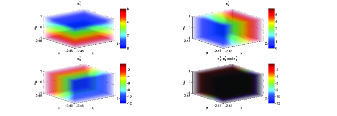
Figure 1: $C_{1}$

IV.2 Critical Point $C_{2}$

For critical point $C_{2}$, $A^{2}=\left(\begin{array}[]{c}-1\\ 0\\ 1\\ \end{array}\right)$ and the Jacobian matrix of the system (14)-(16) at this critical point has the characteristic polynomial

$$a^{2}_{3}s^{3}+a^{2}_{2}s^{2}+a^{2}_{1}s+a^{2}_{0}=0$$ (24)

where

$$a^{2}_{3}=1,a^{2}_{2}=(-3\omega_{m}+\frac{\sqrt{6}\lambda}{2}+\sqrt{6}\mu+6)$$ (25)

and

$$a^{2}_{1}=[-\frac{(3\omega_{m}-3)(\sqrt{6}\lambda-6)}{2}+\frac{(6\omega_{m}-\sqrt{6}\lambda)(\sqrt{6}\mu+6)}{2}],a^{2}_{0}=-\frac{(3\omega_{m}-3)(\sqrt{6}\lambda-6)(\sqrt{6}\mu+6)}{2}.$$ (26)

This has eigen values as

$$e^{2}_{1}=3\omega_{m}-3,e^{2}_{2}=3-\frac{\sqrt{6}\lambda}{2},e^{2}_{3}=-\sqrt{6}\mu-6.$$ (27)

We again note that for the situation where $\omega_{m}=1,\lambda=\sqrt{6}$ and $\mu=-\sqrt{6},$ the center manifold reduction fails as all the three eigenvalues are zero in this case too.

We present the TABLE 5 containing the non-hyperbolic subcases and the result of their stability analysis :

Table 5: $C_{2}$(Center Manifolds and Reduced System)

Case	$\omega_{m}$	$\lambda$	$\mu$	Center Manifold	Reduced System
a	$1$	NA	NA	$\bar{\bar{y}}=O(\bar{\bar{x}}^{3}),\bar{\bar{\nu}}=O(\bar{\bar{x}}^{3})$	$\bar{\bar{x}}^{\prime}=0$
b	NA	$\sqrt{6}$	NA	$\bar{\bar{y}}=\frac{1}{2}\bar{\bar{x}}^{2}+O(\bar{\bar{x}}^{3}),\bar{\bar{\nu}}=O(\bar{\bar{x}}^{3})$	$\bar{\bar{x}}^{\prime}=-\frac{3}{2}\bar{\bar{x}}^{3}$
c	NA	NA	$-\sqrt{6}$	$\bar{\bar{y}}=O(\bar{\bar{x}}^{3}),\bar{\bar{\nu}}=O(\bar{\bar{x}}^{3})$	$\bar{\bar{x}}^{\prime}=-\frac{3}{2}\bar{\bar{x}}^{2}$
d	$1$	$\sqrt{6}$	NA	$\bar{\bar{\nu}}=O(||(\bar{\bar{x}},\bar{\bar{y}})||^{3})$	$\bar{\bar{x}}^{\prime}=-3\bar{\bar{x}}\bar{\bar{y}}^{2},\bar{\bar{y}}^{\prime}=3\bar{\bar{x}}\bar{\bar{y}}$
e	$1$	NA	$-\sqrt{6}$	$\bar{\bar{\nu}}=O(||(\bar{\bar{x}},\bar{\bar{y}})||^{3})$	$\bar{\bar{x}}^{\prime}=3\bar{\bar{x}}\bar{\bar{y}},\bar{\bar{y}}^{\prime}=-6\bar{\bar{x}}\bar{\bar{y}}-\frac{3}{2}\bar{\bar{y}}^{2}$
f	NA	$\sqrt{6}$	$-\sqrt{6}$	$\bar{\bar{\nu}}=\frac{1}{2}\bar{\bar{x}}^{2}+O(||(\bar{\bar{x}},\bar{\bar{y}})||^{3})$	$\bar{\bar{x}}^{\prime}=\frac{3}{4}\bar{\bar{x}}\bar{\bar{y}},\bar{\bar{y}}^{\prime}=-\frac{3}{2}\bar{\bar{y}}^{2}$

For subcase (a), the $P^{2}_{a}$ is $\left(\begin{array}[]{ccc}1&0&0\\ 0&1&0\\ 0&0&1\\ \end{array}\right).$

For subcase (b), $P^{2}_{b}=\left(\begin{array}[]{ccc}0&1&0\\ 1&0&0\\ 0&0&1\\ \end{array}\right).$

For subcase (c), $P^{2}_{c}=\left(\begin{array}[]{ccc}0&1&0\\ 0&0&1\\ 1&0&0\\ \end{array}\right).$

For subcase (d), $P^{2}_{d}=\left(\begin{array}[]{ccc}1&0&0\\ 0&1&0\\ 0&0&1\\ \end{array}\right).$

For subcase (e), $P^{2}_{e}=\left(\begin{array}[]{ccc}1&0&0\\ 0&0&1\\ 0&1&0\\ \end{array}\right).$

For subcase (f), $P^{2}_{f}=\left(\begin{array}[]{ccc}0&0&1\\ 1&0&0\\ 0&1&0\\ \end{array}\right).$

We summarize our results for the stability of the reduced system of $C_{2}$ in the TABLE 6.

Table 6: Summary for the critical point $C_{2}$(non-hyperbolic cases)

Case	$\omega_{m}$	$\lambda$	$\mu$	Stability(RS)
a	$1$	NA	NA	ND
b	NA	$\sqrt{6}$	NA	Stable
c	NA	NA	$-\sqrt{6}$	Stable
d	$1$	$\sqrt{6}$	NA	Stable
e	$1$	NA	$-\sqrt{6}$	Unstable
f	NA	$\sqrt{6}$	$-\sqrt{6}$	Unstable

Where we come to the conclusion as above by solving the ODE/pair of ODEs of the simplified reduced system. In the subcase (a), the center manifold analysis fails again to determine stability as the reduced system represents a center. Hence some higher dimensional analysis may be needed to determine the stability for this subcase. In the subcase (e), we found that the solution of the system of ODEs that govern the reduced dynamics for $C_{2}$ is sensitive to initial conditions, it is chaotic in nature indeed.

FIG.2 represents the stability analysis for $C_{2}$ for different values of parameters in all the possible cases. In FIG.2, the stability of $C_{2}$ in the parameter region $\{-1\leq\omega_{m}\leq 1,-\sqrt{6}\leq\lambda\leq\sqrt{6},-\sqrt{6}\leq\mu\leq\sqrt{6}\}$ has been considered.

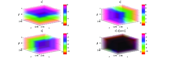
Figure 2: $C_{2}$

IV.3 Critical Point $C_{3}$

For $C_{3}$ the $A^{3}=\left(\begin{array}[]{c}1\\ 0\\ \frac{\mu^{2}}{3}-1\\ \end{array}\right).$

The Jacobian matrix of the system (14)-(16) at this point has the characteristic polynomial

$$a^{3}_{3}s^{3}+a^{3}_{2}s^{2}+a^{3}_{1}s+a^{3}_{0}=0$$ (28)

where

$$a^{3}_{3}=1,$$ (29)

$$a^{3}_{2}=\frac{108\mu-36\omega_{m}\mu^{3}-45\mu^{2}+54\omega_{m}\mu+9\lambda\mu^{2}-3\lambda\mu^{4}+6\omega_{m}\mu^{5}+9\mu^{3}}{2\mu(\mu^{2}-3)^{2}},$$ (30)

$$a^{3}_{1}=X3-Y3$$ (31)

where

$$X3=\frac{27\lambda\mu+27\omega_{m}\mu^{2}-9\omega_{m}\mu^{4}+27\mu^{2}-9\lambda\omega_{m}\mu^{3}+27\lambda\omega_{m}\mu}{2(\mu^{2}-3)^{2}}$$ (32)

and

$$Y3=\frac{3(54\mu-27\mu^{3}+3\mu^{5})(6\omega_{m}+\lambda\mu-2\omega_{m}\mu^{2}+\mu^{2}+6)}{4\mu(\mu^{2}-3)^{3}}$$ (33)

and

$$a^{3}_{0}=\frac{3(\lambda+\mu)(-3\omega_{m}\mu^{2}+9\omega_{m}+9)(54\mu-27\mu^{3}+3\mu^{5})}{4(\mu^{2}-3)^{4}}.$$ (34)

In this case,

$$e^{3}_{1}=\frac{3}{\frac{\mu^{2}}{3}-1}-3\omega_{m},$$ (35)

$$e^{3}_{2}=\frac{3(\mu^{2}+\lambda\mu)}{2(\mu^{2}-3)}$$ (36)

and

$$e^{3}_{3}=\frac{3(-18+9\mu^{2}-\mu^{4})}{2(\mu^{2}-3)^{2}}.$$ (37)

$e^{3}_{1}$ is zero if $\mu=\sqrt{3(1+\frac{1}{\omega_{m}})},$ $e^{3}_{2}$ is zero if $\mu=-\lambda,$ where $\lambda<0,$ whereas $e^{3}_{3}$ is always non-zero for $C_{3}$. $e^{3}_{1}$ and $e^{3}_{2}$ are both zero if $\omega_{m}=\frac{3}{\lambda^{2}-3},$ where $\lambda<0.$

We present the TABLE 7 containing the non-hyperbolic subcases and their stability.

Table 7: $C_{3}$(Cases)

Case	$\omega_{m}$	$\lambda$	$\mu$
a	NA	NA	$\sqrt{3(1+\frac{1}{\omega_{m}})}$
b	NA	$\lambda<0$	$\mu=-\lambda$
c	$\omega_{m}=\frac{3}{\lambda^{2}-3}$	$\lambda<0$	NA

The center manifolds and the reduced systems are described in the TABLE 8.

Table 8: $C_{3}$(Center Manifolds and Reduced System)

Case	Center Manifold	Reduced System
a	$\bar{\bar{y}}=0,\bar{\bar{\nu}}=C^{3,a}_{2,(2,0,0)}\bar{\bar{x}}^{2}$	$\bar{\bar{x}}^{\prime}=R^{3,a}_{1,(2,0,0)}\bar{\bar{x}}^{2}$
b	$\bar{\bar{y}}=C^{3,b}_{1,(2,0,0)}\bar{\bar{x}}^{2},\bar{\bar{\nu}}=C^{3,b}_{2,(2,0,0)}\bar{\bar{x}}^{2}$	$\bar{\bar{x}}^{\prime}=R^{3,b}_{1,(5,0,0)}\bar{\bar{x}}^{5}$
c	$\bar{\bar{\nu}}=C^{3,c}_{1,(2,0,0)}\bar{\bar{x}}^{2}+C^{3,c}_{1,(0,2,0)}\bar{\bar{y}}^{2}$	$\bar{\bar{x}}^{\prime}=R^{3,c}_{1,(1,2,0)}\bar{\bar{x}}\bar{\bar{y}}^{2},\bar{\bar{y}}^{\prime}=R^{3,c}_{2,(0,2,0)}\bar{\bar{y}}^{2}$

where

$$C^{3,a}_{2,(2,0,0)}=-\frac{\omega_{m}(8\omega_{m}^{2}+7\omega_{m}+1)}{4(\omega_{m}^{2}-1)},R^{3,a}_{1,(2,0,0)}=-\frac{3}{2}\omega_{m}^{2}$$ (38)

and

$$C^{3,b}_{1,(2,0,0)}=-\frac{\lambda^{2}(\lambda^{2}-6)}{3(6\omega_{m}-2\lambda^{2}\omega_{m}+\lambda^{2})},C^{3,b}_{2,(2,0,0)}=-\frac{2\lambda^{2}(\lambda^{2}-3)(\omega_{m}-1)}{3(6\omega_{m}-2\lambda^{2}\omega_{m}+\lambda^{2})}$$ (39)

and

$$R^{3,b}_{1,(5,0,0)}=\frac{3(6\omega_{m}-2\lambda^{2}\omega_{m}-5\lambda^{2}+6)}{16(\lambda^{2}-3)}.$$ (40)

Also,

$$C^{3,c}_{1,(2,0,0)}=\frac{2\lambda^{2}}{3},C^{3,c}_{1,(0,2,0)}=\frac{12(\lambda^{2}-3)(2916\lambda^{2}-972\lambda^{4}-1215\lambda^{6}+756\lambda^{8}-126\lambda^{10}+\lambda^{14})}{16\lambda^{4}(\lambda^{2}-3)^{5}(\lambda^{2}-6)^{2}}$$ (41)

and

$$R^{3,c}_{1,(1,2,0)}=-\frac{27(-5832\lambda^{3}+6804\lambda^{5}-2916\lambda^{7}+540\lambda^{9}-36\lambda^{11})}{4\lambda^{5}(\lambda^{2}-3)^{5}(\lambda^{2}-6)^{2}},R^{3,c}_{2,(0,2,0)}=-\frac{27}{(\lambda^{2}-3)^{2}}.$$ (42)

For subcase (a), $P^{3}_{a}$ is $\left(\begin{array}[]{ccc}\frac{\omega_{m}}{2(\omega_{m}+1)}&0&0\\ 0&1&0\\ 1&0&1\\ \end{array}\right).$

For subcase (b), $P^{3}_{b}=\left(\begin{array}[]{ccc}0&\frac{3(6\omega_{m}-2\lambda^{2}\omega_{m}+\lambda^{2})}{2\lambda^{2}(\lambda^{2}-6)}&0\\ 1&0&0\\ 0&1&1\\ \end{array}\right).$

For subcase (c), $P^{3}_{c}=\left(\begin{array}[]{ccc}0&\frac{3(18\lambda-9\lambda^{3}+\lambda^{5})}{2\lambda^{3}(\lambda^{2}-3)(\lambda^{2}-6)}&0\\ 1&0&0\\ 0&1&1\\ \end{array}\right).$

We summarize our results for the stability of the reduced system of $C_{3}$ in the TABLE 9.

Table 9: Summary for the critical point $C_{3}$(non-hyperbolic cases)

Case	$\omega_{m}$	$\lambda$	$\mu$	Stability (RS)
a	NA	NA	$\sqrt{3(1+\frac{1}{\omega_{m}})}$	Stable
b	NA	$\lambda<0$	$\mu=-\lambda$	Stable
c	$\omega_{m}=\frac{3}{\lambda^{2}-3}$	$\lambda<0$	NA	Unstable

We notice that in the subcase (b) if $\omega_{m}=\frac{5\lambda^{2}-6}{6-2\lambda^{2}},$ then the center manifold reduction fails as $R^{3,b}_{1,(5,0,0)}=0.$ In this case, some higher degree center manifold reduction is necessary. Case (c) is interesting in a sense that though it is unstable, it does not diverge to infinity, rather converges to some point other than $C_{3}$ in the neighborhood of its initial position parallel to $\bar{\bar{y}}$ axis.

Lastly we present the FIG.3 to show the stability analysis for $C_{3}$ for different values of parameters in all the possible cases (both the hyperbolic and the non-hyperbolic). In the FIG.3 the stability of $C_{3}$ in the region $\{0\leq\omega_{m}\leq 1,\sqrt{6}\leq\lambda\leq\sqrt{6}+1,-\sqrt{6}-1\leq\mu\leq-\sqrt{6}\}$ of the parameter space has been presented.

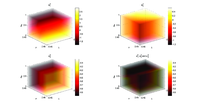
Figure 3: $C_{3}$

IV.4 Critical Point $C_{4}$

For $C_{4}$ the $A^{4}=\left(\begin{array}[]{c}-1\\ 0\\ \frac{\mu^{2}}{3}-1\\ \end{array}\right).$

The Jacobian matrix of the system (14)-(16) has the characteristic polynomial at this point as

$$a^{4}_{3}s^{3}+a^{4}_{2}s^{2}+a^{4}_{1}s+a^{4}_{0}=0$$ (43)

where

$$a^{4}_{3}=1,$$ (44)

$$a^{4}_{2}=\frac{108\mu-36\omega_{m}\mu^{3}-45\mu^{2}+54\omega_{m}\mu+9\lambda\mu^{2}-3\lambda\mu^{4}+6\omega_{m}\mu^{5}+9\mu^{3}}{2\mu(\mu^{2}-3)^{2}},$$ (45)

$$a^{4}_{1}=X4-Y4$$ (46)

where

$$X4=\frac{27\lambda\mu+27\omega_{m}\mu^{2}-9\omega_{m}\mu^{4}+27\mu^{2}-9\lambda\omega_{m}\mu^{3}+27\lambda\omega_{m}\mu}{2(\mu^{2}-3)^{2}}$$ (47)

and

$$Y4=\frac{3(54\mu-27\mu^{3}+3\mu^{5})(6\omega_{m}+\lambda\mu-2\omega_{m}\mu^{2}+\mu^{2}+6)}{4\mu(\mu^{2}-3)^{3}}$$ (48)

and

$$a^{4}_{0}=\frac{3(\lambda+\mu)(-3\omega_{m}\mu^{2}+9\omega_{m}+9)(54\mu-27\mu^{3}+3\mu^{5})}{4(\mu^{2}-3)^{4}}.$$ (49)

The eigen values are

$$e^{4}_{1}=\frac{3}{\frac{\mu^{2}}{3}-1}-3\omega_{m},$$ (50)

$$e^{4}_{2}=\frac{3(\mu^{2}+\lambda\mu)}{2(\mu^{2}-3)}$$ (51)

and

$$e^{4}_{3}=\frac{3(-18+9\mu^{2}-\mu^{4})}{2(\mu^{2}-3)^{2}}.$$ (52)

$e^{4}_{1}$ is zero if $\mu=-\sqrt{3(1+\frac{1}{\omega_{m}})},$ $e^{4}_{2}$ is zero if $\mu=-\lambda,$ where $\lambda>0,$ whereas $e^{4}_{3}$ is always non-zero for $C_{4}$. $e^{4}_{1}$ and $e^{4}_{2}$ are both zero if $\omega_{m}=\frac{3}{\lambda^{2}-3},$ where $\lambda>0.$

We present the TABLE 10 containing the non-hyperbolic subcases and their stability.

Table 10: $C_{4}$(Cases)

Case	$\omega_{m}$	$\lambda$	$\mu$
a	NA	NA	$-\sqrt{3(1+\frac{1}{\omega_{m}})}$
b	NA	$\lambda>0$	$\mu=-\lambda$
c	$\omega_{m}=\frac{3}{\lambda^{2}-3}$	$\lambda>0$	NA

The center manifolds and the reduced systems are described in the TABLE 11.

Table 11: $C_{4}$(Center Manifolds and Reduced System)

Case	Center Manifold	Reduced System
a	$\bar{\bar{y}}=0,\bar{\bar{\nu}}=C^{4,a}_{2,(2,0,0)}\bar{\bar{x}}^{2}$	$\bar{\bar{x}}^{\prime}=R^{4,a}_{1,(2,0,0)}\bar{\bar{x}}^{2}$
b	$\bar{\bar{y}}=C^{4,b}_{1,(2,0,0)}\bar{\bar{x}}^{2},\bar{\bar{\nu}}=C^{4,b}_{2,(2,0,0)}\bar{\bar{x}}^{2}$	$\bar{\bar{x}}^{\prime}=R^{4,b}_{1,(5,0,0)}\bar{\bar{x}}^{5}$
c	$\bar{\bar{\nu}}=C^{4,c}_{1,(2,0,0)}\bar{\bar{x}}^{2}+C^{4,c}_{1,(0,2,0)}\bar{\bar{y}}^{2}$	$\bar{\bar{x}}^{\prime}=R^{4,c}_{1,(1,2,0)}\bar{\bar{x}}\bar{\bar{y}}^{2},\bar{\bar{y}}^{\prime}=R^{4,c}_{2,(0,2,0)}\bar{\bar{y}}^{2}$

where

$$C^{4,a}_{2,(2,0,0)}=-\frac{\omega_{m}(8\omega_{m}^{2}+7\omega_{m}+1)}{4(\omega_{m}^{2}-1)},R^{4,a}_{1,(2,0,0)}=-3\omega_{m}^{2}$$ (53)

and

$$C^{4,b}_{1,(2,0,0)}=-\frac{\lambda^{2}(\lambda^{2}-6)}{3(6\omega_{m}-2\lambda^{2}\omega_{m}+\lambda^{2})},C^{4,b}_{2,(2,0,0)}=-\frac{2\lambda^{2}(\lambda^{2}-3)(\omega_{m}-1)}{3(6\omega_{m}-2\lambda^{2}\omega_{m}+\lambda^{2})}$$ (54)

and

$$R^{4,b}_{1,(5,0,0)}=\frac{3(6\omega_{m}-2\lambda^{2}\omega_{m}-5\lambda^{2}+6)}{16(\lambda^{2}-3)}.$$ (55)

Also,

$$C^{4,c}_{1,(2,0,0)}=\frac{2\lambda^{2}}{3},C^{4,c}_{1,(0,2,0)}=\frac{3(\lambda^{4}+15\lambda^{2}+18)}{4\lambda^{2}(\lambda^{4}-9\lambda^{2}+18)}$$ (56)

and

$$R^{4,c}_{1,(1,2,0)}=\frac{243}{\lambda^{2}(\lambda^{2}-3)^{2}(\lambda^{2}-6)},R^{4,c}_{2,(0,2,0)}=-\frac{27}{(\lambda^{2}-3)^{2}}.$$ (57)

For subcase (a), $P^{4}_{a}$ is $\left(\begin{array}[]{ccc}-\frac{\omega_{m}}{2(\omega_{m}+1)}&0&0\\ 0&1&0\\ 1&0&1\\ \end{array}\right).$

For subcase (b), $P^{4}_{b}=\left(\begin{array}[]{ccc}0&-\frac{3(6\omega_{m}-2\lambda^{2}\omega_{m}+\lambda^{2})}{2\lambda^{2}(\lambda^{2}-6)}&0\\ 1&0&0\\ 0&1&1\\ \end{array}\right).$

For subcase (c), $P^{4}_{c}=\left(\begin{array}[]{ccc}0&-\frac{3}{2\lambda^{2}}&0\\ 1&0&0\\ 0&1&1\\ \end{array}\right).$

In the TABLE 12, we summarize our results for the stability of the reduced system of $C_{4}.$

Table 12: Summary for the critical point $C_{4}$(non-hyperbolic cases)

Case	$\omega_{m}$	$\lambda$	$\mu$	Stability (RS)
a	NA	NA	$-\sqrt{3(1+\frac{1}{\omega_{m}})}$	Stable
b	NA	$\lambda>0$	$\mu=-\lambda$	Stable
c	$\omega_{m}=\frac{3}{\lambda^{2}-3}$	$\lambda>0$	NA	Unstable

Again here we notice that in the subcase (b) if $\omega_{m}=\frac{5\lambda^{2}-6}{6-2\lambda^{2}},$ then the center manifold reduction fails as $R^{4,b}_{1,(5,0,0)}=0.$ So, some higher degree center manifold reduction is necessary. Case (c) is again interesting because although it is unstable, it does not diverge to infinity, rather converges to some point other than $C_{4}$ in the neighborhood of its initial position parallel to $\bar{\bar{y}}$ axis.

Next we present the FIG.4 to show the stability analysis for $C_{4}$ for different values of parameters in all the possible cases to end this subsection. We note that in the FIG.4, we took $\{0\leq\omega_{m}\leq 1,\sqrt{6}\leq\lambda\leq\sqrt{6}+1,-\sqrt{6}-1\leq\mu\leq-\sqrt{6}\}$ as our parameter space.

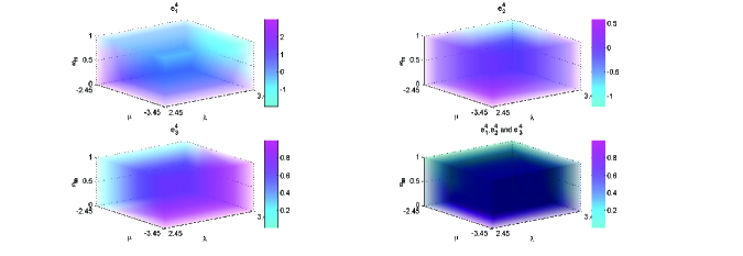
Figure 4: $C_{4}$

IV.5 Critical Point $C_{5}$

For $C_{5}$ the $A^{5}=\left(\begin{array}[]{c}\frac{\sqrt{3(1+\frac{1}{\omega_{m}})}}{\mu}\\ 0\\ \frac{1}{\omega_{m}}\\ \end{array}\right).$

The Jacobian matrix of the system (14)-(16) at $C_{5}$ has the characteristic polynomial as :

$$a^{5}_{3}s^{3}+a^{5}_{2}s^{2}+a^{5}_{1}s+a^{5}_{0}=0$$ (58)

where

$$a^{5}_{3}=1,$$ (59)

$$a^{5}_{2}=-[\frac{3\mu^{2}(\omega_{m}-1)}{2\mu^{2}}+\frac{3(\lambda+\mu+\omega_{m}\lambda+\omega_{m}\mu)}{2\mu}],$$ (60)

$$a^{3}_{1}=X5+Y5$$ (61)

where

$$X5=\frac{(\omega_{m}+1)(27-27\omega_{m}^{2}-9\omega_{m}\mu^{2}+9\omega_{m}^{2}\mu^{2})}{2\mu^{2}}$$ (62)

and

$$Y5=\frac{9(\omega_{m}-1)(\lambda+\mu+\lambda\omega_{m}+\omega_{m}\mu)}{4\mu}$$ (63)

and

$$a^{5}_{0}=-\frac{3(\lambda+\mu+\omega_{m}\lambda+\omega_{m}\mu)(\omega_{m}+1)(27-27\omega_{m}^{2}-9\omega_{m}\mu^{2}+9\omega_{m}^{2}\mu^{2})}{4\mu^{3}}.$$ (64)

Here,

$$e^{5}_{1}=\frac{3(\omega_{m}\mu-\mu+\sqrt{(1-\omega_{m})(8\omega_{m}^{2}\mu^{2}+7\omega_{m}\mu^{2}-24\omega_{m}^{2}+\mu^{2}-48\omega_{m}-24)})}{4\mu},$$ (65)

$$e^{5}_{2}=\frac{3(\omega_{m}\mu-\mu-\sqrt{(1-\omega_{m})(8\omega_{m}^{2}\mu^{2}+7\omega_{m}\mu^{2}-24\omega_{m}^{2}+\mu^{2}-48\omega_{m}-24)})}{4\mu}$$ (66)

and

$$e^{5}_{3}=\frac{3(1+\omega_{m})(\lambda+\mu)}{2\mu}.$$ (67)

$e^{5}_{1}$ and $e^{5}_{2}$ are both zero if $\mu=\sqrt{3(1+\frac{1}{\omega_{m}})}$ or if $\mu=-\sqrt{3(1+\frac{1}{\omega_{m}})}.$ But then $C_{5}$ coinsides with $C_{3}$ in the first case and with $C_{4}$ in the second case. $e^{5}_{3}$ is zero if $\mu=-\lambda$ where $\lambda\neq 0.$ So this is the only new case.

For this case, the center manifold and the reduced system are described in the TABLE 13.

Table 13: $C_{5}$(Center Manifolds and Reduced System)

Case	Center Manifold	Reduced System
a	$\bar{\bar{y}}=C^{5,a}_{1,(2,0,0)}\bar{\bar{x}}^{2},\bar{\bar{\nu}}=C^{5,a}_{2,(2,0,0)}\bar{\bar{x}}^{2}$	$\bar{\bar{x}}^{\prime}=R^{5,a}_{1,(5,0,0)}\bar{\bar{x}}^{5}$

where

$$C^{5,a}_{1,(2,0,0)}=-\frac{\lambda^{2}(\lambda+3\omega_{m}\lambda-4\lambda\omega_{m}^{2}+Z5)}{6\omega_{m}Z5},C^{5,a}_{2,(2,0,0)}=\frac{\lambda^{2}(\lambda+3\omega_{m}\lambda-4\lambda\omega_{m}^{2}-Z5)}{6\omega_{m}Z5}$$ (68)

and

$$R^{5,a}_{1,(5,0,0)}=-\frac{(4\lambda^{4}\omega_{m}+24\lambda^{2}\omega_{m}^{2}+24\lambda^{2}\omega_{m}+\lambda^{4})}{48(1+\omega_{m})}.$$ (69)

Here $Z5=\sqrt{(1-\omega_{m})(8\omega_{m}^{2}\lambda^{2}+7\omega_{m}\lambda^{2}-24\omega_{m}^{2}+\lambda^{2}-48\omega_{m}-24)}.$

For this subcase, $P^{5}_{a}$ is $\left(\begin{array}[]{ccc}0&\frac{\sqrt{3\omega_{m}(1+\omega_{m})}(\lambda-\lambda\omega_{m}+Z5)}{4\lambda^{2}(\omega_{m}^{2}-1)}&\frac{\sqrt{3\omega_{m}(1+\omega_{m})}(\lambda-\lambda\omega_{m}-Z5)}{4\lambda^{2}(\omega_{m}^{2}-1)}\\ 1&0&0\\ 0&1&1\\ \end{array}\right).$

We summarize our results for the stability of the reduced system of $C_{5}$ in the TABLE 14.

Table 14: Summary for the critical point $C_{5}$(non-hyperbolic cases)

Case	$\omega_{m}$	$\lambda$	$\mu$	Stability (RS)
a	NA	$\lambda\neq 0$	$-\lambda$	Stable

Now we present FIG.5 showing the stability analysis for $C_{5}$ for different values of parameters to conclude this subsection. In the FIG.5, the values of the parameters have been restricted in the region $\{0\leq\omega_{m}\leq 1,-\sqrt{6}\leq\lambda\leq\sqrt{6},5\leq\mu\leq 6\}.$

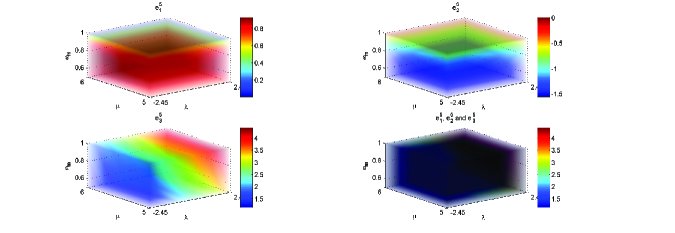
Figure 5: $C_{5}$

IV.6 Critical Point $C_{6}$

For $C_{6}$ the $A^{6}=\left(\begin{array}[]{c}-\frac{\sqrt{3(1+\frac{1}{\omega_{m}})}}{\mu}\\ 0\\ \frac{1}{\omega_{m}}\\ \end{array}\right).$

The Jacobian matrix of the system (14)-(16) at $C_{6}$ has the characteristic polynomial as the following :

$$a^{6}_{3}s^{3}+a^{6}_{2}s^{2}+a^{6}_{1}s+a^{6}_{0}=0$$ (70)

where

$$a^{6}_{3}=1,$$ (71)

$$a^{6}_{2}=\frac{3(4\mu\omega_{m}^{2}+2\mu+\omega_{m}\lambda+\lambda)}{2\mu},$$ (72)

$$a^{6}_{1}=\frac{9(1+\omega_{m})(-6\omega_{m}^{2}\mu^{2}+4\lambda\omega_{m}^{2}\mu+6\omega_{m}^{2}+\omega_{m}\mu^{2}+\lambda\omega_{m}\mu-3\mu^{2}+3\lambda\mu-6)}{4\mu^{2}}$$ (73)

and

$$a^{6}_{0}=\frac{27(\omega_{m}^{2}-1)(\lambda-\mu)(\omega_{m}+1)(-\omega_{m}\mu^{2}+3\omega_{m}+3)}{4\mu^{3}}.$$ (74)

Then,

$$e^{6}_{1}=-\frac{3(3\mu+\omega_{m}\mu+4\omega_{m}^{2}\mu+Y6)}{4\mu},$$ (75)

$$e^{6}_{2}=-\frac{3(3\mu+\omega_{m}\mu+4\omega_{m}^{2}\mu-Y6)}{4\mu}$$ (76)

and

$$e^{6}_{3}=-\frac{3(1+\omega_{m})(\lambda-\mu)}{2\mu}.$$ (77)

Where $Y6=\sqrt{(16\omega_{m}^{4}\mu^{2}+16\omega_{m}^{3}\mu^{2}-24\omega_{m}^{3}+25\omega_{m}^{2}\mu^{2}-24\omega_{m}^{2}-2\omega_{m}\mu^{2}+24\omega_{m}+9\mu^{2}+24)}.$

Here again, $e^{6}_{1}$ and $e^{6}_{2}$ are both zero if $\mu=\sqrt{3(1+\frac{1}{\omega_{m}})}$ or if $\mu=-\sqrt{3(1+\frac{1}{\omega_{m}})}.$ But then $C_{6}$ coinsides with $C_{4}$ in the first case and with $C_{3}$ in the second case. $e^{6}_{3}$ is zero if $\mu=\lambda$ where $\lambda\neq 0.$ But this case also identical with subcase (a) of $C_{5}.$ So no new case arise with $C_{6}.$

We present FIG.6 showing the stability analysis for $C_{6}$ for different values of parameters for the possible cases and conclude this subsection. It is to be noted that the parameter space in the FIG.6 is $\{0\leq\omega_{m}\leq 1,-\sqrt{6}\leq\lambda\leq\sqrt{6},5\leq\mu\leq 6\}.$

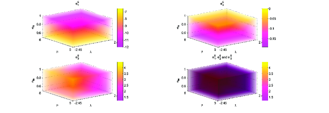
Figure 6: $C_{6}$

IV.7 Critical Point $C_{7}$

For $C_{7}$ the $A^{7}=\left(\begin{array}[]{c}-\frac{\lambda}{\sqrt{6}}\\ \sqrt{\frac{6-\lambda^{2}}{6}}\\ 1\\ \end{array}\right).$

The Jacobian matrix of the system (14)-(16) has the characteristic polynomial at this point as

$$a^{7}_{3}s^{3}+a^{7}_{2}s^{2}+a^{7}_{1}s+a^{7}_{0}=0$$ (78)

where

$$a^{7}_{3}=1,$$ (79)

$$a^{7}_{2}=-\frac{\lambda^{2}}{2}+\mu\lambda+3\omega_{m}+6,$$ (80)

$$a^{7}_{1}=9\omega_{m}+6\lambda\mu+\frac{3\lambda^{2}\omega_{m}}{2}-\frac{3\lambda^{3}\mu}{2}+\frac{3\lambda^{2}}{2}-\lambda^{4}+3\lambda\omega_{m}\mu+9$$ (81)

and

$$a^{7}_{0}=-\frac{\lambda(\lambda^{2}-6)(\lambda+\mu)(-\lambda^{2}+3\omega_{m}+3)}{2}.$$ (82)

The eigen values are

$$e^{7}_{1}=\frac{\lambda^{2}}{2}-3,$$ (83)

$$e^{7}_{2}=-\lambda(\lambda+\mu)$$ (84)

and

$$e^{7}_{3}=\lambda^{2}-3\omega_{m}-3.$$ (85)

$e^{7}_{1}$ is never zero for $C_{7}$. $e^{7}_{2}$ is zero if $\mu=-\lambda,$ where $e^{7}_{3}$ is zero for $\omega_{m}=\frac{\lambda^{2}}{3}-1$. $e^{7}_{2}$ and $e^{7}_{3}$ are both zero if $\mu=-\lambda$ and $\omega_{m}=\frac{\lambda^{2}}{3}-1$ hold together.

We present the TABLE 15 containing the non-hyperbolic subcases and their stability.

Table 15: $C_{7}$(Cases)

Case	$\omega_{m}$	$\lambda$	$\mu$
a	NA	$|\lambda|<\sqrt{6},\lambda\neq 0$	$-\lambda$
b	$\frac{\lambda^{2}}{3}-1$	$|\lambda|<\sqrt{6},\lambda\neq 0$	NA
c	$\frac{\lambda^{2}}{3}-1$	$|\lambda|<\sqrt{6},\lambda\neq 0$	$-\lambda$

The center manifolds and the reduced systems are described in the TABLE 16.

Table 16: $C_{7}$(Center Manifolds and Reduced System)

Case	Center Manifold	Reduced System
a	$\bar{\bar{y}}=C^{7,a}_{1,(2,0,0)}\bar{\bar{x}}^{2},\bar{\bar{\nu}}=C^{7,a}_{2,(2,0,0)}\bar{\bar{x}}^{2}$	$\bar{\bar{x}}^{\prime}=R^{7,a}_{1,(4,0,0)}\bar{\bar{x}}^{4}$
b	$\bar{\bar{y}}=C^{7,b}_{1,(2,0,0)}\bar{\bar{x}}^{2},\bar{\bar{\nu}}=0$	$\bar{\bar{x}}^{\prime}=R^{7,b}_{1,(2,0,0)}\bar{\bar{x}}^{2}$
c	$\bar{\bar{\nu}}=C^{7,c}_{1,(2,0,0)}\bar{\bar{x}}^{2}+C^{7,c}_{1,(1,1,0)}\bar{\bar{x}}\bar{\bar{y}}+C^{7,c}_{1,(0,2,0)}\bar{\bar{y}}^{2}$	$\bar{\bar{x}}^{\prime}=R^{7,c}_{1,(2,0,0)}\bar{\bar{x}}^{2}+R^{7,c}_{1,(1,1,0)}\bar{\bar{x}}\bar{\bar{y}}+R^{7,c}_{1,(0,2,0)}\bar{\bar{y}}^{2}$
		$\bar{\bar{y}}^{\prime}=R^{7,c}_{2,(2,1,0)}\bar{\bar{x}}^{2}\bar{\bar{y}}+R^{7,c}_{2,(1,2,0)}\bar{\bar{x}}\bar{\bar{y}}^{2}+R^{7,c}_{2,(0,3,0)}\bar{\bar{y}}^{3}$

where

$$C^{7,a}_{1,(2,0,0)}=-\frac{\sqrt{6}\lambda^{2}(36\omega_{m}-4\lambda^{2}\omega_{m}-8\lambda^{2}+\lambda^{4})}{(6-\lambda^{2})^{\frac{3}{2}}(-64\lambda^{2}+384\omega_{m})},C^{7,a}_{2,(2,0,0)}=-\frac{\sqrt{6}\lambda^{2}\omega_{m}}{32\sqrt{(6-\lambda^{2})}(-\lambda^{2}+6\omega_{m})}$$ (86)

and

$$R^{7,a}_{1,(4,0,0)}=\frac{(18\lambda^{4}-288\lambda^{2}+648)}{128(\lambda^{2}-6)^{2}}.$$ (87)

Then

$$C^{7,b}_{1,(2,0,0)}=-\frac{\sqrt{6}\lambda^{2}(2\lambda^{4}-15\lambda^{2}+18)}{2(\lambda^{2}-3)^{2}(6-\lambda^{2})^{\frac{3}{2}}},R^{7,b}_{1,(2,0,0)}=\frac{\sqrt{6}\lambda^{2}(2\lambda^{2}-12)}{2(\lambda^{2}-3)\sqrt{(6-\lambda^{2})}}.$$ (88)

Also,

$$C^{7,c}_{1,(2,0,0)}=-\frac{\sqrt{6}\lambda^{2}(2\lambda^{4}-15\lambda^{2}+18)}{2(\lambda^{2}-3)^{2}(6-\lambda^{2})^{\frac{3}{2}}},C^{7,c}_{1,(1,1,0)}=\frac{(-2\lambda^{4}+3\lambda^{2})}{4(\lambda^{2}-3)^{2}}$$ (89)

and

$$C^{7,c}_{1,(0,2,0)}=\frac{\sqrt{6}\lambda^{2}(-5\lambda^{6}+9\lambda^{4}+81\lambda^{2}-162)}{192(\lambda^{2}-3)^{2}(6-\lambda^{2})^{\frac{3}{2}}}.$$ (90)

The reduced system coefficients for subcase (c) are :

$$R^{7,c}_{1,(2,0,0)}=\frac{\sqrt{6}\lambda^{2}(2\lambda^{2}-12)}{2(\lambda^{2}-3)\sqrt{(6-\lambda^{2})}},R^{7,c}_{1,(1,1,0)}=-\frac{\lambda^{2}(\lambda^{2}-6)}{2(\lambda^{2}-3)}$$ (91)

and

$$R^{7,c}_{1,(0,2,0)}=\frac{\sqrt{6}\lambda^{4}(6\lambda^{4}-60\lambda^{2}+144)}{192\sqrt{(6-\lambda^{2})}(\lambda^{4}-9\lambda^{2}+18)}$$ (92)

and

$$R^{7,c}_{2,(2,1,0)}=\frac{36\lambda^{2}}{(\lambda^{2}-3)^{2}},R^{7,c}_{2,(1,2,0)}=-\frac{3\lambda^{2}\sqrt{(36-6\lambda^{2})}}{(\lambda^{2}-3)^{2}}$$ (93)

and

$$R^{7,c}_{2,(0,3,0)}=\frac{9\lambda^{4}(\lambda^{2}-4)}{8(\lambda^{2}-3)^{2}(\lambda^{2}-6)}.$$ (94)

For subcase (a), $P^{7}_{a}$ is $\left(\begin{array}[]{ccc}\frac{\sqrt{6}\lambda}{24}&\frac{\sqrt{(6-\lambda^{2})}}{\lambda}&-\frac{\lambda(\omega_{m}-1)}{\omega_{m}\sqrt{(6-\lambda^{2})}}\\ \frac{\sqrt{6}\lambda^{2}}{24\sqrt{(6-\lambda^{2})}}&1&1\\ 1&0&0\\ \end{array}\right).$

For subcase (b), $P^{7}_{b}=\left(\begin{array}[]{ccc}-\frac{\lambda(6-\lambda^{2})^{\frac{3}{2}}}{(\lambda^{4}-9\lambda^{2}+18)}&\frac{\sqrt{(6-\lambda^{2})}}{\lambda}&\frac{\sqrt{6}\lambda(\lambda^{2}-6)}{24(3\lambda^{2}+2\mu\lambda-6)}\\ 1&1&-\frac{\lambda^{2}\sqrt{(36-6\lambda^{2})}}{24(3\lambda^{2}+2\mu\lambda-6)}\\ 0&0&1\\ \end{array}\right).$

For subcase (c), $P^{7}_{c}=\left(\begin{array}[]{ccc}-\frac{\lambda(6-\lambda^{2})^{\frac{3}{2}}}{(\lambda^{4}-9\lambda^{2}+18)}&-\frac{\sqrt{6}\lambda}{8(\lambda^{2}-3)}&\frac{\sqrt{(6-\lambda^{2})}}{\lambda}\\ 1&0&1\\ 0&1&0\\ \end{array}\right).$

In the TABLE 17, we summarize our results for the stability of the reduced system of $C_{7}.$

Table 17: Summary for $C_{7}$(non-hyperbolic cases)

Case	$\omega_{m}$	$\lambda$	$\mu$	Stability (RS)
a	NA	$|\lambda|<\sqrt{6},\lambda\neq 0$	$-\lambda$	Stable
b	$\frac{\lambda^{2}}{3}-1$	$|\lambda|<\sqrt{6},\lambda\neq 0$	NA	Stable
c	$\frac{\lambda^{2}}{3}-1$	$|\lambda|<\sqrt{6},\lambda\neq 0$	$-\lambda$	Unstable

Where the coupled nonlinear system of ODEs representing case (c) is chaotic in nature and hence is unstable. We also observe that when $\lambda=\sqrt{7}-1,\mu=1-\sqrt{7}$ and $\omega_{m}\neq\frac{5-2\sqrt{7}}{3}$ or $\lambda=-\sqrt{7}+1,\mu=-1+\sqrt{7}$ and $\omega_{m}\neq\frac{5-2\sqrt{7}}{3}$ in the subcase (a), then $R^{7,a}_{1,(4,0,0)}=0.$ Therefore we can not decide the stability. Some higher degree center manifold reduction seems to be nesessary.

Next we present FIG.7 showing the stability analysis for $C_{7}$ and end this subsection. The parameter space in the FIG.7 is the set $\{-1\leq\omega_{m}\leq 1,-\sqrt{6}\leq\lambda\leq\sqrt{6},-\sqrt{6}\leq\mu\leq\sqrt{6}\}.$

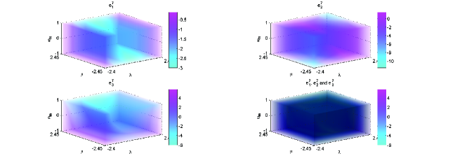
Figure 7: $C_{7}$

IV.8 Critical Point $C_{8}$

For this case, $A^{8}=\left(\begin{array}[]{c}-\frac{\lambda}{\sqrt{6}}\\ -\sqrt{\frac{6-\lambda^{2}}{6}}\\ 1\\ \end{array}\right).$

The Jacobian matrix of the system (14)-(16) has the characteristic polynomial

$$a^{8}_{3}s^{3}+a^{8}_{2}s^{2}+a^{8}_{1}s+a^{8}_{0}=0$$ (95)

where

$$a^{8}_{3}=1,$$ (96)

$$a^{8}_{2}=-\frac{\lambda^{2}}{2}+\mu\lambda+3\omega_{m}+6,$$ (97)

$$a^{8}_{1}=9\omega_{m}+6\lambda\mu+\frac{3\lambda^{2}\omega_{m}}{2}-\frac{3\lambda^{3}\mu}{2}+\frac{3\lambda^{2}}{2}-\lambda^{4}+3\lambda\omega_{m}\mu+9$$ (98)

and

$$a^{8}_{0}=-\frac{\lambda(\lambda^{2}-6)(\lambda+\mu)(-\lambda^{2}+3\omega_{m}+3)}{2}.$$ (99)

The eigen values are

$$e^{8}_{1}=\frac{\lambda^{2}}{2}-3,$$ (100)

$$e^{8}_{2}=-\lambda(\lambda+\mu)$$ (101)

and

$$e^{8}_{3}=\lambda^{2}-3\omega_{m}-3.$$ (102)

$e^{8}_{1}$ is never zero. $e^{8}_{2}$ is zero if $\mu=-\lambda,$ where $e^{8}_{3}$ is zero for $\omega_{m}=\frac{\lambda^{2}}{3}-1$. $e^{8}_{2}$ and $e^{8}_{3}$ are both zero if $\mu=-\lambda$ and $\omega_{m}=\frac{\lambda^{2}}{3}-1$ hold together.

We present the TABLE 18 containing various subcases and their stability.

Table 18: $C_{8}$(Cases)

Case	$\omega_{m}$	$\lambda$	$\mu$
a	NA	$|\lambda|<\sqrt{6},\lambda\neq 0$	$-\lambda$
b	$\frac{\lambda^{2}}{3}-1$	$|\lambda|<\sqrt{6},\lambda\neq 0$	NA
c	$\frac{\lambda^{2}}{3}-1$	$|\lambda|<\sqrt{6},\lambda\neq 0$	$-\lambda$

The center manifolds and the reduced systems are described in the TABLE 19.

Table 19: $C_{8}$(Center Manifolds and Reduced System)

Case	Center Manifold	Reduced System
a	$\bar{\bar{y}}=C^{8,a}_{1,(2,0,0)}\bar{\bar{x}}^{2},\bar{\bar{\nu}}=C^{8,a}_{2,(2,0,0)}\bar{\bar{x}}^{2}$	$\bar{\bar{x}}^{\prime}=R^{8,a}_{1,(4,0,0)}\bar{\bar{x}}^{4}$
b	$\bar{\bar{y}}=C^{8,b}_{1,(2,0,0)}\bar{\bar{x}}^{2},\bar{\bar{\nu}}=0$	$\bar{\bar{x}}^{\prime}=R^{8,b}_{1,(2,0,0)}\bar{\bar{x}}^{2}$
c	$\bar{\bar{\nu}}=C^{8,c}_{1,(2,0,0)}\bar{\bar{x}}^{2}+C^{8,c}_{1,(1,1,0)}\bar{\bar{x}}\bar{\bar{y}}+C^{8,c}_{1,(0,2,0)}\bar{\bar{y}}^{2}$	$\bar{\bar{x}}^{\prime}=R^{8,c}_{1,(2,0,0)}\bar{\bar{x}}^{2}+R^{8,c}_{1,(1,1,0)}\bar{\bar{x}}\bar{\bar{y}}+R^{8,c}_{1,(0,2,0)}\bar{\bar{y}}^{2}$
		$\bar{\bar{y}}^{\prime}=R^{8,c}_{2,(2,1,0)}\bar{\bar{x}}^{2}\bar{\bar{y}}+R^{8,c}_{2,(1,2,0)}\bar{\bar{x}}\bar{\bar{y}}^{2}+R^{8,c}_{2,(0,3,0)}\bar{\bar{y}}^{3}$

where

$$C^{8,a}_{1,(2,0,0)}=\frac{\sqrt{6}\lambda^{2}(36\omega_{m}-4\lambda^{2}\omega_{m}-8\lambda^{2}+\lambda^{4})}{(6-\lambda^{2})^{\frac{3}{2}}(-64\lambda^{2}+384\omega_{m})},C^{8,a}_{2,(2,0,0)}=\frac{\sqrt{6}\lambda^{2}\omega_{m}}{32\sqrt{(6-\lambda^{2})}(-\lambda^{2}+6\omega_{m})}$$ (103)

and

$$R^{8,a}_{1,(4,0,0)}=\frac{(18\lambda^{4}-288\lambda^{2}+648)}{128(\lambda^{2}-6)^{2}}.$$ (104)

Then

$$C^{8,b}_{1,(2,0,0)}=\frac{\sqrt{6}\lambda^{2}(2\lambda^{4}-15\lambda^{2}+18)}{2(\lambda^{2}-3)^{2}(6-\lambda^{2})^{\frac{3}{2}}},R^{8,b}_{1,(2,0,0)}=-\frac{\sqrt{6}\lambda^{2}(2\lambda^{2}-12)}{2(\lambda^{2}-3)\sqrt{(6-\lambda^{2})}}.$$ (105)

Also,

$$C^{8,c}_{1,(2,0,0)}=\frac{\sqrt{6}\lambda^{2}(2\lambda^{4}-15\lambda^{2}+18)}{2(\lambda^{2}-3)^{2}(6-\lambda^{2})^{\frac{3}{2}}},C^{8,c}_{1,(1,1,0)}=\frac{(-2\lambda^{4}+3\lambda^{2})}{4(\lambda^{2}-3)^{2}}$$ (106)

and

$$C^{8,c}_{1,(0,2,0)}=-\frac{\sqrt{6}\lambda^{2}(-5\lambda^{6}+9\lambda^{4}+81\lambda^{2}-162)}{192(\lambda^{2}-3)^{2}(6-\lambda^{2})^{\frac{3}{2}}}.$$ (107)

The reduced system coefficients for subcase (c) are :

$$R^{8,c}_{1,(2,0,0)}=-\frac{\sqrt{6}\lambda^{2}(2\lambda^{2}-12)}{2(\lambda^{2}-3)\sqrt{(6-\lambda^{2})}},R^{8,c}_{1,(1,1,0)}=-\frac{\lambda^{2}(\lambda^{2}-6)}{2(\lambda^{2}-3)}$$ (108)

and

$$R^{8,c}_{1,(0,2,0)}=-\frac{\sqrt{6}\lambda^{4}(6\lambda^{4}-60\lambda^{2}+144)}{192\sqrt{(6-\lambda^{2})}(\lambda^{4}-9\lambda^{2}+18)}$$ (109)

and

$$R^{8,c}_{2,(2,1,0)}=\frac{36\lambda^{2}}{(\lambda^{2}-3)^{2}},R^{8,c}_{2,(1,2,0)}=\frac{3\lambda^{2}\sqrt{(36-6\lambda^{2})}}{(\lambda^{2}-3)^{2}}$$ (110)

and

$$R^{8,c}_{2,(0,3,0)}=\frac{9\lambda^{4}(\lambda^{2}-4)}{8(\lambda^{2}-3)^{2}(\lambda^{2}-6)}.$$ (111)

For subcase (a), $P^{8}_{a}$ is $\left(\begin{array}[]{ccc}\frac{\sqrt{6}\lambda}{24}&-\frac{\sqrt{(6-\lambda^{2})}}{\lambda}&\frac{\lambda(\omega_{m}-1)}{\omega_{m}\sqrt{(6-\lambda^{2})}}\\ -\frac{\sqrt{6}\lambda^{2}}{24\sqrt{(6-\lambda^{2})}}&1&1\\ 1&0&0\\ \end{array}\right).$

For subcase (b), $P^{8}_{b}=\left(\begin{array}[]{ccc}\frac{\lambda(6-\lambda^{2})^{\frac{3}{2}}}{(\lambda^{4}-9\lambda^{2}+18)}&-\frac{\sqrt{(6-\lambda^{2})}}{\lambda}&\frac{\sqrt{6}\lambda(\lambda^{2}-6)}{24(3\lambda^{2}+2\mu\lambda-6)}\\ 1&1&\frac{\lambda^{2}\sqrt{(36-6\lambda^{2})}}{24(3\lambda^{2}+2\mu\lambda-6)}\\ 0&0&1\\ \end{array}\right).$

For subcase (c), $P^{8}_{c}=\left(\begin{array}[]{ccc}\frac{\lambda(6-\lambda^{2})^{\frac{3}{2}}}{(\lambda^{4}-9\lambda^{2}+18)}&-\frac{\sqrt{6}\lambda}{8(\lambda^{2}-3)}&-\frac{\sqrt{(6-\lambda^{2})}}{\lambda}\\ 1&0&1\\ 0&1&0\\ \end{array}\right).$

In the TABLE 20, we summarize our results for the stability of the reduced system of $C_{8}.$

Table 20: Summary for $C_{8}$(non-hyperbolic scenario)

Case	$\omega_{m}$	$\lambda$	$\mu$	Stability (RS)
a	NA	$|\lambda|<\sqrt{6},\lambda\neq 0$	$-\lambda$	Stable
b	$\frac{\lambda^{2}}{3}-1$	$|\lambda|<\sqrt{6},\lambda\neq 0$	NA	Stable
c	$\frac{\lambda^{2}}{3}-1$	$|\lambda|<\sqrt{6},\lambda\neq 0$	$-\lambda$	Unstable

Again we see that for case (c) the dynamical system governing the reduced system of $C_{8}$ is chaotic in nature. It is also observed that in the subcase (a), when $\lambda=\sqrt{7}-1,\mu=1-\sqrt{7}$ and $\omega_{m}\neq\frac{5-2\sqrt{7}}{3}$ or $\lambda=-\sqrt{7}+1,\mu=-1+\sqrt{7}$ and $\omega_{m}\neq\frac{5-2\sqrt{7}}{3}$ , then $R^{8,a}_{1,(4,0,0)}=0.$ Therefore we can’t decide the stability, some higher degree center manifold reduction seems nesessary for this particular case.

We end this subsection after presenting FIG.8 showing the stability analysis for $C_{8}$ for different values of parameters. The parameter space considered in FIG.8 is $\{-1\leq\omega_{m}\leq 1,-\sqrt{6}\leq\lambda\leq\sqrt{6},-\sqrt{6}\leq\mu\leq\sqrt{6}\}.$

Figure 8: $C_{8}$

IV.9 Critical Point $C_{9}$

For this case, $A^{9}=\left(\begin{array}[]{c}-\frac{\sqrt{6}(1+\omega_{m})}{2\lambda}\\ \frac{\sqrt{6(1-\omega_{m}^{2})}}{2\lambda}\\ 1\\ \end{array}\right).$

The jacobian matrix of the system (14)-(16) has the following characteristic polynomial

$$a^{9}_{3}s^{3}+a^{9}_{2}s^{2}+a^{9}_{1}s+a^{9}_{0}=0$$ (112)

where

$$a^{9}_{3}=1,$$ (113)

$$a^{9}_{2}=\frac{(9\lambda+6\mu+3\lambda\omega_{m}+6\omega_{m}\mu)}{2\lambda},$$ (114)

$$a^{9}_{1}=\frac{9(\omega_{m}^{2}-1)(-2\lambda^{2}-\mu\lambda+3\omega_{m}+3)}{2\lambda^{2}}$$ (115)

and

$$a^{9}_{0}=\frac{27(\lambda+\mu)(\omega_{m}-1)(\omega_{m}+1)^{2}(-\lambda^{2}+3\omega_{m}+3)}{2\lambda^{3}}.$$ (116)

The eigen values are

$$e^{9}_{1}=\frac{3(\lambda\omega_{m}-\lambda+X9)}{4\lambda},$$ (117)

$$e^{9}_{2}=-\frac{3(\lambda+\mu)(\omega_{m}+1)}{\lambda}$$ (118)

and

$$e^{9}_{3}=\frac{3(\lambda\omega_{m}-\lambda-X9)}{4\lambda},$$ (119)

where

$$X9=\sqrt{(1-\omega_{m})(-9\lambda^{2}\omega_{m}-7\lambda^{2}+24\omega_{m}^{2}+48\omega_{m}+24)}.$$ (120)

$e^{9}_{1}$ and $e^{9}_{3}$ are both zero if $\omega_{m}=1$ or $\omega_{m}=\frac{\lambda^{2}}{3}-1.$ But in the later subcase $C_{9}$ becomes identical with $C_{7}$ or $C_{8}$ depending on whether $\lambda>0$ or $\lambda<0$ respectively. $e^{9}_{2}$ is zero if $\mu=-\lambda.$ Also in the subcase where $\omega_{m}=1$ and $\mu=-\lambda$ both holds, $C_{9}$ becomes identical with $C_{5}$ or $C_{6}$ depending on the sign of $\lambda.$ Hence $\omega_{m}=1$ and $\mu=-\lambda$ separately are the only interesting subcases. In the first subcase the first and the third eigenvalues are both zero, whereas in the second subcase the second eigenvalue is zero.

We present the TABLE 21 containing the non-hyperbolic subcases and their stability.

Table 21: $C_{9}$(Cases)

Case	$\omega_{m}$	$\lambda$	$\mu$
a	$1$	$\lambda\neq 0$	NA
b	$-1<\omega_{m}\leq 1$	$\lambda\neq 0$	$-\lambda$

The center manifolds and the reduced systems are described by the TABLE 22.

Table 22: $C_{9}$(Center Manifolds and Reduced System)

Case	Center Manifold	Reduced System
a	$\bar{\bar{\nu}}=0$	$\bar{\bar{x}}^{\prime}=R^{9,a}_{1,(0,2,0)}\bar{\bar{y}}^{2},\bar{\bar{y}}^{\prime}=R^{9,a}_{2,(1,1,0)}\bar{\bar{x}}\bar{\bar{y}}$
b	$\bar{\bar{y}}=C^{9,b}_{1,(2,0,0)}\bar{\bar{x}}^{2},\bar{\bar{\nu}}=C^{9,b}_{2,(2,0,0)}\bar{\bar{x}}^{2}$	$\bar{\bar{x}}^{\prime}=R^{9,b}_{1,(4,0,0)}\bar{\bar{x}}^{4}$

where

$$R^{9,a}_{1,(0,2,0)}=-\frac{\sqrt{6}(\lambda^{2}-6)}{2\lambda},R^{9,a}_{2,(1,1,0)}=\frac{\sqrt{6}\lambda}{2}$$ (121)

and

$$C^{9,b}_{1,(2,0,0)}=\frac{\sqrt{6}(1+\omega_{m})^{2}(Y9+Z9X9)}{128\lambda^{2}(1-\omega_{m}^{2})^{\frac{3}{2}}X9},C^{9,b}_{2,(2,0,0)}=-\frac{\sqrt{6}(1+\omega_{m})^{2}(Y9-Z9X9)}{128\lambda^{2}(1-\omega_{m}^{2})^{\frac{3}{2}}X9}$$ (122)

and

$$R^{9,b}_{1,(4,0,0)}=\frac{18\omega_{m}^{2}-60\omega_{m}+90}{128(1-\omega_{m})^{2}},$$ (123)

where

$$Y9=24\omega_{m}+\lambda^{2}\omega_{m}+5\lambda^{2}+24\omega_{m}^{2}-24\omega_{m}^{3}-24\omega_{m}^{4}-21\lambda^{2}\omega_{m}^{2}+15\lambda^{2}\omega_{m}^{3}$$ (124)

and

$$Z9=-5\lambda-5\lambda\omega_{m}^{2}+6\lambda\omega_{m}.$$ (125)

For subcase (a), $P^{9}_{a}$ is $\left(\begin{array}[]{ccc}1&0&\frac{\sqrt{6}(\lambda^{2}-6)}{4\lambda^{2}(\lambda+\mu)}\\ 0&1&0\\ 0&0&1\\ \end{array}\right).$

For subcase (b), $P^{9}_{b}=\left(\begin{array}[]{ccc}-\frac{3\sqrt{6}(1+\omega_{m})}{8\lambda}&M9+N9&-M9+N9\\ \frac{\sqrt{6(1-\omega_{m}^{2})}(3\omega_{m}-1)}{8\lambda(\omega_{m}-1)}&1&1\\ 1&0&0\\ \end{array}\right),$

where

$$M9=\frac{\lambda(\lambda\omega_{m}-\lambda+X9)}{2\sqrt{(1-\omega_{m}^{2})}(\lambda^{2}+3\omega_{m}^{2}-3)}$$ (126)

and

$$N9=-\frac{3(\omega_{m}-1)(\omega_{m}+1)^{2}}{\sqrt{(1-\omega_{m}^{2})}(\lambda^{2}+3\omega_{m}^{2}-3)}.$$ (127)

In the TABLE 23, we summarize our results for the stability of the reduced system of $C_{9}.$

Table 23: Summary for $C_{9}$(non-hyperbolic scenario)

Case	$\omega_{m}$	$\lambda$	$\mu$	Stability(RS)
a	$1$	$\lambda\neq 0$	NA	Unstable
b	$-1<\omega_{m}\leq 1$	$\lambda\neq 0$	$-\lambda$	Stable

For the subcase (a) the reduced system is unstable/chaotic in nature. Next we present FIG. 9 showing the stability analysis for $C_{9}$ to end this subsection. The parameter space considered here is $\{0\leq\omega_{m}\leq 1,-1.65\leq\lambda\leq 1.65,-\sqrt{6}\leq\mu\leq\sqrt{6}\}$.

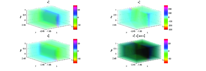
Figure 9: $C_{9}$

IV.10 Critical Point $C_{10}$

For this case, $A^{10}=\left(\begin{array}[]{c}-\frac{\sqrt{6}(1+\omega_{m})}{2\lambda}\\ -\frac{\sqrt{6(1-\omega_{m}^{2})}}{2\lambda}\\ 1\\ \end{array}\right).$

The jacobian matrix of the system (14)-(16) has the characteristic polynomial

$$a^{10}_{3}s^{3}+a^{10}_{2}s^{2}+a^{10}_{1}s+a^{10}_{0}=0$$ (128)

where

$$a^{10}_{3}=1,$$ (129)

$$a^{10}_{2}=\frac{(9\lambda+6\mu+3\lambda\omega_{m}+6\omega_{m}\mu)}{2\lambda},$$ (130)

$$a^{10}_{1}=\frac{9(\omega_{m}^{2}-1)(-2\lambda^{2}-\mu\lambda+3\omega_{m}+3)}{2\lambda^{2}}$$ (131)

and

$$a^{10}_{0}=-\frac{27(\lambda+\mu)(\omega_{m}-1)(\omega_{m}+1)^{2}(-\lambda^{2}+3\omega_{m}+3)}{2\lambda^{3}}.$$ (132)

Then,

$$e^{10}_{1}=\frac{3(\lambda\omega_{m}-\lambda+X9)}{4\lambda},$$ (133)

$$e^{10}_{2}=-\frac{3(\lambda+\mu)(\omega_{m}+1)}{\lambda}$$ (134)

and

$$e^{10}_{3}=\frac{3(\lambda\omega_{m}-\lambda-X9)}{4\lambda}.$$ (135)

$e^{10}_{1}$ and $e^{10}_{3}$ are both zero if $\omega_{m}=1$ or $\omega_{m}=\frac{\lambda^{2}}{3}-1.$ But in the first subcase $C_{10}$ reduces to $C_{9}$ and in the later subcase $C_{10}$ becomes identical with $C_{7}$ or $C_{8}$ depending on whether $\lambda<0$ or $\lambda>0.$ $e^{10}_{2}$ is zero if $\mu=-\lambda.$ Hence $\mu=-\lambda$ is the only interesting subcase.

We present the TABLE 24 containing the non-hyperbolic subcases and their stability.

Table 24: $C_{10}$(Cases)

Case	$\omega_{m}$	$\lambda$	$\mu$
a	$-1<\omega_{m}\leq 1$	$\lambda\neq 0$	$-\lambda$

The center manifolds and the reduced systems are described by the TABLE 25.

Table 25: $C_{10}$(Center Manifolds and Reduced System)

Case	Center Manifold	Reduced System
a	$\bar{\bar{y}}=C^{{10},a}_{1,(2,0,0)}\bar{\bar{x}}^{2},\bar{\bar{\nu}}=C^{{10},a}_{2,(2,0,0)}\bar{\bar{x}}^{2}$	$\bar{\bar{x}}^{\prime}=R^{{10},a}_{1,(4,0,0)}\bar{\bar{x}}^{4}$

where

$$C^{{10},a}_{1,(2,0,0)}=-\frac{\sqrt{6}(1+\omega_{m})^{2}(Y9+Z9X9)}{128\lambda^{2}(1-\omega_{m}^{2})^{\frac{3}{2}}X9},C^{{10},a}_{2,(2,0,0)}=\frac{\sqrt{6}(1+\omega_{m})^{2}(Y9-Z9X9)}{128\lambda^{2}(1-\omega_{m}^{2})^{\frac{3}{2}}X9}$$ (136)

and

$$R^{{10},a}_{1,(4,0,0)}=\frac{18\omega_{m}^{2}-60\omega_{m}+90}{128(1-\omega_{m})^{2}},$$ (137)

where $X9,Y9$ and $Z9$ are as defined for $C_{9}.$

For subcase (a), $P^{10}_{a}=\left(\begin{array}[]{ccc}-\frac{3\sqrt{6}(1+\omega_{m})}{8\lambda}&-M9-N9&M9-N9\\ -\frac{\sqrt{6(1-\omega_{m}^{2})}(3\omega_{m}-1)}{8\lambda(\omega_{m}-1)}&1&1\\ 1&0&0\\ \end{array}\right),$

where $M9$ and $N9$ are as defined in the previous subsection.

In the TABLE 26, we summarize our results for the stability of the reduced system of $C_{10}.$

Table 26: Summary for $C_{10}$(non-hyperbolic scenario)

Case	$\omega_{m}$	$\lambda$	$\mu$	Stability(RS)
a	$-1<\omega_{m}\leq 1$	$\lambda\neq 0$	$-\lambda$	Stable

Lastly we present FIG.10 showing the stability analysis for $C_{10}$ to end our analysis of the critical points. The parameter space considered in FIG.10 is $\{0\leq\omega_{m}\leq 1,-1.65\leq\lambda\leq 1.65,-\sqrt{6}\leq\mu\leq\sqrt{6}\}$.

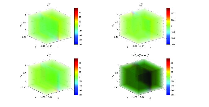
Figure 10: $C_{10}$

We present the phase plane diagrams of the autonomous system (14)-(16) for various values of the parameter $\lambda,\omega_{m}$ and $\mu$’s in FIG. 11 and FIG. 12. We note that, as all the critical points has the $\nu$ component $=1,$ the 2-D phase planes are actually the sections of solutions of (14)-(16) for particular values of $\lambda,\omega_{m},\mu$ at $\nu=1.$

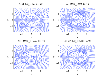
Figure 11: Phase Plane Diagrams (I)

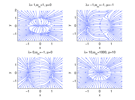
Figure 12: Phase Plane Diagrams (II)

It is to be noted that the quintessence dark energy model with exponential potential can be regarded as a limiting case of the DBI field with exponential potential and warp factor. A nice analytical treatment of autonomus systems for quintessence and other important models of dark energies can be found in CST06 and some interesting applications of the center manifold theory for some of these dark energy models can be found in BCL12 . Indeed, if $f(\phi)\dot{\phi}^{2}<<1,$ then from (5) it is clear that $\nu\approx 1.$ Therefore the field equations of the DBI field $\phi$ described in (1) and the energy density (3) and the pressure density (4), all become identical to those of the quintessence field. Therefore it is no surprise that the critical points related to the quintessence model with the exponential potential, described in the the TABLE I in CST06 should be $\nu\approx 1$ limit of the critical points related to the DBI field, described in the TABLE 1 in this paper. There are five critical points, namely $(a),(b1),(b2),(c)$ and $(d)$ in the TABLE I in CST06 . The critical point $(a)$ is a limiting case of the critical points $C_{9}$ and $C_{10}$ as $\omega_{m}\approx-1.$ The critical points $(b1),(b2)$ and $(c)$ are identical to the $C_{1},C_{2}$ and $C_{7}$ respectively. The critical point $d$ is the $\nu\approx 1$ limit of $C_{9}.$ The critical points $C_{3},C_{4},C_{5},C_{6}$ in our paper only pertain to the DBI field and do not arise in the analysis of the quintessence field. The critical point $(a)$ is ultrarelativistic in nature and $C_{9},C_{10}$ only approaches it as $\omega_{m}\approx-1$, never coincides it. The results of a hyperbolic analysis has been listed in CST06 for all these critical points in the TABLE I. The analysis of the non-hyperbolic cases for the critical point $(b1)$ and $(b2)$ has been done in the TABLES 4 and 6 respectively. In these tables, cases (b) and (d) pertain to the quintessence scenario and provide the result for the non-hyperbolic boundary cases. For the critical pont $(c),$ the center manifold analysis has been done in the TABLE 17. In the TABLE 17, only the case (b) relates to the quintessence situation. From the TABLE 17, it is evident that the stable nature of the non-hyperbolic critical point $C_{7}$ may correspond to the critical pont $(c)$ in CST06 . The non-hyperbolic stability analysis for the critical point $C_{9}$ or it’s $\nu\approx 1$ limit $(d),$ has been done in the TABLE 23. Only the case (b) is applicable for the quintessence case. It is clear that the stable nature of the non-hyperbolic critical point $C_{9}$ corresponds to the critical point (d).

V Cosmological Interpretations and Conclusion

The present work deals with the DBI-cosmology in the framework of dynamical system analysis. Here the DBI scalar field is chosen as the DE while a perfect fluid with barotropic equation of state is chosen as the dark matter. In the section IV we have seen that there are ten critical points $C_{1}-C_{10}.$ They are presented in the TABLE 1. The relevant cosmological parameters at these critical points are given in the TABLE 2. From these tables one may see that the pair of critical points $(C_{1},C_{2}),(C_{3},C_{4}),(C_{5},C_{6}),(C_{7},C_{8})$ and $(C_{9},C_{10})$ are cosmologically equivalent pairwise. We name these pairs as $A,B,C,D$ and $E$ respectively. If one considers the regions $E_{11}=\{\omega_{m}>1,\lambda<-\sqrt{6},\mu<\sqrt{6}\}$ and $E_{12}=\{\omega_{m}<1,\lambda>-\sqrt{6},\mu>\sqrt{6}\},$ then the stability analysis in the interiors of these two regions and in the interior of complement of $E_{11}\cup E_{12}$ is a simple application of the ”Hartman-Gröbman Theorem”. The TABLE 4 in this paper lists the different parts of the boundary between $(E_{11}\cup E_{12})$ and $(E_{11}\cup E_{12})^{c}$ (The superscript ’$c$’ denotes the complement) in case (a)-case (f). With the aid of the Center Manifold Theory, the stability of the system at these parts of the boundaries have been investigated and the results have been listed in the last column of the TABLE 4. From these results, we find that in all the other cases except for the part of the boundary described in case (f)$:=\{\omega_{m}\in\mathbf{R},\lambda=-\sqrt{6},\mu=\sqrt{6}\}$, $C_{1}$ presents a stable solution whereas on the part of the boundary (f) it is unstable. For the cosmologically equivalent critical point $C_{2},$ it turns out that we have similar kind of results. Physically the pair of critical points $A$ represent a DBI scalar field dominated Universe where the scalar field is represented by a perfect fluid having the nature of a stiff fluid and correspond to a decelerating phase of the Universe. So it is not of much interest from the cosmological point of view. As an application of the Hartman-Gröbman Theory, in CSS10 , it has been shown that $C_{3}$ is stable on the region $E_{31}=\{\mu>\sqrt{3(1+\frac{1}{\omega_{m}})},\mu>-\lambda,\lambda<0\}$ and unstable on the region $E_{32}=\{\mu<\sqrt{3(1+\frac{1}{\omega_{m}})},\mu<-\lambda,\lambda<0\}$ and saddle on the interior of $(E_{31}\cup E_{32})^{c}.$ In this paper we have done the stability analysis on the different parts of the boundary between $(E_{31}\cup E_{32})$ and $(E_{31}\cup E_{32})^{c}$ with the aid of Center Manifold Theory. The different parts of the boundary and the stability results on them have been listed on the TABLE 9. These results are entirely new and can not be found in the literature such as  CSS10 . $C_{4}$ has analogus set of results as $C_{3}.$ Physically the set of critical points $B$ are also scalar field dominated and it behaves as dark energy if $\mu^{2}<3$ (i.e. accelerating phase) while for $\mu^{2}>3,$ the DBI scalar field behaves as normal matter with the decelerating era of the Universe. For the critical point $C_{5}$ also, the stability analysis on the parts of the boundary between the open regions, determined by the negativity or the positivity of the eigenvalues has been done by the application of CMT and various stability results such as the stability of the system on the surface $\{\mu=-\lambda,\lambda\neq 0\}$ has been confirmed in this paper. As usual the critical point $C_{6}$ has entirely analogus set of results as $C_{5}$. Physically the pair of critical points $C$ represent scaling solution of the model where both the matter fields have contribution to the evolution. The Universe will be in the accelerating phase if $\omega_{m}<-\frac{1}{3}$ when the scalar field behaves as dark energy. The scaling solution will be dominated by the DE if $\omega_{m}<\frac{6}{\mu^{2}-6}$ otherwise it will be dominated by the dark matter. Similar is the situation for the critical points $E$ with DE dominance if $\omega_{m}>\frac{\lambda^{2}}{6}-1.$ Here for one of the critical points, say $C_{10},$ the parts of the boundary between the open regions in the $\omega_{m}-\lambda-\mu$ space as described above for the other critical points and the stability results on them has been described in the TABLE 17, 20, 23 and 26 with the aid of the CMT. These results are new. $C_{9}$ also has a similar set of results. For $E_{71}=\{\frac{\lambda^{2}}{3}-1<\omega_{m},\lambda>0,\mu>-\lambda\}$ and $E_{72}=\{\frac{\lambda^{2}}{3}-1<\omega_{m},\lambda<0,\mu<-\lambda\}$, according to CSS10 , $C_{7}$ is stable on $(E_{71}\cup E_{72})$. On $(E_{71}\cup E_{72})^{c},$ it is unstable. However the boundary between the regions $(E_{71}\cup E_{72})$ and $(E_{71}\cup E_{72})^{c},$ comprises of the surfaces described in the case (a), (b) and (c) of the TABLE 15 in this paper, (a)$:=\{|\lambda|<\sqrt{6},\lambda\neq 0;\mu=-\lambda,\omega_{m}\in\mathbf{R}\}$, (b)$:=\{|\lambda|<\sqrt{6},\lambda\neq 0;\mu\in\mathbf{R},\omega_{m}=\frac{\lambda^{2}}{3}-1\}$ and (c)$:=\{|\lambda|<\sqrt{6},\lambda\neq 0;\mu=-\lambda,\omega_{m}=\frac{\lambda^{2}}{3}-1\}.$ By the application of CMT, on the surface (a) and (b), $C_{7}$ is stable whereas on the surface (c), $C_{7}$ is unstable. These results tabulated in the TABLE 17 in our paper are entirely new. The stability results of the other critical point $C_{8}$ in the pair $D$ is analogus to $C_{7}.$ Physically the critical points set $D$ is dominated by the DE as the set $B$ with an accelerating phase for $\lambda^{2}<2$ and a decelerating phase for $\lambda^{2}>2.$ Therefore it can be inferred that from the cosmological viewpoint the critical points sets $C$ and $E$ are interesting and one may estimate the parameters $\mu$ and $\lambda$ from the observed results.

VI References

References

- (1) S. J. Perlmutter et al. [Supernova Cosmology Project Collaboration], ”Measurements of Omega and Lambda from 42 high redshift supernovae”, Astrophys. J. 517(2), 565-586 (1999).
- (2) A. J. Reiss et al. [Supernova Search Team], ”Observational evidence from supernovae for an accelerating universe and a cosmological constant”, Astron. J. 116(3), 1009-1038 (1998).
- (3) W. J. Percival et al., ”Measuring the Baryon Acoustic Oscillation scale using the Sloan Digital Sky Survey and 2dF Galaxy Redshift Survey”, Mon. Not. Roy. Astron. Soc. 381(3), 1053-1066 (2007).
- (4) D. N. Spergel et al. [WMAP Collaboration], ”Three Year Wilkinson Microwave Anisotropy Probe (WMAP) Observations: Implications for Cosmology”, Astrophys. J. Suppl. Ser. 170(2), 377-408 (2007).
- (5) E. Komatsu et al. [WMAP Collaboration], ”FIVE-YEAR WILKINSON MICROWAVE ANISOTROPY PROBE OBSERVATIONS: COSMOLOGICAL INTERPRETATION”, Astrophys. J. Suppl. Ser. 180(2), 330-376 (2009).
- (6) S. Weinberg,”The Cosmological Constant Problem”, Rev. Mod. Phys. 61(1), 1-23 (1989).
- (7) L. Amendola, S. Tsujikawa, ”Dark Energy”: Theory. and Observations”, Cambridge, UK: Cambridge University Press (2010).
- (8) S. M. Carroll, Liv. Rev. Lett. 4, 1(2001).
- (9) L. Perko, ”Differential Equations and Dynamical Systems”, Springer-Verlag: New York (1991).
- (10) D. K. Arrowsmith and C. M. Place, ”An Introduction to Dynamical Systems”, Cambridge Univ. Press: Cambridge, England (1990).
- (11) S. Wiggins, ”Introduction to Applied Nonlinear Dynamical Systems and Chaos”, ”2nd Edition”, Springer, Berlin (2003).
- (12) B. Ratra and P. J. E. Peebles, ”Cosmological consequences of a rolling homogeneous scalar field”, Phys. Rev. D 37(12), 3406-3427 (1988).
- (13) R. R. Caldwell and R. Dave and P. J. Steinherdt, ”Cosmological Imprint of an Energy Component with General Equation of State”, Phys. Rev. Lett. 80(8), 1582-1585 (1998).
- (14) C. Armendariz-Picon and V. Mukhanov and P. J. Steinherdt, ”Dynamical Solution to the Problem of a Small Cosmological Constant and Late-Time Cosmic Acceleration”, Phys. Rev. Lett. 85(21), 4438-4441 (2000).
- (15) Amartya S. Banerjee, ”An Introduction to Center Manifold Theory”.
- (16) C. Armendariz-Picon and V. Mukhanov and P. J. Steinherdt, ”Essentials of k-essence”, Phys. Rev. D 63(10), 103510 (2001).
- (17) R. R. Caldwell and M. Kamionkowski and N. N. Weinberg, ”Causes a Cosmic Doomsday”, Phys. Rev. Lett. 91(7), 071301 (2003).
- (18) A. Sen, J. H. E. P 207, 65 (2002).
- (19) E. J. Copeland and A. R. Riddle and D. Wands, ”Exponential potentials and cosmological scaling solutions”, Phys. Rev. D 57(8), 4686-4690 (1998).
- (20) V. Sahni and A. Starobinsky, ”THE CASE FOR A POSITIVE COSMOLOGICAL - TERM”, Int. J. Mod. Phys. D 09(04), 373-443 (2000).
- (21) I. Zlatev and L. Wang and P. J. Steinhardt, ”Quintessence, Cosmic Coincidence, and the Cosmological Constant”, Phys. Rev. Lett. 82(5), 896-899 (1999).
- (22) R. R. Caldwell, ”A phantom menace? Cosmological consequences of a dark energy component with super-negative equation of state”, Phys. Lett. B 545(1-2), 23-29 (2002).
- (23) T. Padmanabhan, ”Accelerated expansion of the Universe driven by tachyonic matter”, Phys. Rev. D 66(2), 021301 (2002).
- (24) F. Piazza and S. Tsujikawa, ”Dilatonic ghost condensate as dark energy”, JCAP 2004(07), 004 (2004).
- (25) E. Elijalde and S. Nojiri and S. D. Odintsov, ”Late-time Cosmology in a (phantom) scalar-tensor theory : Dark energy and the cosmic speed-up”, Phys. Rev. D 70(4), 043539 (2004).
- (26) S. Nojiri and S. D. Odintsov and S. Tsujikawa, ”Properties of singularities in the (phantom) dark energy Universe”, Phys. Rev. D 71(6), 063004 (2005).
- (27) E. Silverstein and D. Tong, ”Scalar speed limits and cosmology : Acceleration from D-eceleration”, Phys. Rev. D 70(10), 103505 (2004).
- (28) X. Chen, ”Multithroat brane inflation”, Phys. Rev. D 71(6), 063506 (2005).
- (29) Luis P. Chimento and Ruth Lazkoz and Martin G. Richarte, ”Enhanced inflation in the Dirac-Born-Infeld framework”, Phys. Rev. D 83(6), 063505 (2011).
- (30) C. Armendariz-Picon and T. Damour and V. Mukhanov, ”K-Inflation”, Phys. Lett. B 458(2-3), 209-218 (1999).
- (31) E. Guendelman and D. Singleton and N. Youngram, ”A two measure model of dark energy and dark matter”, JCAP 2004(07), 004 (2004).
- (32) G. Olivares and F. Atrio-Barandela and D. Pavon, ”Observational constraints on interacting quintessence models”, Phys. Rev. D 71(6), 063523 (2005).
- (33) G. Olivares and F. Atrio-Barandela and D. Pavon, ”Metter density perturbations in interacting quintessence models”, Phys. Rev. D 74(4), 043521 (2006).
- (34) D. Pavon and B. Wang, ”Le Chatelier- Braun principle in cosmological physics”, Gen. Rel. Grav. 41(1), 1-5 (2009).
- (35) C. Kaeonikhom and D. Singleton and S. V. Sushkov and N. Youngram, ”Dynamics of Dirac-Born-Infeld dark energy interacting with dark matter”, Phys. Rev. D 86(12), 124049 (2012).
- (36) N. Mahata and S. Chakraborty, ”Dynamical system Analysis for DBI dark energy interacting with dark matter”, Mod. Phys. Lett. A 30(02), 1550009 (2015).
- (37) E. J. Copeland and M. Shuntaro and M. Shaeri, ”Cosmological dynamics of a Dirac-Born-Infeld field”, Phys. Rev. D 81(12), 123501 (2010).
- (38) M. Hirsch and S. Smale, ”Differential Equations, Dynamical Systems and Linear Algebra”, Academic Press, New York (1974).
- (39) E. J. Copeland and M. Sami and S. Tsujikawa, ”Dynamics of Dark Energy”, Int. J. Mod. Phys. D 15, 1753 (2006).
- (40) C. G. Boehmer and N. Chan and R. Lazkoz, ”Dynamics of dark energy models and centre manifolds”, Phys. Lett. B 714, 11 (2012).