Radion dynamics, heavy Kaluza-Klein resonances and gravitational waves

Abstract

We study the confinement/deconfinement phase transition of the radion field in a warped model with a polynomial bulk potential. The backreaction of the radion on the metric is taken into account by using the superpotential formalism, while the radion effective potential is obtained from a novel formulation which can incorporate the backreaction. The phase transition leads to a stochastic gravitational wave background that depends on the energy scale of the first Kaluza-Klein resonance, $m_{\textrm{\tiny KK}}$. This work completes previous studies in the following aspects: i) we detail the evaluation of the radion spectrum; ii) we report on the mismatches between the thick wall approximation and the numerical bounce solution; iii) we include a suppression factor in the spectrum of sound waves accounting for their finite lifetime; and, iv) we update the bound on $m_{\textrm{\tiny KK}}$ in view of the O3 LIGO and Virgo data. We find that the forthcoming gravitational wave interferometers can probe scenarios where $m_{\textrm{\tiny KK}}\lesssim 10^{9}\,\textrm{TeV}$, while the O3-run bounds rule out warped models with $10^{4}\textrm{TeV}\lesssim m_{\textrm{\tiny KK}}\lesssim 10^{7}\textrm{TeV}$ exhibiting an extremely strong confinement/deconfinement phase transition.

Keywords: Physics beyond the Standard Model, extra dimensions, radion dynamics, electroweak phase transition, gravitational waves.

1 Introduction

The Standard Model (SM) of particle physics is unable to explain experimental observations like the baryon asymmetry of the universe and the existence of dark matter, and suffers from theoretical drawbacks, like the electroweak (EW) hierarchy problem, which is understood as a strong sensitivity to high scale physics. These issues have motivated the study of beyond the SM (BSM) scenarios where new physics is present. In particular, the Randall-Sundrum (RS) model was proposed in 1999 [1] as a way to solve the hierarchy problem between the Planck scale $M_{P}\sim 10^{15}\,\textrm{TeV}$ and the EW scale $\rho\sim\textrm{TeV}$ by means of a warped extra dimension in Anti-de Sitter (AdS) space. This extra dimension determines a spectrum of heavy Kaluza-Klein (KK) resonances, where the mass of the first resonance is $m_{\textrm{\tiny KK}}\sim\rho$. In addition, the model contains a light state, the radion, which is typically the lightest BSM state, with a dynamics dictated by an effective potential.

The LHC data are putting severe lower limits on the masses of the first KK resonances [2, 3]. These limits point toward the possibility that nature might have chosen values of $\rho\gg 1$ TeV. In such a case the EW scale would require some amount of tuning, but the warp factor would still naturally explain the hierarchy between the Planck scale and the value of $\rho$. At the same time the KK excitations would easily escape the LHC searches, and so their discovery would rely on future more energetic colliders.

In the present work we investigate the warped models in the large $\rho>1$ TeV regime. To compute the radion effective potential in the presence of large backreactions, we use a recent development of the so called “superpotential procedure”. In the resulting potential, the radion undergoes a first order phase transition during which it acquires a vacuum expectation value [4, 5, 6]. This phase transition, representing a confinement/deconfinement transition, generates a stochastic gravitational wave background (SGWB) [7] detectable at the present and future gravitational wave interferometers. Thanks to this signature, the warped scenario with KK modes outside the reach of the LHC of future circular colliders, can still be tested.

2 The Randall-Sundrum model

In this section we introduce the main properties of the RS model, and outline the objectives that will be pursued in the rest of the paper. The RS model is based on a 5D space with line element [1]

$$ds^{2}=g_{MN}dx^{M}dx^{N}\equiv e^{-2A(r)}\eta_{\mu\nu}dx^{\mu}dx^{\nu}-dr^{2}\,,\qquad A(r)=kr\,,$$ (1)

and two branes, located at different positions along the coordinate $r$ of the extra dimension. The UV brane, at $r=r_{0}=0$, provides the Planck scale, while the IR brane, at $r=r_{1}$, sets the TeV (or multi-TeV) scale $\rho$. The hierarchy between these scales is driven by the warped space factor

$$\rho=e^{-kr_{1}}M_{P}\qquad\mathrm{with}\qquad kr_{1}\sim 35\,.$$ (2)

Fields that are mainly localized toward the IR brane are composite; this is the case of the Higgs, heavy fermions and KK modes. On the contrary, fields that are localized toward the UV brane are elementary, as e.g. light fermions. Other fields, like the zero mode gauge bosons, have a flat profile in the extra dimension.

In the RS model the brane distance has to be stabilized. This can be achieved by a bulk scalar field $\phi$ that softly breaks conformal invariance and has some bulk and brane potentials fixing its vacuum expectation value [8]. Due to this gentle breaking, the degree of freedom regulating the brane distance tends to yield a light state. The corresponding field, dubbed as radion or dilaton depending on the (5D or 4D) context, is coupled to the SM and exhibits an interesting Higgs-like phenomenology [9]. Nevertheless, the RS model has problems when confronting to EW precision measurements. In particular, it fails to describe oblique observables $S,T,U$, as it leads to too large values of them. Several ideas have been proposed to circumvent the issue:

• Considering a large backreaction on the metric such as to create a singularity. This is achieved by using a deformed metric in the IR [10, 11].

• Assuming custodial symmetry in the bulk conserved in the IR [12].

• Moving the KK resonance masses above the TeV scale, e.g. $m_{\textrm{\tiny KK}}\gtrsim 10$ TeV [13].

In this paper we explore the third possibility. It has several implications, in particular the model stops aiming for being a fully naturally solution of the “whole” hierarchy problem – a little hierarchy problem remains –, although it still substantially relaxes it. Moreover this is what the collider data may be hinting at, with no observation of stable narrow resonances close to the TeV scale. Nevertheless, this heavy-KK scenario remains testable. As we will discuss hereafter, the present and future gravitational wave interferometers can indirectly probe KK resonances heavier than the TeV scale.

3 The radion effective potential

In this section we review for completeness details on the radion effective potential and the formalism we adopt [13].

3.1 General formalism

We consider the 5D action of the model [13]

$$S = \int d^{5}x\sqrt{|\det g_{MN}|}\left[-\frac{1}{2\kappa^{2}}R+\frac{1}{2}g^{MN}(\partial_{M}\phi)(\partial_{N}\phi)-V(\phi)\right]$$ (3)

$$-\sum_{\alpha}\int_{B_{\alpha}}d^{4}x\sqrt{|\det\bar{g}_{\mu\nu}|}\Lambda_{\alpha}(\phi)+S_{\rm GHY}\,,$$

where $S_{\rm GHY}$ is the standard Gibbons-Hawking-York boundary term, $V(\phi)$ is the bulk scalar potential, $\Lambda_{\alpha}(\phi)$ are the UV $(\alpha=0)$ and IR $(\alpha=1)$ 4D brane potentials located at $\phi_{\alpha}\equiv\phi(r_{\alpha})$, and $\kappa^{2}=1/(2M_{5}^{3})$ with $M_{5}$ being the 5D Planck scale. The metric is defined as in Eq. (1) where the 4D induced metric is $\bar{g}_{\mu\nu}=e^{-2A(y)}\eta_{\mu\nu}$, and the Minkowski metric is given by $\eta_{\mu\nu}=\textrm{diag}(1,-1,-1,-1)$. To solve the hierarchy problem, the brane dynamics must lead to values of $\phi_{0}$ and $\phi_{1}$ yielding $A(\phi_{1})-A(\phi_{0})\approx\log(M_{P}/\rho)$, in analogy with Eq. (2).

The classical equations of motion (EoM) in the bulk can be expressed in terms of the superpotential $W(\phi)$ as

$$\phi^{\prime}(r)=\frac{1}{2}W^{\prime}(\phi)\,,\qquad A^{\prime}(r)=\frac{\kappa^{2}}{6}W(\phi)\,,\qquad V(\phi)=\frac{1}{8}\left[W^{\prime}(\phi)\right]^{2}-\frac{\kappa^{2}}{6}W^{2}(\phi)\,.$$ (4)

For the brane potentials we consider $\Lambda_{\alpha}(\phi)=\Lambda_{\alpha}+\frac{1}{2}\gamma_{\alpha}(\phi-v_{\alpha})^{2}$, following the Goldberger-Wise mechanism [14] to fix the values of the scalar field at the branes equal to $v_{\alpha}$. As in Ref. [14], we work in the stiff potentials limit, where $\gamma_{\alpha}\to\infty$, such that $\phi(r_{\alpha})=v_{\alpha}$. We use the freedom on $A(r_{0})$ to set $A(r_{0})=0$. Consequently, the relationship between the 5D and 4D Planck masses is fixed via the expression

$$\kappa^{2}M_{P}^{2}=2\ell\int_{0}^{\bar{r}_{1}}d\bar{r}\,e^{-2A(\bar{r})}\,,$$ (5)

where $\ell$ is the radius of AdS, while $\bar{r}\equiv r/\ell$ and $M_{P}=2.4\times 10^{18}\,\textrm{GeV}$.

3.2 The effective potential in the warped model

Using the EoM, one can express the on-shell action of the model as the 4D integral $S=-\int d^{4}x\,U_{\textrm{\scriptsize eff}}$ where the effective potential $U_{\textrm{\scriptsize eff}}$ is

$$U_{\textrm{\scriptsize eff}}=\left[e^{-4A}\left(W+\Lambda_{1}\right)\right]_{r_{1}}+\left[e^{-4A}\left(-W+\Lambda_{0}\right)\right]_{r_{0}}\,.$$ (6)

We now introduce a novel technique to compute $U_{\textrm{\scriptsize eff}}$. Firstly, notice that the EoM for $W$ with potential $V$, cf. Eq. (4), is a first order differential equation, so that it admits an integration constant that we denote by $s$. If $W_{0}$ is a particular solution of the EoM, then it is possible to find a general solution of the equation as an expansion of the form [15, 16, 17]

$$W=\sum_{n=0}^{\infty}s^{n}W_{n}\,,$$ (7)

where $W_{n}$ can be computed iteratively from $W_{0}$. An explicit solution for $n=1$ is given by

$$W_{1}(\phi)=\frac{1}{\ell\kappa^{2}}\exp\left(\frac{4\kappa^{2}}{3}\int^{\phi}\frac{W_{0}(\tilde{\phi})}{W^{\prime}_{0}(\tilde{\phi})}d\tilde{\phi}\right)\,.$$ (8)

We can similarly expand the scalar field $\phi$ and the warp factor $A$ as

$$\phi(r)=\phi_{0}(r)+s\,\phi_{1}(r)+\mathcal{O}(s^{2})\,,\qquad A(r)=A_{0}(r)+s\,A_{1}(r)+\mathcal{O}(s^{2})\,.$$ (9)

The integration constant $s$ is fixed by the boundary condition $\phi(r_{1})=v_{1}$ leading to

$$s(r_{1})=\frac{v_{1}-\phi_{0}(r_{1})}{\phi_{1}[\phi_{0}(r_{1})]}\,.$$ (10)

Therefore, the superpotential acquires an explicit dependence on the brane distance $r_{1}$, i.e.

$$W(v_{\alpha})=W_{0}(v_{\alpha})+s(r_{1})W_{1}(v_{\alpha})+\cdots\,,\qquad\textrm{with}\qquad\alpha=0,1\,,$$ (11)

which in turn creates a non-trivial dependence on $r_{1}$ of the effective potential of Eq. (6). Finally, the effective potential normalized to its value at $r_{1}\to\infty$ is given by

$$U_{\textrm{\scriptsize eff}}(r_{1})=[\Lambda_{1}+W_{0}(v_{1})]e^{-4A_{0}(r_{1})}[1-4A_{1}(r_{1})s(r_{1})]+s(r_{1})\left[e^{-4A_{0}(r_{1})}W_{1}(v_{1})-W_{1}(v_{0})\right]$$ (12)

where $\Lambda_{1}$ is the tension at the IR brane. In this expression we have retained terms up to first order in $s(r_{1})$, an expansion which has been proven a posteriori to be valid.

The next step is to apply this technique to the warped phenomenological model given by

$$W_{0}(\phi)=\frac{6}{\ell\kappa^{2}}+\frac{u}{\ell}\phi^{2}\,,$$ (13)

with $\ell\sim{\mathcal{O}}(M_{5}^{-1})$. In this scenario, the scalar field and warp factor turn out to be

$$\bar{\phi}_{0}(r)=\bar{v}_{0}\,e^{u\bar{r}}\,,\qquad A_{0}(r)=\bar{r}+\frac{\bar{v}_{0}^{2}}{12}\left(e^{2u\bar{r}}-1\right)\,,$$ (14)

where we have defined the dimensionless quantities $\bar{\phi}\equiv\kappa\phi$ and $\bar{v}_{a}\equiv\kappa v_{a}$. A solution of the EoM is also $W(\phi)=W_{0}(\phi)+sW_{1}(\phi)+\cdots$, with

$$W_{1}(\phi)=\frac{1}{\ell\kappa^{2}}\left(\frac{\phi}{v_{0}}\right)^{4/u}e^{\kappa^{2}(\phi^{2}-v_{0}^{2})/3}\,.$$ (15)

This leads to ${\mathcal{O}}(s)$ corrections in $\phi(r)$ and $A(r)$ via the EoM of Eq. (4).

Let us first consider the simple case in which we tune to zero the first term of Eq. (12), namely we choose $\Lambda_{1}=-W_{0}(v_{1})$. Then, by defining the dimensionless effective potential $\bar{U}_{\textrm{\scriptsize eff}}(r_{1})\equiv\ell\kappa^{2}U_{\textrm{\scriptsize eff}}(r_{1})$, we find

$$\bar{U}_{\textrm{\scriptsize eff}}^{0}(\bar{r}_{1})=2u^{2}\bar{v}_{1}^{2}(\bar{r}_{1}^{0}-\bar{r}_{1})\left[e^{4A_{0}(\bar{r}_{1}^{0})-4A_{0}(\bar{r}_{1})}-1\right]\,e^{-4A_{0}(\bar{r}_{1})}\,,$$ (16)

with $v_{1}\equiv v_{0}\,e^{u\bar{r}_{1}^{0}}$. This effective potential is positive definite, and it vanishes when $u=0$, i.e. in the absence of backreaction. In the left panel of Fig. 1 we display the tuned effective potential of Eq. (16) as well as, for the sake of comparison, the Goldberger-Wise potential of Ref. [14], denoted by $\bar{U}_{\textrm{\scriptsize eff}}^{0\;\rm GW}$. The agreement turns out to be much better when considering $\bar{U}_{\textrm{\scriptsize eff}}^{0}$ with an artificially neglected backreaction on the metric, $\bar{U}_{\textrm{\scriptsize eff}}^{0\rm NB}$, i.e. using $A_{0}(r)\simeq\bar{r}$. Notice that $\bar{U}_{\textrm{\scriptsize eff}}^{0\;\rm GW}$ and $\bar{U}_{\textrm{\scriptsize eff}}^{0\;\rm NB}$ have been computed using completely different methods.

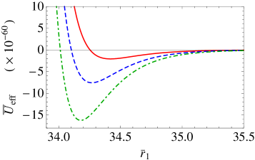
Figure 1: Left panel: The potential $\bar{U}_{\textrm{\scriptsize eff}}^{0}$ in Eq. (16) (solid line), the same potential when neglecting the backreaction $\bar{U}_{\textrm{\scriptsize eff}}^{0\rm NB}$ (dashed line), and the Goldberger-Wise potential $\bar{U}_{\textrm{\scriptsize eff}}^{0\rm GW}$ of Ref. [14] (dashed-dotted line) as functions of $\bar{r}_{1}$. Right panel: The potential $\bar{U}_{\textrm{\scriptsize eff}}$ in Eq. (17) for $\lambda_{1}=-1$ (red solid line), $\lambda_{1}=-2$ (blue dashed line) and $\lambda_{1}=-3$ (green dashed-dotted line). In both panels we assume $\bar{v}_{0}=1,\,\bar{v}_{1}=2,\,u=0.0192$ .

The tuned potential has degenerate minima at $\bar{r}_{1}=\bar{r}_{1}^{0}$ and $\bar{r}_{1}=+\infty$, a fact that prevents a confinement/deconfinement phase transition in an expanding universe. However, this transition is allowed in the detuned potential, which is obtained when using the condition $\Lambda_{1}+W_{0}(v_{1})\equiv\frac{6}{\ell\kappa^{2}}\lambda_{1}\neq 0$, where $\lambda_{1}$ is a dimensionless parameter. The detuned effective potential is given by

$$\bar{U}_{\textrm{\scriptsize eff}}(\bar{r}_{1})\simeq\bar{U}^{0}_{\textrm{\scriptsize eff}}(\bar{r}_{1})+6\lambda_{1}e^{-4A_{0}(\bar{r}_{1})}\,,$$ (17)

which has a minimum located at

$$\bar{r}_{1}^{\textrm{\scriptsize m}}=\bar{r}_{1}^{0}-\frac{1}{4}\mathcal{W}\left[-\frac{6\lambda_{1}}{u^{2}\bar{v}_{1}^{2}}\right]\,,$$ (18)

where $\mathcal{W}(z)$ is the Lambert function. In the right panel of Fig. 1 we plot the effective potential in Eq. (17) for various values of $\lambda_{1}$. Notice that for $\lambda_{1}<0$ the global minimum is at $\bar{r}_{1}^{\textrm{\scriptsize m}}<\bar{r}_{1}^{0}$.

3.3 The radion field

The radion field is obtained by considering a scalar perturbation of the metric, i.e. $ds^{2}=e^{-2A(r)-2F(x,y)}\eta_{\mu\nu}dx^{\mu}dx^{\nu}-[1+2F(x,r)]^{2}dr^{2}$ with $F(x,r)=F(r)\mathcal{R}(x)$. The Lagrangian for the canonically normalized radion field $\chi(r)$ writes as

$$\mathcal{L}_{\textrm{\scriptsize rad}}=\frac{6\ell^{3}}{\kappa^{2}}\int d^{4}x\sqrt{|\det\bar{g}_{\mu\nu}|}\bigg{(}\frac{1}{2}(\partial_{\mu}\chi)^{2}-V_{\rm rad}(\chi)\bigg{)}\,,$$ (19)

where $V_{\textrm{\scriptsize rad}}(\chi)\equiv U_{\textrm{\scriptsize eff}}[\bar{r}_{1}(\chi)]\simeq\frac{1}{2}m_{\textrm{\scriptsize rad}}^{2}\,\chi^{2}$. To leading approximation in the parameter $u$, one finds

$$\chi(r_{1})\simeq\frac{1}{\ell}e^{-A_{0}(r_{1})}\,.$$ (20)

The radion potential has a minimum at $\langle\chi\rangle=\rho$, with $\rho\equiv\frac{1}{\ell}e^{-A_{0}(\bar{r}_{1}^{m})}$. The energy scale set by $\rho$ is the physically relevant parameter that is usually considered at the TeV scale. $\rho$ is mainly determined by $u$, so that for instance we find $u\simeq 0.0192\,(0.0219)$ for $\rho=1\,(100)$ TeV.

The radion mass can be computed by solving the EoM of the scalar perturbation. Using the background EoM one can recast the bulk EoM and boundary conditions for the excitation $F$ as [18]

$$\partial_{r}\left(e^{2A}A^{\prime\prime}(r)^{-1}\partial_{r}\left[e^{-2A}F\right]\right)+\left(m_{\rm rad}^{2}e^{2A}A^{\prime\prime}(r)^{-1}-2\right)F=0\,,$$ (21)

$$\hskip 108.12054pt\left[m_{\rm rad}^{2}F+U_{\alpha}^{\prime\prime}[\phi(r)]\partial_{r}[e^{-2A}F]\right]\Big{|}_{r_{\alpha}}=0\,,$$ (22)

where the localized effective potentials are defined by $U_{\alpha}(\phi)=\Lambda_{\alpha}(\phi)-(-1)^{\alpha}W(\phi)$. The solution of the EoM can be computed, either numerically or by using some analytical mass formulas obtained in the light radion approximation (see e.g. Ref. [11]). In the stiff limit of the brane potentials, for which the radion mass is maximized, the mass formula reads

$$\frac{m_{\rm rad}^{2}}{\rho^{2}}=\frac{1}{\Pi_{\rm rad}}\,,$$ (23)

with

$$\Pi_{\rm rad} = \frac{1}{\ell^{2}}\int_{0}^{r_{1}^{\textrm{\tiny m}}}dre^{4(r-r_{1}^{\textrm{\tiny m}})/\ell}e^{4[\Delta A(r)-\Delta A(r_{1}^{\textrm{\tiny m}})]}\left(\frac{W[\phi(r)]}{W^{\prime}[\phi(r)]}\right)^{2}$$ (24)

$$\qquad\times\left[\frac{2}{W[\phi(r_{1}^{\textrm{\tiny m}})]}+\int_{r}^{r_{1}^{\textrm{\tiny m}}}d\bar{r}e^{-2[A(\bar{r})-A(r_{1}^{\textrm{\tiny m}})]}\left(\frac{W^{\prime}[\phi(\bar{r})]}{W[\phi(\bar{r})]}\right)^{2}\right]\,,$$

where $\Delta A(r)\equiv A(r)-\bar{r}$. The integral in Eq. (24) is dominated by the region $r\simeq r_{1}^{\textrm{\scriptsize m}}$. Its analytical approximation in the limit of $u\ll 1$ is given by 

$$\Pi_{\rm rad}\simeq\frac{1}{4\ell}\frac{2}{W[\phi(r_{1}^{m})]}\,f(\bar{r}_{1}^{m}-1/4)\,,\\$$

and therefore

$$\frac{m_{\rm rad}}{\rho}\simeq\left.e^{2[\Delta A(\bar{r}_{1}^{m})-\Delta A(r)]}\sqrt{2\ell\,W[\phi(r_{1}^{m})]}\,\frac{W^{\prime}[\phi(r)]}{W[\phi(r)]}\right|_{\bar{r}=\bar{r}_{1}^{m}-1/4}\,.$$ (25)

The results using the numerical calculation and this mass formula are displayed in Fig. 2. Both results are in reasonable agreement: for $\bar{v}_{0}=1$, $\bar{v}_{1}=2$ and $\rho=1\textrm{ and }100\,\textrm{TeV}$, the radion mass is $m_{\rm rad}/\rho\simeq 0.10$, and it scales linearly with the values of $\bar{v}_{0,1}$, while it is almost independent of $\lambda_{1}$.

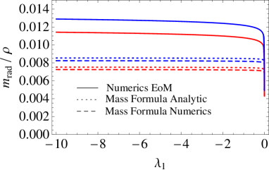
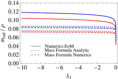
Figure 2: The normalized radion mass $m_{\rm rad}/\rho$ as a function of $\lambda_{1}$ for $\bar{v}_{0}=0.1$ and $\bar{v}_{1}=0.2$ (left panel) and for $\bar{v}_{0}=1$ and $\bar{v}_{1}=2$ (right panel). The red and blue lines are obtained for $\rho=1$ TeV and $\rho=100$  TeV, respectively. The solid lines are evaluated by means of the exact numerical solution of the radion EoM, Eqs. (21)-(22). The results by using the mass formulas have been evaluated in two ways: i) fully numerically as it is written in Eqs. (23)-(24) (dashed lines), and ii) using the analytical approximation given by Eq. (25) (dotted lines).

Using similar approaches, we can compute the mass of the first KK resonance for gauge bosons and gravitons, and we obtain $m_{\rm KK}^{\rm gauge}/\rho\simeq 2.46$ and $m_{\rm KK}^{\rm grav}/\rho\simeq 3.88$, values almost independent of $\bar{v}_{0,1}$, $\lambda_{1}$ and $\rho$. Then, we find a hierarchy of scales $m_{\textrm{\scriptsize rad}}\ll m_{\textrm{\tiny KK}}^{\rm gauge}\lesssim m_{\textrm{\tiny KK}}^{\rm grav}$, which guarantees that the theory is perturbative.

4 The phase transition

In the AdS/CFT correspondence a black hole (BH) solution describes the high temperature phase of the theory. In this phase the dilaton is in the symmetric phase $\langle\chi\rangle=0$. The BH metric is

$$ds_{\textrm{\scriptsize BH}}^{2}=-h(r)^{-1}dr^{2}+e^{-2A(r)}(h(r)dt^{2}-d\vec{x}^{\,2})\,,$$ (26)

where the blackening factor $h(r)$ vanishes at the event horizon, i.e. $h(r_{h})=0$, and satisfies the boundary condition $h(0)=1$. The solution of the EoM in the $u\ll 1$ limit leads to

$$h(r)\simeq 1-e^{4[A_{0}(r)-A_{0}(r_{h})]}\,.$$ (27)

Then, the Hawking temperature and the minimum of the free energy in the BH solution read as

$$T_{h}=\frac{1}{4\pi}e^{-A(r_{h})}\big{|}h^{\prime}(r)\big{|}_{r=r_{h}}\simeq\frac{1}{\ell\pi}e^{-A_{0}(r_{h})}\,,\qquad F_{\min}^{\textrm{\scriptsize BH}}(T)\simeq-\frac{\pi^{4}\ell^{3}}{\kappa^{2}}T^{4}\,.$$ (28)

Below a given temperature, a competing phase with $\langle\chi\rangle\neq 0$ arises. This is the confined phase. The free energies of the BH deconfined phase and the confined phase are

$$F_{d}(T)=E_{0}+F_{\min}^{\textrm{\scriptsize BH}}-\frac{\pi^{2}}{90}g_{d}^{\textrm{\scriptsize eff}}T^{4}\,,\qquad F_{c}(T)=-\frac{\pi^{2}}{90}g_{c}^{\textrm{\scriptsize eff}}T^{4}\,,$$ (29)

where $E_{0}=V_{\textrm{\scriptsize rad}}(0)-V_{\textrm{\scriptsize rad}}(\rho)>0$ is the $T=0$ potential gap between the two phases. For concreteness we assume $g_{c}^{\textrm{\scriptsize eff}}\simeq g_{d}^{\textrm{\scriptsize eff}}\simeq 100$. The phase transition can start when $F_{d}\leq F_{c}$, so that we can define the critical temperature as $F_{d}(T_{c})=F_{c}(T_{c})$. Since the two phases are separated by a potential barrier, the phase transition proceeds through bubble nucleation of the confined phase in the deconfined sea. It happens when the barrier between the false BH minimum and the true vacuum is overcome with sufficiently high probability. While at high $T$ this process is driven by thermal fluctuations and the corresponding Euclidean action is $O(3)$ symmetric, at low $T$ the transition happens via quantum fluctuations with an $O(4)$ symmetric action.

The Euclidean action with symmetry $O(n)$ is given by

$$S_{n}=\Omega_{n}\int d\sigma\sigma^{n-1}\frac{6\ell^{3}}{\kappa^{2}}\left(\frac{1}{2}\left(\frac{\partial\chi}{\partial\sigma}\right)^{2}+V(\chi,T)\right)\,,$$ (30)

with

$$V(\chi,T)\equiv\frac{\kappa^{2}}{6\ell^{3}}\left(V_{\textrm{\scriptsize rad}}(\chi)+\left|F_{\min}^{\textrm{\scriptsize BH}}(T)\right|\right)\,.$$ (31)

The quantity $\Omega_{n}=n\pi^{n/2}/\Gamma(1+n/2)$ is the surface of the unit $n$-sphere, and we define $\sigma=\sqrt{\vec{x}^{2}}$ and $\sigma=\sqrt{\vec{x}^{2}+\tau^{2}}$ for $n=3$ and $n=4$, respectively. Here $\tau$ is the Euclidean time. The corresponding EoM is known as the “bounce equation”, and it is written as [19, 20]

$$\frac{\partial^{2}\chi}{\partial\sigma^{2}}+\frac{(n-1)}{\sigma}\frac{\partial\chi}{\partial\sigma}-\frac{\partial V}{\partial\chi}=0\,,$$ (32)

with boundary conditions $\chi(0)=\chi_{0}$ and $d\chi/d\sigma\big{|}_{\sigma=0}=0$. The corresponding temperature is obtained by equating the kinetic energy of the radion at the origin, $\chi=0$, with the thermal energy, so that the barrier between the two vacua can be overcome, i.e.

$$\frac{3\ell^{3}}{\kappa^{2}}\left(\frac{\partial\chi}{\partial\sigma}\right)^{2}\Bigg{|}_{\chi=0}=\left|F_{\min}^{\textrm{\scriptsize BH}}(T)\right|\,.$$ (33)

The bubble nucleation rate from the false BH minimum to the true vacuum per Hubble volume $\mathcal{V}$ is $\Gamma/\mathcal{V}\sim T_{c}^{4}\left(e^{-S_{3}/T}+e^{-S_{4}}\right)$, so that it is dominated by the least action. The onset of the transition occurs at the nucleation temperature $T_{n}$, with $T_{n}<T_{c}$, defined as the temperature at which the probability for a single bubble to be nucleated within one horizon volume is $\mathcal{O}(1)$. This corresponds to [21]

$$S_{E}(T_{n})\lesssim 4\log\frac{M_{P}/\rho}{T_{n}/\rho}\;\approx\left\{\begin{array}[]{cc}140&\qquad\textrm{for}\qquad\rho\approx 1\,\textrm{TeV}\\ 120&\qquad\quad\textrm{for}\qquad\rho\approx 100\,\textrm{TeV}\end{array}\,.\right.$$ (34)

In the regime where bubble formation is dominated by thick wall bubbles [5], one may consider the thick wall approximations [22]:

$$\frac{S_{3}(T)}{T}\simeq\frac{\sqrt{3}N^{2}}{(\pi T/\rho)\sqrt{{\mathcal{V}}(T/\rho)}}\,,\qquad S_{4}(T)\simeq\frac{9N^{2}}{4{\mathcal{V}}(T/\rho)}\,,$$ (35)

where $N$ is the number of colors in the dual CFT theory, and $\mathcal{V}(T/\rho)=\pi^{4}(T_{c}^{4}-T^{4})/\rho^{4}$. By means of the AdS/CFT duality, $N$ is connected to the 5D squared gravitational coupling constant $(M_{5}\ell)^{-3}$ via the relationship $N^{2}=(M_{5}\ell)^{3}16\pi^{2}$, so that the gravitational theory is weakly coupled in the limit $N\gg 1$. However, from expressions (35) we see that in the limit $N\to\infty$ the actions diverge and there is no phase transition at all. At finite $N$, instead, the phase transition occurs and the tunneling temperature depends on the value of $N$ (see next section). Although the formulas of Eq. (35) are quite intuitive, we find that the thick wall approximation often mismatches the fully numerical result. The nucleation temperatures calculated with one or the other method can differ by almost an order of magnitude. We do not investigate further the reason, as computing $S_{3}/T$ and $S_{4}$ by solving numerically the bounce equation (32) is not very demanding. We mostly comment on this aspect to rise awareness on the issue.

In Fig. 3 we display the Euclidean actions as functions of the temperature computed numerically. In the left panel we present a scenario where the phase transition is dominated by the ${\mathcal{O}}(3)$ contribution, while in the left panel by the ${\mathcal{O}}(4)$ contribution. The curves are normalized by the number of colors in the dual theory.

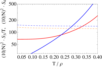
Figure 3: The Euclidean actions $S_{3}/T$ (red) and $S_{4}$ (blue) as functions of $T$ computed by solving numerically the bounce equation (32). We display the cases of $\lambda_{1}=-3.0$ (left panel) and $\lambda_{1}=-5.0$ (right panel). Horizontal blue (orange) lines correspond to the bounds for $\rho=1$ TeV (100 TeV), cf. Eq. (34).

It is useful to notice that a short inflationary epoch precedes the phase transition, and some reheating is realized after it. Inflation starts at the temperature $T_{i}$ such that $E_{0}$ dominates the value of energy density in the deconfined phase, $\rho_{d}$, over the thermal corrections, where

$$\rho_{d}(T)=E_{0}+\frac{3\pi^{4}\ell^{3}}{\kappa^{2}}T^{4}+\frac{\pi^{2}}{30}g_{d}^{\textrm{\scriptsize eff}}T^{4}\,.$$ (36)

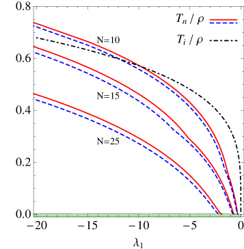
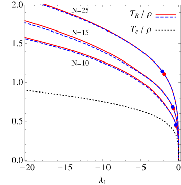
Figure 4: The normalized temperatures $T_{n}/\rho$ (left panel, solid and dashed curves), $T_{i}/\rho$ (left panel, dashed-dotted black curve), $T_{R}/\rho$ (right panel, solid and dashed curves) and $T_{c}/\rho$ (right panel, dotted black curve) as a function of $\lambda_{1}$ for different values of $N$ and $\rho$. Solid-red and dashed-blue lines correspond to the scenarios with $\rho=1$ TeV and $\rho=100$ TeV, respectively.

After the phase transition, $\rho_{d}$ is converted into radiation density in the confined phase. The temperature then goes up to the reheat temperature $T_{R}$, which is obtained from the requirement $\rho_{c}(T_{R})=\pi^{2}g_{c}^{\textrm{\scriptsize eff}}T_{R}^{4}/30\simeq\rho_{d}(T_{n})$. The gravitational radiation is a subleading contribution. Fig. 4 shows the behavior of $T_{n}$ and $T_{i}$ (left panel) as well as $T_{R}$ and $T_{c}$ (right panel) as functions of $\lambda_{1}$ for different values of $N$ and $\rho$. As expected, the condition $T_{R}>T_{c}$ is always satisfied. The big bang nucleosynthesis (BBN) bound excludes the shadowed (green) region on the bottom of the left panel as $T_{n}/\rho\gtrsim 3\times 10^{-4}\sqrt{N}$ [13]. The circles in the right panel correspond to lower bounds of parameter configurations on the border of the BBN bound.

5 The stochastic gravitational waves background

A cosmological first order phase transition generates a SGWB with a power spectrum $\Omega_{\textrm{\scriptsize GW}}(f)$ depending on the dynamics of the bubbles in the plasma. Here we consider two different approaches to estimate $\Omega_{\textrm{\scriptsize GW}}(f)$: the envelope approximation, $\Omega^{\textrm{\scriptsize env}}_{\textrm{\scriptsize GW}}(f)$, in which plasma effects are assumed to be negligible [7, 23], and the sound waves numerical result, $\Omega^{\textrm{\scriptsize sw}}_{\textrm{\scriptsize GW}}(f)$, in which the coherent motion of the plasma is taken into account [7, 24, 25]. The power spectra in these two regimes can be approximated as

$$\Omega^{\textrm{\scriptsize env}}_{\textrm{\scriptsize GW}}(f)\simeq\frac{3.8\,x^{2.8}}{1+2.8\,x^{3.8}}\,\overline{\Omega}_{\rm GW}^{\,\textrm{\scriptsize env}}\,,\qquad\Omega^{\textrm{\scriptsize sw}}_{\textrm{\scriptsize GW}}(f)\simeq x^{3}\left(\frac{7}{4+3\,x^{2}}\right)^{7/2}\,\overline{\Omega}_{\rm GW}^{\,\rm sw}\,,$$ (37)

where $f_{p}$ is the peak frequency, $\overline{\Omega}_{\rm GW}^{\,\textrm{\scriptsize env}(\textrm{\scriptsize sw})}$ is the corresponding amplitude at the peak, and $x=f/f_{p}$. The quantities $f_{p}$ and $\overline{\Omega}_{\rm GW}^{\,\textrm{\scriptsize env}(\textrm{\scriptsize sw})}$ depend on the phase transition parameters $v_{w}$, $\alpha$ and $\beta/H_{\star}$, which are respectively the bubble expansion velocity, the normalized gap between the energies in the two phases, and the inverse time duration of the phase transition. The explicit dependence of $\overline{\Omega}_{\rm GW}^{\,\textrm{\scriptsize sw}}$ and $\overline{\Omega}_{\rm GW}^{\,\textrm{\scriptsize env}}$ are taken from Refs. [7, 25], although in the former we have introduced an additional suppression factor accounting for the sound wave finite lifetime effect [26, 27]. Its order of magnitude is inferred from Fig. 17 of Ref. [28] although, in the lack of simulations at $\alpha\gg 1$, it should be considered only as a rough estimator of the possible uncertainties affecting the SGWB prediction.

For the bubble expansion velocity, there is no unquestionable way to calculate it in the case of the radion transition, hence we treat it as an external input and set it at $0.8\lesssim v_{w}\lesssim 1$ (in the scale of our plots, the variation of $v_{w}$ within this interval is not visible). The energy gap and the inverse time duration can instead be approximated as [7, 25]

$$\alpha\simeq\frac{|F_{d}(T_{n})-F_{c}(T_{n})|}{\rho_{d}^{\ast}(T_{n})}\;\qquad,\qquad\frac{\beta}{H_{\star}}\simeq T_{n}\frac{dS_{E}}{dT}\bigg{|}_{T=T_{n}}\,,$$ (38)

where $\rho_{d}^{\ast}(T_{n})=\rho_{d}(T_{n})-E_{0}$. The larger $\alpha$ and smaller $\beta/H_{\star}$, the stronger the SGWB signal.

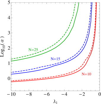
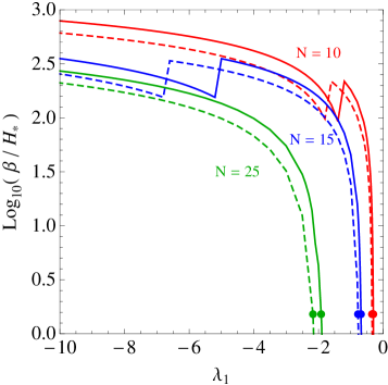
Figure 5: The parameters $\alpha$ (left panel) and $\beta/H_{\star}$ (right panel) as functions of $\lambda_{1}$ for different values of $N$ and $\rho$. Solid and dashed lines assume $\rho=1$ TeV and $\rho=100$ TeV, respectively.

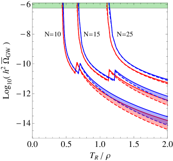
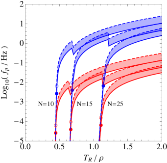
Figure 6: The normalized maximal amplitude $h^{2}\overline{\Omega}_{\textrm{\tiny GW}}$ (left panel) and its frequency $f_{p}$ (right panel) as a function of $T_{R}/\rho$ for different values of $N$ and $\rho$. The strips are for $\rho=1$ TeV (red) and $\rho=100$ TeV (blue). The shadowed green region in the left panel is excluded by BBN. In the right panel, the border of the BBN bound corresponds to the circles. We have considered for the wall velocity $v_{\omega}\simeq 0.99$.

In Fig. 5 we show the curves of $\alpha$ (left panel) and $\beta/H_{\star}$ (right panel) as functions of $\lambda_{1}$, for some values of $N$ and $\rho$. The value of $h^{2}\overline{\Omega}_{\textrm{\scriptsize GW}}^{\textrm{\scriptsize env}(\textrm{\scriptsize sw})}$ and $f_{p}$ obtained along these curves are presented in Fig. 6. Here $h\simeq 0.67$ is the scaling factor for the Hubble parameter and is introduced to keep the result independent of the precise value of today’s Hubble parameter. In Fig. 7 we display the detectability prospects to the parameter space $\{h^{2}\overline{\Omega}_{\textrm{\scriptsize GW}},f_{p}\}$. Within each detector region, the SGWB sourced by a first-order phase transition following the envelope (regions inside the dotted borders) and sound wave (regions inside the dashed borders) behavior, is detected with signal-to-noise ratio SNR$\,\geq 2$ (upper panels) and SNR$\,\geq 1000$ (lower panels). The SNR is calculated as

$${\rm SNR}=\sqrt{(3.16\times 10^{7}s)\frac{\mathcal{T}}{\textrm{1 year}}\int_{0}^{\infty}df\frac{\Omega_{\rm GW}^{2}(f)}{\Omega_{\rm sens}^{2}(f)}}~{},$$ (39)

where $\Omega_{\rm sens}(f)$ is the sensitivity curve of the experiment and $\mathcal{T}$ is the total time (in years) during which a given experiment takes data. For concreteness, we have used 3 years for LISA, 7 years for ET, and 8 years for aLIGO design. The parameter region labeled BBN and aLIGO O3 are in tension with data [13, 29] . The fact that in the lower panels the aLIGO design detection region falls inside the LIGO O3 exclusion region indicates that no first order phase transition with SNR larger than 1000 will be ever observed with the aLIGO design sensitivity since such a powerful signal is already ruled out.

In Fig. 7 the diagonal strips correspond to the predictions in our warped setup for $\rho=1\textrm{ TeV}$ (left panels) and $\rho=100\textrm{ TeV}$ (right panels). Solid and dashed lines on the edge of the strips are evaluated in the approximation $\overline{\Omega}_{\textrm{\tiny GW}}\simeq\overline{\Omega}_{\textrm{\tiny GW}}^{\rm env}$ and $\overline{\Omega}_{\textrm{\tiny GW}}\simeq\overline{\Omega}_{\textrm{\tiny GW}}^{\rm sw}$.

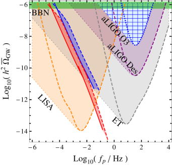
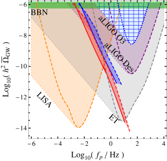
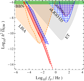
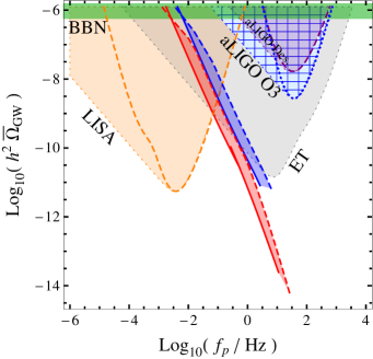
Figure 7: Experimental parameter reach in the $\{h^{2}\overline{\Omega}_{\textrm{\tiny GW}},f_{p}\}$ plane for SGWBs in the regimes $\Omega_{\textrm{\tiny GW}}^{\rm env}$ (regions inside dotted borders) and $\Omega_{\textrm{\tiny GW}}^{\rm sw}$ (regions inside dashed borders). Diagonal strips are for $N=10$ (red), $25$ (blue) for $\rho=1$ TeV (left panels), $\rho=100$ TeV (right panels), SNR $\geq 2$ (upper panels) and SNR $\geq 1000$ (lower panels). Solid and dashed lines on the edge of the strips correspond to the regime $\overline{\Omega}_{\textrm{\tiny GW}}\simeq\overline{\Omega}_{\textrm{\tiny GW}}^{\rm env}$ and $\overline{\Omega}_{\textrm{\tiny GW}}^{\rm sw}$, respectively. Shadowed (green) regions in both panels are excluded by BBN. We have considered for the wall velocity $v_{\omega}\simeq 0.99$.

We also analyze values of $\rho>100$ TeV which do not appear in Fig. 7. Taking into account that $m_{\textrm{\tiny KK}}/\rho\simeq 3.88$ as discussed in Sec. 3.3, we find that values of $m_{\textrm{\tiny KK}}\sim\mathcal{O}(10^{4})\,$ – $\mathcal{O}(10^{7})\,$TeV are being already cornered by current aLIGO O3 data. The forecast shows that by the early 2040s the ground-based and space-based interferometer network will be sensitive to a huge parameter region, reaching the following KK scales: $m_{\textrm{\tiny KK}}\lesssim 10^{5}$ TeV in LISA, $10^{2}~{}\textrm{TeV}\lesssim m_{\textrm{\tiny KK}}\lesssim 10^{8}$ TeV in LIGO-like detectors, and $m_{\textrm{\tiny KK}}\lesssim 10^{9}$ TeV in ET. Most of the SGWB signals are so inside the sensitivity curves that they are expected to be reconstructed with a very high accuracy, shedding light on the scale of new physics [30, 31, 32].

6 Conclusions

We have studied warped models with a radion stabilized with a polynomial bulk potential, and addressed the computation of the radion effective potential at zero and finite temperature. The zero temperature computation has been carried out by adopting a recent technique that allows for a sizable backreaction on the gravitational metric. In the limit of small backreaction, our findings are in good agreement with previous results in the literature, as for instance the original Goldberger-Wise potential [14]. At finite temperature, the radion undergoes a first order phase transition which, in the four-dimensional language, can be seen as a confinement/deconfinement phase transition. We have found that the radion phase transition potentially generates a SGWB signal which covers several gravitational wave frequency bands. In particular, it can be often detected at both ground-based and space-based gravitational wave interferometers with a high signal-to-noise ratio, enabling an accurate signal reconstruction at completely different frequency ranges. In view of the correct LHC constraints, we have considered the possibility of Kaluza-Klein resonance masses much heavier than the TeV scale, thus leaving open the door for a little hierarchy problem and the corresponding level of fine-tuning. By recasting the sensitivity region of the gravitational wave detector network, we have found that in the next two decades the gravitational wave detectors will broadly probe warped models with resonances up to $m_{\textrm{\tiny KK}}\lesssim 10^{9}\,\textrm{TeV}$. However, the most interesting detection prospects seem to be those for the region $1\,\textrm{TeV}\ll m_{\textrm{\tiny KK}}\lesssim 100\,\textrm{TeV}$, which deserves a future, dedicated study. In fact, for this region, the synergy between gravitational wave and collider experiments is exciting.

References

References

- [1] L. Randall, R. Sundrum, A Large mass hierarchy from a small extra dimension, Phys. Rev. Lett. 83 (1999) 3370–3373.
- [2] A. M. Sirunyan, et al., Search for resonant production in proton-proton collisions at TeV, JHEP 04 (2019) 031.
- [3] M. Aaboud, et al., Search for heavy particles decaying into a top-quark pair in the fully hadronic final state in collisions at 13 TeV with the ATLAS detector, Phys. Rev. D99 (9) (2019) 092004.
- [4] P. Creminelli, A. Nicolis, R. Rattazzi, Holography and the electroweak phase transition, JHEP 03 (2002) 051.
- [5] L. Randall, G. Servant, Gravitational waves from warped spacetime, JHEP 05 (2007) 054.
- [6] G. Nardini, M. Quiros, A. Wulzer, A Confining Strong First-Order Electroweak Phase Transition, JHEP 09 (2007) 077.
- [7] C. Caprini, et al., Science with the space-based interferometer eLISA. II: Gravitational waves from cosmological phase transitions, JCAP 1604 (04) (2016) 001.
- [8] W. D. Goldberger, M. B. Wise, Bulk fields in the Randall-Sundrum compactification scenario, Phys. Rev. D60 (1999) 107505.
- [9] C. Csaki, M. L. Graesser, G. D. Kribs, Radion dynamics and electroweak physics, Phys. Rev. D63 (2001) 065002.
- [10] J. A. Cabrer, G. von Gersdorff, M. Quiros, Suppressing Electroweak Precision Observables in 5D Warped Models, JHEP 05 (2011) 083.
- [11] E. Megias, G. Nardini, M. Quiros, Cosmological Phase Transitions in Warped Space: Gravitational Waves and Collider Signatures, JHEP 09 (2018) 095.
- [12] M. Carena, E. Megias, M. Quiros, C. Wagner, in custodial warped space, JHEP 12 (2018) 043.
- [13] E. Megias, G. Nardini, M. Quiros, Gravitational Imprints from Heavy Kaluza-Klein Resonances, Phys. Rev. D102 (5) (2020) 055004.
- [14] W. D. Goldberger, M. B. Wise, Modulus stabilization with bulk fields, Phys. Rev. Lett. 83 (1999) 4922–4925.
- [15] I. Papadimitriou, Multi-Trace Deformations in AdS/CFT: Exploring the Vacuum Structure of the Deformed CFT, JHEP 05 (2007) 075.
- [16] E. Megias, O. Pujolas, Naturally light dilatons from nearly marginal deformations, JHEP 08 (2014) 081.
- [17] J. M. Lizana, M. Olechowski, S. Pokorski, A new way of calculating the effective potential for a light radion, JHEP 09 (2020) 092.
- [18] E. Megias, O. Pujolas, M. Quiros, On dilatons and the LHC diphoton excess, JHEP 05 (2016) 137.
- [19] S. R. Coleman, The Fate of the False Vacuum. 1. Semiclassical Theory, Phys. Rev. D15 (1977) 2929–2936, [erratum: Phys. Rev. D16, 1248(1977)].
- [20] A. D. Linde, Fate of the False Vacuum at Finite Temperature: Theory and Applications, Phys. Lett. 100B (1981) 37–40.
- [21] T. Konstandin, G. Nardini, M. Quiros, Gravitational Backreaction Effects on the Holographic Phase Transition, Phys. Rev. D82 (2010) 083513.
- [22] D. Bunk, J. Hubisz, B. Jain, A Perturbative RS I Cosmological Phase Transition, Eur. Phys. J. C78 (1) (2018) 78.
- [23] S. J. Huber, T. Konstandin, Gravitational Wave Production by Collisions: More Bubbles, JCAP 0809 (2008) 022.
- [24] M. Hindmarsh, S. J. Huber, K. Rummukainen, D. J. Weir, Shape of the acoustic gravitational wave power spectrum from a first order phase transition, Phys. Rev. D96 (10) (2017) 103520, [erratum: Phys. Rev. D101, no.8, 089902(2020)].
- [25] C. Caprini, et al., Detecting gravitational waves from cosmological phase transitions with LISA: an update, JCAP 03 (2020) 024.
- [26] H.-K. Guo, K. Sinha, D. Vagie, G. White, Phase Transitions in an Expanding Universe: Stochastic Gravitational Waves in Standard and Non-Standard Histories, JCAP 2101 (2021) 001.
- [27] M. B. Hindmarsh, M. Lüben, J. Lumma, M. Pauly, Phase transitions in the early universe, SciPost Phys. Lect. Notes 24 (2021) 1.
- [28] F. R. Ares, M. Hindmarsh, C. Hoyos, N. Jokela, Gravitational waves from a holographic phase transition, arXiv:2011.12878.
- [29] R. Abbott, et al., Upper Limits on the Isotropic Gravitational-Wave Background from Advanced LIGO’s and Advanced Virgo’s Third Observing Run, arXiv:2101.12130.
- [30] D. G. Figueroa, E. Megias, G. Nardini, M. Pieroni, M. Quiros, A. Ricciardone, G. Tasinato, LISA as a probe for particle physics: electroweak scale tests in synergy with ground-based experiments, PoS GRASS2018 (2018) 036.
- [31] C. Caprini, D. G. Figueroa, R. Flauger, G. Nardini, M. Peloso, M. Pieroni, A. Ricciardone, G. Tasinato, Reconstructing the spectral shape of a stochastic gravitational wave background with LISA, JCAP 11 (2019) 017.
- [32] R. Flauger, N. Karnesis, G. Nardini, M. Pieroni, A. Ricciardone, J. Torrado, Improved reconstruction of a stochastic gravitational wave background with LISA, JCAP 01 (2021) 059.