A transiting warm giant planet around the young active star TOI-201

Abstract

We present the confirmation of the eccentric warm giant planet TOI-201 b, first identified as a candidate in TESS photometry (Sectors 1-8, 10-13, and 27-28) and confirmed using ground-based photometry from NGTS and radial velocities from FEROS, HARPS, CORALIE, and Minerva-Australis. TOI-201 b orbits a young ($\mathrm{0.87^{+0.46}_{-0.49}\,Gyr}$) and bright(V=9.07 mag) F-type star with a $\mathrm{52.9781\,d}$ period. The planet has a mass of $\mathrm{0.42^{+0.05}_{-0.03}\,M_{J}}$, a radius of $\mathrm{1.008^{+0.012}_{-0.015}\,R_{J}}$, and an orbital eccentricity of $0.28^{+0.06}_{-0.09}$; it appears to still be undergoing fairly rapid cooling, as expected given the youth of the host star. The star also shows long-term variability in both the radial velocities and several activity indicators, which we attribute to stellar activity. The discovery and characterization of warm giant planets such as TOI-201 b is important for constraining formation and evolution theories for giant planets.

1 Introduction

Transiting warm giants - that is, planets with $\mathrm{R_{P}\gtrsim 0.8\,R_{J}}$ and $\mathrm{10\,d\lesssim P\lesssim 100\,d}$ - are particularly important for understanding the formation and evolution of giant planets. Unlike hot Jupiters - i.e., planets with $\mathrm{R_{P}\gtrsim 0.8\,R_{J}}$ and $\mathrm{P\lesssim 10\,d}$ - which are inflated by mechanisms that are still unclear but likely connected to irradiation (e.g. Sarkis et al., 2020) these more distant planets are less strongly irradiated by their host star, meaning their size and mass can be effectively modelled by their metallicity (e.g. Thorngren & Fortney, 2019). Both hot and warm Jupiters are unlikely to form in situ, but rather are expected to have formed in the outer regions of the disk and migrated to their current locations; the main mechanisms proposed are gas disk migration and high eccentricity migration (see Dawson & Johnson 2018 for a comprehensive review). However, hot Jupiters’ orbital histories are affected by tidal evolution, which can erase traces of past interactions between planets; this is not the case for warm Jupiters. Therefore, this population of planets preserves valuable information for the study of giant planet formation in their physical and orbital parameters. These parameters can be characterized through the combination of photometry and radial velocities.

While the current sample of warm giants is still small, the Transiting Exoplanet Survey Satellite (TESS, Ricker et al., 2015) is expected to detect hundreds of such planets (Sullivan et al., 2015; Barclay et al., 2018). The Warm gIaNts with tEss collaboration (WINE, e.g. Brahm et al., 2019; Jordán et al., 2020a) is using a network of photometric and spectroscopic facilities to follow up, confirm, and characterize warm giant candidates from TESS. One such candidate is TOI-201.01.

In this paper, we present the confirmation and characterization of the warm giant TOI-201 b, orbiting the young F-type star TOI-201. The paper is organized as follows. We present the observational data in Section 2. In Section 3 we analyse the data, and characterize the star and planet. Finally, our results are discussed in Section 4.

2 Observations

2.1 Photometric data

2.1.1 TESS

TOI-201 was observed by the TESS mission between 25 July 2018 and 17 July 2019, in Sectors 1, 2, 3, 4, 5, 6, 7, 8, 10, 11, 12, and 13, using camera 4. CCD 1 was used for Sectors 3, 4, and 5; CCD 2 for Sectors 6, 7, and 8; CCD 3 for Sectors 10, 11, and 12; and CCD 4 for Sectors 1, 2, and 13. Currently, it is also being observed as part of the extended mission; the light curves from Sectors 27 and 28, which were observed between 5 July and 25 August 2020, were also incorporated into the analysis. Camera 4 in CCD 4 was used for both these Sectors.

The 2-minute cadence data for TOI-201 were processed in the TESS Science Processing Operation Center (SPOC, Jenkins et al., 2016) pipeline. Two potential transit signals were identified in the SPOC transit search (Jenkins, 2002; Jenkins et al., 2010, 2020) of the TOI-201 light curve. These were designated as TESS Objects of Interest (TOIs) by the TESS Science Office based on SPOC data validation results (Twicken et al., 2018; Li et al., 2019) indicating that both signals were consistent with transiting planets. The planetary candidates are listed in the ExoFOP-TESS archive: TOI-201.01, with a period of $\mathrm{P_{01}=52.978306\,d}$, and TOI-201.02, with a period of $\mathrm{P_{02}=5.849173\,d}$. The full PDCSAP light curve (Stumpe et al., 2012, 2014; Smith et al., 2012), obtained from the MAST archive, is shown in Fig. 1 (top panel). Any points that were flagged as being of low quality have been removed. Six full transits of TOI-201.01 are clearly visible, in Sectors 2, 4, 6, 10, 12, and 28. A partial transit is also visible in Sector 8, at the edge of a five day gap in the light curve (Fig. 1, bottom panel). This gap is due to an instrument turn-off between TJD 1531.74 and TJD 1535.00, caused by an interruption in communications between the instrument and spacecraft. The flux is clearly overestimated for the first $\mathrm{\sim 0.5\,d}$ after the gap. This artifact appears to have been introduced in the SPOC PDC processing, as the SAP light curve shows a low flux level for this period, which is likely due to the camera temperature change of $\mathrm{\sim 20^{\circ}}$ during the instrument turn-off, as detailed in the TESS Data Release Notes for Sector 8, DR10. The transits of TOI-201.02 have a much shallower depth (only $\mathrm{0.128\pm 0.013\,mmag}$, compared to $\mathrm{6.843\pm 0.058\,mmag}$ for TOI-201.01), and are hence not visually obvious in the light curve.

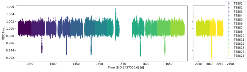
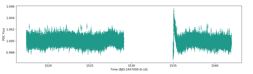
Figure 1: Top: TESS light curve for TOI-201, for all Sectors. The data are colour-coded by Sectors, and flagged points have been removed. The left subplot shows the twelve Sectors from the prime mission, and the right subplot the two Sectors from the extended mission. Bottom: Zoom to Sector 8, showing the 5-day gap in the light curve, and the partial transit of TOI-201.01 at the edge of the gap.

2.1.2 NGTS

Due to the relatively large $21\arcsec$ pixel size of TESS, nearby companions can contaminate its photometry. It is therefore necessary to identify possible contaminating sources, which can create false positives or dilute the transits. Ground-based photometry plays an important role in disentangling these false positives. In this context, The Next Generation Transit Survey (NGTS, Wheatley et al., 2018) observed TOI-201 on 19th September 2019, obtaining a clear ingress signal (Fig. 2). Two telescopes were used, with the custom NGTS filter (520-890 nm). A total of 2484 images were obtained with an exposure time of 10 seconds, for an overall cadence (exposure, read out, etc.) of 13 seconds. The images were reduced with a custom aperture photometry pipeline (Bryant et al., 2020), using an aperture with a radius of 7 pixels ($35\arcsec$).

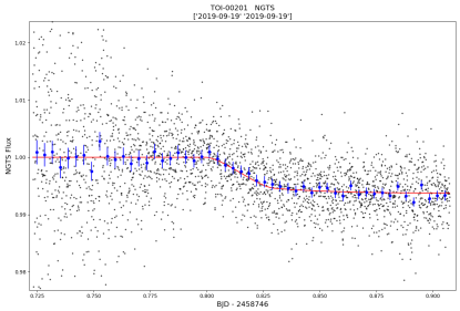
Figure 2: NGTS light curve for TOI-201, observed on 19th September 2019. The blue points show the data binned to 5 minutes. The red line indicates the predicted model from the TESS data, using ephemeris of $\mathrm{T_{0}=1376.052045}$, $\mathrm{P=52.978306\,d}$.

2.2 High-resolution imaging

High-resolution imaging is a valuable tool for rejecting false positive scenarios for TESS candidates. In this context, the SOAR TESS survey (Ziegler et al., 2020) has observed TESS planet candidate hosts with speckle imaging using the high-resolution camera (HRCam) imager on the 4.1-m Southern Astrophysical Research (SOAR) telescope at Cerro Pachón, Chile (Tokovinin, 2018). TOI-201 was observed on the night of 18 February 2019, with no nearby sources detected within $3\arcsec$. The contrast curve and auto-correlation function are shown in Fig. 3.

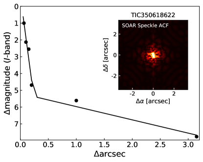
Figure 3: Contrast curve and speckle auto-correlation function from the HRCam at SOAR for TOI-201. The black points and solid line indicate the $5\sigma$ contrast curve; the inset shows the speckle auto-correlation function.

2.3 Spectroscopic data

The WINE consortium carried out spectroscopic follow-up of TOI-201 with the FEROS and HARPS spectrographs. In addition to these, we also obtained data from the CORALIE and Minerva-Australis teams. Finally, TOI-201 was observed once with NRES, for the purpose of stellar parameter determination.

2.3.1 FEROS

We obtained 52 spectra with the FEROS spectrograph (Kaufer et al., 1999), which is mounted on the MPG 2.2m telescope at La Silla Observatory and has a resolving power of $\mathrm{R=50\,000}$, between 26 November 2018 and 8 March 2020. The observations were performed in the Object-Calibration mode, with an exposure time of 5 minutes. The spectra, which have a median signal to noise ratio (SNR) of 165, were processed with the CERES pipeline (Brahm et al., 2017a). From this pipeline, we obtain both radial velocities (RV) and activity indicators. Specifically, we compute the bisector of the CCF (BIS), which traces photospheric activity (e.g. Queloz et al., 2001a), and the H_α, log($R^{\prime}_{HK}$), Na II, and He I activity indices, which trace chromospheric activity. For H_α, we used the definition of Boisse et al. (2009). As TOI-201 is an F-type star, we used the regions defined by Duncan et al. (1991) and the calibrations of Noyes et al. (1984) for log($R^{\prime}_{HK}$). For Na II and He I we followed Gomes da Silva et al. (2011). The radial velocities and activity indices computed from the FEROS data are listed in table 6; the RVs have a median error of $\mathrm{\sigma_{RV}\approx 9.1\,m/s}$.

2.3.2 HARPS

We obtained 39 spectra with the HARPS spectrograph (Mayor et al., 2003), which is mounted on the 3.6m telescope at La Silla Observatory, and has a resolving power of $\mathrm{R=120\,000}$. The spectra were obtained between 11 December 2018 and 21 February 2020, under Program IDs 0101.C-0510(D), 0102.C-0451(B), 0103.C-0442(A), and 0104.C-0413(A). The exposures were taken in simultaneous sky mode, with a 10 minute duration. One observation, obtained on 17 January 2020, has an extremely low SNR of 17 and was therefore removed from the analysis. The remaining 38 spectra have a median SNR of 109. As with the FEROS spectra, we processed the HARPS spectra using the CERES pipeline, obtaining the radial velocities and the same set of activity indicators. The radial velocities and activity indices computed from the HARPS data are listed in table 7; the RVs have a median error of $\mathrm{\sigma_{RV}\approx 2.0\,m/s}$.

2.3.3 CORALIE

A total of 10 spectra of TOI-201 were obtained with the CORALIE high resolution spectrograph on the Swiss 1.2 m Euler telescope at La Silla Observatories, Chile (Queloz et al., 2001b), between 12 November 2018 and 27 March 2019. Each exposure had a duration of 20 minutes yielding a SNR of $\sim 45$. CORALIE is a fibre-fed echelle spectrograph with a $2\arcsec$ science fibre and a secondary fibre with a Fabry-Perot for simultaneous wavelength calibration. We extract radial velocity measurements by cross-correlation of the spectra with a binary G2V template (Baranne et al., 1996; Pepe et al., 2002). We obtain final RV uncertainties for the CORALIE epochs of $\mathrm{\sigma_{RV}\approx 10-15\,m/s}$. BIS, FWHM and other line-profile diagnostics were computed as well using the standard CORALIE DRS. We also compute the $\mathrm{H_{\alpha}}$ index for each spectrum to check for possible variation in stellar activity. We investigate various scenarios where a blended eclipsing stellar binary can mimic a transiting planet using the line profile diagnostics and find no evidence of such.

2.3.4 Minerva-Australis

Minerva-Australis is an array of four PlaneWave CDK700 telescopes located in Queensland, Australia, fully dedicated to the precise radial-velocity follow-up of TESS candidates (e.g. Addison et al., 2020a, b; Jordán et al., 2020b). The four telescopes can be simultaneously fiber-fed to a single KiwiSpec R4-100 high-resolution ($\mathrm{R=80\,000}$) spectrograph (Barnes et al., 2012; Addison et al., 2019). We obtained 62 spectra of TOI-201 in the early days of Minerva-Australis, with a single telescope, between 2 January 2019 and 15 April 2019. Exposure times were 30 minutes, and on some nights, two consecutive exposures were obtained. The resulting radial velocities are given in Table  9. Radial velocities for the observations are derived for each telescope by cross-correlation, where the template being matched is the mean spectrum of each telescope. The instrumental variations are corrected by using simultaneous Thorium-Argon arc lamp observations.

2.3.5 NRES

The Network of Robotic Echelle Spectrographs (NRES, Siverd et al., 2018) of the Las Cumbres Observatory (LCOGT, Brown et al., 2013) consists of four identical fibre-fed optical echelle spectrographs, with a resolving power of $\mathrm{R\approx 53\,000}$, mounted on globally distributed 1 m telescopes. TOI-201 was observed by NRES at CTIO on 8 December 2018. A SpecMatch analysis (Yee et al., 2017) was performed on the spectrum, yielding the following stellar parameters: $\mathrm{T_{eff}=6280\pm 100\,K}$, $\mathrm{\log{g}=4.3\pm 0.1}$, $\mathrm{Fe/H=0.21\pm 0.06}$, $\mathrm{v\sin{i}=8.4\pm 2.1\,kms^{-1}}$, $\mathrm{M_{\star}=1.285\pm 0.064\,M_{\odot}}$, and $\mathrm{R_{\star}=1.35\pm 0.17\,R_{\odot}}$.

3 Analysis

3.1 Stellar parameters

In order to characterise the host star, we first used the co-added HARPS spectra to determine the atmospheric parameters. We employed the ZASPE code (Brahm et al., 2017b), which compares the observed spectrum to a grid of synthetic models generated from the ATLAS9 model atmospheres (Castelli & Kurucz, 2003) in order to determine the effective temperature $\mathrm{T_{eff}}$, surface gravity $\mathrm{\log{g}}$, metallicity [Fe/H], and projected rotational velocity $\mathrm{v\sin{i}}$.

Next, we followed the second procedure described in Brahm et al. (2019) to determine the physical parameters. To summarize, we compare the broadband photometric measurements, converted to absolute magnitudes using the Gaia DR2 (Gaia Collaboration et al., 2016, 2018) parallax, with the stellar evolutionary models of Bressan et al. (2012). We use the emcee package (Foreman-Mackey et al., 2013) to sample the posterior distributions. Through this procedure, we determine the age, mass, radius, luminosity, density, and extinction. We also obtain new values for $\mathrm{T_{eff}}$ and $\mathrm{\log{g}}$, the latter of which is more precise than the one previously determined through ZASPE. Therefore, we iterate the entire procedure, using the new $\mathrm{\log{g}}$ as an additional input parameter for ZASPE. One iteration was sufficient for the $\mathrm{\log{g}}$ value to converge. The stellar parameters and observational properties of TOI-201 are presented in Table 1. The quoted error bars for the stellar parameters are internal errors, computed as the $\pm 1\sigma$ interval around the median of the posterior for each parameter; they do not take into account any systematic errors on the stellar models. The parameters we derive are consistent at one sigma with those obtained from the NRES spectrum (Section 2.3.5). We find that TOI-201 is a young, F-type star.

Table 1: Stellar parameters of TOI-201.

Parameter	Value	Reference
Names	HD 39474
	TIC 350618622, TOI-201	TESS
	J05493641-5454386	2MASS
	4767547667180525696	Gaia DR2
RA (J2000)	$05^{h}49^{m}36.4138946584^{s}$	Gaia DR2
DEC (J2000)	$-54^{h}54^{m}38.552783926^{s}$	Gaia DR2
pmRA [mas yr-1]	7.731 $\pm$ 0.052	Gaia DR2
pmDEC [mas yr-1]	66.448 $\pm$ 0.058	Gaia DR2
$\pi$ [mas]	8.7566 $\pm$ 0.0265	Gaia DR2
T [mag]	8.5822$\pm$ 0.006	TESS
B [mag]	10.104 $\pm$ 0.055	APASS
V [mag]	9.715 $\pm$ 0.079	APASS
J [mag]	8.103 $\pm$ 0.029	2MASS
H [mag]	7.923 $\pm$ 0.036	2MASS
Ks [mag]	7.846 $\pm$ 0.024	2MASS
$T_{\rm eff}$ [K]	6394 $\pm$ 75	this work
Spectral type	F6V	PM13
Fe/H [dex]	0.240 $\pm$ 0.036	this work
$\log{g}$ [dex]	4.318 $\pm$ 0.014	this work
$v\sin{i}$ [$\mathrm{kms^{-1}}$]	9.52 $\pm$ 0.278	this work
R⋆ [R⊙]	1.317 $\pm$ 0.011	this work
M⋆ [M⊙]	1.316 $\pm$ 0.027	this work
L⋆ [L⊙]	2.6 $\pm$ 0.1	this work
$\rho_{\star}$ [g cm-3]	0.81 $\pm$ 0.03	this work
Age [Gyr]	$0.87^{+0.46}_{-0.49}$	this work
AV [mag]	0.11 $\pm$ 0.05	this work
$\log R^{\prime}_{\rm hk}$	-4.76 $\pm$ 0.04	this work

TESS: TESS Input Catalog (Stassun, 2019); 2MASS: Two-micron All Sky Survey (Skrutskie et al., 2006); Gaia DR2: Gaia Data Release 2 (Gaia Collaboration et al., 2016, 2018); APASS: AAVSO Photometric All-Sky Survey (Munari et al., 2014); PM13: using the tables of Pecaut & Mamajek (2013).

3.2 Radial velocity analysis

In this section, we present the analysis of the FEROS and HARPS spectra, all of which were processed using the CERES pipeline. For homogeneity, we do not include the CORALIE and Minerva-Australis data in this section, as they were processed using the respective instrument pipelines. Additionally, the FEROS and HARPS data have longer temporal baselines, covering both the 2018-2019 and 2019-2020 observing seasons, whereas CORALIE and Minerva-Australis only observed TOI-201 during the 2018-2019 season.

The GLS periodograms of the joint FEROS and HARPS RV and activity indices time series are presented in Figure 4. The $\mathrm{52.9\,d}$ period of the planetary candidate TOI-201.01 is highlighted. There is a clear, highly significant peak close to this period in the RV periodogram, as well as several significant long-period peaks. We do not find significant peaks close to $\mathrm{\sim 53\,d}$ for any of the activity indices, indicating that the signal in the RVs is likely to be planetary in nature. On the other hand, there are several short- and long-term signatures in the activity indices. There is no clear rotation period in the light curve according to Canto Martins et al. (2020), but given the radius and $v\sin{i}$ reported in Table 1, we may expect a period of $\mathrm{\sim 7\,d}$ (assuming no misalignment); there is a peak at $\mathrm{\sim 8\,d}$ in the RVs, and hints of peaks at the same period in the log($R^{\prime}_{HK}$) Na II and He I periodograms. There are also long-period peaks at $\mathrm{\sim 300\,d}$ in both the H_α and log($R^{\prime}_{HK}$) periodograms, similar to the one seen in the RVs. Additionally, there are peaks at $\mathrm{\sim 40\,d}$ in the Na II and He I periodograms, with no obvious correspondence in the RVs.

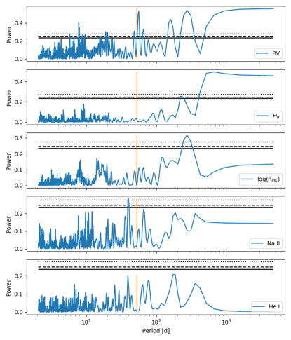
Figure 4: GLS Periodograms of the joint FEROS-HARPS time series for (top to bottom) radial velocities, H_α, log($R^{\prime}_{HK}$), Na II, and He I. The solid, dashed, and dotted horizontal black lines indicate the 1%, 0.5% and 0.01% FAP levels respectively. The vertical orange line indicates the period of the planetary candidate TOI-201.01.

Correlations between the bisector spans and the radial velocities can also indicate a stellar origin for radial velocity variations (e.g. Queloz et al., 2001a). The radial velocity measurements are plotted against the bisector spans in Figure 5 for both FEROS and HARPS data. Spearman correlation tests indicate no significant correlation between the bisector spans and the radial velocities, nor between the bisector spans and the orbital phases of TOI-201.01, for either data-set: For FEROS, we find a Spearman correlation coefficient $r_{s}=-0.31$ with $p\mathrm{\textnormal{-}value}=0.03$ between the RVs and bisector spans, and $r_{s}=-0.02$ with $p\mathrm{\textnormal{-}value}=0.09$ between the orbital phases and bisector spans; for HARPS, we find $r_{s}=0.15$ with $p\mathrm{\textnormal{-}value}=0.38$ between the RVs and bisector spans, and $r_{s}=-0.13$ with $p\mathrm{\textnormal{-}value}=0.44$ between the orbital phases and bisector spans.

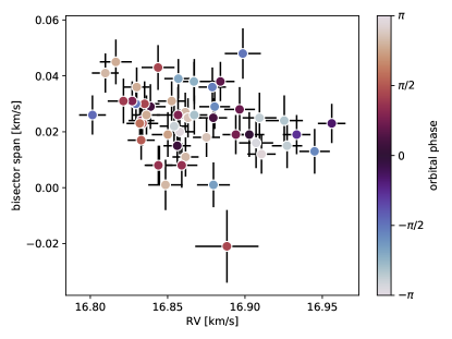
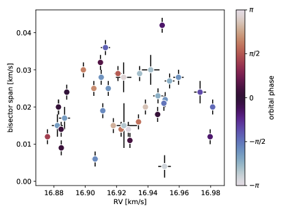
Figure 5: Bisector span as a function of radial velocity, for FEROS (top) and HARPS (bottom) data. The points are colour-coded by orbital phase. No correlations are apparent.

In order to further verify that the $\mathrm{\sim 53\,d}$ signal is planetary in nature, we also computed the Phase Distance Correlation (PDC) periodogram (Zucker, 2018) for the FEROS data. We find a stronger signal at the $\mathrm{53\,d}$ period in the PDC periodogram than in a comparison GLS periodogram, as expected for eccentric orbits, as shown in Fig. 6. We also ran the recent PDC extension, the USuRPER (Binnenfeld et al., 2020), which is designed to account for fluctuations in the entire spectral shape. A prominent peak is visible in the USuRPER low frequency region (Fig. 6). This result strengthens the finding that those signals are caused by some sort of periodic variations in the spectral feature shape. Both the PDC and USuRPER periodograms are implemented in the SPARTA code library (Shahaf et al., 2020).

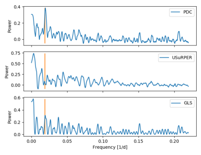
Figure 6: PDC (top), USuRPER (middle), and, for comparison, GLS (bottom) periodograms of the joint FEROS-HARPS RV time series. The vertical orange line indicates the period of the planetary candidate TOI-201.01. The peak at the planetary period is enhanced in the PDC periodogram compared to the GLS periodogram, and suppressed in the USuRPER periodogram which shows a peak in low frequencies.

We use the juliet python package (Espinoza et al., 2019) to model the joint FEROS and HARPS radial velocities. This tool allows us to jointly fit photometric data (using the batman package, Kreidberg 2015) and radial velocities (using the radvel package, Fulton et al. 2018), and also to incorporate Gaussian Processes (via the celerite package, Foreman-Mackey et al. 2017). The parameter space is explored through nested sampling, using the MultiNest algorithm (Feroz et al., 2009) in its python implementation, PyMultiNest (Buchner et al., 2014), or the dynesty package (Speagle, 2020).

We tested six models for the radial velocities: A flat model with no Keplerian components; a single circular planet; a single eccentric planet; two eccentric planets; a single eccentric planet plus a quadratic trend to model long-term effects; and a single eccentric planet plus a Gaussian process (GP) to account for stellar activity. The full priors for each model are listed in Table 2, and the posteriors in Table 3. For all Keplerian components, we used the periods $\mathrm{P_{01},\,P_{02}}$ and epochs $\mathrm{T0_{01},\,T0_{02}}$ listed in ExoFOP-TESS for candidates TOI-201.01 and TOI-201.02 respectively as initial constraints. For eccentric models, we use the ($\mathrm{e\sin{\omega},\,e\cos{\omega}}$) parametrization.

1. no planet: this model assumes that all the RV variations are due solely to jitter. The only free parameters are the systemic radial velocities and jitters for the two instruments. This model effectively provides us with a baseline log-evidence $\ln(Z)=32.9\pm 0.2$.

2. one-planet, circular: in this model, we add a Keplerian with Gaussian priors for the period and T0 centred on those provided by the light curve, and an eccentricity fixed to zero. We find a surprisingly low log-evidence of $\ln(Z)=1.16\pm 0.02$. As can be seen in Table 3, the instrumental jitter values are very similar to those of the flat model, suggesting that the RV variations may be absorbed by this jitter.

3. one-planet, eccentric: in this model, we allow for free eccentricity and $\omega$ for the Keplerian. We find a much higher log-evidence of $\ln(Z)=126.7\pm 0.1$.

4. two planets, eccentric: In addition to the Keplerian with priors centred on the parameters of TOI-201.01, we include a second Keplerian (also with free eccentricity and $\omega$) to represent TOI-201.02. We find a decreased log-evidence with respect to model 3 of $\ln(Z)=25.96\pm 0.01$, and the eccentricity for the 53 d Keplerian is increased.

5. one-planet, eccentric, plus quadratic trend: in this model, we test the inclusion of a quadratic trend to model long-term effects. The intercept parameter is fixed to zero, as otherwise it becomes degenerate with the instrumental offsets. We find a log-evidence of $\ln(Z)=173.60\pm 0.01$.

6. one-planet, eccentric, plus GP: in this model, we incorporate a Gaussian process, to account for stellar activity. We use an (approximate) Matern kernel, as implemented in celerite. We find a log-evidence of $\ln(Z)=185.71\pm 0.02$.

The model with a single eccentric Keplerian and a Gaussian process is clearly favoured, with a $\Delta\ln Z_{\ref*{mod:rv-1ple-gp},\ref*{mod:rv-1ple}}\approx 59$ compared to the model with only a single eccentric planet, and better accounts for other trends in the data, with $\Delta\ln Z_{\ref*{mod:rv-1ple-gp},\ref*{mod:rv-1ple-qu}}\approx 12$ compared to the model with a single eccentric planet and a quadratic trend. Likewise, the difference to the flat model is of $\Delta\ln Z_{\ref*{mod:rv-1ple-gp},\ref*{mod:rv-no-planet}}\approx 153$. This allows us to confirm the candidate planet TOI-201.01, referred to as TOI-201 b hereafter. The full model and components, and the FEROS and HARPS RVs, are shown in Fig. 7.

Table 2: Prior parameter distributions for the RV analysis. $\mathcal{U}(a,b)$ indicates a uniform distribution between $a$ and $b$; $\mathcal{N}(a,b)$ a normal distribution with mean $a$ and standard deviation $b$; $\mathcal{J}(a,b)$ a Jeffreys or log-uniform distribution between $a$ and $b$.

Parameter	Distribution	Models
$\mu_{\mathrm{{HARPS}}}$ [km/s]	$\mathcal{U}(-30,30)$	1, 2, 3, 4, 5, 6
$\mu_{\mathrm{{FEROS}}}$ [km/s]	$\mathcal{U}(-30,30)$	1, 2, 3, 4, 5, 6
$\sigma_{\mathrm{{HARPS}}}$ [km/s]	$\mathcal{J}(0.001,100)$	1, 2, 3, 4, 5, 6
$\sigma_{\mathrm{{FEROS}}}$ [km/s]	$\mathcal{J}(0.001,100)$	1, 2, 3, 4, 5, 6
P01 [d]	$\mathcal{N}(52.978306,0.1)$	2, 3, 4, 5, 6
T001 [d]	$\mathcal{N}(2458376.052124,0.1)$	2, 3, 4, 5, 6
K01 [km/s]	$\mathcal{U}(0,1)$	2, 3, 4, 5, 6
$e\sin{\omega}_{\mathrm{01}}$	$\mathcal{U}(-1,1)$	3, 4, 5, 6
$e\cos{\omega}_{\mathrm{01}}$	$\mathcal{U}(-1,1)$	3, 4, 5, 6
P02 [d]	$\mathcal{N}(5.849173,0.1)$	4
T002 [d]	$\mathcal{N}(2458327.244194,0.1)$	4
K02 [km/s]	$\mathcal{U}(0,1)$	4
$e\sin{\omega}_{\mathrm{02}}$	$\mathcal{U}(-1,1)$	4
$e\cos{\omega}_{\mathrm{02}}$	$\mathcal{U}(-1,1)$	4
$rv_{slope}$ [(km/s)/d]	$\mathcal{U}(-100,100)$	5
$rv_{quad}$ [(km/s)/d2]	$\mathcal{U}(-100,100)$	5
$\sigma_{\mathrm{{GP}}}$	$\mathcal{J}(0.01,100)$	6
$\rho_{\mathrm{{GP}}}$	$\mathcal{J}(0.01,100)$	6

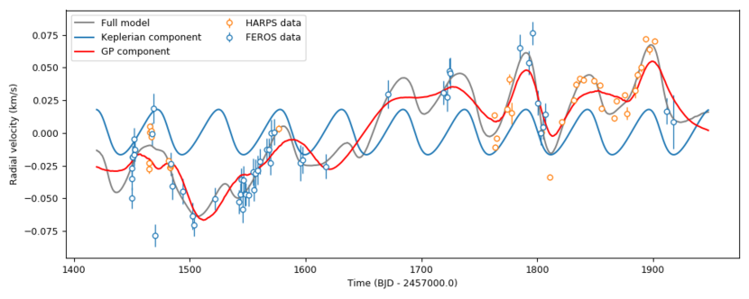
Figure 7: RV data for FEROS and HARPS, full fitted model, and Keplerian and GP model components, for the favoured model of one eccentric planet plus a Gaussian process.

Table 3: RV analysis for the different models tested. Top: posterior parameter distributions. Bottom: log-evidence and difference to the baseline no-planet model. Model 6 is the final adopted model.

Parameter	Flat model (1)	1 planet circ. (2)	1 planet ecc. (3)	2 planet ecc. (4)	1 planet + quad (5)	1 planet + GP (6)
$\mu_{\mathrm{{HARPS}}}$ [km/s]	$16.999^{+0.009}_{-0.038}$	$16.92^{+0.01}_{-0.01}$	$16.92^{+0.01}_{-0.01}$	$17.04^{+0.04}_{-0.05}$	$16.884^{+0.003}_{-0.004}$	$16.91^{+0.05}_{-0.06}$
$\mu_{\mathrm{{FEROS}}}$ [km/s]	$16.983^{+0.010}_{-0.002}$	$16.834^{+0.004}_{-0.003}$	$16.875^{+0.005}_{-0.006}$	$16.89^{+0.01}_{-0.01}$	$16.855^{+0.003}_{-0.004}$	$16.88^{+0.05}_{-0.06}$
$\sigma_{\mathrm{{HARPS}}}$ [km/s]	$0.148^{+0.007}_{-0.009}$	$0.157^{+0.003}_{-0.003}$	$0.068^{+0.012}_{-0.008}$	$0.40^{+0.05}_{-0.04}$	$0.011^{+0.002}_{-0.001}$	$0.012^{0.001}_{0.001}$
$\sigma_{\mathrm{{FEROS}}}$ [km/s]	$0.189^{+0.013}_{-0.005}$	$0.294^{+0.006}_{-0.004}$	$0.047^{+0.005}_{-0.006}$	$0.093^{+0.010}_{-0.008}$	$0.020^{+0.003}_{-0.002}$	$0.013^{0.002}_{0.002}$
P01 [d]	$\cdots$	$52.787^{+0.006}_{-0.006}$	$52.99^{+0.08}_{-0.09}$	$53.03^{+0.04}_{-0.06}$	$53.04^{+0.08}_{-0.09}$	$53.04^{+0.05}_{-0.06}$
T001 [d]	$\cdots$	$2458376.130^{+0.07}_{-0.009}$	$2458375.97^{+0.04}_{-0.05}$	$2458376.00^{+0.05}_{-0.04}$	$2458376.1^{+0.1}_{-0.1}$	$2458376.11^{+0.05}_{-0.05}$
K01 [km/s]	$\cdots$	$0.054^{+0.005}_{-0.005}$	$0.027^{+0.014}_{-0.009}$	$0.08^{+0.04}_{-0.04}$	$0.026^{+0.003}_{-0.003}$	$0.016^{+0.005}_{-0.005}$
$e\sin{\omega}_{\mathrm{01}}$	$\cdots$	$\cdots$	$0.44^{+0.19}_{-0.22}$	$0.30^{+0.25}_{-0.33}$	$0.31^{+0.09}_{-0.09}$	$0.20^{+0.16}_{-0.19}$
$e\cos{\omega}_{\mathrm{01}}$	$\cdots$	$\cdots$	$0.21^{+0.16}_{-0.12}$	$0.50^{+0.18}_{-0.36}$	$0.03^{+0.09}_{-0.08}$	$-0.10^{+0.19}_{-0.20}$
$e_{\mathrm{{01}}}$	$\cdots$	$\cdots$	$0.52^{+0.18}_{-0.20}$	$0.64^{+0.18}_{-0.29}$	$0.32^{+0.09}_{-0.09}$	$0.30^{+0.16}_{-0.13}$
$\omega_{\mathrm{{01}}}$ [deg]	$\cdots$	$\cdots$	$61^{+18}_{-18}$	$33^{+26}_{-17}$	$85^{+16}_{-14}$	$110^{+39}_{-45}$
P02 [d]	$\cdots$	$\cdots$	$\cdots$	$5.85^{+0.03}_{-0.05}$	$\cdots$	$\cdots$
T002 [d]	$\cdots$	$\cdots$	$\cdots$	$2458327.16^{+0.04}_{-0.05}$	$\cdots$	$\cdots$
K02 [m/s]	$\cdots$	$\cdots$	$\cdots$	$0.02^{+0.02}_{-0.01}$	$\cdots$	$\cdots$
$e\sin{\omega}_{\mathrm{02}}$	$\cdots$	$\cdots$	$\cdots$	$-0.08^{+0.28}_{-0.19}$	$\cdots$	$\cdots$
$\cos{\omega}_{\mathrm{02}}$	$\cdots$	$\cdots$	$\cdots$	$-0.56^{+0.41}_{-0.28}$	$\cdots$	$\cdots$
$e_{\mathrm{02}}$	$\cdots$	$\cdots$	$\cdots$	$0.62^{+0.27}_{-0.34}$	$\cdots$	$\cdots$
$\omega_{\mathrm{02}}$	$\cdots$	$\cdots$	$\cdots$	$156^{+18}_{-35}$	$\cdots$	$\cdots$
$rv_{slope}$ [(km/s)/d]	$\cdots$	$\cdots$	$\cdots$	$\cdots$	$0.00009^{+0.00005}_{-0.00005}$	$\cdots$
$rv_{quad}$ [(km/s)/d2]	$\cdots$	$\cdots$	$\cdots$	$\cdots$	$0.00000013^{+0.00000011}_{-0.00000011}$	$\cdots$
$\sigma_{\mathrm{{GP}}}$	$\cdots$	$\cdots$	$\cdots$	$\cdots$	$\cdots$	$0.10^{+0.04}_{-0.02}$
$\rho_{\mathrm{{GP}}}$	$\cdots$	$\cdots$	$\cdots$	$\cdots$	$\cdots$	$55^{+20}_{-14}$
$\ln(Z)$	$32.9\pm 0.2$	$1.16\pm 0.02$	$126.7\pm 0.1$	$25.96\pm 0.01$	$173.60\pm 0.01$	$185.71\pm 0.02$
$\Delta\ln Z_{1}$	$\cdots$	$\approx-32$	$\approx 94$	$\approx-7$	$\approx 141$	$\approx 153$

We inspected the residuals of the RVs after subtracting model 6, to check if there are any significant periodicities remaining. In particular, we wish to verify whether there is any signal at the period of the planetary candidate TOI-201.02. Figure 8 (top panel) shows the periodogram of the residuals, with the 5 d period of TOI-201.02 highlighted. There is no peak at or close to this period, nor any significant signals visible. We also inspected the residuals of the RVs to model 5, to rule out the possibility that the signal could be absorbed by the GP. Figure 8 (middle panel) shows their periodogram; there are no significant signals at any period, and a peak emerges around the $\mathrm{\sim 300\,d}$ period seen in the H_α and log($R^{\prime}_{HK}$) periodograms, suggesting this model is less efficient at suppressing the long-term activity-induced RV variations.

The question arises of whether we can expect TOI-201.02 to be detectable in RVs. We use the radius of TOI-201.02, and the revised mass-radius relations of Otegi et al. (2020), to estimate a mass of $\mathrm{M_{p}\approx 6.38\,M_{\oplus}}$ for TOI-201.02, which leads to an RV semi-amplitude of $\mathrm{K\approx 1.88\,m/s}$. While such small amplitudes are in principle detectable with HARPS, it falls below our median RV error, and the periodogram of the residuals to model 6 for HARPS data alone (Fig. 8, bottom panel) shows no significant signals. We also tested whether such a planet would be recoverable from our data, by injecting a Keplerian into the randomly shuffled residuals. For the injected Keplerian, we assumed a circular orbit, and used the period and epoch from the transit data and the mass estimated from the radius. The periodogram of these radial velocities showed no significant signals at any period.

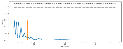
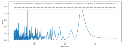
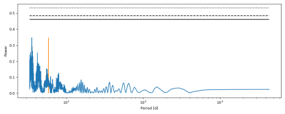
Figure 8: Periodogram of the RV residuals to models 6 (top) and 5 (middle) for the full RV dataset, and of the RV residuals to model 6 for the HARPS data alone (bottom). The vertical line indicates the period of the planetary candidate TOI-201.02. There are no significant signals in any of the periodograms.

Although we cannot detect TOI-201.02 in the RV data, we can still use this data to estimate its maximum mass. For this, we ran a more constrained two-planet model on the FEROS and HARPS data, fixing the periods and epochs to those listed in ExoFOP-TESS. We also fixed the eccentricity of the inner planet to zero, since we can expect its orbit to be circularized by its proximity to the host star. Using the semi-amplitude of the resulting Keplerian fit, $K=1.76^{+1.84}_{-1.14}\,m/s$, we estimate a maximum mass for TOI-201.02 of $M_{max}\approx 37.5\,M_{\oplus}$ with 98% confidence.

3.3 Joint transit and radial velocity model

Having shown that TOI-201 b can be detected in the radial velocities alone, we perform a joint modelling of the full set of radial velocities and transit data. We adopt a one-planet model, with $\mathrm{e\sin{\omega}}$ and $\mathrm{e\cos{\omega}}$ constrained using the posteriors from model 6. We also include two separate GPs: one on the joint FEROS, HARPS, CORALIE, and Minerva-Australis radial velocities, to account for the stellar activity, as done in model 6; and one on the TESS light curve, to account for instrumental effects such as the over-estimation of flux for the partial transit in Sector 8 (Fig. 1, bottom panel). Rather than fit for the planet-to-star radius ratio and impact parameter of the orbit directly, we adopt the ($\mathrm{r_{1},\,r_{2}}$) parametrization of Espinoza (2018), which allows for efficient sampling with uniform priors.

We find a log-evidence of $\ln(Z)=1236042.914\pm 0.008$. The priors are listed in Table 4, and the posteriors in Table 5. Figure 9 shows the phase-folded data and the full model for the light curves and radial velocities. Using the stellar parameters obtained in 3.1, and the posterior distributions of the full model, we compute a mass of $\mathrm{0.42^{+0.05}_{-0.03}\,M_{J}}$ and a radius of $\mathrm{1.008^{+0.012}_{-0.015}\,R_{J}}$ for TOI-201 b. The physical parameters, and derived orbital parameters, are also listed in Table 5.

The Minerva-Australis radial velocities have larger error bars and show more dispersion from the fitted model than those of the other three RV datasets, as can be clearly seen in Fig. 9 (b, bottom panel). Therefore, we also tested an analogous model in which the Minerva-Australis RVs were not included. The resulting parameters are the same within uncertainties, and the uncertainties on the parameters are similar for both models. This being the case, we prefer the model including the Minerva-Australis RVs.

Table 4: Prior parameter distributions for the joint transit and RV analysis. $\mathcal{U}(a,b)$ indicates a uniform distribution between $a$ and $b$; $\mathcal{N}(a,b)$ a normal distribution with mean $a$ and standard deviation $b$; $\mathcal{J}(a,b)$ a Jeffreys or log-uniform distribution between $a$ and $b$.

Parameter	Distribution
$\mu_{\mathrm{{HARPS}}}$ [km/s]	$\mathcal{U}(16.85,16.96)$
$\mu_{\mathrm{{FEROS}}}$ [km/s]	$\mathcal{U}(16.82,16.93)$
$\mu_{\mathrm{{CORALIE}}}$ [km/s]	$\mathcal{U}(-30,30)$
$\mu_{\mathrm{{MINERVA}}}$ [km/s]	$\mathcal{U}(-30,30)$
$\sigma_{\mathrm{{HARPS}}}$ [km/s]	$\mathcal{J}(0.011,0.013)$
$\sigma_{\mathrm{{FEROS}}}$ [km/s]	$\mathcal{J}(0.011,0.015)$
$\sigma_{\mathrm{{CORALIE}}}$ [km/s]	$\mathcal{J}(0.001,100)$
$\sigma_{\mathrm{{MINERVA}}}$ [km/s]	$\mathcal{J}(0.001,100)$
Pb [d]	$\mathcal{N}(52.978306,0.1)$
T0b [d]	$\mathcal{N}(2458376.052124,0.1)$
Kb [km/s]	$\mathcal{U}(0.011,0.021)$
$e\sin{\omega}_{\mathrm{b}}$	$\mathcal{U}(0.01,0.36)$
$e\cos{\omega}_{\mathrm{b}}$	$\mathcal{U}(-0.30,0.09)$
$\sigma_{\mathrm{{GP,RV}}}$	$\mathcal{J}(0.01,100)$
$\rho_{\mathrm{{GP,RV}}}$	$\mathcal{J}(0.01,100)$
r1,b	$\mathcal{U}(0,1)$
r2,b	$\mathcal{U}(0,1)$
$\rho$	$\mathcal{J}(100.,10000.)$
q1,TESS	$\mathcal{U}(0,1)$
q2,TESS	$\mathcal{U}(0,1)$
$m_{\mathrm{{d,TESS}}}$	1.0 (fixed)
$m_{\mathrm{{flux,TESS}}}$	$\mathcal{N}(0,0.1)$
$\sigma_{\mathrm{{TESS}}}$	$\mathcal{J}(0.1,1000)$
$\sigma_{\mathrm{{GP,TESS}}}$	$\mathcal{J}(1\times 10^{-6},1000000)$
$\rho_{\mathrm{{GP,TESS}}}$	$\mathcal{J}(0.001,1000)$
q1,NGTS	$\mathcal{U}(0,1)$
q2,NGTS	$\mathcal{U}(0,1)$
$m_{\mathrm{{d,NGTS}}}$	1.0 (fixed)
$m_{\mathrm{{flux,NGTS}}}$	$\mathcal{N}(0,0.1)$
$\sigma_{\mathrm{{NGTS}}}$	$\mathcal{J}(0.1,1000)$

Table 5: Parameters for planet TOI-201 b. Top: Posterior parameter distributions for the joint transit and RV analysis. Bottom: derived orbital parameters and physical parameters.

Parameter	Distribution
$\mu_{\mathrm{{HARPS}}}$ [km/s]	$16.92^{+0.01}_{-0.01}$
$\mu_{\mathrm{{FEROS}}}$ [km/s]	$16.89^{+0.01}_{-0.01}$
$\mu_{\mathrm{{CORALIE}}}$ [km/s]	$16.87^{+0.02}_{-0.01}$
$\mu_{\mathrm{{MINERVA}}}$ [km/s]	$0.02^{+0.01}_{-0.01}$
$\sigma_{\mathrm{{HARPS}}}$ [km/s]	$0.0117^{+0.0008}_{-0.0005}$
$\sigma_{\mathrm{{FEROS}}}$ [km/s]	$0.014^{+0.001}_{-0.001}$
$\sigma_{\mathrm{{CORALIE}}}$ [km/s]	$0.019^{+0.009}_{-0.007}$
$\sigma_{\mathrm{{MINERVA}}}$ [km/s]	$0.026^{+0.004}_{-0.004}$
Pb [d]	$52.97818^{+0.00004}_{-0.00004}$
T0b [BJD]	$2458376.0520^{+0.0003}_{-0.0003}$
Kb [km/s]	$0.019^{+0.001}_{-0.002}$
$e\sin{\omega}_{\mathrm{b}}$	$0.28^{+0.06}_{-0.09}$
$e\cos{\omega}_{\mathrm{b}}$	$0.04^{+0.04}_{-0.07}$
$\sigma_{\mathrm{{GP}}}$	$0.025^{+0.008}_{-0.006}$
$\rho_{\mathrm{{GP}}}$	$70^{+21}_{-27}$
r1,b	$0.82^{+0.01}_{-0.01}$
r2,b	$0.0786^{+0.0010}_{-0.0007}$
$\rho$	$854^{+288}_{-154}$
q1,TESS	$0.22^{+0.06}_{-0.06}$
q2,TESS	$0.25^{+0.33}_{-0.18}$
$m_{\mathrm{{d,TESS}}}$	1.0
$m_{\mathrm{{flux,TESS}}}$	$-0.00002^{+0.00002}_{-0.00002}$
$\sigma_{\mathrm{{TESS}}}$	$73^{+5}_{-5}$
$\sigma_{\mathrm{{GP,TESS}}}$	$0.00030^{+0.00001}_{-0.00001}$
$\rho_{\mathrm{{GP,TESS}}}$	$0.64^{+0.03}_{-0.03}$
q1,NGTS	$0.47^{+0.23}_{-0.19}$
q2,NGTS	$0.38^{+0.32}_{-0.25}$
$m_{\mathrm{{d,NGTS}}}$	1.0
$m_{\mathrm{{flux,NGTS}}}$	$0.0001^{+0.0002}_{-0.0002}$
$\sigma_{\mathrm{{NGTS}}}$	$5^{+56}_{-4}$
$e_{\mathrm{b}}$	$0.28^{+0.06}_{-0.09}$
$\omega_{\mathrm{b}}$ [deg]	$82^{+14}_{-9}$
$a$ [AU]	$0.30^{+0.02}_{-0.03}$
$\mathrm{M_{b}}$ [MJ]	$0.42^{+0.05}_{-0.03}$
$\mathrm{R_{b}}$ [RJ]	$1.008^{+0.012}_{-0.015}$
$T_{\mathrm{eq}}$ [K]	$759^{+37}_{-26}$

Figure 9: Joint transit and RV model. (a): Left panel: phase-folded TESS data (blue points), binned TESS data (white points) and model (black line). Centre panel: as left, for NGTS data. Right panel: phase-folded FEROS, HARPS, CORALIE, and Minerva-Australis radial velocities, with the RV GP component removed, and Keplerian model component (black line). (b): Top: Radial velocity data for FEROS, HARPS, CORALIE, and Minerva-Australis, full model, and Keplerian and GP components. Bottom: RV residuals. (c): TESS data and full model for Sectors 1-13 (left panel) and 27-28 (right panel).

4 Discussion and Conclusions

We have presented the confirmation through radial velocities of the transiting planet TOI-201 b. In addition to the RV signal due to TOI-201 b, we also see long-period signals in both the radial velocities and in the H_α and log($R^{\prime}_{HK}$) activity indicators. We therefore conclude that the long-period variations in RV are likely due to stellar activity, and model them using a Gaussian process.

We are unable to confirm the second planetary candidate around this star, TOI-201.02. Two-planet fits to the radial velocities are not favoured by likelihood comparison, and there are no signals at $\sim 5.8$ d in the RV residuals to the one-planet fit. Likewise, we were not able to retrieve a Keplerian, modelled using the candidate’s period and estimated mass, that we injected into the randomly shuffled residuals of the one-planet model.

TOI-201 b is an eccentric warm giant, orbiting a young F-type star. More specifically, TOI-201 falls within the youngest 5% of exoplanet host stars with measured ages, making this system a valuable addition to the known planets around young stars, which are important for testing and constraining planet formation and evolution theories (e.g. Baraffe et al., 2008; Mordasini et al., 2012b, a). At $\lesssim 1\,\mathrm{Gyr}$, some evolutionary processes that are typically not observable are still ongoing, such as photoevaporation of planetary envelopes (David et al., 2020) for small planets. Likewise, giant planet formation theory has difficulties fixing the luminosity of a cooling planet as a function of time (”hot start” vs. ”cool start” models, e.g. Mordasini et al. 2012b), and representatives of giant planets that are currently cooling may help to constrain that. TOI-201 b also joins the small but growing population of longer-period giant planets, helping to populate a still relatively sparse region of the radius-period diagram (Figure 10). On this diagram, it is located closest to Kepler-117 c (period $\mathrm{50.790391\pm 0.000014\,d}$, radius $\mathrm{1.101\pm 0.035\,R_{J}}$, mass $\mathrm{1.84\pm 0.18\,M_{J}}$, eccentricity $\mathrm{0.0323\pm 0.0033}$, from Bruno et al. 2015) and Kepler-30 c (period $\mathrm{60.32503\pm 0.00010\,d}$, radius $\mathrm{1.069\pm 0.025\,R_{J}}$, mass $\mathrm{1.686\pm 0.016\,M_{J}}$, eccentricity $\mathrm{0.0115\pm 0.0005}$, from Panichi et al. 2018) but is noticeably less massive and dense, and more eccentric, than both these planets. Given the relative youth of the TOI-201 system, with a stellar age of $\mathrm{0.87^{+0.46}_{-0.49}\,Gyr}$ (for comparison, Bruno et al. 2015 find an age of $\mathrm{5.3\pm 1.4\,Gyr}$ for Kepler-117), the difference in density may be partly explained by a still-contracting TOI-201 b.

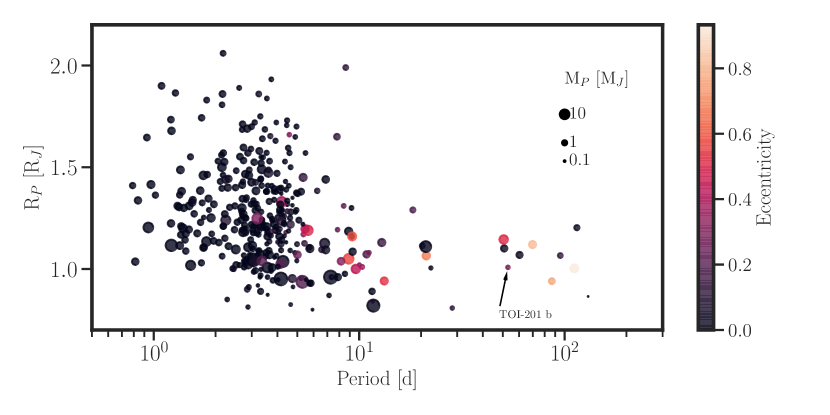
Figure 10: Radius-period diagram for giant planets ($\mathrm{R_{p}\geq 0.8R_{J}}$), with masses and radii measured to better than 25%, obtained from the TEPCAT catalogue (Southworth, 2011). The markers are scaled by planet mass and colour-coded by eccentricity. TOI-201 b is labelled.

As noted in the introduction, the size and mass of warm Jupiters is determined by their metallicity. We use the structure models of Thorngren & Fortney (2019) to constrain the heavy element mass for TOI-201 b. Using the planet mass and insolation flux, and the stellar age, we employ a retrieval algorithm to recover the metallicity which would match the observed radius. The metallicity required to explain the planet’s radius is strongly correlated with the age, indicating that it appears to still be cooling - and therefore contracting - fairly rapidly. The bulk metallicity we obtain is $Z_{p}=0.16^{+0.03}_{-0.02}$, which is moderately low for the planet’s mass compared to similarly massive planets from Thorngren & Fortney (2019), but still within the range of values obtained in that work. Given the high precision on the planetary parameters, modelling uncertainty (e.g. in the equation of state) is probably larger than the statistical uncertainty from the parameters. We estimate this at around a 20% relative uncertainty, though recent work by Müller et al. (2020) cautions that the interplay between various model assumptions (particularly in the choice of equations of state, the distribution of heavy elements, and the modelling of its effect on the opacity) may mean it is higher. The posterior distribution of the parameters is shown in Fig. 11.

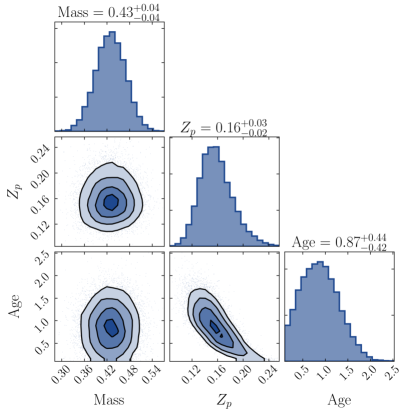
Figure 11: Posterior distribution of heavy elements, age, and mass, from the structure models of Thorngren & Fortney (2019).

The Rossiter-McLaughlin effect (Rossiter, 1924; McLaughlin, 1924) allows the stellar obliquity to be measured. These measurements are useful for constraining migration scenarios, and are particularly valuable for planets such as TOI-201 b, which are located at longer orbital distances where tidal realignment is no longer in play (see e.g. Triaud 2018 for a review). It is worth noting that all the RV measurements used in the analysis in Section 3 fall outside the transit, and so are not affected by the Rossiter-McLaughlin effect. For TOI-201 b, the expected semi-amplitude of the Rossiter-McLaughlin signal is of $\mathrm{\approx 40m/s}$ for an aligned orbit (using the equation of Winn 2010), making this system a good candidate for such observations.

Appendix A Radial velocity and activity indices

In this appendix, we present the radial velocities and activity indices, where applicable. Table 6 shows the data for FEROS, and Table 7 the data for HARPS, both computed using the CERES pipeline. Table 8 shows the radial velocities obtained from the CORALIE spectra. Table 9 shows the radial velocities obtained from the Minerva-Australis spectra.

Table 6: RV and activity indices obtained from the FEROS spectra.

BJD - 2457000 [d]	RV [km/s]	Bisector	FWHM	SNR	Hα	log($R^{\prime}_{HK}$)	Na II	He I
$2458449.72902056$	$16.8300\pm 0.0082$	$0.036\pm 0.007$	$15.5668$	$193$	$0.1075\pm 0.0009$	$-4.749\pm 0.026$	$0.3978\pm 0.0020$	$0.4992\pm 0.0025$
$2458449.82501961$	$16.8526\pm 0.0090$	$0.031\pm 0.007$	$15.6119$	$168$	$0.1076\pm 0.0010$	$-4.726\pm 0.026$	$0.3912\pm 0.0022$	$0.5022\pm 0.0028$
$2458449.81907519$	$16.8447\pm 0.0086$	$0.008\pm 0.007$	$15.6457$	$182$	$0.1065\pm 0.0009$	$-4.741\pm 0.027$	$0.3910\pm 0.0021$	$0.5019\pm 0.0026$
$2458450.78211913$	$16.8616\pm 0.0084$	$0.011\pm 0.007$	$15.6056$	$187$	$0.1070\pm 0.0009$	$-4.757\pm 0.027$	$0.3982\pm 0.0020$	$0.5033\pm 0.0026$
$2458450.77751112$	$16.8614\pm 0.0083$	$0.027\pm 0.007$	$15.6184$	$191$	$0.1064\pm 0.0009$	$-4.739\pm 0.026$	$0.3979\pm 0.0020$	$0.5012\pm 0.0026$
$2458451.80088761$	$16.8751\pm 0.0087$	$0.018\pm 0.007$	$15.6244$	$179$	$0.1087\pm 0.0010$	$-4.705\pm 0.025$	$0.3923\pm 0.0021$	$0.5011\pm 0.0027$
$2458451.80550488$	$16.8632\pm 0.0087$	$0.025\pm 0.007$	$15.6687$	$177$	$0.1090\pm 0.0010$	$-4.756\pm 0.027$	$0.3908\pm 0.0021$	$0.4983\pm 0.0027$
$2458452.81008207$	$16.8672\pm 0.0093$	$0.038\pm 0.008$	$15.6380$	$161$	$0.1093\pm 0.0011$	$-4.714\pm 0.026$	$0.4017\pm 0.0024$	$0.4986\pm 0.0030$
$2458467.81642493$	$16.8789\pm 0.0088$	$0.036\pm 0.007$	$15.5752$	$174$	$0.1081\pm 0.0010$	$-4.715\pm 0.026$	$0.3830\pm 0.0022$	$0.4967\pm 0.0026$
$2458468.80955367$	$16.8986\pm 0.0116$	$0.048\pm 0.009$	$15.6108$	$115$	$0.1101\pm 0.0016$	$-4.771\pm 0.033$	$0.3838\pm 0.0035$	$0.5044\pm 0.0041$
$2458469.81379926$	$16.8014\pm 0.0086$	$0.026\pm 0.007$	$15.7449$	$184$	$0.1051\pm 0.0010$	$-4.764\pm 0.028$	$0.3908\pm 0.0021$	$0.5026\pm 0.0026$
$2458483.80487685$	$16.8562\pm 0.0088$	$0.015\pm 0.007$	$15.6195$	$174$	$0.1103\pm 0.0010$	$-4.734\pm 0.027$	$0.3971\pm 0.0022$	$0.5024\pm 0.0028$
$2458484.68236998$	$16.8389\pm 0.0098$	$0.029\pm 0.008$	$15.6311$	$147$	$0.1139\pm 0.0012$	$-4.728\pm 0.028$	$0.3916\pm 0.0025$	$0.4989\pm 0.0032$
$2458493.74536456$	$16.8351\pm 0.0096$	$0.030\pm 0.008$	$15.6102$	$152$	$0.1136\pm 0.0012$	$-4.770\pm 0.030$	$0.3987\pm 0.0025$	$0.4949\pm 0.0032$
$2458502.71190832$	$16.8165\pm 0.0103$	$0.045\pm 0.008$	$15.6693$	$136$	$0.1140\pm 0.0014$	$-4.760\pm 0.029$	$0.3852\pm 0.0029$	$0.4974\pm 0.0035$
$2458503.66565834$	$16.8097\pm 0.0086$	$0.041\pm 0.007$	$15.6483$	$179$	$0.1081\pm 0.0010$	$-4.775\pm 0.028$	$0.3916\pm 0.0021$	$0.4952\pm 0.0025$
$2458521.58681966$	$16.8295\pm 0.0087$	$0.030\pm 0.007$	$15.5953$	$176$	$0.1123\pm 0.0010$	$-4.737\pm 0.026$	$0.3975\pm 0.0021$	$0.4946\pm 0.0027$
$2458542.59373287$	$16.8271\pm 0.0090$	$0.031\pm 0.007$	$15.6742$	$170$	$0.1095\pm 0.0010$	$-4.762\pm 0.028$	$0.3817\pm 0.0022$	$0.4945\pm 0.0027$
$2458543.57904173$	$16.8330\pm 0.0083$	$0.024\pm 0.007$	$15.6701$	$191$	$0.1076\pm 0.0009$	$-4.760\pm 0.027$	$0.3774\pm 0.0020$	$0.4961\pm 0.0024$
$2458544.66708564$	$16.8440\pm 0.0089$	$0.008\pm 0.007$	$15.7129$	$171$	$0.1067\pm 0.0010$	$-4.804\pm 0.034$	$0.3864\pm 0.0022$	$0.4961\pm 0.0028$
$2458545.62781982$	$16.8214\pm 0.0101$	$0.031\pm 0.008$	$15.6486$	$141$	$0.1071\pm 0.0013$	$-4.792\pm 0.033$	$0.3856\pm 0.0028$	$0.4884\pm 0.0035$
$2458546.64551855$	$16.8438\pm 0.0106$	$0.043\pm 0.008$	$15.7462$	$132$	$0.1109\pm 0.0014$	$-4.804\pm 0.036$	$0.3896\pm 0.0029$	$0.4950\pm 0.0036$
$2458547.57166286$	$16.8337\pm 0.0101$	$0.023\pm 0.008$	$15.6793$	$141$	$0.1092\pm 0.0013$	$-4.794\pm 0.032$	$0.3938\pm 0.0028$	$0.4926\pm 0.0034$
$2458548.62966483$	$16.8329\pm 0.0087$	$0.017\pm 0.007$	$15.7019$	$179$	$0.1068\pm 0.0010$	$-4.777\pm 0.029$	$0.3909\pm 0.0022$	$0.4973\pm 0.0028$
$2458550.64407369$	$16.8320\pm 0.0085$	$0.023\pm 0.007$	$15.6949$	$184$	$0.1087\pm 0.0010$	$-4.816\pm 0.033$	$0.3901\pm 0.0021$	$0.4930\pm 0.0027$
$2458554.63465672$	$16.8501\pm 0.0103$	$0.019\pm 0.008$	$15.7519$	$138$	$0.1140\pm 0.0014$	$-4.781\pm 0.033$	$0.4019\pm 0.0028$	$0.4969\pm 0.0035$
$2458555.62085265$	$16.8363\pm 0.0087$	$0.026\pm 0.007$	$15.7304$	$177$	$0.1089\pm 0.0010$	$-4.767\pm 0.029$	$0.4028\pm 0.0022$	$0.4978\pm 0.0027$
$2458556.65947799$	$16.8486\pm 0.0111$	$0.001\pm 0.009$	$15.7611$	$124$	$0.1107\pm 0.0015$	$-4.797\pm 0.041$	$0.4070\pm 0.0032$	$0.4969\pm 0.0037$
$2458558.59692547$	$16.8513\pm 0.0113$	$0.035\pm 0.009$	$15.7526$	$121$	$0.1134\pm 0.0016$	$-4.791\pm 0.034$	$0.4061\pm 0.0032$	$0.4972\pm 0.0038$
$2458560.65048512$	$16.8578\pm 0.0097$	$0.020\pm 0.008$	$15.8235$	$152$	$0.1092\pm 0.0013$	$-4.782\pm 0.036$	$0.3930\pm 0.0027$	$0.4934\pm 0.0031$
$2458566.60098112$	$16.8672\pm 0.0084$	$0.026\pm 0.007$	$15.7052$	$187$	$0.1078\pm 0.0009$	$-4.763\pm 0.030$	$0.3895\pm 0.0021$	$0.4959\pm 0.0025$
$2458568.56334852$	$16.8670\pm 0.0087$	$0.038\pm 0.007$	$15.6716$	$177$	$0.1098\pm 0.0010$	$-4.749\pm 0.028$	$0.3948\pm 0.0022$	$0.4946\pm 0.0026$
$2458569.55147254$	$16.8569\pm 0.0090$	$0.039\pm 0.007$	$15.6554$	$168$	$0.1100\pm 0.0011$	$-4.780\pm 0.030$	$0.3890\pm 0.0023$	$0.4970\pm 0.0028$
$2458570.59258685$	$16.8796\pm 0.0106$	$0.001\pm 0.008$	$15.6557$	$132$	$0.1094\pm 0.0014$	$-4.789\pm 0.035$	$0.3898\pm 0.0030$	$0.4984\pm 0.0035$
$2458572.59221071$	$16.8804\pm 0.0099$	$0.029\pm 0.008$	$15.7094$	$146$	$0.1083\pm 0.0013$	$-4.746\pm 0.031$	$0.3868\pm 0.0027$	$0.5050\pm 0.0034$
$2458595.50775173$	$16.8567\pm 0.0137$	$0.026\pm 0.010$	$15.5962$	$93$	$0.1176\pm 0.0020$	$-4.822\pm 0.046$	$0.3869\pm 0.0043$	$0.4957\pm 0.0052$
$2458597.49996378$	$16.8591\pm 0.0101$	$0.008\pm 0.008$	$15.6091$	$143$	$0.1135\pm 0.0013$	$-4.762\pm 0.031$	$0.3817\pm 0.0027$	$0.4962\pm 0.0033$
$2458617.50211498$	$16.8542\pm 0.0093$	$0.022\pm 0.008$	$15.7453$	$161$	$0.1088\pm 0.0011$	$-4.790\pm 0.044$	$0.4038\pm 0.0024$	$0.4957\pm 0.0030$
$2458670.93647358$	$16.9094\pm 0.0109$	$0.025\pm 0.009$	$15.6949$	$126$	$0.1051\pm 0.0014$	$-4.739\pm 0.054$	$0.3878\pm 0.0030$	$0.4915\pm 0.0036$
$2458718.87031042$	$16.9107\pm 0.0091$	$0.012\pm 0.007$	$15.6143$	$165$	$0.1108\pm 0.0011$	$-4.748\pm 0.028$	$0.3934\pm 0.0024$	$0.4885\pm 0.0029$
$2458721.92050686$	$16.9072\pm 0.0110$	$0.016\pm 0.009$	$15.6205$	$124$	$0.1099\pm 0.0014$	$-4.706\pm 0.028$	$0.3911\pm 0.0032$	$0.4924\pm 0.0038$
$2458723.89624752$	$16.9272\pm 0.0098$	$0.015\pm 0.008$	$15.6508$	$147$	$0.1089\pm 0.0012$	$-4.748\pm 0.029$	$0.3958\pm 0.0026$	$0.4913\pm 0.0032$
$2458724.92469963$	$16.9254\pm 0.0120$	$0.024\pm 0.009$	$15.6280$	$111$	$0.1102\pm 0.0016$	$-4.724\pm 0.031$	$0.3926\pm 0.0035$	$0.4925\pm 0.0043$
$2458784.85036502$	$16.9450\pm 0.0098$	$0.013\pm 0.008$	$15.5626$	$147$	$0.1071\pm 0.0012$	$-4.783\pm 0.030$	$0.3894\pm 0.0026$	$0.4911\pm 0.0032$
$2458792.78919017$	$16.9334\pm 0.0089$	$0.019\pm 0.007$	$15.6070$	$171$	$0.1054\pm 0.0010$	$-4.770\pm 0.028$	$0.3861\pm 0.0023$	$0.4970\pm 0.0028$
$2458795.78669357$	$16.9561\pm 0.0089$	$0.023\pm 0.007$	$15.5507$	$170$	$0.1059\pm 0.0010$	$-4.762\pm 0.028$	$0.3883\pm 0.0023$	$0.4904\pm 0.0027$
$2458800.72101439$	$16.9028\pm 0.0096$	$0.019\pm 0.008$	$15.5996$	$150$	$0.1079\pm 0.0012$	$-4.789\pm 0.031$	$0.3859\pm 0.0026$	$0.4981\pm 0.0031$
$2458802.84973114$	$16.8795\pm 0.0089$	$0.025\pm 0.007$	$15.5810$	$171$	$0.1075\pm 0.0010$	$-4.734\pm 0.026$	$0.3854\pm 0.0023$	$0.5027\pm 0.0027$
$2458804.71328670$	$16.8841\pm 0.0091$	$0.038\pm 0.007$	$15.6398$	$165$	$0.1067\pm 0.0011$	$-4.762\pm 0.028$	$0.3886\pm 0.0023$	$0.4982\pm 0.0028$
$2458806.69577168$	$16.8941\pm 0.0085$	$0.019\pm 0.007$	$15.6158$	$182$	$0.1052\pm 0.0010$	$-4.749\pm 0.027$	$0.3894\pm 0.0022$	$0.5048\pm 0.0026$
$2458911.59453852$	$16.8965\pm 0.0099$	$0.028\pm 0.008$	$15.7209$	$147$	$0.1047\pm 0.0012$	$-4.743\pm 0.028$	$0.3857\pm 0.0027$	$0.4960\pm 0.0034$
$2458917.63877563$	$16.8883\pm 0.0204$	$0.021\pm 0.013$	$15.7356$	$59$	$0.1110\pm 0.0032$	$-4.732\pm 0.064$	$0.3940\pm 0.0069$	$0.5077\pm 0.0082$

Table 7: RV and activity indices obtained from the HARPS spectra.

BJD - 2457000 [d]	RV [km/s]	Bisector	FWHM	SNR	Hα	log($R^{\prime}_{HK}$)	Na II	He I
$1464.83460002$	$16.8822\pm 0.0035$	$0.015\pm 0.003$	$14.3788$	$83$	$0.1084\pm 0.0008$	$-4.771\pm 0.029$	$0.4144\pm 0.0016$	$0.4977\pm 0.0019$
$1464.82626718$	$16.8868\pm 0.0035$	$0.017\pm 0.003$	$14.3902$	$83$	$0.1071\pm 0.0008$	$-4.763\pm 0.029$	$0.4139\pm 0.0016$	$0.4976\pm 0.0019$
$1465.80299404$	$16.9102\pm 0.0020$	$0.028\pm 0.002$	$14.3445$	$118$	$0.1080\pm 0.0005$	$-4.714\pm 0.025$	$0.4111\pm 0.0011$	$0.4978\pm 0.0013$
$1465.79547085$	$16.9147\pm 0.0020$	$0.025\pm 0.002$	$14.3513$	$120$	$0.1077\pm 0.0005$	$-4.707\pm 0.025$	$0.4093\pm 0.0011$	$0.4973\pm 0.0013$
$1466.78878939$	$16.9063\pm 0.0022$	$0.006\pm 0.002$	$14.4190$	$99$	$0.1079\pm 0.0006$	$-4.701\pm 0.025$	$0.4108\pm 0.0013$	$0.4956\pm 0.0015$
$1466.79644105$	$16.9112\pm 0.0020$	$0.019\pm 0.002$	$14.4287$	$107$	$0.1074\pm 0.0006$	$-4.675\pm 0.024$	$0.4131\pm 0.0012$	$0.4949\pm 0.0014$
$1481.74528823$	$16.8882\pm 0.0020$	$0.024\pm 0.002$	$14.3635$	$120$	$0.1061\pm 0.0006$	$-4.727\pm 0.026$	$0.4170\pm 0.0012$	$0.4979\pm 0.0013$
$1482.75123537$	$16.8830\pm 0.0020$	$0.020\pm 0.002$	$14.3771$	$142$	$0.1062\pm 0.0004$	$-4.722\pm 0.025$	$0.4160\pm 0.0009$	$0.4982\pm 0.0011$
$1482.74376858$	$16.8829\pm 0.0020$	$0.020\pm 0.002$	$14.3770$	$145$	$0.1057\pm 0.0004$	$-4.740\pm 0.026$	$0.4159\pm 0.0009$	$0.4965\pm 0.0011$
$1483.77055220$	$16.8847\pm 0.0020$	$0.009\pm 0.002$	$14.3640$	$121$	$0.1066\pm 0.0005$	$-4.736\pm 0.026$	$0.4138\pm 0.0011$	$0.4978\pm 0.0013$
$1483.76263412$	$16.8846\pm 0.0020$	$0.014\pm 0.002$	$14.3626$	$118$	$0.1067\pm 0.0005$	$-4.747\pm 0.027$	$0.4135\pm 0.0011$	$0.4975\pm 0.0013$
$1576.54303679$	$16.9129\pm 0.0029$	$0.036\pm 0.002$	$14.3866$	$90$	$0.1044\pm 0.0008$	$-4.894\pm 0.037$	$0.4165\pm 0.0015$	$0.4960\pm 0.0018$
$1762.82961396$	$16.9229\pm 0.0020$	$0.014\pm 0.002$	$14.4052$	$113$	$0.1070\pm 0.0006$	$-4.721\pm 0.026$	$0.4196\pm 0.0012$	$0.4996\pm 0.0014$
$1763.79774196$	$16.8988\pm 0.0020$	$0.030\pm 0.002$	$14.3579$	$114$	$0.1061\pm 0.0006$	$-4.720\pm 0.025$	$0.4225\pm 0.0012$	$0.5017\pm 0.0014$
$1764.83063596$	$16.9055\pm 0.0020$	$0.025\pm 0.002$	$14.3443$	$139$	$0.1050\pm 0.0005$	$-4.751\pm 0.027$	$0.4237\pm 0.0010$	$0.5010\pm 0.0012$
$1773.87633433$	$16.9275\pm 0.0020$	$0.014\pm 0.002$	$14.3624$	$109$	$0.1054\pm 0.0006$	$-4.782\pm 0.029$	$0.4233\pm 0.0013$	$0.4989\pm 0.0014$
$1775.86482034$	$16.9506\pm 0.0040$	$0.004\pm 0.003$	$14.3949$	$78$	$0.1056\pm 0.0009$	$-4.784\pm 0.030$	$0.4177\pm 0.0017$	$0.4979\pm 0.0020$
$1777.74548666$	$16.9247\pm 0.0083$	$0.015\pm 0.006$	$14.3560$	$52$	$0.1058\pm 0.0015$	$-5.023\pm 0.060$	$0.4254\pm 0.0028$	$0.4988\pm 0.0031$
$1803.76107908$	$16.9097\pm 0.0020$	$0.032\pm 0.002$	$14.4174$	$111$	$0.1064\pm 0.0006$	$-4.757\pm 0.027$	$0.4212\pm 0.0012$	$0.5007\pm 0.0014$
$1810.87660156$	$16.8759\pm 0.0020$	$0.012\pm 0.002$	$14.4132$	$109$	$0.1054\pm 0.0006$	$-4.771\pm 0.028$	$0.4212\pm 0.0012$	$0.5010\pm 0.0014$
$1820.86191239$	$16.9179\pm 0.0020$	$0.015\pm 0.002$	$14.3700$	$114$	$0.1052\pm 0.0006$	$-4.766\pm 0.028$	$0.4167\pm 0.0012$	$0.5006\pm 0.0013$
$1831.79439764$	$16.9347\pm 0.0020$	$0.029\pm 0.002$	$14.3699$	$121$	$0.1043\pm 0.0006$	$-4.761\pm 0.028$	$0.4115\pm 0.0011$	$0.4982\pm 0.0012$
$1833.69330017$	$16.9464\pm 0.0030$	$0.023\pm 0.002$	$14.3629$	$88$	$0.1040\pm 0.0008$	$-4.776\pm 0.029$	$0.4138\pm 0.0015$	$0.5002\pm 0.0018$
$1836.70976685$	$16.9510\pm 0.0020$	$0.022\pm 0.002$	$14.3267$	$107$	$0.1058\pm 0.0007$	$-4.757\pm 0.027$	$0.4183\pm 0.0013$	$0.4990\pm 0.0015$
$1839.73047160$	$16.9502\pm 0.0021$	$0.021\pm 0.002$	$14.3294$	$100$	$0.1038\pm 0.0007$	$-4.776\pm 0.029$	$0.4232\pm 0.0014$	$0.4998\pm 0.0016$
$1848.70736633$	$16.9491\pm 0.0020$	$0.042\pm 0.002$	$14.3724$	$152$	$0.1045\pm 0.0004$	$-4.760\pm 0.027$	$0.4180\pm 0.0009$	$0.4977\pm 0.0010$
$1853.82221087$	$16.9462\pm 0.0020$	$0.018\pm 0.002$	$14.3981$	$106$	$0.1044\pm 0.0006$	$-4.748\pm 0.028$	$0.4055\pm 0.0012$	$0.4949\pm 0.0014$
$1855.62240768$	$16.9285\pm 0.0020$	$0.011\pm 0.002$	$14.3667$	$113$	$0.1045\pm 0.0006$	$-4.758\pm 0.027$	$0.4148\pm 0.0012$	$0.4974\pm 0.0014$
$1866.53795150$	$16.9294\pm 0.0336$	$0.043\pm 0.025$	$14.2712$	$17$	$0.0828\pm 0.0058$	$\cdots$	$0.4236\pm 0.0095$	$0.4839\pm 0.0090$
$1866.55739621$	$16.9209\pm 0.0023$	$0.029\pm 0.002$	$14.3386$	$97$	$0.1031\pm 0.0007$	$-4.759\pm 0.028$	$0.4061\pm 0.0014$	$0.4969\pm 0.0016$
$1868.53027483$	$16.9340\pm 0.0020$	$0.016\pm 0.002$	$14.3383$	$116$	$0.1048\pm 0.0006$	$-4.761\pm 0.027$	$0.4005\pm 0.0011$	$0.4917\pm 0.0013$
$1875.52489656$	$16.9384\pm 0.0020$	$0.020\pm 0.002$	$14.3597$	$132$	$0.1041\pm 0.0005$	$-4.752\pm 0.027$	$0.4081\pm 0.0010$	$0.4947\pm 0.0011$
$1877.62220328$	$16.9245\pm 0.0049$	$0.028\pm 0.004$	$14.3702$	$71$	$0.1015\pm 0.0009$	$-4.786\pm 0.030$	$0.4067\pm 0.0017$	$0.4981\pm 0.0021$
$1884.61075979$	$16.9418\pm 0.0056$	$0.030\pm 0.004$	$14.3274$	$66$	$0.1051\pm 0.0010$	$-4.792\pm 0.031$	$0.4170\pm 0.0020$	$0.4988\pm 0.0023$
$1886.65333879$	$16.9538\pm 0.0031$	$0.027\pm 0.002$	$14.3517$	$87$	$0.1047\pm 0.0007$	$-4.824\pm 0.032$	$0.4172\pm 0.0015$	$0.5010\pm 0.0017$
$1889.64841759$	$16.9595\pm 0.0033$	$0.028\pm 0.002$	$14.3437$	$85$	$0.1050\pm 0.0007$	$-4.808\pm 0.031$	$0.4221\pm 0.0015$	$0.4991\pm 0.0018$
$1893.71018832$	$16.9813\pm 0.0020$	$0.020\pm 0.002$	$14.3765$	$104$	$0.1049\pm 0.0005$	$-4.804\pm 0.031$	$0.4128\pm 0.0012$	$0.4977\pm 0.0013$
$1896.53584191$	$16.9733\pm 0.0038$	$0.024\pm 0.003$	$14.3444$	$80$	$0.1049\pm 0.0008$	$-4.810\pm 0.031$	$0.4067\pm 0.0016$	$0.4951\pm 0.0018$
$1901.52855834$	$16.9797\pm 0.0020$	$0.012\pm 0.002$	$14.3447$	$120$	$0.1043\pm 0.0005$	$-4.744\pm 0.027$	$0.4150\pm 0.0011$	$0.4980\pm 0.0013$

Table 8: RV obtained from the CORALIE spectra.

BJD - 2457000 [d]	RV [km/s]	FWHM	Contrast	Bisector	Noise	$\mathrm{SNR_{10}}$	$\mathrm{SNR_{50}}$	$\mathrm{SNR_{60}}$
$1462.613463$	$16.830\pm 0.012$	$14.04027$	$22.731$	$-0.01808$	$0.01151$	$13.90$	$43.90$	$45.80$
$1473.766468$	$16.861\pm 0.010$	$14.00994$	$22.661$	$-0.01234$	$0.00921$	$19.20$	$51.10$	$53.00$
$1489.763017$	$16.793\pm 0.017$	$13.99526$	$22.967$	$0.00591$	$0.01640$	$9.30$	$33.10$	$34.00$
$1490.818784$	$16.823\pm 0.015$	$13.99797$	$22.900$	$-0.02211$	$0.01495$	$9.80$	$36.10$	$37.60$
$1528.633488$	$16.889\pm 0.011$	$14.04580$	$22.585$	$-0.03084$	$0.01032$	$14.70$	$48.60$	$51.10$
$1533.663477$	$16.844\pm 0.012$	$14.02184$	$22.697$	$-0.01156$	$0.01184$	$14.10$	$41.90$	$44.30$
$1537.619293$	$16.842\pm 0.011$	$13.99256$	$22.683$	$0.00737$	$0.01087$	$15.70$	$44.40$	$46.10$
$1544.675520$	$16.833\pm 0.012$	$14.03582$	$22.648$	$0.02580$	$0.01146$	$13.60$	$43.90$	$45.60$
$1562.609684$	$16.822\pm 0.015$	$14.03330$	$22.664$	$-0.00991$	$0.01486$	$10.30$	$36.00$	$37.30$
$1569.594671$	$16.838\pm 0.011$	$14.04995$	$22.601$	$-0.01878$	$0.01042$	$14.50$	$47.80$	$49.30$

Table 9: RV obtained from the Minerva-Australis spectra.

BJD - 2457000 [d]	RV [km/s]
$1486.154190$	$-0.020\pm 0.016$
$1486.168657$	$0.027\pm 0.014$
$1486.183125$	$-0.006\pm 0.014$
$1494.097685$	$0.002\pm 0.013$
$1494.117512$	$0.027\pm 0.012$
$1495.176447$	$0.004\pm 0.012$
$1495.190914$	$-0.004\pm 0.012$
$1496.060648$	$-0.006\pm 0.013$
$1496.075104$	$0.008\pm 0.013$
$1497.067894$	$0.019\pm 0.011$
$1497.082350$	$-0.020\pm 0.011$
$1498.078553$	$0.039\pm 0.013$
$1498.093021$	$-0.006\pm 0.013$
$1499.073831$	$0.018\pm 0.017$
$1499.088299$	$0.032\pm 0.016$
$1500.058241$	$0.005\pm 0.014$
$1500.072708$	$-0.003\pm 0.012$
$1501.100590$	$-0.009\pm 0.013$
$1501.115046$	$0.009\pm 0.013$
$1501.129514$	$-0.009\pm 0.012$
$1502.071400$	$-0.015\pm 0.016$
$1502.085856$	$-0.059\pm 0.016$
$1502.100324$	$0.019\pm 0.015$
$1503.098032$	$-0.021\pm 0.010$
$1503.119433$	$-0.009\pm 0.011$
$1522.930428$	$0.038\pm 0.016$
$1527.003877$	$-0.020\pm 0.024$
$1529.084062$	$-0.005\pm 0.017$
$1529.095058$	$-0.025\pm 0.019$
$1531.081898$	$0.012\pm 0.016$
$1531.092894$	$-0.026\pm 0.018$
$1533.118935$	$-0.087\pm 0.045$
$1534.047905$	$-0.020\pm 0.046$
$1536.053831$	$-0.007\pm 0.020$
$1536.075231$	$-0.028\pm 0.016$
$1537.015012$	$-0.057\pm 0.025$
$1537.036424$	$-0.063\pm 0.021$
$1537.057824$	$-0.052\pm 0.021$
$1539.062593$	$-0.116\pm 0.020$
$1539.077060$	$-0.048\pm 0.041$
$1551.995208$	$-0.059\pm 0.018$
$1552.017650$	$-0.028\pm 0.020$
$1555.019236$	$-0.001\pm 0.014$
$1555.040637$	$-0.036\pm 0.015$
$1561.005451$	$-0.058\pm 0.018$
$1562.024977$	$-0.101\pm 0.014$
$1563.003519$	$-0.013\pm 0.041$
$1563.024919$	$-0.038\pm 0.018$
$1566.002882$	$-0.004\pm 0.015$
$1566.024294$	$0.002\pm 0.015$
$1566.953866$	$0.003\pm 0.013$
$1566.975278$	$-0.012\pm 0.014$
$1574.970301$	$-0.016\pm 0.020$
$1574.991701$	$-0.012\pm 0.017$
$1576.979456$	$0.003\pm 0.017$
$1577.967188$	$0.016\pm 0.015$
$1578.968461$	$-0.023\pm 0.016$
$1586.017812$	$-0.001\pm 0.015$
$1586.981354$	$-0.034\pm 0.014$
$1587.002766$	$0.053\pm 0.016$
$1587.024167$	$0.036\pm 0.018$
$1588.962361$	$-0.041\pm 0.015$

References

- Addison et al. (2019) Addison, B., Wright, D. J., Wittenmyer, R. A., et al. 2019, PASP, 131, 115003, doi: 10.1088/1538-3873/ab03aa
- Addison et al. (2020a) Addison, B. C., Wright, D. J., Nicholson, B. A., et al. 2020a, arXiv e-prints, arXiv:2001.07345. https://arxiv.org/abs/2001.07345
- Addison et al. (2020b) Addison, B. C., Horner, J., Wittenmyer, R. A., et al. 2020b, arXiv e-prints, arXiv:2006.13675. https://arxiv.org/abs/2006.13675
- Baraffe et al. (2008) Baraffe, I., Chabrier, G., & Barman, T. 2008, A&A, 482, 315, doi: 10.1051/0004-6361:20079321
- Baranne et al. (1996) Baranne, A., Queloz, D., Mayor, M., et al. 1996, A&AS, 119, 373
- Barclay et al. (2018) Barclay, T., Pepper, J., & Quintana, E. V. 2018, ApJS, 239, 2, doi: 10.3847/1538-4365/aae3e9
- Barnes et al. (2012) Barnes, S. I., Gibson, S., Nield, K., & Cochrane, D. 2012, in Society of Photo-Optical Instrumentation Engineers (SPIE) Conference Series, Vol. 8446, Ground-based and Airborne Instrumentation for Astronomy IV, 844688, doi: 10.1117/12.926527
- Binnenfeld et al. (2020) Binnenfeld, A., Shahaf, S., & Zucker, S. 2020, arXiv e-prints, arXiv:2007.13771. https://arxiv.org/abs/2007.13771
- Boisse et al. (2009) Boisse, I., Moutou, C., Vidal-Madjar, A., et al. 2009, A&A, 495, 959, doi: 10.1051/0004-6361:200810648
- Brahm et al. (2017a) Brahm, R., Jordán, A., & Espinoza, N. 2017a, PASP, 129, 034002, doi: 10.1088/1538-3873/aa5455
- Brahm et al. (2017b) Brahm, R., Jordán, A., Hartman, J., & Bakos, G. 2017b, MNRAS, 467, 971, doi: 10.1093/mnras/stx144
- Brahm et al. (2019) Brahm, R., Espinoza, N., Jordán, A., et al. 2019, AJ, 158, 45, doi: 10.3847/1538-3881/ab279a
- Bressan et al. (2012) Bressan, A., Marigo, P., Girardi, L., et al. 2012, MNRAS, 427, 127, doi: 10.1111/j.1365-2966.2012.21948.x
- Brown et al. (2013) Brown, T. M., Baliber, N., Bianco, F. B., et al. 2013, PASP, 125, 1031, doi: 10.1086/673168
- Bruno et al. (2015) Bruno, G., Almenara, J. M., Barros, S. C. C., et al. 2015, A&A, 573, A124, doi: 10.1051/0004-6361/201424591
- Bryant et al. (2020) Bryant, E. M., Bayliss, D., McCormac, J., et al. 2020, MNRAS, 494, 5872, doi: 10.1093/mnras/staa1075
- Buchner et al. (2014) Buchner, J., Georgakakis, A., Nandra, K., et al. 2014, A&A, 564, A125, doi: 10.1051/0004-6361/201322971
- Canto Martins et al. (2020) Canto Martins, B. L., Gomes, R. L., Messias, Y. S., et al. 2020, ApJS, 250, 20, doi: 10.3847/1538-4365/aba73f
- Castelli & Kurucz (2003) Castelli, F., & Kurucz, R. L. 2003, in IAU Symposium, Vol. 210, Modelling of Stellar Atmospheres, ed. N. Piskunov, W. W. Weiss, & D. F. Gray, A20. https://arxiv.org/abs/astro-ph/0405087
- David et al. (2020) David, T. J., Contardo, G., Sandoval, A., et al. 2020, arXiv e-prints, arXiv:2011.09894. https://arxiv.org/abs/2011.09894
- Dawson & Johnson (2018) Dawson, R. I., & Johnson, J. A. 2018, ARA&A, 56, 175, doi: 10.1146/annurev-astro-081817-051853
- Duncan et al. (1991) Duncan, D. K., Vaughan, A. H., Wilson, O. C., et al. 1991, ApJS, 76, 383, doi: 10.1086/191572
- Espinoza (2018) Espinoza, N. 2018, Research Notes of the American Astronomical Society, 2, 209, doi: 10.3847/2515-5172/aaef38
- Espinoza et al. (2019) Espinoza, N., Kossakowski, D., & Brahm, R. 2019, MNRAS, 490, 2262, doi: 10.1093/mnras/stz2688
- Feroz et al. (2009) Feroz, F., Hobson, M. P., & Bridges, M. 2009, MNRAS, 398, 1601, doi: 10.1111/j.1365-2966.2009.14548.x
- Foreman-Mackey et al. (2017) Foreman-Mackey, D., Agol, E., Ambikasaran, S., & Angus, R. 2017, AJ, 154, 220, doi: 10.3847/1538-3881/aa9332
- Foreman-Mackey et al. (2013) Foreman-Mackey, D., Hogg, D. W., Lang, D., & Goodman, J. 2013, PASP, 125, 306, doi: 10.1086/670067
- Fulton et al. (2018) Fulton, B. J., Petigura, E. A., Blunt, S., & Sinukoff, E. 2018, PASP, 130, 044504, doi: 10.1088/1538-3873/aaaaa8
- Gaia Collaboration et al. (2016) Gaia Collaboration, Prusti, T., de Bruijne, J. H. J., et al. 2016, A&A, 595, A1, doi: 10.1051/0004-6361/201629272
- Gaia Collaboration et al. (2018) Gaia Collaboration, Brown, A. G. A., Vallenari, A., et al. 2018, A&A, 616, A1, doi: 10.1051/0004-6361/201833051
- Gomes da Silva et al. (2011) Gomes da Silva, J., Santos, N. C., Bonfils, X., et al. 2011, A&A, 534, A30, doi: 10.1051/0004-6361/201116971
- Jenkins (2002) Jenkins, J. M. 2002, ApJ, 575, 493, doi: 10.1086/341136
- Jenkins et al. (2020) Jenkins, J. M., Tenenbaum, P., Seader, S., et al. 2020, Kepler Data Processing Handbook: Transiting Planet Search, Kepler Science Document KSCI-19081-003
- Jenkins et al. (2010) Jenkins, J. M., Chandrasekaran, H., McCauliff, S. D., et al. 2010, in Society of Photo-Optical Instrumentation Engineers (SPIE) Conference Series, Vol. 7740, Software and Cyberinfrastructure for Astronomy, ed. N. M. Radziwill & A. Bridger, 77400D, doi: 10.1117/12.856764
- Jenkins et al. (2016) Jenkins, J. M., Twicken, J. D., McCauliff, S., et al. 2016, in Society of Photo-Optical Instrumentation Engineers (SPIE) Conference Series, Vol. 9913, Software and Cyberinfrastructure for Astronomy IV, ed. G. Chiozzi & J. C. Guzman, 99133E, doi: 10.1117/12.2233418
- Jordán et al. (2020a) Jordán, A., Brahm, R., Espinoza, N., et al. 2020a, AJ, 159, 145, doi: 10.3847/1538-3881/ab6f67
- Jordán et al. (2020b) —. 2020b, AJ, 159, 145, doi: 10.3847/1538-3881/ab6f67
- Kaufer et al. (1999) Kaufer, A., Stahl, O., Tubbesing, S., et al. 1999, The Messenger, 95, 8
- Kreidberg (2015) Kreidberg, L. 2015, PASP, 127, 1161, doi: 10.1086/683602
- Li et al. (2019) Li, J., Tenenbaum, P., Twicken, J. D., et al. 2019, PASP, 131, 024506, doi: 10.1088/1538-3873/aaf44d
- Mayor et al. (2003) Mayor, M., Pepe, F., Queloz, D., et al. 2003, The Messenger, 114, 20
- McLaughlin (1924) McLaughlin, D. B. 1924, ApJ, 60, 22, doi: 10.1086/142826
- Méndez & Rivera-Valentín (2017) Méndez, A., & Rivera-Valentín, E. G. 2017, ApJ, 837, L1, doi: 10.3847/2041-8213/aa5f13
- Mordasini et al. (2012a) Mordasini, C., Alibert, Y., Georgy, C., et al. 2012a, A&A, 547, A112, doi: 10.1051/0004-6361/201118464
- Mordasini et al. (2012b) Mordasini, C., Alibert, Y., Klahr, H., & Henning, T. 2012b, A&A, 547, A111, doi: 10.1051/0004-6361/201118457
- Müller et al. (2020) Müller, S., Ben-Yami, M., & Helled, R. 2020, arXiv e-prints, arXiv:2009.09746. https://arxiv.org/abs/2009.09746
- Munari et al. (2014) Munari, U., Henden, A., Frigo, A., et al. 2014, AJ, 148, 81, doi: 10.1088/0004-6256/148/5/81
- Noyes et al. (1984) Noyes, R. W., Hartmann, L. W., Baliunas, S. L., Duncan, D. K., & Vaughan, A. H. 1984, ApJ, 279, 763, doi: 10.1086/161945
- Otegi et al. (2020) Otegi, J. F., Bouchy, F., & Helled, R. 2020, A&A, 634, A43, doi: 10.1051/0004-6361/201936482
- Panichi et al. (2018) Panichi, F., Goździewski, K., Migaszewski, C., & Szuszkiewicz, E. 2018, MNRAS, 478, 2480, doi: 10.1093/mnras/sty1071
- Pecaut & Mamajek (2013) Pecaut, M. J., & Mamajek, E. E. 2013, ApJS, 208, 9, doi: 10.1088/0067-0049/208/1/9
- Pepe et al. (2002) Pepe, F., Mayor, M., Rupprecht, G., et al. 2002, The Messenger, 110, 9
- Queloz et al. (2001a) Queloz, D., Henry, G. W., Sivan, J. P., et al. 2001a, A&A, 379, 279, doi: 10.1051/0004-6361:20011308
- Queloz et al. (2001b) Queloz, D., Mayor, M., Udry, S., et al. 2001b, The Messenger, 105, 1
- Ricker et al. (2015) Ricker, G. R., Winn, J. N., Vanderspek, R., et al. 2015, Journal of Astronomical Telescopes, Instruments, and Systems, 1, 014003, doi: 10.1117/1.JATIS.1.1.014003
- Rossiter (1924) Rossiter, R. A. 1924, ApJ, 60, 15, doi: 10.1086/142825
- Sarkis et al. (2020) Sarkis, P., Mordasini, C., Henning, T., Marleau, G. D., & Mollière, P. 2020, arXiv e-prints, arXiv:2009.04291. https://arxiv.org/abs/2009.04291
- Shahaf et al. (2020) Shahaf, S., Binnenfeld, A., Mazeh, T., & Zucker, S. 2020, SPARTA: SPectroscopic vARiabiliTy Analysis. http://ascl.net/2007.022
- Siverd et al. (2018) Siverd, R. J., Brown, T. M., Barnes, S., et al. 2018, in Society of Photo-Optical Instrumentation Engineers (SPIE) Conference Series, Vol. 10702, Ground-based and Airborne Instrumentation for Astronomy VII, 107026C, doi: 10.1117/12.2312800
- Skrutskie et al. (2006) Skrutskie, M. F., Cutri, R. M., Stiening, R., et al. 2006, AJ, 131, 1163, doi: 10.1086/498708
- Smith et al. (2012) Smith, J. C., Stumpe, M. C., Van Cleve, J. E., et al. 2012, PASP, 124, 1000, doi: 10.1086/667697
- Southworth (2011) Southworth, J. 2011, MNRAS, 417, 2166, doi: 10.1111/j.1365-2966.2011.19399.x
- Speagle (2020) Speagle, J. S. 2020, MNRAS, 493, 3132, doi: 10.1093/mnras/staa278
- Stassun (2019) Stassun, K. G. 2019, VizieR Online Data Catalog, IV/38
- Stumpe et al. (2014) Stumpe, M. C., Smith, J. C., Catanzarite, J. H., et al. 2014, PASP, 126, 100, doi: 10.1086/674989
- Stumpe et al. (2012) Stumpe, M. C., Smith, J. C., Van Cleve, J. E., et al. 2012, PASP, 124, 985, doi: 10.1086/667698
- Sullivan et al. (2015) Sullivan, P. W., Winn, J. N., Berta-Thompson, Z. K., et al. 2015, ApJ, 809, 77, doi: 10.1088/0004-637X/809/1/77
- Thorngren & Fortney (2019) Thorngren, D., & Fortney, J. J. 2019, ApJ, 874, L31, doi: 10.3847/2041-8213/ab1137
- Tokovinin (2018) Tokovinin, A. 2018, PASP, 130, 035002, doi: 10.1088/1538-3873/aaa7d9
- Triaud (2018) Triaud, A. H. M. J. 2018, The Rossiter-McLaughlin Effect in Exoplanet Research, 2, doi: 10.1007/978-3-319-55333-7_2
- Twicken et al. (2018) Twicken, J. D., Catanzarite, J. H., Clarke, B. D., et al. 2018, PASP, 130, 064502, doi: 10.1088/1538-3873/aab694
- Wheatley et al. (2018) Wheatley, P. J., West, R. G., Goad, M. R., et al. 2018, MNRAS, 475, 4476, doi: 10.1093/mnras/stx2836
- Winn (2010) Winn, J. N. 2010, Exoplanet Transits and Occultations, ed. S. Seager, 55–77
- Yee et al. (2017) Yee, S. W., Petigura, E. A., & von Braun, K. 2017, ApJ, 836, 77, doi: 10.3847/1538-4357/836/1/77
- Ziegler et al. (2020) Ziegler, C., Tokovinin, A., Briceño, C., et al. 2020, AJ, 159, 19, doi: 10.3847/1538-3881/ab55e9
- Zucker (2018) Zucker, S. 2018, MNRAS, 474, L86, doi: 10.1093/mnrasl/slx198