What is matter according to particle physics and why try to observe its creation in lab

The standard model of elementary interactions has long qualified as a theory of matter, in which the postulated conservation laws (one baryonic and three leptonic) acquire theoretical meaning. However, recent observations of lepton number violations - neutrino oscillations - demonstrate its incompleteness. We discuss why these considerations suggest the correctness of Ettore Majorana’s ideas on the nature of neutrino mass, and add further interest to the search for an ultra-rare nuclear process in which two particles of matter (electrons) are created, commonly called neutrinoless double beta decay. The approach of the discussion is mainly historical and its character is introductory. Some technical considerations, which highlight the usefulness of Majorana’s representation of gamma matrices, are presented in the appendix.

1 Introduction

The discussion of the nature of things is very old. We can experience the wonder of nature but it is almost inevitable to reason about how to reconcile the evident mutability of what is around us with an equally evident degree of permanence. The hypothesis advanced by Greek atomism is that of a simple and permanent substance, even if not directly perceptible to the senses, which is capable of various arrangements and combinations, that give rise to complex dynamics. It is undeniable that, first modern chemistry and then physics have made dramatic contributions to this discussion, to the point of changing the world in which we live.

Here we shall examine some speculative questions raised by modern particle physics pointing in the same direction. Although they do not have the same practical relevance as those of the ‘science of the atom’ properly said, they still deserve some attention, and not only for speculative reasons. For instance, experimental investigations of these questions have not yet led to clear answers and remain a priority to progress, but they are also becoming significantly more challenging, so it makes sense to assess their interest as accurately as possible. Moreover, as just mentioned, this discussion is part of a glorious tradition.

We will reason about 1) what particle physics claims about the nature of matter; 2) what conceptual frameworks it gives us to order the available observations; 3) which ones are the most credible, highlighting those that suggest that matter is to some extent, impermanent. We can already formulate a very precise question to guide the discussion:

$\star$ Is it possible to observe the creation of matter particles in the laboratory?

It is also interesting to keep in mind a somewhat related question: what is the relationship between the hypothetical processes where particles of matter are created and the equally hypothetical processes in which matter is destroyed. In the following discussion, we will focus mostly on the first question.

2 Matter and antimatter in particle physics

2.1 General features

Particle physics inherits directly from atomism the idea that sensible reality can be ideally subdivided into well-defined parts, called (elementary) particles, each with its own characteristics. In the current version, called ‘relativistic quantum mechanics’, particles are described by irreducible representations of finite dimension of the Poincaré group, having certain values of spin and mass, and moreover, each particle is accompanied by an antiparticle (with the same mass and opposite charge). This is true for all particles; let us elaborate on the point of antiparticles, since it is very important for the following.

There are various arguments that show how the combination of relativity and wave mechanics results in the necessity of antiparticles. A very attractive one is due to Feynman [1] while the one we present is closer to Stuecklberg’s [2]. It is not particularly elegant, but it has the merit of going straight to the point, clearly highlighting both the undulatory and relativistic bases of the argument.

2.2 Waves, relativity and charge

Let us begin from a particle without spin, described by the wave equation of Klein-Gordon

$$P^{2}{\varphi}=m^{2}{\varphi}\mbox{ where }P_{\upmu}=i\hbar\frac{\partial}{\partial x^{\upmu}}$$ (1)

In addition to the waves with positive energy ${\varphi}_{+}\sim e^{-iEt/\hbar}$ there are those with negative energy $\sim e^{+iEt/\hbar}$, that at first sight could seem problematic.

However, they can be usefully interpreted as follows: if we think of them as conjugate waves $(\varphi_{-})^{*}$, rather than as a wave of “negative energy” $\varphi_{-}$ as one would instinctively do, we can treat them as outgoing waves – final states of a transition rather than initial states. Since the electric charge is included according to the ‘minimal replacement’ principle of Weyl, Fock, etc. (see [3] for a review) i.e.,

$$P_{\upmu}\to P_{\upmu}-q\,A_{\upmu}$$ (2)

and since the electromagnetic 4-potential $A_{\upmu}$ is real, the wave ${\varphi}_{-}$ obeys the equation with $q\to-q$, namely, it has opposite charge: it is a different particle, with the same mass, but with oppositie charge. It is an antiparticle. (We show the factor $\hbar$ explicitly in this section, but will use the system $\hbar=c=1$ elsewhere in these notes).

The very same observation applies to Dirac equation, that is

$$(\mbox{\textgamma}_{\upmu}\,P^{\upmu}-m){\psi}=0$$ (3)

The argument is simplified by the Majorana representation of gamma matrices [4] (see also appendix A.1), for which the gamma matrices are purely imaginary, namely

$$\mbox{\textgamma}_{\upmu}^{*}=-\mbox{\textgamma}_{\upmu}$$ (4)

that we will always use in these notes. In fact, with this choice we can interpret the “negative energy solutions” just as above

$${\psi}_{-}^{*}\sim e^{+iEt/\hbar}$$ (5)

From $[\mbox{\textgamma}_{\upmu}(P^{\upmu}-q\,A^{\upmu})-m]\,{\psi}_{-}^{*}=0$ we get immediately $[\mbox{\textgamma}_{\upmu}(P^{\upmu}+q\,A^{\upmu})-m]\,{\psi}_{-}=0$; or, in words, there must be solutions with the same mass and opposite charge (=antiparticles). The seemingly simple nature of this argument should not mislead the reader. Even Dirac, who predicted the existence of the anti-electron, needed time to formulate it. An appropriately chosen formalism can help; the conceptual point remains nontrivial.

2.3 Matter particles

Let us now focus on those particles that constitute matter. Their prototype is the electron, the first of them to be discovered and presumably the most important in practice, being the one that makes up the shells of atoms.

Matter particles:

• have spin 1/2 and are subject to Fermi-Dirac statistics

• are divided into two broad classes: quarks [8, 9], which have strong interactions and are bound in hadrons; leptons, which do not.

They also satisfy further conservation laws, which we define and discuss next.

In electromagnetic and strong interactions, pairs of particles and antiparticles can be created. This does not imply a violation of the electric charge, and therefore neither a net creation of matter particles. In weak interactions apparently the situation is different. It should be stressed that, in the 1930s, Fermi’s theory was regarded as revolutionary [10] as it led to think about the appearance/disappearance of matter particles for the first time. In fact, the very name beta decay suggests the appearance of an electron in the final state, although this is expressed with terminology from days gone by (that of Rutherford). Let us elaborate on this point, discussing the manner how the naive idea that ‘each particle be forever’ was replaced and upgraded by modern particle physics.

After this discovery and even more in 1940s, with the new world of elementary particles, a number of questions were raised: Why a proton does not disintegrate into an anti-electron and a neutral pion? Why a muon does not transform into an electron and a photon? The fundamental laws of conservation of energy, angular momentum or electric charge are compatible with such processes - but they do not happen. The modern formulation of the answer came in 1949 [11], when Wigner proposed to consider the existence of a new law governing the possible transformations of matter, called conservation of baryonic number: the number of heavy particles, such as protons and neutrons, stays the same in any reaction. A few years later it was suggested that similar laws apply to leptons [12, 13, 14].

For instance, returning to weak interactions, let us consider a reference case, neutron decay,

$${\rm n\to p+e+}\bar{\nu}_{\rm e}$$ (6)

The number of baryons is 1 in the initial and final state, but also the number of leptons remains unchanged; in fact, the newly created electron counts $+1$, but the antineutrino counts $-1$, so the net lepton number is 0. We state these laws by saying that the net number of baryons B never changes; and in a similar way the net number of leptons L is always unchanged.

$\star$ These laws apply to all known interactions and they are part of the current definition of what matter particles are.

Currently we know of no exceptions to these rules. Two remarks are in order

• Experimental tests of L are less easy than those of B, in particular because of the elusive nature of neutrinos, but they are rather as important, as we will see below.

• There is an interesting theoretical question, about the origin in the known universe of the excess of baryons with respect to the number of anti-baryons.

It is worth noting that both remarks point to major unresolved issues in particle physics; we will come back on that later, showing that B and L are much more closely related than it might seem from these empirical considerations.

3 Are neutrinos particles of matter or are they not?

3.1 Majorana’s hypothesis

Let us consider again Eqs. 1-2. If the particle has no charge, $q=0$, one can identify the waves ${\varphi}_{+}={\varphi}_{-}$; in this case, the particle coincides with its own antiparticle. This is, for instance, what happens in the case of the photon, the particle responsible of electromagnetic interactions. Because of this, the number of such particles may change after a reaction.

And what happens to matter (spin 1/2) particles? Let us consider Dirac equation, Eq. 3. In 1937 [4], Majorana remarked that in principle, if the electric charge of the particle is zero, one could identify

$${\psi}_{+}={\psi}_{-}$$ (7)

using the above notation for the solutions, and Majorana’s representation of gamma-matrices. Or to put it in simple words, these special spin 1/2 particles would coincide with their own antiparticles - they would be matter and antimatter at the same time. Majorana suggested that this might be the case for neutrinos or neutrons. Neutrons were discarded because of their magnetic moment [18], but for neutrinos this hypothesis is still considered plausible and corresponds to very topical questions.

3.2 The structure of weak interactions

This observation could confuse a modern reader, accustomed to distinguish neutrinos from antineutrinos. Obviously, this distinction is not based on the electrical charge of neutrinos, which is not there; so, it is worth going over how we arrived at certain beliefs, to clarify this conceptual point as much as possible.

In 1956, Lee and Yang [19] questioned parity conservation for weak interactions and shortly after the experiment of Wu [20] proved the correctness of this supposition. In the next year (1957) independently Landau, again Lee and Yang, and Salam suggested that neutrinos could have a chiral type of interaction [21, 22, 23]. Along with the assumption that their mass is small, this implies that the projection of the spin $\vec{\Sigma}$ in the direction of the momentum $\vec{p}$, i.e., the helicity

$$\mathcal{H}=\frac{\vec{\Sigma}\,\vec{p}}{p}$$ (8)

is negative for neutrinos and it is positive for antineutrinos. Stating it in plain words: If neutrinos are supposed to be massless, helicity distinguishes them from antineutrinos. This was tested by Goldhaber in 1958 in lab [24], using ultrarelativistic neutrinos.

Finally Sudarshan and Marshak [25], and independently Feynman and Gell-Mann [26], generalized the point by suggesting that weak charged currents have a polar-minus-axial-vector (i.e., $V-A$) structure, which is chiral. The modern reader glimpses one of the main pillars of the standard model behind these positions, but rather than jump too far, it is useful to understand at this point what role neutrino masses play.

3.3 Majorana neutrinos and weak interactions

Now, let us examine what happens if the neutrino mass is not exactly zero. This point was clarified with a bit of difficulty in the scientific literature and has stimulated much interesting results [27, 28, 29, 30, 32, 33, 34, 35, 36, 37, 38]. We will discuss this at length later, for now we would like to limit ourselves to describing the position we have arrived at on the basis of modern physics. We present here a very transparent argument, based on [39]:

Bringing the particles to rest (that is, when the momentum is zero $p=0$) the helicity would no longer be defined, we would have only the spin $\vec{\Sigma}$. From the point of view of the spin, the two neutral particles (neutrino and antineutrino) would differ only for the state of rotation; however, an elementary particle should remain unchanged under rotations, which would lead us to think that they are the same particle. This is consistent with the hypothesis of Majorana.

In principle, we could still invoke some special law to distinguish neutrinos from antineutrinos also in the rest-frame, which would double the number of particles. But Occam’s razor would suggest this is not the first case to consider, as there would be no need of doubling the number of particles. So we are lead to consider seriously the hypothesis of Majorana, and to expect that, in the rest frame, the $V-A$ interactions would produce the two spin states equally. (The other position, where the number of neutrinos is doubled in the rest system, is the hypothesis that neutrinos are Dirac particles.)

Finally, let us recall the important and well-known observation that neutrino oscillations [30, 40, 41] cannot distinguish Majorana masses from Dirac masses [32]; we refer to [42] for a further discussion of the hypothesis on the oscillations that interest us in practice, i.e., those occurring in the ultrarelativistic regime.

The above analysis showed that due to the chiral structure of the interactions, when neutrinos are relativistic the characteristic effects of Majorana neutrinos are suppressed. Further supporting (formal) arguments are presented in appendix A.2.

In summary, we can say that

• the possibility that the neutrino and antineutrino coincide in the rest-frame–i.e., that Majorana’s hypothesis is correct–does not formally contradict what we know;

• most of the empirical knowledge we have about neutrinos concerns only the ultra-relativistic limit instead, and the characteristic manifestations of Majorana hypothesis are suppressed in this limit.

It becomes interesting to understand even better the meaning of this hypothesis - we will discuss it in the next section - and to put it to the test, in the way described in Sect. 5.

4 Status of baryon and lepton number conservation laws

We now return to the conservation laws that are part of the definition of what matter is. In recent times, evidence has accumulated that all individual leptonic numbers

$$\mathbf{L}_{\rm e}\ ,\ \mathbf{L}_{\upmu}\ ,\ \mathbf{L}_{\tau}$$ (9)

are violated, as was discovered through the experiments such as K2K, T2K, NO$\nu\!$A and OPERA (see Tab. 1) which observed the appearance of a lepton of a different type (aka ‘flavor’ aka ‘family’). Instead, as already recalled, there is no empirical evidence that their sum, the total leptonic number,

$$\mathbf{L}=\mathbf{L}_{\rm e}+\mathbf{L}_{\upmu}+\mathbf{L}_{\tau}$$ (10)

be violated. Majorana’s hypothesis for the neutrino evidently violates the leptonic number $\mathbf{L}$ by two units, but as we have discussed, these effects disappear with the neutrino mass. We know from observations that neutrino masses are small; the experimental basis for this conclusion is briefly reviewed in the next section just for completeness (as the story is rather well-known), and their implications will be better discussed in the next section. The rest, and the main part of this section, will be devoted to completing the description of the theoretical framework.

$\Delta(\mathbf{L}_{\rm e}-\mathbf{L}_{\upmu})$ $\Delta(\mathbf{L}_{\upmu}-\mathbf{L}_{\tau})$ $\Delta(\mathbf{L}_{\rm e}-\mathbf{L}_{\tau})$ $\Delta(\mathbf{B}-\mathbf{L})$ observations $\nu_{\upmu}\to\nu_{\rm e}$ $+2$ $-1$ $-1$ 0 [43, 44] $\nu_{\upmu}\to\nu_{\tau}$ $-1$ $+2$ $-1$ 0 [45, 46, 47]

Table 1: Selection rules of the observed violations of exact global symmetries of the standard model.

4.1 Neutrino oscillations and the evidence of neutrino masses

The only experimental basis for stating that neutrinos have mass is the extensive evidence of neutrino oscillations. The existence of this phenomenon was hypothesized by Bruno Pontecorvo in 1957 [30, 31]; at that time it was called “virtual transition”, borrowing the terminology introduced for neutral $K$ mesons [48], and it was (incorrectly) believed that neutrinos transformed into antineutrinos. Its description was refined in the following years, leading, 10 years later, to the modern theory years later [49] that exploits the concept of leptonic mixing [50, 51, 52]. A further important theoretical ingredient for the interpretation of the data is the “matter effect” [53, 54], attributable to an additional phase for $\nu_{\rm e}$ and $\bar{\nu}_{\rm e}$ due to weak interactions with electrons in ordinary matter.

The first observational substantiation of oscillations was obtained by comparing the solar neutrino data [55, 56, 57, 58] with the theory of their production in the Sun [59]. The results of [60] allowed to verify the interpretation in an almost model-independent way. Modern measurements, including those of [61] and [62], together with KamLAND’s results with reactor antineutrinos [63] allowed us to progress and measure precisely the relevant parameters, discovering that the electron neutrino is mainly the lightest component of a neutrino mass doublet - a result based on the attestation of “matter effect”.

A second group of observational evidence is given by studies of atmospheric neutrinos. A decisive contribution is attributed to the Kamiokande experiment [64, 65] which evolved into the Super-Kamiokande experiment [66]. The results are consistent with many other observations of atmospheric neutrinos, beginning with those of MACRO [67], of Soudan-II [68] and others. Again, verifications have been performed under controlled conditions, in particular those obtained thanks to the artificial beams produced in the accelerators [69, 43, 44, 45] (more on this just below). In addition, further useful information has been obtained thanks to precision measurements in the [70, 71, 72] reactors. It is important to investigate the mass spectrum of neutrinos in more detail, to see whether it resembles the mass spectrum of charged fermions or not. At the moment we only have clues in favour of this option [73, 74, 75, 76]; the statistics that will be collected with the next generation of very large detectors [77, 78, 79] will provide us conclusive answers. (We will return to the meaning of the mass spectrum later.)

4.2 Global symmetries in the standard model

Let us consider “standard model” of elementary interactions, based on gauge symmetry SU(3)${}_{c}\times$SU(2)${}_{\mbox{\tiny L}}$ $\times$U(1)${}_{\mbox{\tiny Y}}$ [80, 81, 82] and with the three families of quarks and leptons [83, 84, 85]. It is well known that it presents several ‘accidental symmetries’ that imply the conservation laws of $\mathbf{B},\mathbf{L}_{\rm e},\mathbf{L}_{\upmu},\mathbf{L}_{\tau}$, and of course also of their linear combinations such as L, that are valid at the leading (perturbative) level. On the other hand, as just mentioned, the conservation of individual leptonic numbers is not compatible with some experimentally observed facts.

It is even more interesting to observe that the symmetries associated to the specific conservation laws $\mathbf{B}-\mathbf{L},$ $\mathbf{L}_{\upmu}-\mathbf{L}_{\tau}$ and $\mathbf{L}_{\upmu}-\mathbf{L}_{\rm e}$ are exact symmetries instead, i.e., free from quantum anomalies, while B and L, taken alone, are anomalous [86]. Thus, see again Tab. 1, various symmetries that would be expected to be exact are violated, and the only (presumedly exact) symmetry in the standard model of which we do not know any exception at the moment is

$$\mathbf{B-L}$$ (11)

It is useful to note that a Majorana mass term of neutrinos would mean its violation.

Note in passing that the standard model does predict the existence of baryon number violation manifestations [87] - through non-perturbative phenomena above the electroweak scale, called sphalerons - but they are not sufficient to justify the excess of baryons in the cosmos [88]. This adds interest in physics beyond the standard model related to still unobserved global number violations.

4.3 Standard model and Majorana neutrinos

At first glance, it would not seem so easy to write a Majorana mass term for neutrinos in the standard model. For example, we can form a Majorana spinor $\bm{\chi}=\bm{\nu}_{\mbox{\tiny L}}+\bm{\nu}_{\mbox{\tiny L}}^{*}$ with the ordinary neutrinos $\bm{\nu}_{\mbox{\tiny L}}$ and then include in the Lagrangian density also the following Majorana mass term (see the appendix for details)

$$-\frac{m}{2}{\bm{\chi}^{t}}\,\mbox{\textgamma}^{0}{\bm{\chi}}=-\frac{m}{2}\bm{\nu}_{\!\mbox{\tiny L}}^{t}\,\mbox{\textgamma}^{0}\,\bm{\nu}_{\mbox{\tiny L}}+\mbox{hermitian conjugate}$$ (12)

but this term violates a gauge symmetry, the hypercharge $Y$, by 1 unit. On the other hand, this symmetry is broken spontaneously, and with this consideration in mind we are led to write the following term which is a perfect gauge invariant

$$\bm{\ell}^{t}_{\mbox{\tiny L}}\,\mbox{\textepsilon}\,\bm{H}=\left(\bm{\nu}_{\mbox{\tiny L}}\,,\,\bm{e}_{\mbox{\tiny L}}\right)\left(\begin{array}[]{cc}0&1\\ -1&0\end{array}\right)\left(\begin{array}[]{c}0\\ v+\frac{\bm{h}}{\sqrt{2}}\end{array}\right)=v\,\bm{\nu}_{\mbox{\tiny L }}+\mbox{interactions}$$ (13)

where the higgs doublet $\bm{H}$ is given in the physical gauge, the expectation value is $v=174$ GeV and $\mbox{\textepsilon}=i\sigma_{2}$ is the invariant matrix of SU(2)${}_{\mbox{\tiny L }}$. This term behaves just like the spinorial field under Lorentz transformations, so we can use it to form a term of the Lagrangian density of the type

$$\delta\mathcal{L}=-\frac{1}{2\,M}(\bm{\ell}^{t}_{\mbox{\tiny L}a}\,\mbox{\textepsilon}\,\bm{H})\mbox{\textgamma}^{0}_{ab}(\bm{\ell}^{t}_{\mbox{\tiny L}b}\,\mbox{\textepsilon}\,\bm{H})+\mbox{hermitian conjugate}$$ (14)

After spontaneous symmetry breaking, this term reproduces that in Eq. 12, therefore yielding Majorana masses. Thus we identify

$$m=\frac{v^{2}}{M}\approx 50\,\mbox{meV}\times\frac{6\!\times\!10^{14}\,\mbox{GeV}}{M}$$ (15)

a relation showing that the neutrino mass values $m$, which have been discovered by means of the neutrino oscillation phenomenon, correspond to very large masses $M$. We note that this mass scale strongly differs from $v=174$ GeV, the electroweak mass scale, and is smaller than the Planck mass: a valuable indication of new physics.

4.4 Theoretical remarks

As we see, it is allowed to consider Majorana neutrinos in a manner where the gauge symmetries of the standard model are respected, provided that operators of dimension 5 (i.e., operators that are not renormalizable) are included. Proceeding in this way, the possible question of the origin of these masses is postponed to a subsequent, renormalizable formulation of an extension of the standard model, compatible with it.

There is no shortage of attractive theoretical options. The operator in Eq. 14 was first considered by Minkowski [89] in a model that includes heavy right-handed neutrinos $\nu_{\mbox{\tiny R}}$, whose quantum fluctuations are suppressed by the inverse of the mass of such particles. Later, it was noted that such a situation is common to several models [90, 91] including those with extended gauge symmetries [92, 93]. In some of these grand unified theories (GUT), B$-$L becomes a (spontaneously broken) gauge symmetry [94, 95, 93], while in others the presence of new particles (including the heavy neutrinos $\nu_{\mbox{\tiny R}}$) offers new possibilities to explain the origin of the baryon asymmetry in the cosmos [96].

For the discussion of observable effects in the lab (that we will conclude in the next section) the most convenient language is that of effective operators, as argued in [97, 98]. The operator shown in Eq. 14, describing Majorana masses and that violates L and also B$-$L, is unique and is suppressed only by a single power in the mass scale of the new physics. In other words, this is enough to endow the standard model with small Majorana masses of the ordinary neutrinos. Proton decay arises with operators of dimension 6, pure baryon number violation phenomena arise with operators of dimension 9, etc. In this scheme, small violations of global numbers are attributed to new physics, which is fully manifested at scales different from those of the standard model. Note that strictly speaking none of these effects have been experimentally verified; however, we have indications that neutrinos have mass, and we know that their values are small, which suggests the presence of the dimension 5 operator just discussed.

Summarizing we reached the following conclusions:

• the structure of the standard model does not contradict and in fact revives Majorana’s hypothesis: neutrinos, sole among all matter particles, are likely to be their own antiparticles;

• neutrino masses are expected to be very small and their value can be regarded as a special observational window on the physics far beyond the standard model itself.

These conclusions are stated in the context of the extended standard model.

5 Matter creation in lab?

In the light of the above considerations, it is more interesting than ever to test the hypothesis that neutrinos have a small Majorana mass, which would make them without equal among matter particles. In fact, neutrinos would be the only elementary particles known to be both matter and antimatter, a hypothesis not only compatible with current theoretical thinking but even plausible in this context, as seen just above.

Over the years, it has become increasingly clear that the most promising way to validate this hypothesis is to search for a rare nuclear transition in which two neutrons turn into two protons and two electrons, symbolically,

$$\rm 2n\to 2p+2e^{-}$$ (16)

which, in practice, can be done by studying some nuclear transitions such as ${}^{76}\mathrm{Ge}\to{}^{76}\mathrm{Se}+\rm 2e^{-}$, ${}^{130}\mathrm{Te}\to{}^{130}\mathrm{Xe}+\rm 2e^{-}$, ${}^{136}\mathrm{Xe}\to{}^{136}\mathrm{Ba}+\rm 2e^{-}$ and others, see [99] [100, 101, 102, 103] for early works and [104], [105, 106, 107, 108] for a few recent reviews. The most important fact for our discussion is that this transition must be thought of, in light of current theories, as

• a violation of the symmetry $\mathbf{B-L}$ due to the net creation of two matter particles (electrons)

This is the reason why in the rest of this discussion we can refer to this process as ‘matter creation’. Of course, this is exactly the same process that we use to call “neutrino-less double beta decay” or in similar manners. However, in this discussion I would like to emphasise its relevance to current (and future) understanding of what matter is according to particle physics, and a new terminology suited for this sake is necessary.

Before outlining the actual connection between Majorana neutrino mass and the process of Eq. 16, let us briefly recall how the discussion of this important process has evolved over time, examining the most important conceptual changes.

5.1 Historical introduction

Immediately after Majorana, Racah discussed the interactions of a Majorana particle, showing that weak vector interactions would have physical manifestations distinguishable from those of a Dirac particle [18]. Such a possibility was investigated in 1954, when Davis enquired whether the particle $\bar{\nu}$ produced in the reactors would trigger ${}^{37}{\rm Cl}+\bar{\nu}\to{}^{37}\rm{Ar}+e^{-}$: the answer turned out to be negative [110]. Later in the literature, the term “Racah chain” was used to refer to a sequence of processes such as this; see [40], which reconstructs the story with great accuracy.

Instead, the specific process of matter creation of Eq. 16 was first discussed by Furry in 1939 [111], who was inspired by the process of “double beta disintegration” previously discussed by Goeppert-Mayer [112] and of course by Majorana’s ideas. However, it is important to repeat that the theory of weak interactions differed in crucial manner from the one we have today. If Fermi’s vector interaction had been correct in the strict sense, as originally thought, the Majorana hypothesis would have had a much greater effect on the process of creation of matter. (This would also had been true for any other interaction except for a chiral theory). This was Furry’s expectation.

Table 2 illustrates the fortunes of the works [4], [112], [18], [111] and [27] over time; the last paper is included for reasons explained in App. A.4. Even if it is indisputable that the number of scientific publications is growing faster and faster, it seems difficult to deny a fact, that the greatest interest in Majorana’s work arose in relatively recent times. In order to understand better the meaning of this late outburst of interest, let us begin by identifying three main periods:

• the period of theoretical novelty, in which the hope of observing very large effects was highlighted by Furry and Majorana’s neutrinos were actively discussed by scientists such as Stueckelberg, Kemmer, Touschek, Pauli, Harish-Chandra, Michel, Yang, Tiomno, etc.;

• the period begun by the understanding of the ($V-A$) structure of weak interactions, where, on the other hand, there was an exaggeration in the opposite direction, and the doubt was cast whether Majorana’s theory should be dismissed - more on App. A.4;

• the current period, where the stress shifted from the concept of Majorana’s neutrinos to the more precise one of Majorana neutrino masses, subsequently including their meaning in the context of the extensions of the standard model.

(Compare with the much more detailed tables in Pontecorvo’s review work [40], already cited, and with the valuable historical study [113]. The introduction to the book [114] also has a table comparable with Tab. 2; the main difference is that it lacks a discussion of the second, crucial period, which we present in this section and complete in App. A.4.)

${}^{\prime}30$s ${}^{\prime}40$s ${}^{\prime}50$s ${}^{\prime}60$s ${}^{\prime}70$s ${}^{\prime}80$s ${}^{\prime}90$s 2000 2010 Majorana [4] 3 3 8 5 17 43 67 159 745 Goeppert-M. [112] 2 2 6 0 0 18 19 41 221 Racah [18] 2 1 6 1 6 19 16 31 133 Furry [111] 0 2 6 0 1 25 30 71 351 Case [27] - - 1 10 10 36 43 34 36 theory $\nu$ B, L V-A, SU(2) SM, oscill. SM GUT, $\nu_{\mbox{\tiny$\odot$}}$ susy glob.anal. cosm. exp. & obs. n,e${}^{\mbox{\tiny+}}\!,\upmu$ $\pi,K$ $\nu$, V-A $\nu_{\mbox{\tiny$\odot$}}$ anom. SM, $\nu_{\mbox{\tiny$\odot$}}$ $W,Z^{0}\!$,$\nu_{\mbox{\tiny atm}}$ oscill. oscill. higgs, cosm.

Table 2: Number of papers per decade citing few seminal articles, including Majorana’s, from their appearance to the present day. In the last two lines, a (incomplete) list of theoretical and observational facts that are of major relevance for current discussion. From %by␣Majorana,␣Furry␣and␣Goeppert-Mayer,https://inspirehep.net/ [Dec. 2020].

Let us add a few comments to put this historical examination in the perspective of the discussion we are interested in. Rather plausible theoretical ideas lead us to think that neutrinos have small masses of the type considered by Majorana. Furthermore, the existence of neutrino oscillation phenomena, predicted in [49, 54, 53], is nowadays widely recognised, also by 2015 Nobel prize in physics and it has been verified in controlled experiments, in particular those mentioned in Tab. 1. This leads to a firm conclusion that neutrino masses are not zero. Thus, a combination of theoretical and experimental considerations let us to think, today, that the rate of the decay process first considered by Furry (that we regard as a matter creation process) is controlled by the value of Majorana’s neutrino mass.

These considerations justify the enduring efforts in testing this process in laboratory. In fact, several important experiments of this kind have already been carried out and new efforts are underway, see [117, 118, 119, 120] for a few recent experimental searches and [39, 106, 107, 108] for reviews.

5.2 What we know on the relevant Majorana neutrino mass

The structure of the standard model is compatible with the idea of very small Majorana neutrino masses, to be attributed to new physics, at much larger energy scales. This suggests that there are other physical manifestations, but that they are not (easily) detectable at low energies, and conversely, makes it even more important to carefully plan those measurements that can be actually performed, based on the hypothesis that the leading reason of the electron/double beta creation rate of Eq. 16 is Majorana neutrino masses. A correct evaluation of nuclear matrix elements is essential to obtain a prediction of the rate, and as it is well-known this implies uncertainties, not yet fully clarified. But the main reason of uncertainty in the prediction remains simply that due to the value of the Majorana mass that is relevant for this process. Therefore, we will conclude by addressing the quantitative aspects, which are brought into play by these theoretical assumptions.

Suppose that the three ordinary neutrinos have Majorana mass. We will have the following Lagrangian density

$$\delta\mathcal{L}=-\frac{m_{\ell\ell^{\prime}}}{2}\bm{\nu}_{\mbox{\tiny L}\ell}^{t}\,\mbox{\textgamma}^{0}\,\bm{\nu}_{\mbox{\tiny L}\ell^{\prime}}+\mbox{h.c., where }m_{\ell\ell^{\prime}}=U_{\ell i}^{*}\ m_{i}\ U_{\ell^{\prime}i}^{*}$$ (17)

where the indices are $\ell,\ell^{\prime}={\rm e},\upmu,\tau$ and point to its components in ‘flavor space’; $m_{i}\geq 0$ are the neutrino masses and $U_{\ell i}$ is the leptonic mixing matrix. As it is evident from the selection rule on the electronic lepton number $\bf L_{\rm e}$, the quantity that matters for the transition of Eq. 16 is only the matrix element $m_{\rm ee}\equiv m_{\upbeta\!\upbeta}$, that can be chosen to be real and positive; see again App. A.3.

The neutrino oscillation experiments (see Sect. 4.1) have opened for measuring very precisely the absolute values of $U_{\ell i}$ and the absolute value of the differences $m_{i}^{2}-m_{j}^{2}$. The sign of the latter quantity is known precisely for the two masses closest to each other (called $m_{1}$ and $m_{2}$) while we do not know for sure whether $m_{3}$ is larger or smaller than the other two masses. To be well defined, we will focus on the case $m_{1}<m_{2}<m_{3}$. The experimental evidence, albeit weak, is currently in favour of this position. In this way, the mass spectrum of neutrinos more closely resembles that of charged fermions, and is therefore called the ‘normal mass spectrum’ (aka ‘mass hierarchy’ aka ‘mass ordering’).

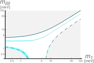
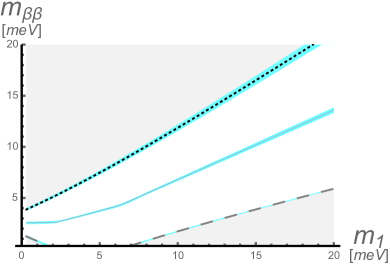
Figure 1: Allowed region for the parameter $m_{\upbeta\!\upbeta}=m_{\rm ee}$ (white) assuming normal mass spectrum. On the left, log-log graph, on right, zoom in the region of the smallest $m_{1}$ somewhat favored by cosmology (see text and Fig. 4 of [122]). The central curve is the average value. The colored bands indicate the uncertainty regions (1 sigma). Gray regions are incompatible with observed neutrino oscillations.

The real trouble is that

the oscillations probe neither the phases of $U_{\ell i}$ nor the mass of the lightest neutrino $m_{1}$.

This implies that the parameter $m_{\rm ee}$ can range from 0 to the maximum value allowed by experimental measurements. The theory of fermion masses (and in particular the one of neutrino masses) is not sufficiently developed to be reliable, and it is difficult to obtain further useful information.

To proceed on an empirical basis, the following steps were taken. In order to address the problem of the phases (sometimes called “Majorana phases”) it was proposed in [121] to consider the maximum and minimum value of $m_{\rm ee}$, by varying the unknown complex phases, obtaining the formulas

$$\begin{array}[]{l}\\[-17.22217pt] \displaystyle m_{\rm ee}^{\mbox{\tiny max}}=\sum_{i=1}^{3}|U_{\rm e\it i}^{2}|\ m_{i}\\[12.91663pt] \displaystyle m_{\rm ee}^{\mbox{\tiny min}}=\mbox{max}\!\left\{\,2\,|U_{\rm e\it i}^{2}|\,m_{i}-m_{\rm ee}^{\mbox{\tiny max}}\,,\,0\,\right\}\end{array}$$ (18)

see Fig. 1 for the standard presentation.

The second problem, namely the fact that the mass of the lightest neutrino is unknown, can be tackled in two ways

• In principle, by means of extremely precise measurements of the absolute neutrino mass $m_{\nu_{\rm e}}^{2}=\sum_{i}|U_{{\rm e}i}^{2}|m_{i}^{2}$ (a parameter discussed in [123, 124, 125, 126, 127]) in the laboratory. Current experiments indicate $m_{\nu_{\rm e}}<0.8-1.1$ eV at 90% and the sensitivity will reach 200 meV in the near future [128]. The current limit directly translate into $m_{1}<0.8-1.1$ eV.

• From cosmology measurements that probe $\Sigma=m_{1}+m_{2}+m_{3}$ as suggested in [129]. Even if they are based on a cosmological model that is conceptually complex and still under verification, the sensitivity of the most recent measurements is just impressive: see e.g. [130, 131, 132]. Proceeding as in [134, 133] we get $\Sigma<100$ [150] meV at 1 [2]$\sigma$ that translates into $m_{1}<20$ [40] meV.

An empirical approach based on cosmological measurement results in a upper bound of $m_{\rm ee}$ of a few 10 meV. This result, obtained and discussed in [134, 133, 122, 135], reinforces the view stated in [39], that it will be a real challenge to be able to observe the electron creation process of Eq. 16. In particular, we can already conclude on this basis that detectors with a mass of many tonnes, and able to operate under stable conditions for many years, will be needed in order to have a chance of detecting the transition due to the Majorana mass of ordinary neutrinos, as argued in [39].

6 Summary and discussion

In this paper, we have retraced some important steps in the understanding of what matter is, according to modern particle physics. We have shown how Majorana’s ideas are rooted right at the heart of the discussion about the question whether it is possible to create particles of matter. Trying to summarise, we could say that the search for the value of Majorana’s neutrino mass is gaining momentum.

We reiterate that we have taken care to touch the main historical lines, but it is important to be aware that at any given time there are forward-looking ideas, rearguard discussions, and even missteps. Obviously, it is not easy to correctly identify one’s position in the present, i.e. at the moment when history is being made, but we believe that having a correct perception of the road already travelled can help to keep the bar in the right direction. In this spirit, and by way of summary, we provide in Tab. 3 a schematic description of the evolution of ideas about what matter is.

We stress that this review has no claim to completeness, and that we have left aside many interesting and widely discussed topics in the scientific literature. Just as a specific example, let us consider the idea that the transition proposed by Furry, Eq. 16, is not due to the Majorana masses of neutrinos, but rather to some other cause. This hypothesis has also been examined and thoroughly discussed: for the first time by Touschek in 1948 [99] (see also [136] and [113]), then just after the discovery of the chiral structure of weak interactions [137], again after the understanding of neutrino oscillations [138], and many other times recently. It is not possible to rebut it on an empirical basis, and current theories are not in a position to exclude it absolutely. Nevertheless, it does not seem possible to argue that it has the same interest as Majorana’s hypothesis, especially in the context of motivated extensions of the standard model, and unless the scale of new physics turns out to be unexpectedly low.

To conclude this discussion, we would like to express an impression somewhat conveyed by this brief historical review: while it is certainly important (essential) to have new experimental facts to discuss, it seems at least as important to have clear and well-defined theoretical ideas to enable real progress, and it is essential to be able to acknowledge and value them. Maybe not a very strong point, but useful to work on.

Finally and quite importantly, it must be said that there is no shortage of tasks for the future, and most of them are quite demanding. In fact, efforts will be needed, devoted 1) to consolidate inferences about the mass of the neutrino (by means of cosmology and laboratory investigations); 2) to continue and to refine the experimental search for the nuclear transition in which two particles of matter (=electrons) are created; 3) to make progress in the evaluation of the nuclear matrix elements related to this transition, quantitatively estimating the errors in expectations; 4) and last but not least, to develop convincing and principled extensions of the standard model, that allow us to obtain useful and reliable indications on the expected value of the Majorana neutrino mass.

matter salient valid reason for components features until inadequacy atoms species, mass [1838] 1909 [atoms of electricity] electron nuclei & e^- charge, mass, spin [1930] 1956 [Fermi th.] neutrons & neutrinos p, n, e, $\nu_{\rm e},$ $\upmu$, … B, L_e, …, " , " [1961] 1968 [standard model] quarks quarks & leptons B-L, L_e-$\mathbf{L}_{\upmu}$, L_μ-$\mathbf{L}_{\tau}$, " , " [1962] 2010 [lepton mixing] appearance exp. quark/antilepton B-L, " , " [1937]      ? [Majorana mass] 2n$\to$2p+2e fermions mass, spin [1977?] ??? [supersymmetry?] ???

Table 3: Table of elementary components of matter according to different models, successive in time. Left columns: brief description. Right ones: shortcomings of the given model. Dates and information [in brackets] refer to mainly theoretical considerations. The current model of what matter is is the one in the penultimate line, since the Majorana mass hypothesis is very reasonable, but does not yet enjoy observational evidence; to date, the limitations of the last model are only speculative.

Appendix A On Majorana spinors

In this appendix, we cover several technical aspects concerning Majorana spinors [4]. Here (as in the rest of this paper) we use consistently Majorana’s representation of the gamma-matrices just as advocated e.g., in [35]. For further discussions see [39, 42]. After introductory matter, Sect. A.1 and A.2, we present in Sect. A.3 the definition of the key parameter, $m_{\rm ee}$. A major obstruction for a useful discussion of Majorana’s neutrino mass, which persisted for more than twenty years, is examined critically in Sect. A.4.

A.1 Illustration of the usefulness of Majorana representation

Thanks to the characteristic feature of Majorana representation of gamma-matrices, all relevant $4\times 4$ matrices have simple properties under conjugation and transposition, given in Tab. 4. This is rather useful in various manipulations.

First example:

Let us begin showing the consistency of Majorana’s condition for a spinor,

$$\bm{\chi}=\bm{\chi}^{*}$$ (19)

The generic Lorentz transformation is parameterized by three angles $\theta_{i}$ and three rapidities $\eta_{i}$:

$$\begin{array}[]{c}\delta\bm{\chi}=\frac{i}{2}\left(\vec{\Sigma}\,\vec{\theta}+\vec{K}\,\vec{\eta}\right)\bm{\chi}\\ \delta\bm{\chi}^{*}=\frac{i}{2}\left(-\vec{\Sigma}^{*}\,\vec{\theta}-\vec{K}^{*}\,\vec{\eta}\right)\bm{\chi}^{*}\end{array}$$ (20)

Since the spin and the boost matrices are both imaginary, as shown in Tab 4, it is evident that $\bm{\chi}$ and $\bm{\chi}^{*}$ transform in the same way.

$\mbox{\textgamma}^{0}$ $\vec{\mbox{\textgamma}}$ $\mbox{\textgamma}^{5}$ $\beta$ $\vec{\alpha}$ $\vec{\Sigma}$ $\vec{K}$ hermiticity + $-$ + + + + $-$ reality $-$ $-$ $-$ $-$ + $-$ $-$ symmetry $-$ + $-$ $-$ + $-$ +

Table 4: Properties of gamma-matrices in Majorana representation. We define as usual $\mbox{\textgamma}^{0}=\beta$ and $\vec{\mbox{\textgamma}}=\beta\,\vec{\alpha}$ from Dirac’s Hamiltonian; $\mbox{\textgamma}^{5}=i\mbox{\textgamma}^{0}\mbox{\textgamma}^{1}\mbox{\textgamma}^{2}\mbox{\textgamma}^{3}$ as chirality matrix; $\Sigma_{jk}=i\mbox{\textgamma}_{j}\mbox{\textgamma}_{k}$. Generators of Lorentz’s group: $\Sigma_{1}=\Sigma_{23}$, $\Sigma_{2}=\Sigma_{31}$, $\Sigma_{3}=\Sigma_{12}$ (spin) and $\vec{K}=i\mbox{\textgamma}^{0}\vec{\mbox{\textgamma}}=i\vec{\alpha}$ (boost). The indices $i,j,k$ take the values $1,2,3$.

Second example:

As a second example of application, let us consider the familiar Lagrangian density of a Dirac field $\bm{\psi}$ (recall that $\hbar=c=1$)

$$\mathcal{L}=\bar{\bm{\psi}}(i\mbox{\textgamma}^{\upmu}\partial_{\upmu}-m)\bm{\psi}={\bm{\psi}}^{\dagger}(i\partial_{0}-i\vec{\alpha}\,\vec{\nabla}-m\beta)\bm{\psi}$$ (21)

where $\upmu=0,1,2,3$, $\partial_{\upmu}=\partial/\partial x^{\upmu}$ and $(\vec{\nabla})^{i}=\partial^{i}$ with $i=1,2,3$. We would like to rewrite $\mathcal{L}$ with Majorana’s fields, still using Majorana’s representation of gamma-matrices. Thus, let us express the Dirac field as follows,

$$\bm{\psi}_{a}=\frac{\bm{\chi}_{a}+i\,\bm{\lambda}_{a}}{\sqrt{2}}\mbox{ where }\bm{\chi}^{*}=\bm{\chi},\ \bm{\lambda}^{*}=\bm{\lambda}$$ (22)

which resembles closely the separation of a complex number into its real and imaginary parts. Various mixed terms appear, but we note that, owing to anticommutativity of the fermionic fields, they are either zero or ‘surface terms’ that can be omitted in the action $S=\int d^{4}x\,\mathcal{L}$,

$$\begin{array}[]{c}\bm{\chi}^{t}\partial_{0}\bm{\lambda}-\bm{\lambda}^{t}\partial_{0}\bm{\chi}=\partial_{0}(\bm{\chi}^{t}\,\bm{\lambda})\\ \bm{\chi}^{t}\alpha^{i}\partial_{i}\bm{\lambda}-\bm{\lambda}^{t}\alpha^{i}\partial_{i}\bm{\chi}=\partial_{i}(\bm{\chi}^{t}\alpha^{i}\bm{\lambda})\\ \bm{\chi}^{t}\beta\bm{\lambda}-\bm{\lambda}^{t}\beta\bm{\chi}=\bm{\chi}^{t}\beta\bm{\lambda}-\bm{\chi}^{t}\beta\bm{\lambda}=0\\ \end{array}$$ (23)

Therefore, the result is equivalent to two decoupled lagrangian densities,

$$\mathcal{L}=\frac{1}{2}\bar{\bm{\chi}}(i\mbox{\textgamma}^{\upmu}\partial_{\upmu}-m)\bm{\chi}+\frac{1}{2}\bar{\bm{\lambda}}(i\mbox{\textgamma}^{\upmu}\partial_{\upmu}-m)\bm{\lambda}$$ (24)

Third example:

From the last formula, we read the Majorana mass term

$$-\frac{m}{2}\bar{\bm{\chi}}\,\bm{\chi}=-\frac{m}{2}\bm{\chi}^{t}\,\mbox{\textgamma}^{0}\,\bm{\chi}$$ (25)

a simple expression that applies for Majorana’s form of gamma matrices. Now we verify explicitly that this term is non-zero, using the components. Let us consider a term in a Lagrangian density with two spinors

$$\bm{\chi}_{a}\,\mbox{\textgamma}^{0}_{ab}\,\bm{\lambda}_{b}=-\bm{\lambda}_{b}\,\mbox{\textgamma}^{0}_{ab}\,\bm{\chi}_{a}=\bm{\lambda}_{b}\,(-\mbox{\textgamma}^{0})^{t}_{ba}\,\bm{\chi}_{a}=\bm{\lambda}_{b}\,\mbox{\textgamma}^{0}_{ba}\,\bm{\chi}_{a}$$ (26)

where in the first step we have used anticommutativity of the spinors, which are quantized fermionic fields, and in the last passage we use antisymmetry of $\mbox{\textgamma}^{0}$, pointed out in the Tab. 4. This calculation might seem pedantic, however is not entirely useless. E.g., consider one statement of [142]: “the scalar $\bar{\psi}\psi$ of the Majorana theory vanishes identically”; when we replace $\bm{\chi}=\bm{\lambda}=\psi$ in Eq. 26, we see that this statement has no valid basis and we can rebut it.
Finally, treating the fields as matrices and applying the usual rules for hermitian conjugation, namely $(\bm{a}\bm{b})^{*}=\bm{b}^{*}\bm{a}^{*}$, we can show that the same term is hermitian (real),

$$(\bm{\chi}_{a}\,\mbox{\textgamma}^{0}_{ab}\,\bm{\lambda}_{b})^{*}=\bm{\lambda}_{b}^{*}\,(\mbox{\textgamma}^{0}_{ab})^{*}\,\bm{\chi}_{a}^{*}=\bm{\lambda}_{b}\,(\mbox{\textgamma}^{0}_{ab})^{*}\,\bm{\chi}_{a}=-\bm{\lambda}_{b}\,\mbox{\textgamma}^{0}_{ab}\,\bm{\chi}_{a}$$ (27)

In the second passage we used the reality condition of Majorana spinors, in the third the fact that $\mbox{\textgamma}^{0}$ is imaginary. Then, applying the same manipulations as in Eq. 26, we conclude the proof of hermiticity – which implies the unitarity of time evolutor.

Fourth example:

Let us consider the coupling of a fermion of Majorana with an external electromagnetic field. In the case of an electrostatic interaction, the hamiltonian density that describes the interaction is

$$\mathcal{H}=q\,A^{\upmu}_{\mbox{\tiny ext}}\bar{\bm{\psi}}\,\mbox{\textgamma}_{\upmu}\bm{\psi}=q\,\varphi\,\bm{\rho}_{\mbox{\tiny ext}}\mbox{ where }\bm{\rho}_{\mbox{\tiny ext}}=\bm{\psi}^{\dagger}\bm{\psi}$$ (28)

Owing to Majorana’s condition, Eq. 19, $\bm{\psi}^{\dagger}\bm{\psi}=\bm{\psi}^{t}\bm{\psi}=\bm{\psi}_{a}\bm{\psi}_{a}=0$ due to anticommutativity. Next let us consider the case of magnetic coupling, namely the hamiltonian density

$$\mathcal{H}=\frac{m}{4}\,F^{\upmu\upnu}_{\mbox{\tiny ext}}\bar{\bm{\psi}}\,\Sigma_{\upmu\upnu}\bm{\psi}=-m\,\vec{B}_{\mbox{\tiny ext}}\,\vec{\bm{S}}\mbox{ where }\vec{\bm{S}}=\frac{1}{2}\bm{\psi}^{\dagger}\mbox{\textgamma}^{0}\,\vec{\Sigma}\bm{\psi}$$ (29)

Now, using Tab. 4, it is easy to prove that the following combination of matrices is symmetric $(\mbox{\textgamma}^{0}\,\vec{\Sigma})^{t}=\vec{\Sigma}^{t}\,(\mbox{\textgamma}^{0})^{t}=\vec{\Sigma}\,\mbox{\textgamma}^{0}=\mbox{\textgamma}^{0}\,\vec{\Sigma}$; thus, the spin operator $\vec{\bm{S}}$ is zero for a Majorana field, again due to anticommutativity of the fermionic fields.

A.2 Dirac and Majorana mass in one-neutrino transitions

We discussed that weak charged interactions, due to their chiral ($V-A$) character, distinguish neutrinos and antineutrinos in the limit where their masses are zero, as in the standard model, and also in the case in the ultrarelativistic limit, if their masses are not zero as is the case. This circumstance in practice limits the possibilities of distinguishing Dirac’s neutrinos from Majorana’s, as we discuss below.

Let us begin by considering the formalism of quantum fields in the case of a Dirac neutrino

$${\bm{\nu}}_{\mbox{\tiny Dirac}}(t,\vec{x})=\sum_{\vec{p}\lambda}\left[{\bm{a}}_{\vec{p}\lambda}\ \psi_{\vec{p}\lambda}\!(t,\vec{x})+{\bm{b}}_{\vec{p}\lambda}^{\dagger}\ \psi_{\vec{p}\lambda}^{*}\!(t,\vec{x})\right]$$ (30)

where $\lambda=\pm 1$ is the helicity of the states, $\psi$ are bispinors of plane waves with positive energies: $\psi_{\vec{p}\lambda}\!(t,\vec{x})=u_{\vec{p}\lambda}\,e^{-i(Et-\vec{p}\,\vec{x})/\hbar}$, the first term describing the creation of a neutrino in the final state and the second term describing the disappearance of an antineutrino in the initial state. We have used Majorana’s representation of matrices, and thus the chirality matrix $\mbox{\textgamma}^{5}=i\mbox{\textgamma}^{0}\mbox{\textgamma}^{1}\mbox{\textgamma}^{2}\mbox{\textgamma}^{3}$ is also imaginary. When we consider a weakly charged interaction, the quantized field is multiplied by the projector $P_{L}=(1-\mbox{\textgamma}^{5})/2$. As well-known (see e.g., [39, 42]) for ultrarelativistic neutrinos the chiral projector selects only bispinors with negative helicity, $P_{L}\,\psi_{\vec{p}\lambda}\approx\psi_{\vec{p}\lambda}$ if $\lambda=-1$ and $P_{L}\,\psi_{\vec{p}\lambda}\approx 0$ if $\lambda=+1$. In correspondence we will have the matrix elements

$$\langle\nu_{\vec{p}\lambda}|P_{L}\,{\bm{\nu}}_{\mbox{\tiny Dirac}}(t,\vec{x})|0\rangle\approx\left\{\begin{array}[]{lc}\psi_{\vec{p}\lambda}&\mbox{ if }\lambda=-1\\ 0&\mbox{ if }\lambda=+1\end{array}\right.\mbox{ when }|\vec{p}|\gg mc$$ (31)

For antineutrino states we will have $P_{L}\,\psi_{\vec{p}\lambda}^{*}=(P_{R}\,\psi_{\vec{p}\lambda})^{*}$ and so antineutrino states with positive (opposite to neutrino) helicity are selected. Neutrinos with positive helicity and antineutrinos with negative helicity do not interact at all - they are sterile.

For Majorana fields, the only change is to identify the operators as follows:

$${\bm{\nu}}_{\mbox{\tiny Majorana}}(t,\vec{x})=\sum_{\vec{p}\lambda}\left[{\bm{c}}_{\vec{p}\lambda}\ \psi_{\vec{p}\lambda}\!(t,\vec{x})+{\bm{c}}_{\vec{p}\lambda}^{\dagger}\ \psi_{\vec{p}\lambda}^{*}\!(t,\vec{x})\right]$$ (32)

The argument exposed in Eq. 31 for Dirac field continues to apply, with two crucial differences

• at the order $m/p$, we can have admixtures with ‘wrong type’ particles (antineutrinos rather than neutrinos or vice versa);

• the operators corresponding to the ‘sterile’ states are completely absent.

Therefore, due to the structure of the weak charged interactions, in the usual case of ultra-relativistic neutrinos (when the mass of neutrinos is small compared to their momentum) the differences between the two types of quantized fields disappear.

A.3 Electron creation and the parameter $m_{\rm ee}$

Consider the semi-leptonic Hamiltonian density leading to the emission of an electron $\mathcal{H}=\sqrt{2}G_{\mbox{\tiny F}}\,\bm{J}^{\mbox{\tiny+}}_{\upmu}\,\bm{j}^{\mbox{\tiny-}\upmu}$, where the leptonic current is

$$\bm{j}^{\mbox{\tiny-}}_{\upmu}=\bar{\bm{e}}\,\mbox{\textgamma}_{\upmu}\bm{\nu}_{\mbox{\tiny Le}}=\sum_{j=1}^{3}U_{\rm e\,\it j}\ \bar{\bm{e}}\,\mbox{\textgamma}_{\upmu}P_{\mbox{\tiny L}}\bm{\chi}_{j}\mbox{ with }\bm{\chi}_{j}=\bm{\chi}^{*}_{j}$$ (33)

where we have postulated that the neutrino mass eingestates are Majorana fields. The leptonic part of the amplitude, that describes the creation of a couple of electrons, is $\langle{\rm e\,e}|{\it T}[\bm{j}^{\mbox{\tiny-}}_{\nu}(x)\bm{j}^{\mbox{\tiny-}}_{\upmu}(y)]|0\rangle$ and it requires to evaluate the contraction $\langle 0|{\it T}[\bm{\nu}_{\mbox{\tiny Le}}(x)\,\bm{\nu}_{\mbox{\tiny Le}}^{t}(y)]|0\rangle$, namely, an unusual type of propagator, that however is non-zero in Majorana’s theory. In fact, from $\bm{\nu}_{\mbox{\tiny Le}}=U_{\rm e\,\it j}\,P_{\mbox{\tiny L}}\bm{\chi}_{j}$, used above, and its transpose, written as $\bm{\nu}_{\mbox{\tiny Le}}^{t}=U_{\rm e\,\it j}\,\bar{\bm{\chi}}_{j}P_{\mbox{\tiny L}}\mbox{\textgamma}^{0}$, the core of the problem reduces to the calculation of an ordinary propagator, namely $\langle 0|{\it T}[\bm{\chi}_{j}(x)\,\overline{\bm{\chi}}_{j}(y)]|0\rangle$. The result is

$$\langle 0|{\it T}[\bm{\nu}_{\mbox{\tiny Le}}(x)\,\bm{\nu}_{\mbox{\tiny Le}}^{t}(y)]|0\rangle=P_{\mbox{\tiny L}}\mbox{\textgamma}^{0}\int\frac{d^{4}p}{(2\pi)^{4}}\frac{i\,U_{\rm e\,\it j}^{2}\,m_{j}\ e^{-ip(x-y)}}{p^{2}-m_{j}^{2}+i\,0^{+}}$$ (34)

The virtual momentum in the denominator has a small time component due to kinematical constraints, whereas the spatial component is of the order of the radius $|\vec{p}|\sim 1/R_{0}$; therefore, the masses of the light neutrinos $m_{j}\ll 100$ MeV are absolutely negligible in the denominator, and the lifetime will depend upon neutrino masses and mixing only through

$$m_{\rm ee}=\left|\sum_{j=1}^{3}U_{\rm e\,\it j}^{2}\,m_{j}\right|=m_{\upbeta\!\upbeta}$$ (35)

we use the same symbols as the ee-element of the neutrino mass matrix, since the two quantities coincide with the phase choice that makes the ee-element real and non-negative. The same quantity is sometimes called ‘effective neutrino mass’ or also ‘electron neutrino mass’, most often indicated with the symbol $m_{\upbeta\!\upbeta}$, which recalls the term ‘(neutrinoless) double beta decay’ but which does not emphasize the connection with neutrino masses. In this way we have covered the key topic, which started ideally with [27] in modern times (after $V-A$) and which was fully completed in [34], with the introduction of $m_{\rm ee}$.

To summarise, it is only possible to distinguish between Dirac and Majorana neutrinos if certain mass-specific effects can be observed, i.e., we depend on a parameter whose value is indisputably small.

A.4 A premature dismissal of Majorana’s ideas

This appendix reconstructs the story of a misunderstanding that began in 1957, the effects of which marred the discussion of Majorana’s neutrinos for a long time. Let us begin by resuming the present situation. Today we are convinced that charged weak interactions have a chiral nature, and guided by the principles of the standard model of elementary particles, we think that the only neutrinos needed to discuss these interactions are the left-handed ones. These positions have no implications for the magnitude of the neutrino’s Majorana mass, which can be constructed from left-handed neutrinos, and which we intend to explore experimentally. To be sure, Eq. 12 consistently describes a non-zero Majorana mass in the context of the (extended) standard model.

In 1957 the discussion was at a much earlier stage, and the problem physicists faced was completely different; they had very little idea what the structure of weak interactions was, and they needed to proceed. In order to do so, they decided to try and explore two hypotheses, i.e., 1) the conservation of the leptonic number and also 2) the absence of mass of the neutrino, which were consistent with the experimental facts known at the time. In this way, a strong and useful theoretical simplification of the structure of neutrino interactions was achieved, which moreover implied that the newly discovered parity violation would apply to neutrinos [143, 144, 145]. These results clarified an important limiting case, but of course, they did not help to quantify in any way what the size of the neutrino mass is. This point is made very clear in [146], a paper of the same year.

Unfortunately, the three seminal articles on the chiral structure of neutrino interactions (appeared just previosly) included very strong statements, which left a lasting impression, that masslessness was an inevitable result and not a hypothesis. E.g., in [21] we read: “Parity violation take places for weak-decays in a specified manner which makes the neutrino self-mass (like the photon self-mass) vanish” and in [23] we read: “A Majorana theory for such a neutrino is therefore impossible. The mass of the neutrino and the antineutrino in this theory is necessarily zero”. Even in [22] (that states in the abstract that masslessness is a hypothesis) we read: “The mass of the longitudinal neutrino, on the other hand, vanishes automatically” which is formally correct, as ‘longitudinal neutrino’ means just a neutrino with fixed helicity in modern parlance, but presents what is a definition as a fact.

Moreover, we must remember the statement against Majorana’s mass made in [142] (which, as discussed in Eq. 26, we now consider to be simply wrong) which casts a doubt on the most conventional formalism, that of bispinors.

As a subsequent examples of prejudices against Majorana, we quote from the abstract of an authoritative work of 1959 [147]: “a verdict may be tentatively reached in favour of a ‘Dirac’ neutrino, operationally distinguishable from a ‘Dirac’ anti-neutrino, and with conservation of total lepton charge valid in all neutrino interactions” and the words of a beautiful paper appeared in 1963 [148] “Konopinsky 1949 estimated the transition probabilities for the cases A and B. He concluded that the probability in case B is about thousand times larger than that of case A. […] This contradicts the experimental data of double beta decay, which favor the Dirac theory”.

The problem got solved only slowly, we refer to the papers already cited and that appeared in a variety of contexts [27, 28, 29, 30, 32, 33, 34, 35, 36, 37, 38]. However, quite surprisingly, the solution was not appreciated universally and some amount of prejudice continued to linger even in recent times. For example, a justly famous book on nuclear physics [149] appeared in 1998 writes about this: “one of the interests in double $\beta$-decay […] is to find out whether neutrinos can be Majorana particles. So far all the evidence seems to suggest that they are strictly Dirac particles”, a statement we do not subscribe for the reasons explained above.

Interestingly, Majorana’s mass always continued to be discussed in the literature but mostly without bispinors, namely adopting the Weyl’s two-dimensional spinor formalism as first done in [150] (who apparently was not aware of Majorana) and above all Case’s work [27] (who instead recognizes Majorana). Case’s paper, which again appeared in 1957, had many merits, among which that of ensuring the consideration/survival of Majorana’s ideas in the scientific literature also in the new context: this is why we mention it in Tab. 2. For instance, this work is cited in the classic book [151], and also in the first calculation of nuclear matrix elements for electron creation/double-beta transition of Eq. 16 in the context of modern $V-A$ theory [28]. Unfortunately, the use of a formalism unfamiliar to a large part of the scientific community in [27] created the impression that, in order to obtain a coherent field theory, it was necessary to reformulate Majorana’s theory with Weyl spinors. However, this is not the case at all: normal bispinors (those with 4 components) are perfectly fine for this purpose, as argued in the main text and in this appendix.

A wider and useful discussion of similar issues is given in [113].

Acknowledgments

I am grateful to Clementina Agodi, Giovanni Benato, Corrado Caselunghe, Silvia de Bianchi, Stefano Dell’Oro and Adriano Di Giovanni for useful discussion. Work partially supported by the research grant number 2017W4HA7S “NAT-NET: Neutrino and Astroparticle Theory Network” under the program PRIN 2017 funded by the Italian Ministero dell’Istruzione, dell’Università e della Ricerca (MIUR). Partly based on presentations [139, 140, 141].

References

- [1] Richard P. Feynman, “The reason for anti-particles” in Elementary particles and the laws of physics, The 1986 Dirac Memorial Lectures, Cambridge U. Pr., 1 (1988)
- [2] Ernst C. G. Stueckelberg, “La signification du temps propre en mécanique ondulatoire” and “Remarque à propos de la création de paires de particules en théorie de relativité” (in French), Helv. Phys. Acta 14 322 and 588 (1941)
- [3] John D. Jackson, Lev B. Okun, “Historical roots of gauge invariance” Rev. Mod. Phys. 73 (2001) 663 (2001)
- [4] Ettore Majorana, “Teoria simmetrica dell’elettrone e del positrone” (in Italian), Nuovo Cim. 14 171 (1937)
- [5] Paul A. M. Dirac, “The quantum theory of the electron” Proc. of R. Soc. London A117 610 (1928)
- [6] Paul A. M. Dirac, “The quantum theory of the electron. Part II” Proc. of R. Soc. London A118 351 (1928)
- [7] Paul A. M. Dirac, “Quantised singularities in the electromagnetic field” Proc. of R. Soc. London A133 60 (1931)
- [8] Murray Gell-Mann, “A schematic model of baryons and mesons” Phy. Lett. 8 214 (1964)
- [9] George Zweig, “An SU(3) model for strong interaction symmetry and its breaking", CERN-TH-401 & 412 (1964). In Developments in the quark theory of hadrons, Vol. 1. 1964 - 1978, Don Bernett Lichtenberg, Simon P. Rosen (ed.) (1980)
- [10] Chen-Ning Yang, “Fermi’s beta-decay theory” Int. J. Mod. Phys. A 27 1230005 (2012)
- [11] Eugene P. Wigner, “Invariance in physical theory” Proc. Am. Philos. Soc. 93 521 (1949)
- [12] George Marx, “Die wechselwirkung der elementar-teilchen und die erhaltungssätze” (in German), Acta Phys. Hungar. 3 55 (1953)
- [13] Yakov B. Zel’dovich, “On the theory of elementary particles. Conservation of the nuclear charge and a possible new type of V-particles” Dokl. Akad. Nauk SSSR 86, 505 (1952). Reprint in Selected works of Ya. B. Zel’dovich, Vol. II: Particles, nuclei, and the Universe, Princeton U. Pr. (1993)
- [14] Emil J. Konopinski, Hormoz M. Mahmoud, “The universal Fermi interaction” Phys. Rev. 92 1045 (1953)
- [15] Tsung-Dao Lee, “History of the weak interactions” CERN Courier, January / February, 7 (1987)
- [16] Ernst C. G. Stueckelberg, “Über die methode der physikalischen naturberschreibung” (in German), Naturforschende Gesellschaf in Basel, Verhandlungen 47 181 (1936)
- [17] Hermann Weyl, “Elektron und gravitation. I” (in German), Zeitschrift für Physik, 56 330 (1929)
- [18] Giulio Racah, “Sulla simmetria tra particelle e antiparticelle” (in Italian), Nuovo Cim. 14 322 (1937)
- [19] Tsung-Dao Lee, Chen-Ning Yang, “Question of parity conservation in weak interactions” Phys. Rev. 104 254 (1956)
- [20] Chien-Shiung Wu, Ernest Ambler, Raymond W. Hayward, Dale D. Hoppes, Ralph P. Hudson, “Experimental test of parity conservation in decay” Phys. Rev. 105 1413 (1957)
- [21] Abdus Salam, “On parity conservation and neutrino mass” Nuovo Cim. 5 299 (1957)
- [22] Lev D. Landau, “On the conservation laws for weak interactions” Nucl. Phys. 3 127 (1957)
- [23] Tsung-Dao Lee, Chen-Ning Yang, “Parity nonconservation and a two component yheory of the neutrino” Phys. Rev. 105 1671 (1957)
- [24] Maurice Goldhaber, Lee Grodzins, Andrew W. Sunyar, “Helicity of neutrinos”, Phys. Rev. 109, 1015 (1958)
- [25] Ennackal Chandy George Sudarshan, Robert E. Marshak, “The nature of the four-fermion interaction” (1957); “Chirality invariance and the universal Fermi interaction” Phys. Rev. 109 1860 (1958), see https://web2.ph.utexas.edu/~gsudama/publications.htm
- [26] Richard P. Feynman, Murray Gell-Mann, “Theory of Fermi interaction” Phys. Rev. 109 193 (1958)
- [27] Kenneth M. Case, “Reformulation of the Majorana theory of the neutrino” Phys. Rev. 107 307 (1957)
- [28] Eugene Greuling, Robert C. Whitten, “Lepton conservation and double-beta decay”, Annals of Physics 11 510 (1960)
- [29] Mikhail G. Shchepkin, “On leptonic charge conservation” (in Russian), Yad. Fiz. 17 820 (1973)
- [30] Bruno M. Pontecorvo, “Mesonium and anti-mesonium” Sov. Phys. JETP 6 429 (1957)
- [31] Bruno M. Pontecorvo, “Inverse beta processes and nonconser-vation of lepton charge” Sov. Phys. JETP 7 172 (1958)
- [32] Samoil M. Bilenky, Jiří Hošek, Serguey T. Petcov, “On oscillations of neutrinos with Dirac and Majorana masses” Phys. Lett. B94 495 (1980)
- [33] Riccardo Barbieri, Jonathan R. Ellis, Mary K. Galliard, “Neutrino masses and oscillations in SU(5)” Phys. Lett. B90 249 (1980)
- [34] Masaru Doi, Tsuneyuki Kotani, Hiroyuki Nishiura, Kazuko Okuda, Eiichi Takasugi, “Neutrino masses and the double beta decay” Phys. Lett. B103 219 (1981)
- [35] Ling-Fong Li, Franck Wilczek, “Physical processes involving Majorana neutrinos” Phys. Rev. D25 143 (1982)
- [36] Joseph Schechter, José W. F. Valle, “Neutrinoless double beta decay in SU(2)U(1) theories” Phys. Rev. D25 2951 (1982)
- [37] Boris Kayser, Robert E. Shrock, Phys. Lett. B112 (1982) 137; “Distinguishing between Dirac and Majorana neutrinos in neutral current reactions” Phys. Lett. B112 137 (1982)
- [38] Boris Kayser, “Majorana neutrinos and their electromagnetic properties” Phys. Rev. D26 1662 (1982)
- [39] Stefano Dell’Oro, Simone Marcocci, Matteo Viel, Francesco Vissani, “Neutrinoless double beta decay: 2015 review” Adv. High Energy Phys. 2016 2162659 (2016)
- [40] Bruno M. Pontecorvo, “Pages in the development of neutrino physics” Sov. Phys. Usp. 26 1087 (1983)
- [41] Samoil M. Bilenky, Tania D. Blokhintseva, Luisa Cifarelli, Victor A. Matveev, Irina G. Pokrovskaya, Mikhail G. Sapozhnikov (ed.) Bruno Pontecorvo selected scientific works (second edition) SIF, Bologna (2013)
- [42] Guido Fantini, Andrea Gallo Rosso, Francesco Vissani, Vanessa Zema, “Introduction to the formalism of neutrino oscillations” Adv. Ser. Direct. High Energy Phys. 28 37 (2018) version updated online in arXiv:1802.05781
- [43] Ko Abe et al. [T2K], “Observation of electron neutrino appearance in a muon neutrino beam” Phys. Rev. Lett. 112 061802 (2014)
- [44] Philip Adamson et al. [NOA], “First measurement of electron neutrino appearance in NOA” Phys. Rev. Lett. 116 151806 (2016)
- [45] Natalia Yu. Agafonova et al. [OPERA], “Evidence for appearance in the CNGS neutrino beam with the OPERA experiment” Phys. Rev. D89 051102 (2014)
- [46] Ko Abe et al. [Super-Kamiokande], “Evidence for the appearance of atmospheric tau neutrinos in Super-Kamiokande” Phys. Rev. Lett. 110 181802 (2013)
- [47] Mark G. Aartsen et al. [IceCube], “Measurement of atmospheric tau neutrino appearance with IceCube DeepCore” Phys. Rev. D99 032007 (2017)
- [48] Murray Gell-Mann, Adam Pais, “Behavior of neutral particles under charge conjugation”, Phys. Rev. 97 1387 (1955)
- [49] Bruno Pontecorvo, “Neutrino experiments and the problem of conservation of leptonic charge” Sov. Phys. JETP 26 984 (1968)
- [50] Yasuhisa Katayama, Ken-iti Matumoto, Sho Tanaka, Eiji Yamada, “Possible unified models of elementary earticles with two neutrinos” Prog. Theor. Phys. 28 675 (1962)
- [51] Ziro Maki, Masami Nakagawa, Shoichi Sakata, “Remarks on the unified model of elementary particles” Prog. Theor. Phys. 28 870 (1962)
- [52] Masami Nakagawa, H. Okonogi, Shoichi Sakata, Akira Toyoda, “Possible existence of a neutrino with mass and partial conservation of muon charge” Prog. Theor. Phys. 30 727 (1963)
- [53] Lincoln Wolfenstein, “Neutrino oscillations in matter” Phys. Rev. D17 2369 (1978)
- [54] Stanislav P. Mikheyev, Alexei Yu. Smirnov, “Resonance amplification of oscillations in matter and spectroscopy of solar neutrinos” Sov. J. Nucl. Phys. 42 913 (1985)
- [55] Bruce T. Cleveland et al. [Homestake] “Measurement of the solar electron neutrino flux with the Homestake chlorine detector”, Astrophys. J. 496 505 (1998)
- [56] Keiko S. Hirata et al. [Kamiokande-II], “Real time, directional measurement of B-8 solar neutrinos in the Kamiokande-II detector”, Phys. Rev. D 44 2241 (1991) [erratum: Phys. Rev. D 45 2170 (1992)]
- [57] Florian Kaether et al. [GALLEX] “Reanalysis of the GALLEX solar neutrino flux and source experiments”, Phys. Lett. B 685 47 (2010)
- [58] Johnrid N. Abdurashitov et al. [SAGE] “Measurement of the solar neutrino capture rate with gallium metal. III: Results for the 2002–2007 data-taking period”, Phys. Rev. C 80 015807 (2009)
- [59] John N. Bahcall, Neutrino astrophysics, Cambridge University Press (1989)
- [60] Alain Bellerive et al. [SNO] “The Sudbury Neutrino Observatory”, Nucl. Phys. B 908 30 (2016)
- [61] Ko Abe et al. [Super-Kamiokande] “Solar neutrino measurements in Super-Kamiokande-IV”, Phys. Rev. D 94 052010 (2016)
- [62] Matteo Agostini et al. [Borexino], “First simultaneous precision spectroscopy of , 7Be, and solar neutrinos with Borexino phase-II”, Phys. Rev. D 100 082004 (2019)
- [63] Azusa Gando et al. [KamLAND] “Reactor on-off antineutrino measurement with KamLAND”, Phys. Rev. D 88 033001 (2013)
- [64] Keiko S. Hirata et al. [Kamiokande], “Observation of a small atmospheric muon-neutrino / electron-neutrino ratio in Kamiokande”, Phys. Lett. B 280 146 (1992)
- [65] Yoichiro Fukuda et al. [Kamiokande], “Atmospheric muon-neutrino / electron-neutrino ratio in the multiGeV energy range”, Phys. Lett. B 335 237 (1994)
- [66] Yoichiro Fukuda et al. [Super-Kamiokande], “Evidence for oscillation of atmospheric neutrinos”, Phys. Rev. Lett. 81 1562 (1998)
- [67] Michelangelo Ambrosio et al. [MACRO], “Measurement of the atmospheric neutrino induced upgoing muon flux using MACRO”, Phys. Lett. B 434 451 (1998)
- [68] Wade W. M. Allison et al. [Soudan-2], “The atmospheric neutrino flavor ratio from a 3.9 fiducial kiloton year exposure of Soudan-2”, Phys. Lett. B 449 137 (1999)
- [69] Moohyun Ahn et al. [K2K], “Indications of neutrino oscillation in a 250 km long baseline experiment”, Phys. Rev. Lett. 90 041801 (2003)
- [70] David Adey et al. [Daya Bay], “Measurement of electron antineutrino oscillation with 1958 days of operation at Daya Bay”, Phys. Rev. Lett. 121 241805 (2018)
- [71] Gyeonghwan Bak et al. [RENO], “Measurement of reactor antineutrino oscillation amplitude and frequency at RENO”, Phys. Rev. Lett. 121 201801 (2018)
- [72] Hervé de Kerret et al. [Double Chooz], “First Double Chooz measurement via total neutron capture detection”, Nature Phys. 16 558 (2020)
- [73] Francesco Capozzi, Eligio Lisi, Antonio Marrone, Antonio Palazzo, Prog. Part. Nucl. Phys. 102 48 (2018)
- [74] Pablo Fernández de Salas, David, Vanegas Forero, Christoph Andreas Ternes, Mariam Tórtola, José W. F. Valle, Phys. Lett. B782 633 (2018)
- [75] Ivan Esteban, Maria Conceptión González-García, Álvaro Hernández-Cabezudo, Michele Maltoni, Thomas Schwetz, JHEP 01 106 (2019)
- [76] Ivan Esteban, Maria Conceptión González-García, Michele Maltoni, Thomas Schwetz, Albert Zhou, “The fate of hints: updated global analysis of three-flavor neutrino oscillations”, JHEP 09 178 (2020)
- [77] Ko Abe et al. [Hyper-Kamiokande Proto-], “Physics potential of a long-baseline neutrino oscillation experiment using a J-PARC neutrino beam and Hyper-Kamiokande”, PTEP 2015 053C02 (2015)
- [78] Fengpeng An et al. [JUNO], “Neutrino physics with JUNO”, J.Phys.G 43 030401 (2016)
- [79] Babak Abi et al. [DUNE], “Deep underground neutrino experiment (DUNE), far detector technical design report, Vol. II DUNE physics”, arXiv:2002.03005 [hep-ex] (2020)
- [80] Sheldon L. Glashow, “Partial symmetries of weak interactions” Nucl. Phys. 22 579 (1961)
- [81] Steven Weinberg, “A model of leptons” Phys. Rev. Lett. 19 1264 (1967)
- [82] Abdus Salam, “Weak and electromagnetic interactions” Proceedings of the 8 Nobel symposium, 367 (1968)
- [83] William Bardeen, “Anomalous Ward identities in spinor field theories” Phys. Rev. 184 1848 (1969)
- [84] Claude Bouchiat, John Iliopoulos, Philippe Meyer, “An anomaly-free version of Weinberg’s model” Physics Letters B38 519 (1972)
- [85] Gerard ’t Hooft, Martinus J. G. Veltman, “Regularization and renormalization of gauge fields” Nucl. Phys. B 44 189 (1972)
- [86] Gerard ’t Hooft, “Symmetry breaking through Bell-Jackiw anomalies” Phys. Rev. Lett. 37 8 (1976)
- [87] Vadim A. Kuzmin, Valery A. Rubakov, Mikhail E. Shaposhnikov, “On anomalous electroweak baryon-number non-conservation in the early universe” Phys. Lett. B155, 36 (1985)
- [88] Keijo Kajantie, Mikko Laine, Kari Rummukainen, Mikhail E. Shaposhnikov, “Is there a hot electroweak phase transition at larger or equal to ?” Phys. Rev. Lett. 77 2887 (1996)
- [89] Peter Minkowski, “ at a rate of 1 out of muon decays?” Phys.Lett. B67 421 (1977)
- [90] Tsutomu Yanagida, “Horizontal gauge symmetry and masses of neutrinos” Proceedings of Workshop on the Baryon Number of the Universe and Unified Theories, 95 (1979)
- [91] Sheldon L. Glashow, “Overview” Summary talk at Neutrino 1979, page 518 (1979)
- [92] Murray Gell-Mann, Pierre Ramond, Richard Slansky, “Complex spinors and unified theories” Proceeding of Supergravity workshop, 315 (1979)
- [93] Rabindra N. Mohapatra, Goran Senjanovic, “Neutrino mass and spontaneous parity nonconservation” Phys. Rev. Lett. 44 912 (1980)
- [94] Jogesh C. Pati, Abdus Salam, “Unified lepton-hadron symmetry and a gauge theory of the basic interactions” Phys. Rev. D 8 1240 (1973)
- [95] Jogesh C. Pati, Abdus Salam, “Lepton number as the fourth color” Phys. Rev. D 10 275 (1974) [erratum: Phys. Rev. D 11 703 (1975)]
- [96] Masataka Fukugita, Tsutomu Yanagida, “Baryogenesis without grand unification” Phys. Lett. B174 45 (1986)
- [97] Steven Weinberg, “Baryon and lepton nonconserving processes” Phys. Rev. Lett. 43 1566 (1979)
- [98] Frank Wilczek, Anthony Zee, “Operator analysis of nucleon decay’ Phys. Rev. Lett. 43 1571 (1979)
- [99] Bruno Touschek, “Zur theorie des doppelten -zerfalls” (in German), Zeitschrift für Physik 125 108 (1948)
- [100] Mark G. Inghram, John H. Reynolds, “Double beta-decay of Te-130” Phys. Rev. 78 822 (1950)
- [101] Ettore Fiorini, Antonino Pullia, Giancarlo Bertolini, Francesco Cappellani, Giambattista Restelli, “A search for lepton nonconservation in double decay with a germanium detector” Phys. Lett. B25 602 (1967)
- [102] Enrico Bellotti, Oilviero Cremonesi, Ettore Fiorini, Claudio Liguori, Stefano Ragazzi, “Multielement proportional chamber for Xe-136 decay” AIP Conference Proceedings 108 42 (1984)
- [103] Mitsuhiro Miyajima, Shinichi Sasaki, Hiroko Tawara, “Search for double beta decay products of Xe-136 in liquid xenon” IEEE Trans. Nucl. Sci. 41 835 (1994)
- [104] Volodymyr I. Tretyak, Yuri G. Zdesenko, “Tables of double beta decay data: An update” Atom. Data Nucl. Data Tabl. 80 83 (2002)
- [105] Yuri G. Zdesenko, “The future of double beta decay research” Rev. Mod. Phys. 74 663 (2003)
- [106] Joannis D. Vergados, Hiroyasu Ejiri, Fedor Šimkovic, “Neutrinoless double beta decay and neutrino mass” Int. J. Mod. Phys. E 25 1630007 (2016)
- [107] Jonathan Engel, Javier Menéndez, “Status and future of nuclear matrix elements for neutrinoless double-Beta decay: A review” Rept. Prog. Phys. 80 046301 (2017)
- [108] Michelle J. Dolinski, Alan W.P. Poon, Werner Rodejohann, “Neutrinoless double-beta decay: Status and prospects” Ann. Rev. Nucl. Part. Sci. 69 219 (2019)
- [109] Volodymyr I. Tretyak, “False starts in history of searches for decay, or discoverless double beta decay” AIP Conf. Proc. 1417 129 (2011)
- [110] Raymond Davis, Jr. “Attempt to detect the antineutrinos from a nuclear reactor by the ClAr reaction” Phys. Rev. 97 766 (1955)
- [111] Wendell H. Furry, “On transition probabilities in double beta-disintegration” Phys. Rev. 56 1184 (1939)
- [112] Maria Goeppert-Mayer, “Double beta-disintegration” Phys. Rev. 48 512 (1935)
- [113] Silvia De Bianchi, “Rethinking antiparticles. Hermann Weyl’s contribution to neutrino physics” Studies in History and Philosophy of Modern Physics 61 68 (2018)
- [114] Hans V. Klapdor-Kleingrothaus, Sixty years of double beta decay: From nuclear physics to beyond standard model particle physics, World Scientific (2001)
- [115] Gianluigi L. Fogli, Eligio Lisi, Daniele Montanino, “A comprehensive analysis of solar, atmospheric, accelerator and reactor neutrino experiments in a hierarchical three generation scheme” Phys. Rev. D49 3626 (1994)
- [116] Francesco Capozzi, Eleonora Di Valentino, Eligio Lisi, Antonio Marrone, Alessandro Melchiorri, Antonio Palazzo, “Global constraints on absolute neutrino masses and their ordering” Phys. Rev. D95 096014 (2017); addendum, Phys. Rev. D101 116013 (2020)
- [117] Azusa Gando et al. [KamLAND-Zen], “Search for Majorana neutrinos near the inverted mass hierarchy region with KamLAND-Zen” Phys. Rev. Lett. 117 082503 (2016)
- [118] Chris Alduino et al. [CUORE], “First results from CUORE: A search for lepton number violation via decay of 130Te,” Phys. Rev. Lett. 120 132501 (2018)
- [119] Oscar Azzolini et al. [CUPID], “Final result of CUPID-0 phase-I in the search for the 82Se neutrinoless double- decay” Phys. Rev. Lett. 123 032501 (2019)
- [120] Matteo Agostini et al. [GERDA], “Final results of GERDA on the search for neutrinoless double- decay” Phys. Rev. Lett. 125 252502 (2020)
- [121] Francesco Vissani, “Signal of neutrinoless double beta decay, neutrino spectrum and oscillation scenarios” JHEP 06 022 (1999)
- [122] Stefano Dell’Oro, Simone Marcocci, Matteo Viel, Francesco Vissani, “The contribution of light Majorana neutrinos to neutrinoless double decay and cosmology” JCAP 12 023 (2015)
- [123] Robert E. Shrock, “New tests for, and bounds on, neutrino masses and lepton mixing” Phys. Lett. B96 159 (1980)
- [124] Bruce H. J. McKellar, “The Influence of mixing of finite mass neutrinos on beta decay spectra” Phys. Lett. B97 93 (1980)
- [125] Igor Y. Kobzarev, Boris V. Martemyanov, Lev B. Okun, Mikhail G. Shchepkin, “The phenomenology of neutrino oscillations” Sov. J. Nucl. Phys. 32 823 (1980)
- [126] Francesco Vissani, “Nonoscillation searches of neutrino mass in the age of oscillations” Nucl. Phys. B Proc. Suppl. 100 273 (2001)
- [127] Yasaman Farzan, Alexei Y. Smirnov, “On the effective mass of the electron neutrino in beta decay” Phys. Lett. B557 224 (2003)
- [128] Max Aker et al. [KATRIN], “Improved upper limit on the neutrino mass from a direct kinematic method by KATRIN” Phys. Rev. Lett. 123 221802 (2019)
- [129] Gianluigi Fogli, Eligio Lisi, Antonio Marrone, Alessandro Melchiorri, Antonio Palazzo, Paolo Serra, Joseph Silk, “Observables sensitive to absolute neutrino masses: Constraints and correlations from world neutrino data” Phys. Rev. D70 113003 (2004)
- [130] Nabila Aghanim et al. [Planck], “Planck 2018 results. VI. Cosmological parameters” Astron. Astrophys. 641 A6 (2020)
- [131] Christophe Yèche et al., “Constraints on neutrino masses from Lyman-alpha forest power spectrum with BOSS and XQ-100” JCAP 06 047 (2017)
- [132] Nathalie Palanque-Delabrouille et al., “Hints, neutrino bounds and WDM constraints from SDSS DR14 Lyman- and Planck full-survey data” JCAP 04 038 (2020)
- [133] Matteo Agostini, Giovanni Benato, Stefano Dell’Oro, Stefano Pirro, Francesco Vissani, “Discovery probabilities of Majorana neutrinos based on cosmological data” Phys. Rev. D103 033008 (2021)
- [134] Stefano Dell’Oro, Simone Marcocci, Francesco Vissani, “Empirical Inference on the Majorana Mass of the Ordinary Neutrinos” Phys. Rev. D100 073003 (2019)
- [135] See the addendum in [116] (2020)
- [136] Jean N.F.J. Serpe, “Sur la théorie abrégée des particules de spin 1/2” (in French) Physica 18 295 (1952)
- [137] Gerald Feinberg, Maurice Goldhaber, “Microscopic tests of symmetry principles” Proc. Natl. Acad. Sci. USA 45 (8) 1301 (1959)
- [138] Bruno Pontecorvo, “Superweak interactions and double beta decay” Phys. Lett. B26 630 (1968)
- [139] Francesco Vissani, “Majorana neutrinos: what, why, where?” invit. sem. at the WIN meeting, Bari, 2019 https://agenda.infn.it/event/13938/contributions/91583/attachments/64054/77749/vissani-win-2019.pdf
- [140] Francesco Vissani, “A history of some recent attempts to go beyond the standard model” invit. sem. at the Workshop Gravity, Information and Fundamental Symmetries of the Max Planck Society, Munich, 2019 https://www.mpi-hd.mpg.de/lin/events/ra-workshop/talks/Vissani-sm.pdf
- [141] Francesco Vissani, “Cos’è la materia per la fisica delle particelle e perché tentare di osservarne la creazione” (in Italian), invit. sem. at the Meeting of the Italian Physics Society (SIF), Milan, 2020 https://www.sif.it/static/SIF/resources/public/files/congr20/ri/Vissani.pdf
- [142] James A. Mc Lennan, Jr., “Parity nonconservation and the theory of the neutrino” Phys. Rev. 106 821 (1957)
- [143] Derek L. Pursey, “Invariance properties of Fermi interactions” Nuovo Cim.6 204 (1957)
- [144] Wolfgang Pauli, “On the conservation of the lepton charge” Nuovo Cim. 6 250 (1957)
- [145] Charles D. Enz, “Fermi interaction with non-conservation of «lepton charge» and of parity” Nuovo Cim. 6 266 (1957)
- [146] Luigi A. Radicati, Bruno Touschek, “On the equivalence theorem for the massless neutrino” Nuovo Cim. 6 1694 (1957)
- [147] Henry Primakoff, Simon P. Rosen, “Double beta decay” Rep. Prog. in Phys. 22 121 (1959)
- [148] Masato Morita, “Theory of beta decay” Prog. Theor. Phys. Suppl. 26 1 (1963)
- [149] Samuel S.M. Wong, Introductory nuclear physics, New York, Wiley (1998)
- [150] Herbert Jehle, “Two-component wave equations” Phys. Rev. 75 1609 (1949)
- [151] Masataka Fukugita, Tsutomu Yanagida, Physics of neutrinos and applications to astrophysics Berlin, Springer (2003)