Intrinsic dimension of path integrals:
data mining quantum criticality and emergent simplicity

Abstract

Quantum many-body systems are characterized by patterns of correlations defining highly non-trivial manifolds when interpreted as data structures. Physical properties of phases and phase transitions are typically retrieved via correlation functions, that are related to observable response functions. Recent experiments have demonstrated capabilities to fully characterize quantum many-body systems via wave-function snapshots, opening new possibilities to analyze quantum phenomena. Here, we introduce a method to data mine the correlation structure of quantum partition functions via their path integral (or equivalently, stochastic series expansion) manifold. We characterize path integral manifolds generated via state-of-the-art Quantum Monte Carlo methods utilizing the intrinsic dimension (ID) and the variance of distances between nearest neighbors configurations (NN): the former is related to data set complexity, while the latter is able to diagnose connectivity features of points in configuration space. We show how these properties feature universal patterns in the vicinity of quantum criticality, that reveal how data structures simplify systematically at quantum phase transitions. This is further reflected by the fact that both ID and variance of NN distances exhibit universal scaling behavior in the vicinity of second-order and Berezinskii-Kosterlitz-Thouless critical points. Finally, we show how non-Abelian symmetries dramatically influence quantum data sets, due to the nature of (non-commuting) conserved charges in the quantum case. Complementary to neural network representations, our approach represents a first elementary step towards a systematic characterization of path integral manifolds before any dimensional reduction is taken, that is informative about universal behavior and complexity, and can find immediate application to both experiments and Monte Carlo simulations.

I Introduction

The path integral (PI) formulation of quantum partition functions is arguably one of the most basic concepts in quantum many-body theory [1, 2, 3]. It provides key and generic information about a given quantum state, typically interpreted via low-order correlation functions. More refined properties, such as the degree of quantum correlations captured by entanglement, can also be extracted from path integrals leveraging on advanced techniques such as the replica trick [4, 5], or by analyzing the topological structure of their degrees of freedom [6]. On a more general, yet abstract ground, the path integral of a many-body problem can be construed as a very complex multi-dimensional manifold embedded in a space that describes both spatial and imaginary-time coordinates: within this geometrical interpretation, while low-order properties of the PI manifold (and their relation to physical observables) are in general well-understood, it is currently unclear if global properties of such data structures can be informative about physical phenomena at all, or if they are constrained by universal properties of the many-body dynamics [3].

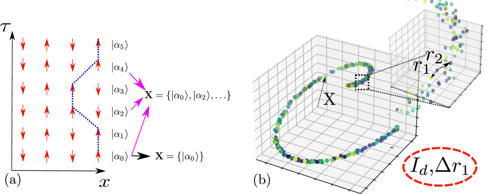
Figure 1: Data structure of quantum partition functions and generic data set features. The partition function of a quantum system can be described by an extended configuration space with one extra dimension $\tau$ (known as imaginary time). As an example, we illustrate in panel (a) a specific space-time configuration of a system with four spins. Each slice $|\alpha_{i}\rangle$ is defined in terms of the spatial degrees of freedom, i.e., $|\alpha_{i}\rangle=(S_{1,i}^{z},...,S_{N_{s},i}^{z})$. Here, we consider data sets generated by either (i) single or (ii) multiple slices. The data structure of quantum partition functions is described by the manifold generated by the set of points ${\bf X}$ in a high-dimensional space. To pictorially explain our approach, we consider in panel (b) a synthetic data set embedded in three dimensions. We investigate generic features of data sets associated to the statistics of nearest- and next-nearest-neighbor configuration distances, $r_{1}$ and $r_{2}$, respectively: namely, the intrinsic dimension, $I_{d}$, and the variance $\Delta r_{1}$ of the distribution function $f(r_{1})$ (see text). Our main result is to show that the $I_{d}$ and $\Delta r_{1}$ exhibit universal critical behavior in the vicinity of different types of quantum phase transitions (see Fig. 2 as an example) and reveal genuine quantum properties (without classical counterpart) of raw data sets.

Here, we show how the full data structure of a path integral (or its related representation as a stochastic series expansion) of certain quantum statistical mechanics models is able to capture genuine quantum effects such as quantum critical behavior [3] as well as properties of quantum phases. We introduce a stochastic characterization of PI manifolds, and study it in the context of quantum spin models by exploiting state-of-the-art techniques from the field of data mining [7], combined with quantum Monte Carlo (QMC) sampling [8, 9]. Our results show how very general properties of the path integral manifold - in particular, its intrinsic dimension [10, 7] - display key signatures of quantum critical behavior in several paradigmatic cases, including second-order and Berezinskii-Kosterlitz-Thouless (BKT) quantum phase transitions. This reveals how universal properties do not only dictate simple path integrals properties such as low-order correlations, but, in fact, govern the entire data manifold - signalling, above all, that quantum phase transitions of spin models are accompanied by structural transitions of the corresponding stochastic description of the path integral. At critical points, the path integral representation is parametrically less complex than those of ordered and disordered phases: quantum criticality is thus accompanied by an emergent simplicity in data space, a fact that offers an alternative angle on the representative power of recently developed neural network states [11, 12, 13].

Before continuing, it is worth stressing that, beyond the basic theoretical goal of characterizing the geometry of path integrals, our approach is directly motivated by recent experimental developments in the field of quantum computing and quantum simulation [14, 15]. While the full characterization of a many-body wave-function via state tomography is experimentally prohibitive (when applicable at all), over the last few years stochastic sampling of wave-functions has become possible in both atomic and solid state platforms [16, 17, 18, 19, 20, 21, 22, 23]. In particular, the combination of high-fidelity in situ imaging techniques and very fast repetition rates has enabled experiments to collect thousands of wave-function snapshots, that, as we argue below, are intimately related to specific types of path integral quantum data sets. These impressive experimental capabilities have already been exploited in a variety of ways, including measurement of entanglement properties and tomography of small partitions [16, 18, 24]. Our approach here differs from these previous attempts, in the fact that we are not targeting specific wave-function properties (such as entropies), but rather, we focus solely on extracting universal information by analyzing the data as a manifold.

The first element in our analysis concerns the definition of proper ’quantum’ data sets describing the path integral manifold. In a previous work [25], some of us have shown how classical partition functions exhibit very specific patterns in data space, that are universal in the vicinity of criticality, and where the corresponding structural transition can be understood utilizing simple arguments based on correlation functions (we note that, while this manuscript was in preparation, two works have appeared [26, 27] that successfully apply the diagnostic we introduced in Ref. [25] to specific forms of wave-function representations). Since PIs can be construed as a highly anisotropic classical partition functions [2], one could naïvely apply methods already developed to understand the latter on the former. However, this turns out to be not only a very inefficient formulation of data mining - as one would have to investigate structural transitions in a data space where one dimension, the imaginary time, is typically very large - but, most relevantly, one that will necessarily mix in an uncontrolled manner real-space and imaginary-time correlations. In addition, the blind application of the ’classical’ procedure will conceal a key aspect of the path integral representation - namely, the fact that quantum mechanical variables do not commute. This last aspect will be particularly important in the presence of non-Abelian symmetries, as we argue below comparing in detail the classical and quantum cases. One thus needs to identify the proper information to be mined, and cannot simply translate from the classical case - irrespectively on how insightful that might be on its own.

We thus introduce two classes of quantum data sets corresponding to the PI stochastic descriptions [see Fig. 1(a)]. The first class is obtained by taking snapshots that are instantaneous in imaginary time, while the second one incorporates within the data set a finite, discrete fraction of imaginary-time "slices". We discuss in detail how both of these choices differ drastically from the equivalent classical description for the two reasons above. Importantly, both data sets are immediately available when sampling partition functions via quantum Monte Carlo methods [28, 29, 2], and the first one is additionally readily obtained from experiments, and from the output of exact and variational wave-function-based methods.

The second part concerns instead the identification and application of the proper tools to characterize the complex data structures correspondent to PIs. The latter are defined in high-dimensional manifolds and may display non-trivial curvature and topology, in addition to inhomogeneous density distributions. The first property of the PI manifold we investigate is the intrinsic dimension - that is, the minimum number of dimensions needed to accurately describe the manifold itself [see Fig. 1(b)]. This allows us to minimally characterize the sampled PI manifold with a single number, that can be efficiently estimated with state-of-the-art algorithms.

For all the models considered here, the intrinsic dimension displays a minimum at transition points - indicating that the geometry of the PI manifold simplifies at criticality. This observation points to the fact that the PI manifold behaves independently from quantum correlations such as bipartite entanglement, that are often maximal at quantum critical points (QCPs) [30, 5]; our findings are instead suggestive of the fact that the PI data structure is inheriting simplicity from the fact that the low-energy properties are captured by very few degrees of freedom (DOF) - and thus, constrain the PI structure. This is reminiscent of the fact that energy spectra are also highly constrained by universal properties: however, while the latter typically depend solely on low-order correlation functions, the constrained structure we observe is related to arbitrary order correlations.

The relation between PI data structure and universal behavior becomes apparent when performing a finite-size scaling (FSS) analysis of the intrinsic dimension [8]: the latter displays universal scaling collapse, whose functional form is dictated by the universality class (second-order or BKT), and by its critical exponent $\nu$. An example of such scaling collapses is illustrated in Fig. 2(a) for the case of BKT transition in the one-dimensional (1D) XXZ spin model, which we investigate below.

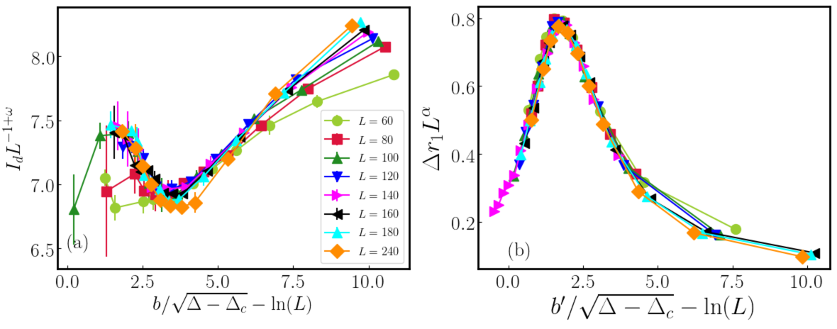
Figure 2: As a representative example of our results, we show the universal data collapse of both the $I_{d}$ [panel (a)] and $\Delta r_{1}$ [panel (b)] for the one-dimensional $1/2$-XXZ model in the vicinity of the Berezinskii-Kosterlitz-Thouless transition (see text).

In addition to the intrinsic dimension, we also investigate the statistical properties of the distances between nearest-neighbor (NN) configurations in the path integral data space. At the qualitative level, the corresponding distribution describes fluctuations of configurations within the path integral manifold: the broader it is, the stronger we expect correlations in our data set - that is, correlations in both space and imaginary time. We show how this quantity - of simpler experimental and computational access than the intrinsic dimension - also provides key signatures of critical behavior [see Fig. 2(b)]. Moreover, beyond the critical regime, we show that it reveals fundamental properties of symmetry-broken phases.

On general grounds, our work aims to learn quantum phases and their transitions in a purely unsupervised manner, i.e., without prior knowledge of the system (e.g., the nature of phases or the phase transitions). While a series of works have recently adopted similar approaches  [31, 32, 33, 34, 35, 36, 37, 38, 15, 39, 40, 41], it is worth mentioning that our route is complementary, and to some extent alternative, to these works, as we access data-based quantities without any projection or compression of the data set. Our approach consists of data mining data sets as a whole, which, as we will illustrate below, allows to access universal properties of quantum systems (while other properties might not be retrievable).

The paper is structured as follows. In Sec. II, we review the formulation of quantum partition functions using path integrals and stochastic series expansions: this allows us to fix notations, and to define the quantum data sets we are interested in. In Sec. III, we introduce the tools we adopt to analyze quantum data sets (i.e., the intrinsic dimension and the statistics of distances) and review the estimators we employ. In Sec. IV and Sec. V, we discuss our analysis of second-order and BKT quantum critical points, respectively. In Sec. VI, we investigate the role of non-Abelian symmetries, and contrast it to the classical case. Finally, in Sec. VII, we draw our conclusions.

II Quantum data sets and models

In order to investigate the properties of our quantum many-body systems of interest, we perform quantum-to-classical mappings which transform the original configurational space of the quantum model into an equivalent classical one, amenable to simulations via appropriate Monte Carlo (MC) algorithms. Subsequently, we analyze the data set of the configurations sampled during the MC simulations via the data-mining-inspired observables mentioned above.

In this section, we offer a discussion of the Hamiltonians studied in our work, with particular focus on their ground-state (quantum) critical behavior, followed by an introduction to the employed quantum-to-classical mappings.

II.1 Models

We analyze the Transverse Field Ising Model (TFIM; see, e.g., [3] for a thorough introduction)

$$H=-2h\sum_{i=1}^{L}S_{i}^{x}-4\sum_{\langle i,j\rangle}S_{i}^{z}S_{j}^{z}$$ (1)

for a one-dimensional system of size $L$ with periodic boundary conditions (PBC), where $S_{i}^{x}$ ($S_{i}^{z}$) denotes the $x$ ($z$) component of the quantum spin-$1/2$ operator $\boldsymbol{S}_{i}$ acting on site $i$, and $\langle i,j\rangle$ denotes a sum over NN pairs of sites. In the ground-state regime, the TFIM undergoes a second-order phase transition at the critical field value $h_{c}=1$ between a paramagnetic and a ferromagnetic (FM) state, corresponding to $h>h_{c}$ and $h<h_{c}$, respectively. Sec. IV A focuses on the determination of the position of the TFIM critical point via data mining of the configurational data set.

We also study the spin-$1/2$ Heisenberg Bilayer model [42, 43], described by the Hamiltonian

$$H=\sum_{a=1,2}\sum_{\langle i,j\rangle}\boldsymbol{S}_{i,a}\cdot\boldsymbol{S}_{j,a}+g\sum_{i=1}^{N_{s}}\boldsymbol{S}_{i,1}\cdot\boldsymbol{S}_{i,2},$$ (2)

where the layer index $a$ identifies one of two symmetrical square lattices of $N_{s}=L\times L$ sites composing the bilayer geometry, and $g$ is the relative strength of the interlayer onsite Heisenberg term with respect to the intralayer NN one. In the ground-state regime, the model displays an $SU(2)$-symmetry-broken antiferromagnetic (AFM) phase and an $SU(2)$-disordered phase for weak and strong $g$, respectively. The transition between these states has been shown to belong to the three-dimensional $O(3)$ (Heisenberg) universality class, and to be characterized by a value of the critical parameter $g=g_{c}=2.5220(1)$, and a correlation length critical exponent $\nu=0.7106(9)$ [43]. The determination of these two quantities via unsupervised learning of the QMC configurational data sets is discussed in Sec. IV B.

Finally, we investigate the one-dimensional spin-$1/2$ XXZ Hamiltonian [44, 45]

$$H=\sum_{i=1}^{N_{s}}\left(S_{i}^{x}S_{i+1}^{x}+S_{i}^{y}S_{i+1}^{y}+\Delta S_{i}^{z}S_{i+1}^{z}\right).$$ (3)

In the $\Delta>0$ region, the phase diagram of the model displays a gapless critical phase for $\Delta<1$, separated from a $\mathbb{Z}_{2}$-symmetry-broken antiferromagnetic phase by a BKT critical point at $\Delta=1$ [44]. The features of this kind of phase transition are radically different from those of second-order criticality such as the examples mentioned above, and include, e.g., the non-locality of the order parameter associated to the transition, as well as an exponential (rather than power-law) divergence of the correlation length in proximity of the transition. The results of our application of data-mining-related observables to the study of this kind of critical behavior in the one-dimensional XXZ model are discussed in Sec. V.

II.2 Quantum-to-classical mappings and quantum data sets

The partition function of a quantum system described by a Hamiltonian $H$ is

$$Z=\sum_{\left\{|\alpha\rangle\right\}}\langle\alpha|e^{-\beta H}|\alpha\rangle,$$ (4)

where $\beta=1/T$ is the inverse temperature of the system (in units of the Boltzmann constant), and $\left\{|\alpha\rangle\right\}$ is a complete basis set for the Hilbert space in which $H$ operates. In the following, we will employ a basis set in terms of the eigenvalues of $S^{z}$ operators: $|\alpha\rangle=(S_{1}^{z},...,S_{N_{s}}^{z})$ for all models considered. In the MC approaches considered in this work, many-body configurations are sampled with a probability proportional to their contribution to the partition function, making the evaluation of terms such as those in the sum in Eq. (4) crucial.

The first of the MC techniques adopted in this work is known as Path Integral Monte Carlo (see, e.g., [28]), and allows a direct, unbiased sampling of the Path Integral manifold. In this approach, the Hamiltonian of the original quantum system is decomposed as $H\equiv H_{0}+H_{1}$, where the two terms are diagonal and non-diagonal on the basis set formed by the $|\alpha\rangle$, respectively: the partition function in Eq. (4) can then be rewritten as

$$Z=\sum_{\left\{|\alpha\rangle\right\}}\langle\alpha|\prod_{k=0}^{M-1}e^{-\epsilon\left(H_{0}+H_{1}\right)}|\alpha\rangle$$ (5)

$$=\sum_{\left\{|\alpha_{k=1,\ldots,M}\rangle\right\}}\prod_{k=0}^{M-1}\langle\alpha_{k}|e^{-\epsilon H_{0}}e^{-\epsilon H_{1}}|\alpha_{k+1}\rangle+O\left(\epsilon^{2}\right)$$

$$=\sum_{\left\{|\alpha_{k=1,\ldots,M}\rangle\right\}}\prod_{k=0}^{M-1}e^{-\epsilon\langle\alpha_{k}|H_{0}|\alpha_{k}\rangle}\langle\alpha_{k}|e^{-\epsilon H_{1}}|\alpha_{k+1}\rangle+O\left(\epsilon^{2}\right),$$ (6)

where $\epsilon\equiv\beta/M$, each of the sets $\left\{|\alpha_{k}\rangle\right\}$ is a complete set for the Hilbert space, and $|\alpha_{M}\rangle\equiv|\alpha_{0}\rangle$.

For quantum spin systems, such as those considered in our work, the states $|\alpha_{k}\rangle$, also known as slices, are usually chosen as eigenvectors of the $z$-component of the quantum spin-$1/2$ operators $\boldsymbol{S}_{i}$ acting on each site $i$, i.e., $|\alpha_{k}\rangle\equiv|S_{1k}^{z},\ldots,S_{N_{s}k}^{z}\rangle$, where $N_{s}$ is the system size. The union of the various sets $\left\{|\alpha_{k}\rangle\right\}$ in Eq. (6) can be interpreted as an extended configuration space, whose dimensionality is increased by 1 with respect to the one of the original quantum system, and whose MC sampling can be performed via a conventional Metropolis algorithm due to the relative simplicity of the calculation of the matrix elements in Eq. (6). In the following, we adopt the PIMC technique to analyze the one-dimensional TFIM described by the Hamiltonian in Eq. (1), which is mapped by the procedure discussed above to a two-dimensional, classical, anisotropic Ising model. The configuration space of the latter is then sampled via the use of conventional Wolff cluster updates [46].

As discussed in the Introduction, our approach is based on the analysis of generic features of the data structure associated with classical representations of quantum partition functions [the definition of the data structure is shown in Fig. 1(a)]. The PI represents one choice for such representation. However, to demonstrate the flexibility of our procedure, we analyze some of our models of interest using an equivalent and related representation to the PI one: namely, the Stochastic Series Expansion (SSE) approach (see, e.g., [47]).

In this method, the quantum partition function in Eq. (4) is rewritten by expanding the exponential operator in power series of $H$

$$Z=\sum_{k=0}^{\infty}\frac{(-\beta)^{k}}{k!}\sum_{\left\{|\alpha\rangle\right\}}\langle\alpha|H^{k}|\alpha\rangle$$

$$=\sum_{k=0}^{\infty}\frac{(-\beta)^{k}}{k!}\sum_{\left\{|\alpha_{k}\rangle\right\}}\langle\alpha_{0}|H|\alpha_{k-1}\rangle\times\langle\alpha_{k-1}|H|\alpha_{k-2}\rangle\times...$$

$$\times\langle\alpha_{2}|H|\alpha_{1}\rangle\times\langle\alpha_{1}|H|\alpha_{0}\rangle,$$ (7)

where the definition and constraints on the $\left\{|\alpha_{k}\rangle\right\}$ are the same as in Eq. (6). As in the PI case, the ensemble of the $\left\{|\alpha_{k}\rangle\right\}$ can be interpreted as a higher-dimensional configuration space; a schematic representation of the latter as obtained by applying the SSE (or PI) mapping is displayed in Fig. 1(a).

As all the matrix elements in Eq. (7) are easily evaluated (and positive-definite in the case of the models considered here), the configuration space is now amenable to importance MC sampling according to the partition function, which in the following is performed via a combination of diagonal and off-diagonal directed-loop updates [48].

The two mappings described above can be proven to be identical in the limit $M\to\infty$ [49]. On the one hand, if one takes the SSE partition function in Eq. (7), chooses a “cut-off” $k_{\max}=M$ for the expansion order, and adds $(M-k)$ matrix elements of the identity to each term of order $k$, one obtains

$$Z_{\mathrm{SSE}}=\sum_{\left\{S_{M}\right\}}\sum_{\left\{|\alpha_{k}\rangle\right\}}\frac{\beta^{k}(M-k)!}{M!}\langle\alpha_{0}|H_{i_{M}}|\alpha_{M-1}\rangle\times\ldots$$

$$\times\langle\alpha_{2}|H_{i_{2}}|\alpha_{1}\rangle\langle\alpha_{1}|H_{i_{1}}|\alpha_{1}\rangle,$$ (8)

where $\left\{S_{M}\right\}$ identifies the ensemble of all sequences of length $M$ of operators $H_{i}$, the indices $i=0,1$ denotes the identity or the Hamiltonian operator, respectively, and the combinatorial factor $M!/\left[k!(M-k)!\right]$ has been introduced to keep into account the equivalent ways to insert the $(M-k)$ identity operators in the $M$-sized operator string.

On the other hand, the partition function in Eq. (4) can be rewritten, starting from Eq. (5), as

$$Z_{\mathrm{PI}}=\sum_{\left\{|\alpha_{k}\rangle\right\}}\langle\alpha_{0}|1-\epsilon H|\alpha_{M-1}\rangle\times\ldots$$

$$\times\ldots\times\langle\alpha_{2}|1-\epsilon H|\alpha_{1}\rangle\langle\alpha_{1}|1-\epsilon H|\alpha_{0}\rangle+O\left(\epsilon\right)$$ (9)

The terms can then be rearranged, using the notations introduced in Eq. (8), as

$$Z_{\mathrm{PI}}=\sum_{\left\{S_{M}\right\}}\sum_{\left\{|\alpha_{k}\rangle\right\}}\epsilon^{k}\langle\alpha_{0}|H_{i_{M}}|\alpha_{M-1}\rangle\times\ldots$$

$$\times\ldots\times\langle\alpha_{2}|H_{i_{2}}|\alpha_{1}\rangle\langle\alpha_{1}|H_{i_{1}}|\alpha_{0}\rangle+O\left(\epsilon\right)$$ (10)

In the limit $M\to\infty$, the prefactor $\beta^{k}(M-k)!/M!$ in (8) converges to $\beta^{k}/M^{k}=\epsilon^{k}$, while the approximation error in (10) vanishes, implying the equivalence of the expressions for $Z$ obtained in the two formalisms. In our calculations, with both the PI and SSE approach, we increase the number of slices until finite-$M$ effects are negligible, ensuring the attainment of the limit mentioned above, and therefore the equivalence of the PI and SSE methods to analyze our problems of interest in the regimes investigated in this study.

The data sets analyzed in our work are composed by stochastically sampled elements of the extended configuration spaces discussed above, written in terms of the the set of slices $\{|\alpha_{i}\rangle\}$. More specifically, we consider sets of either

• single-slice configurations $\vec{X}=\left\{|\alpha_{0}\rangle\right\}$, or

• configurations containing a subset of $M^{\prime}\leq M$ evenly spaced slices, i.e., $\vec{X}=\left\{|\alpha_{k_{1}}\rangle,...,|\alpha_{k_{M^{\prime}}}\rangle\right\}$, where $k_{i}\equiv i\times\left[M/M^{\prime}\right]$, $i=0,\ldots,M^{\prime}-1$, and $[x]$ denotes the integral part of a real number $x$ (see Fig. 1).

As anticipated in the introduction, the first data set also corresponds to wave-function snapshots in experiments with in situ imaging, while the second data set genuinely displays path integral features, incorporating effects from imaginary-time correlations.

III Data mining quantum data sets

We investigate generic features of data sets aiming to extract useful information about quantum criticality. More specifically, we consider basic data set features associated with the statistics of distances between neighboring configurations: namely, the intrinsic dimension and the variance of the distribution of neighbouring distances. Below, we describe in more detail the key quantities and discuss their connections with physical properties of quantum phase transitions.

III.1 Intrinsic dimension and two-NN estimators

A common way to deal with data sets is to consider each data instance as a point in a space whose dimension (the embedding dimension, $N_{c}$) is the number of features needed to describe each sample. However, the existence of correlations between data points usually leads to situations in which the points live, approximately, in a manifold whose dimension, known as intrinsic dimension (ID) and denoted by $I_{d}$, is much lower than $N_{c}$. The basic intuition behind the $I_{d}$ is illustrated in Fig. 1: although the synthetic data set of panel (b) is embedded in a 3D space, its essential content can be described (almost without loss of information) by a non-linear manifold whose $I_{d}$ is equal to 1. In simple cases like this, the $I_{d}$ corresponds to the minimum number of variables needed to describe a data set.

Different approaches have been proposed to estimate the $I_{d}$; see Ref. [10] for an extensive discussion about this topic. The technique used here, the TWO-NN [7], is based on a class of methods that relies on the statistics of distances between NN elements in the data set. The basic idea of such approaches is that nearest-neighborhood points can be considered as uniformly drawn $I_{d}$-dimensional hyperspheres [10, 50]. This assumption allows one to establish relations between the $I_{d}$ and the statistics of neighboring distances. In particular, in the TWO-NN, for each point $\vec{X}$ in the data set [see Fig. 1 (b)] one considers its distance from its NN and next-nearest-neighbor (NNN) point $r_{1}(\vec{X})$ and $r_{2}(\vec{X})$, respectively. The set of distances $r_{1}$ and $r_{2}$ are defined in terms of the Euclidean distance (see below). Under the condition that the data set is locally uniform in the range of next-nearest-neighbors, it has been shown in Ref. [7] that the formula for the distribution function of ${\mu=r_{2}(\vec{X})/r_{1}(\vec{X})}$ is

$$f(\mu)=I_{d}\mu^{-I_{d}-1}$$ (11)

or, in terms of the cumulative distribution $P(\mu)$,

$$I_{d}=-\frac{\ln\left[1-P(\mu)\right]}{\ln\left(\mu\right)}.$$ (12)

Due to the minimal extension of the neighborhood considered, the TWO-NN method is particularly suitable for non-linear manifolds, which is important when dealing with physical data sets [25].

It is worth mentioning that the TWO-NN is designed for configurations defined on a continuous support. However, the generalization to configurations describing discrete data sets, such as those considered in this work, is straightforward and does not display problems if a large enough number of coordinates $N_{c}$ is considered.

Before proceeding, let us define more precisely the quantum data sets introduced at the end of last section. As described in Fig. 1, such data sets are defined by a set of points $\vec{X}^{i}=(X^{i}_{1},X^{i}_{2},...,X^{i}_{N_{c}})$, where the index $i$ is the label of the configurations sampled in the MC simulations (i.e., $i=1,...,N_{r}$), $N_{c}$ is the number of coordinates (or the embedding dimension, as mentioned above), and $N_{r}$ is the total number of points considered in the data sets. The coordinates $X^{i}_{j}$ are defined in terms of the path integral (or stochastic series expansion) degrees of freedom, as explained in Fig. 1(a) and in Sec. II.2.

III.2 Scale dependence of the $I_{d}$ and the statistics of neighbouring distances

One key aspect is that the $I_{d}$ (computed via the TWO-NN method) is a scale-dependent quantity. More specifically, the $I_{d}$ is measured on a range scale defined by the NN and NNN distances $r_{1}$ and $r_{2}$ [7]. For each point in the phase diagram, the scale is determined by the total number of points in configuration space, $N_{r}$, since the latter fixes the average values of $r_{1}$ and $r_{2}$. Indeed, the effect of changing $N_{r}$ is analogous to zooming in or zooming out the data set in configuration space, which changes the value of $I_{d}$ [see the pictorial example in Fig. 1(b)]. The $I_{d}$ also reveals changes of scale associated with structural transitions in configuration space. For example, we mention the structural transitions occurring in classical data sets in proximity of thermal phase transitions [25].

The fundamental reason why the $I_{d}$ exhibits a singular behavior in the vicinity of classical transitions is related to changes of scale in configuration space [25], which interestingly can be associated to significant changes in the physical properties of the connectivity of neighboring points. For example, in the case of the classical Ising transition the data structure related to Ising ferromagnetic phases is characterized by configurations whose NN and NNN have essentially equivalent physical properties (e.g., magnetization): conversely, in the disordered phase the physical properties of neighboring configurations are entirely uncorrelated. A similar reasoning applies in the case of a the classical BKT transition, where neighboring points are characterized by configurations with the same topological properties (i.e., winding number) in the ordered phase.

The reasoning mentioned above serves as a guideline for defining other quantities associated with the statistics of neighboring distances. As we discuss below, such quantities (going beyond the $I_{d}$) reveal essential properties of path integral data sets. More specifically, we consider the distribution function associated to the NN (NNN) distances, and its variance $\Delta r_{1}$ ($\Delta r_{2}$):

$$\Delta r_{i}=\left<r_{i}^{2}\right>-\left<r_{i}\right>^{2},$$ (13)

where $\left<r_{i}\right>=N_{r}^{-1}\sum_{k=1}^{N_{r}}r_{i}(\vec{X^{k}})$, (with $i=1,2$); $r_{1}(\vec{X^{k}})$ and $r_{2}(\vec{X^{k}})$ are the first and the second nearest-neighbor distances associated to the configuration $\vec{X^{k}}$, respectively. At least in the case where the data sets are homogeneous in density, the $\Delta r_{i}$ can detect changes of scale in configuration space, similarly to the $I_{d}$. Furthermore, the $\Delta r_{i}$ reflects the global connectivity of neighboring points in configuration space, which is a fundamental ingredient to detect topological transitions [33]. We note that the $\Delta r_{i}$, differently from $I_{d}$, are also sensitive to inhomogeneity in the sampling of the data set: therefore, in general we expect $I_{d}$ to provide a more reliable description of universal properties.

III.3 Distances and correlations

A crucial step to obtain both the $I_{d}$ and $\Delta r_{i}$ is to consider a proper metric. Here, we compute the distance $r(\vec{X}^{i},\vec{X}^{j})$ between two configurations $\vec{X}^{i}$ and $\vec{X}^{j}$ according to the well-known Euclidean metric, following which the distance can be straightforwardly recast in the form

$$r(\vec{X}^{i},\vec{X}^{j})=\sqrt{2N_{c}\left(1-\frac{1}{N_{c}}\sum_{p=1}^{N_{c}}X^{i}_{p}X^{j}_{p}\right)}.$$ (14)

This choice satisfies the basic requirements for a proper metric: namely, it is non-negative, equal to zero only for identical configurations, symmetric, and it respects the triangular inequality.

It is worth mentioning that the Hamming distance is also a proper metric, which could be used in place of the Euclidean one leading to only a trivial change in the intrinsic dimension for the data sets considered in our work (i.e., binary variables): more specifically, $I_{d}^{E}=2I_{d}^{H}$, where $I_{d}^{E}$ and $I_{d}^{H}$ are the intrinsic dimension computed with the Euclidean and the Hamming metric, respectively. This result can be understood if we (i) define the Euclidean and Hamming distances between two configurations as $r^{E}=2\sqrt{N_{\mathrm{diff}}}$ and $r^{H}=N_{\mathrm{diff}}$, where $N_{\mathrm{diff}}$ is the number of unequal coordinates of the configurations, and (ii) consider that the ID is a function of $\ln(r_{2}/r_{1})$ (see Eq. (12)).

An advantage of considering a standard metric (such as the Euclidean distance) is that we can efficiently compute the set of NN distances $r_{1}$ and $r_{2}$ with state-of-the-art unsupervised NN search algorithms, leading to $O\left(N\log(N)\right)$ scaling of the computational complexity [51]. However, it is worth mentioning that $r(\vec{X}^{i},\vec{X}^{j})$ does not reflect the underlying symmetries of the physical configurations $\vec{X}$. For instance, here we consider systems with translation symmetry (in space and imaginary-time direction), for which the distance between two configurations $\vec{X^{i}}$ and $\vec{X^{j}}$ related by a given translation symmetry operation should be equal to zero. As a simple example, let us consider $\vec{X^{i}}=(-1,-1,-1,1)$ and $\vec{X^{j}}=(-1,1,-1,-1)$: despite these configurations being physically equivalent by translational symmetry, we have $r(\vec{X}^{i},\vec{X}^{j})>0$. Nevertheless, this drawback does not affect our results, given that the probability of sampling two or more configurations belonging to the same translational symmetry sector is exponentially suppressed for large number of configurational DOF (typically, we consider $N_{c}>100$).

One key aspect of the form of $r(\vec{X}^{i},\vec{X}^{j})$ displayed in Eq. (14) is that it reveals the intimate relation between generic data set features and correlations described by the terms $X^{i}_{p}X^{j}_{p}$. An interesting perspective is to try to connect such data correlations with correlations between the variables themselves, i.e., correlations of the type $X^{i}_{p}X^{i}_{r}$, where $p$ and $r$ are indices related to the coordinates of a given configuration vector $i$. From now on, we call the later physical correlations; for the quantum data sets considered here, the indices $p$ and $r$ may be separated by distances in both space and/or imaginary time. Although it is hard to establish this connection in general, one can verify that it indeed holds in certain temperature regimes of classical systems [25], which explains (at least qualitatively) why the $I_{d}$ and quantities related to the statistics of neighboring distances exhibit universal scaling behavior in the vicinity of classical critical points. However, whether or not such a connection holds for quantum systems, or if generic features of the data sets are related to universal properties of quantum critical points, cannot be immediately answered based on the classical results. As we discuss now, quantum data sets differ in a fundamental way from their classical counterparts.

III.4 Differences between quantum and classical partition-function data sets

The path integral of a $D$-dimensional partition function can be mapped to a (highly-anisotropic) classical partition function in $D+1$ dimensions. It is thus natural to wonder whether one could just employ the same methods already applied to study the latter in the context of the former. The answer is negative for three main reasons - two of conceptual and one of practical nature.

The first limitation is that analyzing PIs as classical data sets will necessarily mix information contained in space and imaginary-time correlations: this will make it hard to identify precise connections between the data structure itself and physical phenomena, as it will correspond to analyzing arbitrary space- and time- correlations. The reason why identifying such connections would be challenging is that physical information (such as critical exponents) is typically referred to specific correlation functions in either in space or in time: for instance, the correlation length critical exponent $\nu$ is associated to equal-time correlators, while certain anomalous critical exponents are related to the decay of single-site Green functions in imaginary time. This is in sharp contrast with the classical case, where correlations are isotropic. Analyzing the full PI manifold would unavoidably mix these two types of relevant information.

The second limitation is that only a given part of the PI manifold is experimentally accessible. This is, to the best of our knowledge, a consequence of the fundamentally quantum nature of the problem: once wave-function snapshots are taken, these are necessarily in the form of strong measurements.

The third limitation is of practical nature. Data mining a manifold becomes impractical when the dimension of the embedding data space increases. A priori, this does not seem an issue, as the number of points necessary to characterize the intrinsic dimension of a manifold is typically related to the dimension of the manifold itself, and not to that of the embedding space. A simple example of this fact is the identification of a line in a $D$-dimensional space, for which one just needs a number of points that scales with the intrinsic dimension. However, in practical terms, one still requires a larger number of samples to properly characterize the manifold features, especially for the very large values of the intrinsic dimensions we will encounter below.

The three considerations above highlight the fact that one cannot simply take the same approach demonstrated with classical partition functions, and apply it to PI manifolds: in the best case, this would lead to a hard-to-decipher and experimentally inaccessible picture, while in the worst-case scenario the classically-mutuated approach will be simply inapplicable. The quantum data sets described above overcome these limitations at different levels, via either focusing on a single slice, or capturing imaginary-time properties in a selective manner.

There is an additional, genuinely quantum-mechanical aspect that quantum data sets have to handle: namely, the fact that quantum fields do not commute. Since the definition of the data set requires specifying a given basis, this will inevitably lead to new features in the presence of non-Abelian symmetries, as the latter are characterized by non-commuting conserved quantities. In Sec. VI, we will address this specific aspect in the context of SU(2) symmetries.

IV Second-order transitions

We begin by considering the behavior of both the $I_{d}$ and the NN distance distribution variance $\Delta r_{1}$ in the vicinity of two paradigmatic examples of second-order quantum phase transitions.

IV.1 One-dimensional quantum Ising model

In this section we discuss the results of the application of the observables introduced in Sec. III to the analysis of the quantum critical behavior of the one-dimensional TFIM (see Sec. IIB). The required configuration data sets are generated via PIMC simulations performed at inverse temperature $\beta=512$, where convergence in temperature to the ground state regime was observed for the order parameter associated to the ferromagnetic transition [i.e., the squared magnetization $m_{z}^{2}=\frac{4}{L^{2}}\left(\sum_{i=1}^{L}S_{i}^{z}\right)^{2}$]. All the simulations considered in the following are performed with $M=131072$ slices, of which $M^{\prime}=512$ are considered in the configurations which compose the analyzed data set.

In order to ensure a thorough enough sampling of the $L\times M^{\prime}$ DOF in each of the configurations, we sample $N_{r}=32768$ configurations for each of our simulations, which is more than or equal to twice the number of DOF in any of the cases we analyze. These configurations are sampled at regular intervals in MC time (i.e., the distance between them in number of updates is constant). To avoid correlated sampling, for each of our simulations we compute the autocorrelation time of one of the DOF (assuming a weak dependence of such a quantity on this choice) and continue the simulation until it is possible to extract $N_{r}$ configurations such that the distance in simulation time between them is larger than or equal to the estimated autocorrelation time.

The first step in our analysis is the direct calculation of the $I_{d}$ of the sampled configurations. The results for different system sizes are shown in Fig. 3(a) as a function of the transverse field $h$. The most striking feature of the behavior of the $I_{d}$ here is the presence of a minimum at a size-dependent value of the field $h^{*}(L)<h_{c}$, which for larger sizes progressively moves towards the critical point. We perform a linear fit of the position of this minimum in the thermodynamic limit $L\to\infty$ [see brown triangles in Fig. 3(c)] obtaining an extrapolated value $h^{\infty}=1.045(7)$.

In order to compare the accuracy of the $I_{d}$ estimate for the transition point with that obtainable via conventional FSS analysis, we compute the variance of the magnetization distribution along the $x$ axis

$$\chi_{x}\equiv L\beta\left(\langle m_{x}^{2}\rangle-\langle\left|m_{x}\right|\rangle^{2}\right),$$ (15)

where $m_{x}\equiv\frac{2}{L}\sum_{i=1}^{L}S_{i}^{x}$. This quantity can be calculated by exploiting the self-duality of the one-dimensional TFIM under an axis rotation mapping the $x$ axis into the $z$ axis. In particular, this property results in the identity between $m_{x}$ computed at a value $h$ of the transverse field and $m_{z}$ computed at $h^{\prime}=1/h$, with the latter being straightforward to obtain in the PIMC approach.

The observable $\chi_{x}$ is reminiscent of the susceptibility for a classical $\mathbb{Z}_{2}$-symmetry-breaking phase transition. Indeed, it also shares a similar finite-size behavior (see, e.g., [48]), peaking at a size-dependent value $h^{*}_{\chi}(L)<h_{c}$ of the transverse field which approaches the exact critical point as the size increases [see Fig. 3(b)], a behavior which, as discussed above, is also displayed by the $I_{d}$. A linear extrapolation of the finite-size peak positions as a function of the inverse size [see green squares in Fig. 3(c)] returns an extrapolated value $h^{\infty}_{\chi}=1.02(1)$. The latter displays comparable accuracy to the $I_{d}$ estimate obtained using the same system sizes, proving the substantial equivalence in precision between FSS of the $I_{d}$ and that of more conventional observables usually associated to critical behavior.

In order to gather more insight about the behavior of the configurations in the proximity of the critical point, we compute the variance $\Delta r_{1}$ of the distribution of the recorded distances between each configuration in the data set and its NN; our results for this quantity for various system sizes are shown in Fig. 4(a) as a function of the transverse field. The variance $\Delta r_{1}$ displays a peak at a size-dependent position $h^{m}(L)$, with the distribution $f(r_{1})$ correspondingly displaying significant broadening when approaching the critical point [Fig. 4(b)]. The $h^{m}(L)$ are not necessarily identical to the $h^{*}(L)$, but display the same behavior, gradually approaching the critical point for increasing system size. Performing a linear fit as in the case of the $I_{d}$ minimum position [see Fig. 4(c)], we obtain the extrapolated value $h^{m}(\infty)=1.03(1)$. The variance of the distribution for the distance of each configuration to its NNN in the sampled data set (not shown) displays an essentially identical behavior, and a fit performed in the same fashion as above yields an extrapolated value $h_{\infty}^{m}=1.04(1)$ for the peak position in the thermodynamic limit.

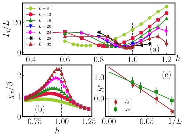
Figure 3: Quantum Ising model (Intrinsic dimension). Panel (a): intrinsic dimension $I_{d}$ in units of the system size $L$ as a function of $h$. Panel (b): magnetization variance in the $x$ direction as a function of the transverse field $h$. Panel (c): extrapolation to the thermodynamic limit of the position of the $I_{d}$ minima $h^{*}(L)$ and of the susceptibility peaks $h_{\chi}^{*}(L)$ as a function of $1/L$; we obtain $h^{\infty}=1.045(7)$ and $h^{\infty}_{\chi}=1.02(1)$, respectively. In all panels, the vertical dashed line corresponds to the critical point $h=h_{c}$.

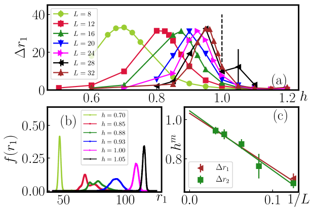
Figure 4: Quantum Ising model (statistics of NN distances). Panel (a): variance $\Delta r_{1}$ of the distribution function of the NN distances $f(r_{1})$ as a function of $h$. Panel (b): $f(r_{1})$ for $L=16$ as a function of $h$. Panel (c): extrapolation to the thermodynamic limit of the position of the maxima $h^{m}(L)$ of $\Delta r_{1}$ (and $\Delta r_{2}$) as a function of $1/L$; ; we obtain $h^{m}_{\infty}=1.03(1)$ [and $h^{m}_{\infty}=1.04(1)$]. In all panels, the vertical dashed line corresponds to the critical point $h=h_{c}$.

Remarkably, we observe that the singular features associated with both the $I_{d}$ and $\Delta r_{1}$ (i.e., the minimum in the former and the peak of the latter) shift with $L$ from the ordered phase towards the critical point, in the same fashion as the finite-size peak of $\chi_{x}$. These results suggest a relation between these observables and the correlations associated with $S^{x}$ degrees of freedom, which encompass both spatial and imaginary-time degrees of freedom, and are therefore deeply connected to the quantum nature of the problem. The relation between the latter and the behavior of the data-mining-inspired quantities is also immediately evident from a direct comparison with the classical counterpart of the quantum problem investigated here, i.e., the paramagnetic-ferromagnetic transition in a 2D Ising model, examined in [25]. In this case, where quantum fluctuations are absent, the shift of the singular feature of the $I_{d}$ behaves like the one of the “diagonal” (i.e., classical) susceptibility $\chi_{z}\equiv L\beta\left(\langle m_{z}^{2}\rangle-\langle\left|m_{z}\right|\rangle^{2}\right)$ (i.e., it occurs at finite sizes within the paramagnetic phase, unlike in the quantum case, converging to the critical point for $L\to\infty$).

In order to understand the role of spatial and imaginary-time degrees of freedom of the path integral representation in determining the behavior of $I_{d}$-related features, such as the variance peak of the NN distance distribution, we compare the behavior of the latter observable computed for different spatial and temporal partitions of the system. Our results are displayed in Fig. 5(a-b) for $L=16$ and $L=32$, respectively.

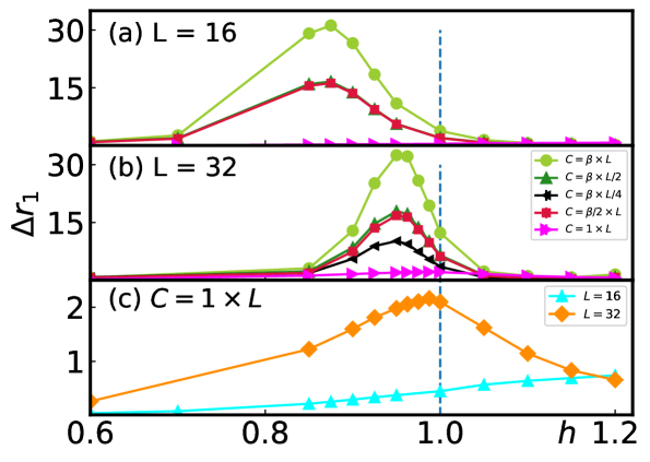
Figure 5: Quantum Ising model (statistics of NN distances for different system partitions). Panel (a): variance of the distribution function of the NN distances as a function of the transverse field for the complete data set of $L=16$ sites $\times$ $M^{\prime}=\beta=512$ slices (green circles), a spatial half-partition with the first $L/2$ sites and $\beta$ slices (dark green triangles), a temporal half-partition of the system with all $L$ sites but where only one every two of the original $M^{\prime}$ slices is considered (red squares), and a data set composed by a single slice for the complete system of $L$ sites (purple triangles). Panel (b): same as panel (a) for $L=32$, with the addition of the data set corresponding to a quarter-chain partition (i.e., the first $L/4=8$ sites) and all slices. Panel (c): magnification of the curves for the NN distance variance for single-slice data sets for $L=16,32$. In all panels, the vertical dashed line corresponds to the critical point $h=h_{c}$.

Regardless of the subset of degrees of freedom considered, in proximity of the critical point the observables display the same qualitative characteristics as their counterparts for the complete system, i.e., a peak for a size-dependent value of the transverse field. However, the details of such features, such as the height and position of the peak, depend on the number of degrees of freedom (sites $\times$ slices) considered: for instance, halving the number of degrees of freedom (either in space, by considering a half-chain partition, or in imaginary time, by considering only one slice every consecutive two) results in a roughly halved peak height, and the features are likewise much weaker in the case of single-slice calculations [but still present, see Fig. 5(c)]. This behavior shows essentially the same characteristics regardless of whether the “excised” degrees of freedom are spatial or temporal, suggesting an essentially equivalent role of the two in the calculation of $I_{d}$-related features.

Direct analysis of the features of $I_{d}$-related observables such as those displayed in, e.g., Fig. 4, points out that the strength of the $I_{d}$-related features (e.g., the height of the NN variance distribution peak) does not increase indefinitely with the addition of more degrees of freedom, but eventually reaches a size-independent saturation value corresponding to a complete system once a high enough number of temporal degrees of freedom is considered. It is also evident that, even for equivalent and large enough number of slices to reach the saturation threshold mentioned above, an $L$-sized partition of a larger system displays different features with respect to a full system of $L$ sites (as can be seen comparing the results for the $8\times M^{\prime}=512$ partition in Fig. 5 with those of the full $L=8$ system, and the same number of slices, in Fig. 4).

IV.2 Two-dimensional dimerized models

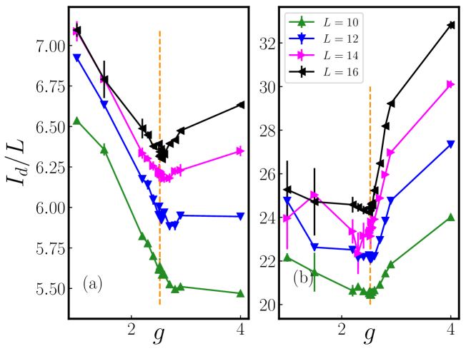
Figure 6: Heisenberg bilayer (intrinsic dimension). The graph shows the intrinsic dimension $I_{d}/L$ as a function of $g$ for different values of $L$. In panel (a) we consider data sets containing a single slice, while in panel (b) we consider ones with $\beta$ slices. For all results displayed here $\beta=L$. In all panels, the vertical dashed line corresponds to the critical point $g=g_{c}$.

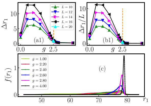
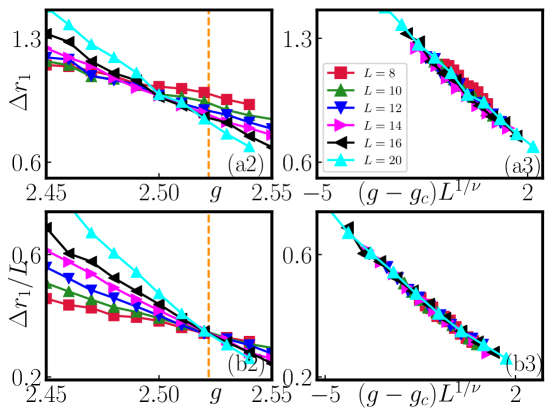
Figure 7: Heisenberg bilayer (statistics of NN distances). Panels (a1) and (a2) show the variance of the distribution function of the NN distances $f(r_{1})$, $\Delta r_{1}$, as a function of $g$ for single- and $\beta$-slices data sets, respectively; for the $\beta$-slices data set, we consider $\Delta r_{1}/L$ (see text). In panel (c), we show an example of $f(r_{1})$ for the $\beta$-slices data set and $L=10$. In panels (a2) and (b2) we present the blow-up of (a1) and (b1), respectively, in the region close to $g_{c}$. Finally, we show the data collapse of the results in panels (a3) and (b3). The value of $\nu$ is in agreement with the expected 3D Heisenberg universality class. For all results displayed here $\beta=L$. In all panels, the vertical dashed line corresponds to the critical point $g=g_{c}$.

We now consider the 2D dimerized Heisenberg bilayer model in Eq. (2). This Hamiltonian describes an AFM-paramagnetic transition belonging to the same universality class of the three-dimensional $O(3)$ Heisenberg model, see Sec. II.2.

Our simulations are performed using the SSE algorithm at inverse temperature $\beta=L$, an appropriate value for the investigation of the ground-state regime [47, 28]. For all the results discussed here, we consider data sets containing $N_{r}=5\times 10^{4}$ configurations. Furthermore, we consider configurations containing (i) single or (ii) a set of $M^{\prime}=\beta$ equally spaced slices. In order to ensure that the configurations belonging to the data set are uncorrelated, we computed the $I_{d}$ and $\Delta r_{1}$ of data sets generated by sampling configuration separated by $n_{AC}$ Monte Carlo steps, analyzing the dependence of the obtained estimates on the value of the latter. Our analysis resulted in the observation that, while our results depended strongly on the value of $n_{AC}$ for small inter-configuration distance, the values of $I_{d}$ and $\Delta r_{1}$ stabilized for $n_{AC}\gtrsim 10$, as expected once the decorrelated regime is reached. All results obtained via the SSE algorithm discussed here have been obtained following the procedure outlined above with $n_{AC}\geq 100$, ensuring the decorrelation of the analyzed configurations.

First, let us consider the behavior of the $I_{d}$. As in the case of the quantum Ising transition, the $I_{d}$ features a minimum close to the critical point $g_{c}$, which interestingly appears both for (i) single-slice [see Fig. 6(a)] and (ii) $\beta$-slices data sets [see Fig. 6(b)]. We note that the $I_{d}$ minimum position slightly changes when more slices are considered in the data set. In particular, for $\beta$-slices data sets and $L=16$, the minimum of the $I_{d}$ is located within $1\%$ of the QMC estimation of $g_{c}$ [43].

The analysis of the distribution of NN distances, $f(r_{1})$, provides further insight into the data structure emerging in the vicinity of $g_{c}$. The first striking observation is the non-monotonic behavior of the variance of $f(r_{1})$, $\Delta r_{1}$, for $g<g_{c}$, which displays a peak for $g\approx 0.5$ (interestingly, this is the same behavior observed for the AFM order parameter [42, 52]). This feature occurs for both the single- and $\beta$-slices data sets, which indicates that it is independent of the number of slices of the configurations; see Fig. 7(a1-b1). It is worth mentioning that this behavior is qualitatively different from the one observed for $\Delta r_{1}$ for the quantum Ising transition: in particular, here the position of the variance peak is (roughly) size-independent, and does not shift towards to the critical point. This difference is related to the underlying symmetries of these models - the SU($2$) of the Heisenberg bilayer and the $\mathbb{Z}_{2}$ of the quantum Ising model - and the corresponding symmetry-broken phases. Before explaining these results (see Sec. VI), which are of genuine quantum mechanical nature and pointing out the sharp difference between quantum and classical data sets, let us discuss the behavior of $\Delta r_{1}$ in the vicinity of $g_{c}$.

Indeed, we observe that $\Delta r_{1}$ ($\Delta r_{1}/L$) is (almost) a $L$-independent quantity close to $g_{c}$ when single-slice ($\beta$-slices) data sets are considered. The transition is then accurately identified by the crossing point of $\Delta r_{1}$ curves associated to different values of $L$, as illustrated in Fig. 7(a2-b2). In addition, Fig. 7(a3-b3) show that our results are well described by the FSS ansatz $\Delta r_{1}$ ($\Delta r_{1}/L$) $=f[(g-g_{c})L^{1/\nu}]$, where $\nu$ is the critical exponent associated to the divergence of the correlation length, for single-slice ($\beta$-slices) data sets. Our results are $g_{c}=2.50(2)$ and $\nu=0.71(2)$ ($g_{c}=2.52(1)$ and $\nu=0.68(2)$) for single slices ($\beta$-slices) data sets, differing of less than $1\%$ ($5\%$) from accurate estimations of these quantities based on FSS of physical observables [43].

Finally, it is worth mentioning that such a scaling behavior in the vicinity of 2D quantum critical points is also displayed by physical quantities including, e.g., the Binder moment ratios and the (rescaled) spin stiffness $L\rho_{s}$ [43]. Accurate estimations of critical points and exponents can be obtained with the same strategy adopted here, i.e, the detection of crossing points of results for different values of $L$. For example, one can determine the crossing points $g_{c}(L)$ for results corresponding to system sizes $L$ and $2L$, and then use FSS techniques to establish the value of $g_{c}(L\to\infty)$, which constitutes an estimate for the critical point. An interesting observation is that that the $g_{c}(L)$ associated to $\beta$-slices data sets converge faster to $g_{c}(L\to\infty)$ than the results for single-slice data sets, see Fig. 7(a2-b2). This is in line with what is observed in conventional FSS of physical quantities: i.e, the $g_{c}(L)$ associated with different observables exhibit different convergence to the $L\to\infty$ limit, as a consequence of subleading corrections of scaling functions. In this case, the crossing points associated with the spin stiffness exhibit the most rapid convergence to the thermodynamic limit [43]. Interestingly, $\rho_{s}$ is a non-equal-time quantity that depends on the full space-time structure of the path integral, which the $\beta$-slices data sets represent in the most faithful way.

To get further evidence for the conclusions described in this section, we also consider the Heisenberg columnar dimer model (see Appendix A). This Hamiltonian also describes a AFM-paramagnetic transition belonging to the same universality class of the three-dimensional $O(3)$ Heisenberg model. The results for the $I_{d}$ and $\Delta r_{1}$ are equivalent to the ones described above (see Fig. 13 in Appendix A), emphasizing how generic features of data structures are solely determined by the universal properties of the underlying quantum critical point.

V BKT transition

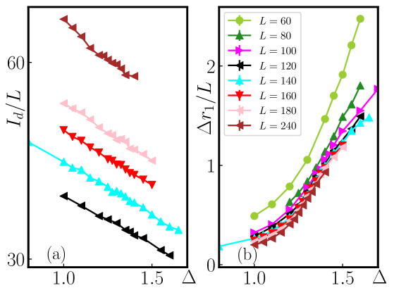
Figure 8: BKT transition - one-dimensional XXZ model. Results for single-slice data sets. Panel (a) and (b) display the $I_{d}$ and $\Delta r_{1}$, respectively, as a function of $\Delta$. For all results shown here $\beta=L$.

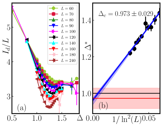
Figure 9: BKT transition - one-dimensional XXZ model. Results for the $\beta$-slices data sets. Panel (a) shows the intrinsic dimension, $I_{d}/L$, as a function of $\Delta$ for different values of $L$. In panel (b) we consider the finite-size scaling of the positions $\Delta^{*}(L)$ of the $I_{d}$ minima. The (blue) lines are line fittings performed with different sets of points, and the red horizontal line corresponds to the averaged $\Delta_{c}$ computed with such fittings. For all results displayed here $\beta=L$.

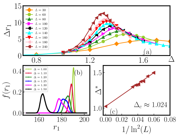
Figure 10: BKT transition - one-dimensional XXZ model. Results for the $\beta$-slices data sets. Panel (a) shows the variance of the distribution function of the NN distances $f(r_{1})$, $\Delta r_{1}$, as a function of $\Delta$ for different values of $L$. In panel (b), we show an example of $f(r_{1})$ for $L=140$ and different values of $\Delta$. Finally, in panel (c), we present the finite-size scaling of the positions $\Delta^{m}(L)$ of the maxima of $\Delta r_{1}$. For all results displayed here $\beta=L$.

In this section we consider the BKT transition described by the one-dimensional spin-$1/2$ XXZ model in Eq. (3). Differently from the cases discussed above, BKT quantum critical points (QCPs) are characterized by physical quantities associated to global properties of the full path integral configurations [44, 45, 3]. For instance, they are conventionally described by the spin stiffness, which is related to fluctuations of a topological property of path integral configurations (namely, the winding number). Nonlocal quantum-information quantities [53], and spectral properties [54, 55] are also used to pin down BKT QCPs.

The nature of BKT QCPs hints that successful unsupervised learning of such transitions relies (i) on the one hand, on defining a proper data set, that encompasses BKT topological properties, and (ii) on the other hand, on analyzing data set features that can reveal such global properties. Before discussing our results, let us mention that for the classical 2D XY model the $I_{d}$ exhibits signatures of the BKT phase transition [25]. Furthermore, dimensional reduction methods based on diffusion maps can detect the topological clustering structure of such classical data sets [33, 41]. Diffusion maps have also been used to reveal other topological properties (not related to BKT transitions) [37, 38, 15].

Let us now discuss how one can detect a BKT QCP with both the $I_{d}$ and $\Delta r_{1}$ by defining suitable path integral data sets. We employ the directed-loop SSE method to sample the path integral configurations, following the same protocol outlined in Sec. IV.2.

First, we consider the results associated with data sets containing single-slice configurations. In this case, we observe no particular feature in the behavior of either the $I_{d}$ or $\Delta r_{1}$ close to $\Delta_{c}=1$, see Fig. 8. Subsequently, we consider data sets formed by $\beta$-slices data sets. A fundamental technical aspect is that we retrieve slices separated by an interval of $\delta\tau\approx N_{s}$ in the SSE “imaginary-time” direction. Remarkably, in this case we observe that both the $I_{d}$ and $\Delta r_{1}$ exhibit singular features in the vicinity of $\Delta_{c}$, see Figs. 9 and 10.

More specifically, the $I_{d}$ features minima at size-dependent positions $\Delta^{*}(L)$ in the vicinity of $\Delta_{c}$. By performing a finite-size scaling of the minimum positions we obtain an estimate for the critical $\Delta_{c}$, see Fig. 9(b). Furthermore, we consider the data collapse of these results according to the FSS ansatz $I_{d}=L^{1-\omega}f(\xi/L)$, where the correlation length diverges as $\xi\sim\exp{(b/\sqrt{\Delta-\Delta_{c}})}$ [see Fig. 1(c)]. The value obtained for $\Delta_{c}$ via this procedure is in agreement with the exact one.

The statistics of NN distances $r_{1}$ also reveal the BKT quantum critical point. In particular, we note that the variance $\Delta r_{1}$ of the distribution $f(r_{1})$ exhibits a peak at size-dependent points $\Delta^{m}(L)$ in the vicinity of $\Delta_{c}$. The $\Delta^{m}(L)$ shifts towards $\Delta_{c}$ as $L\to\infty$, and their scaling to the thermodynamic limit allows to obtain an estimation of $\Delta_{c}$, see Fig. 10(b).

We also present the data collapse of our results using the FSS ansatz $\Delta r_{1}=L^{-\alpha}\tilde{f}(\xi/L)$ (Fig. 2). The quality of the collapse and the value obtained for $\Delta_{c}$ provides further numerical evidence that $\Delta r_{1}$ exhibits the universal scaling behavior characteristic of BKT QCPs.

Before concluding this section, let us mention about the influence of $\beta$ on our results. In our numerical simulations, we have found that as long as the value of $\beta$ is large enough to guarantee convergence to the ground state, the results for single-slice data sets are not affected by the choice of $\beta$. Oppositely, for the case of $\beta$-slices data sets, the values of $I_{d}$ and $\Delta r_{1}$ does depend on $\beta$, because the dimension of the embedding space changes with the latter; however, we observe that all the features associated to the phase transition of both $I_{d}$ (i.e., the minimum) and $\Delta r_{1}$ (i.e., the peak) do not change as $\beta$ increases (again, as long as $\beta$ is large enough to guarantee convergence to the ground state).

V.1 Discussion of the results

Summing up the results presented so far, we observe that both $I_{d}$ and $\Delta r_{1}$ exhibit singular features in the vicinity of both symmetry-breaking and BKT phase transitions.

Although we focus on paradigmatic models, we will now present arguments supporting the idea that these results are generic for the quantum data sets defined in Sec. II, and thus also apply for similar QCPs as the ones considered here. In previous work, some of us presented heuristic arguments to explain the relationship between the ID and the physical correlation length in classical phase transitions [25]. The basic idea lies in the hypothesis that the neighboring distances [see Eq. (14)] $r_{1}$ and $r_{2}$ are related to many-body correlations of the physical degrees of freedom of the system. This hypothesis can be straightforwardly applied to the quantum case for the specific setting in which the dynamical critical exponent satisfies $z=1$. In these cases, the intrinsic dimension is directly related to arbitrary rank correlation functions - and thus, shall display characteristic scaling behavior at the transition.

It is important to note that these arguments imply that $I_{d}$ and $\Delta r_{1}$ depend on correlations arising from both spatial and imaginary-time degrees of freedom. Our results indeed suggest that this is the case for $\beta$-slices data sets. For example, we mention the scaling of $I_{d}$ and $\Delta r_{1}$ for the TFIM shown in Figs. 3 and 4, which is analogous to physical quantities encompassing space-time degrees of freedom. Furthermore, in the case of BKT, we point out that single-slice data sets (encompassing solely spatial degrees of freedom) are insufficient to determine whether a transition exists at all, a fact which agrees with the topological nature of quantum BKT transitions.

VI Quantum data sets, symmetries, and symmetry-broken phases

So far we focused on the results emerging in the vicinity of different QCPs. We now argue that some of the data set features analyzed here can also reveal fundamental properties of symmetry-broken phases. In particular, let us review the behavior of $\Delta r_{1}$ in the different ordered phases encountered in this work: namely, (i) the $\mathbb{Z}_{2}$ ferromagnet described by the quantum Ising model, (ii) the Luttinger liquid and the $\mathbb{Z}_{2}$ antiferromagnet displayed in the 1D XXZ model, and (iii) the SU($2$) antiferromagnet described by the Heisenberg Bilayer.

Away from quantum critical points, we can summarize our results as follows: apart from the SU($2$) AFM case, $\Delta r_{1}$ is always an intensive (or weakly dependent on $L$) quantity, in both ordered and disordered phases. To illustrate this, in Fig. 11(b1-b2) we depict the scaling of the NN distance variance versus system size for the XXZ model. In the case of single-slice data sets (upper panel), the variance does not grow with $L$. In the $\beta$-slices case, the variance does not grow in the gapless phase, while in the AF phase it grows until it reaches the correlation length, and then starts decreasing (likely approaching a constant).

Opposite to this, in the SU($2$) AFM phase $\Delta r_{1}$ is an extensive quantity, i.e, $\Delta r_{1}\sim L$ (or $\Delta r_{1}/L\sim L$ for $\beta$-slices data sets). This behavior is depicted in Fig. 11(a1-a2). Below we argue that this result is related to the non-Abelian nature of the SU($2$)-symmetry-broken AFM phase, and reflects fundamental aspects of the quantum data sets.

The latter considered here are labeled by the value of commuting local observables (i.e., $z$ components of spin-$1/2$ degrees of freedom), while the full quantum state is characterized by the expectation values of non-commuting observables as well. An important aspect to consider is that one cannot measure simultaneously more than one local spin component (i.e., $S^{x}_{i}$, $S^{y}_{i}$, and $S^{z}_{i}$) in quantum data sets.

In order to show how this quantum aspect affects the results for $\Delta r_{1}$, we compare its scaling in the SU($2$) Heisenberg bilayer [see Fig. 7] with its classical counterpart, i.e., the classical O($3$) model. In the latter case, there is no problem in retaining a fully invariant SU(2) description, and we can define data sets formed by either (a) configurations $\vec{X}=(\vec{S}_{1},...,\vec{S}_{N_{s}}$), where $\vec{S}_{i}=(S^{x}_{i},S^{y}_{i},S^{z}_{i})$, and (b) configurations defined just by the $z$-components of the spins [i.e., $\vec{X}=(S^{z}_{1},...,S^{z}_{N_{s}})$], as in the quantum case.

In Fig. 12 we consider the temperature dependence of $\Delta r_{1}$ for the the classical O($3$) model. While for the data sets (a) $\Delta r_{1}$ exhibits a peak in the vicinity of the critical temperature $T_{c}$, for the data sets (b) $\Delta r_{1}$ sharply increases in the ordered phases (i.e., $T<T_{c}$). This reflects exactly what happens in the quantum case: when the full SU(2) symmetry is not resolved, the structure of the manifold changes drastically in symmetry-broken phases, and the variance of the distribution of distances increases extensively with system size. Note that the overall scale of $\Delta r_{1}$ is also very different: while the data sets (a) are embedded in a manifold that is three times as large (in terms of number of dimensions) as the (b) ones, $\Delta r_{1}$ at $L=10$ is an order of magnitude smaller in the symmetry-broken phase.

A qualitative explanation of the effect of SU(2) symmetry goes as follows: if a symmetry is not fully resolved, it is not possible to identify apparently different states as representatives of the same original state up to symmetric transformations, leading to artificially generated non-local correlations in the data sets, and to an enormously increased variance of distances. This effect becomes particularly evident in the case of symmetry breaking: the reason here is that clusters corresponding to different symmetry-broken regions are well separated, something that is not expected to happen in either critical or paramagnetic phases.

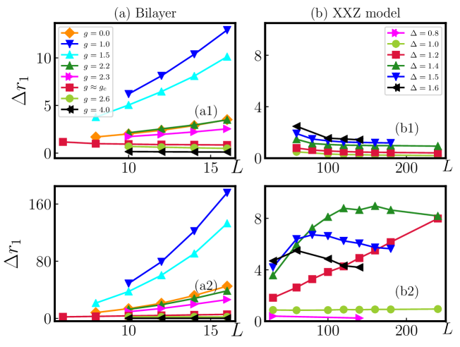
Figure 11: Size dependence of NN distance variance. Variance of the distribution function $f(r_{1})$, $\Delta r_{1}$, as function of the system size $L$. Panels (a) and (b) show our results for the 2D Heisenberg Bilayer and 1D XXZ models, respectively. In panels (a1) and (b1) we consider data sets generated by single-slice configurations, while in (a2) and (b2) we consider configurations containing $\beta$ slices. For all results displayed here $\beta=L$.

We can compare this picture with what happens when an Abelian symmetry is broken. The results for $\Delta r_{1}$ within the Ising FM phase (see Fig. 4) can also be compared with its classical counterpart, i.e., the two-dimensional Ising model (see ref. [25]). In this case, the classical data sets are defined exclusively in terms of $S^{z}$ variables, and in the FM phase $\Delta r_{1}$ exhibit analogous behavior to its quantum counterpart.

As a sanity check for the argument above, we can consider the critical point of the 1D Heisenberg model. Indeed, this point does not exhibit the extensive $\Delta r_{1}$ observed in its 2D counterpart. This difference shows that the extensive behavior of $\Delta r_{1}$ is indeed characteristic of the quantum fluctuations of the SU$(2)$-symmetry-broken phase, and not due the global symmetry of the system.

Our results thus directly indicate that the presence of non-Abelian symmetries can alter in a rather drastic manner the basic features of the PI manifold. This increased complexity of the data structure may be the origin of a recent set of observations in numerical studies using neural network ansatze as wave-functions. There, it was argued that neural network optimization may suffer significantly in the absence of a fully resolved symmetry. Our results are consistent with that observation, in that we provide evidence on why this happens: the underlying embedding manifold has artificial correlations introduced by the absence of symmetry resolution.

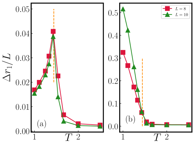
Figure 12: Classical Heisenberg model. Panels (a) and (b) show the variance of the distribution function of the NN distances $f(r_{1})$, $\Delta r_{1}$, as a function of $T$. In panel (a) we consider data sets generated by all $3$ spin components (i.e., $S^{x}$,$S^{y}$ and $S^{z}$), while in (b) we only consider the $S^{z}$ component (see text). In both panels, the vertical dashed line corresponds to the critical point, $T_{c}\approx 1.443$ [57].

VII Conclusions

We have shown how features of the raw data structure of partition functions reveal universal properties of both quantum phases and QCPs. The two key elements underlying our approach are (i) the introduction of a properly defined “raw data structure”, which is based on a proper treatment of space and imaginary-time degrees of freedom of path integral (or equivalently, stochastic-series-expansion) configurations generated by quantum Monte Carlo simulations; and (ii) the investigation of generic features of quantum data sets that are accessed without any dimensional reduction of the data set: namely, the intrinsic dimension, $I_{d}$, and the variance of the distribution of distances of NN configurations, $\Delta r_{1}$.

Our first key result is that both the $I_{d}$ and $\Delta r_{1}$ exhibit universal scaling behavior in the vicinity of both symmetry-breaking (i.e., related to the $\mathbb{Z}_{2}$ and the SU$(2)$ symmetries) and BKT QCPs. Data sets with a single imaginary-time slice are already enough to reveal symmetry-breaking QCPs at large enough system sizes. For the BKT transition, however, one needs to consider configurations containing a proper set of multiple slices. These results are traced back to the fact that while symmetry-breaking transitions are described by local order parameters, BKT QCPs take place due to topological changes of the full path integral configurations, and are associated with nonlocal correlations (encompassing both space and imaginary-time degrees of freedom). In this regard, our results elucidate the deep connection between generic properties of data sets - associated with the statistics of neighboring distances - and arbitrary-body correlations related to universal properties of quantum phase transitions. We note that $I_{d}$ is in general more reliable than $\Delta r_{1}$, as the latter might be sensitive to inhomogeneities in the data structure.

The second key observation is that the data structure of quantum partition functions simplifies (parametrically) as one approaches QCPs. Analogous conclusions are obtained for the conceptually simpler classical case [25]. This finding has a clear implications related to the complexity of (equilibrium) quantum states. While the intrinsic dimension is not a rigorously defined measure of complexity, it still provides a very informative, quantitative tool to witness it: a higher-dimensional manifold will always require a larger number of coordinates to be described. Our results show that quantum criticality leads to a drastic reduction in complexity in critical phases, that reflects the fact that the PI is very constrained due to universality. This witness of complexity behaves in a manner that is antipodal to entanglement, as the latter is typically growing close to criticality. It would be interesting to understand whether these two, apparently different, ways of addressing complexity can be directly compared: one possibility in this direction would be to apply our method to the transfer matrix corresponding to a fixed-bond-dimension tensor network.

Our third key observation is that the raw data structure of quantum partition functions is quantitatively affected by the spontaneous breaking of non-Abelian symmetries. In particular, we observe that the $\Delta r_{1}$ of data sets associated to the SU($2$) AFM phase exhibits dramatic differences compared to the Abelian cases considered here. Indeed, in the former case $\Delta r_{1}$ is an extensive quantity (i.e., $\Delta r_{1}\sim L$), while in the latter $\Delta r_{1}$ is almost independent of the system size (or even decreases with $L$). The explanation for this result is compatible with a key aspect of the quantum nature of the problem: namely, the SU($2$) non-Abelian symmetry cannot be fully resolved by data sets defined in terms of local spin measurements.

Let us conclude this paper by mentioning some perspectives for our work, by highlighting potential applications of the intrinsic dimension to other quantum mechanical objects.

One possible application concerns experiments. The first type of data set analyzed here (i.e., single-slice data sets) can be directly extracted via in situ imagining, at a similar cost to conventional correlation functions [16, 17, 18, 19, 20, 21, 22, 23, 58]. For example, one can consider the $I_{d}$ (or $\Delta r_{1}$) to witness complexity in a manner that is considerably less expensive to analyze than entanglement-related approaches, to detect phase transitions characterized by symmetry breaking, or even to reveal the presence of SU($2$) symmetry breaking from raw experimental data. We note that the number of realizations we typically consider here are in the order of $10^{4}/10^{5}$ configurations. While optical lattice experiments might face challenges in dealing with such statistics, other synthetic matter platforms such as Rydberg atoms in optical tweezers and trapped ions have already achieved these regimes thanks to, in large part, sub-Hz repetition rates. Solid state platforms are also capable of generating such large statistics.

Another possible future direction is to apply our approach to systems that suffer from the sign problem, to understand whether the latter reflects intrinsically onto the dimensionality of the data set [59, 60], or rather influences other geometrical properties (e.g., curvature). For instance, one may start by performing simulations in regimes where the sign problem is particularly mild (for instance, at high temperature), and track the complexity of the data structure as sampling becomes increasingly difficult. Another approach would be to extend the present method to Determinantal QMC based on auxiliary fields [34, 61, 62] or to adapt it to meron-type cluster techniques [63], in order to allow comparisons between different algorithms. Note that similar ideas might also be applied to other quantum mechanical objects, such as complex-valued Wigner functions.

Finally, let us mention possible connections of our work to recent efforts to define new classes of variational artificial-neural-network (ANN) quantum states. Physical data sets typically lay in a manifold whose $I_{d}$ is lower than the actual number of coordinates, as we extensively illustrate here. We believe that understanding the topography of such complex manifolds is the key to provide a data-based comprehension of ANN quantum states’ complexity. In this sense, the $I_{d}$ can provide an elementary tool for exploring the influence of the input data structure on learning ANN quantum states [64]. Unlike conventional variational approaches (e.g., based on tensor-network ansatze), where entanglement parametrizes complexity, ANN quantum states still lack a measure of the latter. The intrinsic dimension should be able, e.g., to give information about the number of ANN parameters (or layers) necessary to describe a given quantum state: for the particular case of autoencoders, we note that the intrinsic dimension is known to provide rigorous bounds on the functioning of the network depending on the dimension of its ’bottleneck’ layer. In this context, our analysis clearly shows that the dimensionality of the space could lead to a considerable simplification of the data structure: this clearly points to the fact that ANN (and, more specifically, autoencoders) could be particularly well suited to capture quantum criticality. Furthermore, within our framework, the importance of non-Abelian symmetries in shaping the data structure is particularly clear: not resolving such symmetries leads to a parametrically enhanced connectivity, that will likely affect the representative power of finite-depth ANN [65]. Going beyond these simple observations, our analysis may stimulate the investigation of whether other features of the path integral manifold, such as curvature or topology, are more challenging for ANN representations, and whether those could be of use to understand the relationship between ANN and tensor networks (see, e.g, Ref. [66, 67, 68]), both in the case of pure states, and in the case of mixed states. Similar considerations could be extended to ANN inspired by quantum field theory [69].

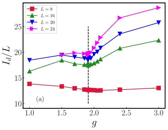
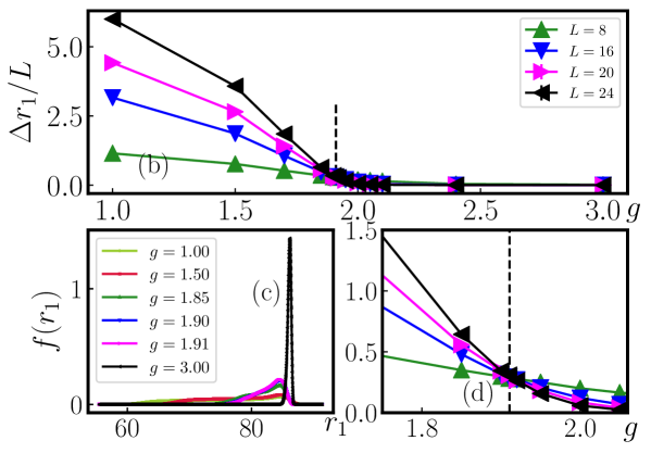
Figure 13: Heisenberg columnar dimer model. Panel (a): $I_{d}$ (rescaled with the system size) as a function of the coupling ratio $g$. Panel (b): rescaled variance of the NN distance distribution function, plotted as a function of $g$. Panel (c): NN distance distribution functions for selected values of $g$. Panel (d): magnification of the curve-crossing region of panel (b). For all data shown here, we considered $\beta$-slices configurations, with $\beta=L$. In all panels, the vertical dashed line corresponds to the critical point $g=g_{c}$.

VIII Acknowledgements

We acknowledge useful discussions with A. Browaeys, M. Heyl, A. Laio, R. T. Scalettar, and V. Vitale, and thank X. Turkeshi for collaboration on a related work. The work of AA, MD and TMS is partly supported by the ERC under grant number 758329 (AGEnTh), by the Quantera programme QTFLAG, by the MIUR Programme FARE (MEPH), and has received funding from the European Union’s Horizon 2020 research and innovation programme under grant agreement No 817482. This work has been carried out within the activities of TQT.

Appendix A 2D second-order transition: Heisenberg columnar dimer model

We now provide further evidence for the conclusions drawn in Secs. IV.2 and VI. An important aspect that we investigate is if our results are, indeed, solely determined by universal properties of the underlying QCP or if particular features of the system (e.g., the lattice geometry) can affect them. For example, for the bilayer geometry, one could argue that in the regime of almost decoupled layers (i.e., $g\ll 1$), uncorrelated DOF, in principle, may influence the behavior of data-based quantities. To address this issue, we consider a model describing an AFM-paramagnetic transition, but with a different lattice geometry than the bilayer: namely, the single-layer Heisenberg columnar dimer model [70, 71]

$$H=J\sum_{\langle i,j\rangle}\boldsymbol{S}_{i}\cdot\boldsymbol{S}_{j}+Jg\sum_{\langle i,j\rangle^{\prime}}\boldsymbol{S}_{i}\cdot\boldsymbol{S}_{j},$$ (16)

where $J$ and $Jg$ are exchange couplings constants defined on two set of bonds on a square lattice $\langle i,j\rangle$ and $\langle i,j\rangle^{\prime}$, respectively, following the notation of ref. [71]. In our simulations we set $J=1$. The ground-state properties of this model are equivalent to the bilayer Heisenberg model, i.e., it displays an $SU(2)$-symmetry-broken antiferromagnetic phase and an $SU(2)$-disordered phase for weak and strong values of $g$, respectively. QMC simulations show that the AFM-paramagnetic quantum phase transition takes place at $g_{c}=1.9096(2)$ [71], and belongs to the same universality class of the three-dimensional $O(3)$ Heisenberg model.

Our simulations are performed at inverse temperature $\beta=L$, and we consider $\beta$-slices data sets containing $N_{r}=5\times 10^{4}$ configurations.

In Fig. 13 we show the $I_{d}$ and the $\Delta r_{1}$ as function of $g$ for different system sizes $L$. Overall, our results confirm the conclusions drawn in Sec. IV.2 for the bilayer Heisenberg model. Indeed, in the vicinity of the QCP (i) the $I_{d}$ features a local minimum, and (ii) $\Delta r_{1}/L$ exhibits an (almost) $L$-independent behavior; the transition can then be identified (for sufficiently large system sizes) by the crossing point of $\Delta r_{1}/L$ curves for different values of $L$. These results highlight how universal properties of the underlying QCP solely determine generic features of data structures. Moreover, we observe that inside the $SU(2)$-symmetry-broken antiferromagnetic phase, $\Delta r_{1}/L$ exhibits an extensive behavior, confirming the important role of (broken) non-Abelian symmetries.

References

- Altland and Simons [2006] A. Altland and B. Simons, Condensed Matter Field Theory (Cambridge University Press, 2006).
- Montvay and Muenster [1994] I. Montvay and G. Muenster, Quantum Fields on a lattice (Cambridge Univ. Press, Cambridge, 1994).
- Sachdev [2000] S. Sachdev, Quantum Phase Transitions (Cambridge University Press, 2000).
- Calabrese and Cardy [2009a] P. Calabrese and J. Cardy, Entanglement entropy and conformal field theory, Journal of Physics A: Mathematical and Theoretical 42, 504005 (2009a).
- Amico et al. [2008] L. Amico, R. Fazio, A. Osterloh, and V. Vedral, Entanglement in many-body systems, Reviews of Modern Physics 80, 517 (2008).
- Lingua et al. [2019] F. Lingua, W. Wang, L. Shpani, and B. Capogrosso-Sansone, A topological signature of multipartite entanglement (2019), arXiv:1905.07454 .
- Facco et al. [2017] E. Facco, M. d’Errico, A. Rodriguez, and A. Laio, Estimating the intrinsic dimension of datasets by a minimal neighborhood information, Scientific Reports 7, 12140 (2017).
- Sandvik [2010] A. W. Sandvik, Computational studies of quantum spin systems, AIP Conference Proceedings 1297, 135 (2010), https://aip.scitation.org/doi/pdf/10.1063/1.3518900 .
- Krauth [1998] W. Krauth, Introduction to monte carlo algorithms, in Advances in Computer Simulation, edited by J. Kertész and I. Kondor (Springer Berlin Heidelberg, Berlin, Heidelberg, 1998) pp. 1–35.
- Lee et al. [2015] S. Lee, P. Campadelli, E. Casiraghi, C. Ceruti, and A. Rozza, Intrinsic dimension estimation: Relevant techniques and a benchmark framework, Mathematical Problems in Engineering (2015).
- Carleo and Troyer [2017] G. Carleo and M. Troyer, Solving the quantum many-body problem with artificial neural networks, Science 355, 602 (2017), https://science.sciencemag.org/content/355/6325/602.full.pdf .
- Carleo et al. [2019] G. Carleo, I. Cirac, K. Cranmer, L. Daudet, M. Schuld, N. Tishby, L. Vogt-Maranto, and L. Zdeborová, Machine learning and the physical sciences, Rev. Mod. Phys. 91, 045002 (2019).
- Carrasquilla [2020] J. Carrasquilla, Machine learning for quantum matter, Advances in Physics: X 5, 1797528 (2020), https://doi.org/10.1080/23746149.2020.1797528 .
- Cirac and Zoller [2012] J. I. Cirac and P. Zoller, Goals and opportunities in quantum simulation, Nature Physics 8, 264 (2012).
- Che et al. [2020] Y. Che, C. Gneiting, T. Liu, and F. Nori, Topological quantum phase transitions retrieved through unsupervised machine learning, Phys. Rev. B 102, 134213 (2020).
- Brydges et al. [2019] T. Brydges, A. Elben, P. Jurcevic, B. Vermersch, C. Maier, B. P. Lanyon, P. Zoller, R. Blatt, and C. F. Roos, Probing rényi entanglement entropy via randomized measurements, Science 364, 260 (2019).
- de Léséleuc et al. [2019] S. de Léséleuc, V. Lienhard, P. Scholl, D. Barredo, S. Weber, N. Lang, H. P. Büchler, T. Lahaye, and A. Browaeys, Observation of a symmetry-protected topological phase of interacting bosons with rydberg atoms, Science 365, 775 (2019).
- Chiaro et al. [2020] B. Chiaro, C. Neill, A. Bohrdt, M. Filippone, F. Arute, K. Arya, R. Babbush, D. Bacon, J. Bardin, R. Barends, S. Boixo, D. Buell, B. Burkett, Y. Chen, Z. Chen, R. Collins, A. Dunsworth, E. Farhi, A. Fowler, B. Foxen, C. Gidney, M. Giustina, M. Harrigan, T. Huang, S. Isakov, E. Jeffrey, Z. Jiang, D. Kafri, K. Kechedzhi, J. Kelly, P. Klimov, A. Korotkov, F. Kostritsa, D. Landhuis, E. Lucero, J. McClean, X. Mi, A. Megrant, M. Mohseni, J. Mutus, M. McEwen, O. Naaman, M. Neeley, M. Niu, A. Petukhov, C. Quintana, N. Rubin, D. Sank, K. Satzinger, A. Vainsencher, T. White, Z. Yao, P. Yeh, A. Zalcman, V. Smelyanskiy, H. Neven, S. Gopalakrishnan, D. Abanin, M. Knap, J. Martinis, and P. Roushan, Direct measurement of non-local interactions in the many-body localized phase (2020), arXiv:1910.06024 [cond-mat.dis-nn] .
- Pagano et al. [2020] G. Pagano, A. Bapat, P. Becker, K. S. Collins, A. De, P. W. Hess, H. B. Kaplan, A. Kyprianidis, W. L. Tan, C. Baldwin, and et al., Quantum approximate optimization of the long-range ising model with a trapped-ion quantum simulator, Proceedings of the National Academy of Sciences 117, 25396–25401 (2020).
- Scholl et al. [2020] P. Scholl, M. Schuler, H. J. Williams, A. A. Eberharter, D. Barredo, K.-N. Schymik, V. Lienhard, L.-P. Henry, T. C. Lang, T. Lahaye, A. M. Läuchli, and A. Browaeys, Programmable quantum simulation of 2d antiferromagnets with hundreds of rydberg atoms (2020), arXiv:2012.12268 [quant-ph] .
- Ebadi et al. [2020] S. Ebadi, T. T. Wang, H. Levine, A. Keesling, G. Semeghini, A. Omran, D. Bluvstein, R. Samajdar, H. Pichler, W. W. Ho, S. Choi, S. Sachdev, M. Greiner, V. Vuletic, and M. D. Lukin, Quantum phases of matter on a 256-atom programmable quantum simulator (2020), arXiv:2012.12281 [quant-ph] .
- Zeiher et al. [2017] J. Zeiher, J.-y. Choi, A. Rubio-Abadal, T. Pohl, R. van Bijnen, I. Bloch, and C. Gross, Coherent many-body spin dynamics in a long-range interacting ising chain, Physical Review X 7, 10.1103/physrevx.7.041063 (2017).
- Veit et al. [2021] C. Veit, N. Zuber, O. A. Herrera-Sancho, V. S. V. Anasuri, T. Schmid, F. Meinert, R. Löw, and T. Pfau, Pulsed ion microscope to probe quantum gases, Phys. Rev. X 11, 011036 (2021).
- Elben et al. [2020] A. Elben, R. Kueng, H.-Y. R. Huang, R. van Bijnen, C. Kokail, M. Dalmonte, P. Calabrese, B. Kraus, J. Preskill, P. Zoller, and B. Vermersch, Mixed-state entanglement from local randomized measurements, Physical Review Letters 125, 200501 (2020).
- Mendes-Santos et al. [2021] T. Mendes-Santos, X. Turkeshi, M. Dalmonte, and A. Rodriguez, Unsupervised learning universal critical behavior via the intrinsic dimension, Phys. Rev. X 11, 011040 (2021).
- Turkeshi [2021] X. Turkeshi, Measurement-induced criticality as a data-structure transition (2021), arXiv:2101.06245 [cond-mat.stat-mech] .
- Schmitt and Lenarčič [2021] M. Schmitt and Z. Lenarčič, From observations to complexity of quantum states via unsupervised learning (2021), arXiv:2102.11328 [quant-ph] .
- Sandvik [1997] A. W. Sandvik, An introduction to quantum monte carlo methods, in Strongly Correlated Magnetic and Superconducting Systems, Lecture Notes in Physics, edited by G. Sierra and M. A. Martin-Delgado (Springer, Berlin, Heidelberg, 1997) pp. 109–135.
- Becca and Sorella [2017] F. Becca and S. Sorella, Quantum Monte Carlo Approaches for Correlated Systems (Cambridge University Press, 2017).
- Calabrese and Cardy [2009b] P. Calabrese and J. Cardy, Entanglement entropy and conformal field theory, J. Phys. A: Math. Theor. 42, 504005 (2009b).
- Wang [2016] L. Wang, Discovering phase transitions with unsupervised learning, Phys. Rev. B 94, 195105 (2016).
- Hu et al. [2017] W. Hu, R. R. P. Singh, and R. T. Scalettar, Discovering phases, phase transitions, and crossovers through unsupervised machine learning: A critical examination, Phys. Rev. E 95, 062122 (2017).
- Rodriguez-Nieva and Scheurer [2019] J. F. Rodriguez-Nieva and M. S. Scheurer, Identifying topological order through unsupervised machine learning, Nature Physics 15, 790 (2019).
- Costa et al. [2017] N. C. Costa, W. Hu, Z. J. Bai, R. T. Scalettar, and R. R. P. Singh, Principal component analysis for fermionic critical points, Phys. Rev. B 96, 195138 (2017).
- Ch’ng et al. [2018] K. Ch’ng, N. Vazquez, and E. Khatami, Unsupervised machine learning account of magnetic transitions in the hubbard model, Phys. Rev. E 97, 013306 (2018).
- Canabarro et al. [2019] A. Canabarro, F. F. Fanchini, A. L. Malvezzi, R. Pereira, and R. Chaves, Unveiling phase transitions with machine learning, Phys. Rev. B 100, 045129 (2019).
- Long et al. [2020] Y. Long, J. Ren, and H. Chen, Unsupervised manifold clustering of topological phononics, Phys. Rev. Lett. 124, 185501 (2020).
- Lidiak and Gong [2020] A. Lidiak and Z. Gong, Unsupervised machine learning of quantum phase transitions using diffusion maps, Phys. Rev. Lett. 125, 225701 (2020).
- Hoan Tran et al. [2020] Q. Hoan Tran, M. Chen, and Y. Hasegawa, Topological persistence machine of phase transitions, arXiv e-prints , arXiv:2004.03169 (2020), arXiv:2004.03169 [cond-mat.stat-mech] .
- Kottmann et al. [2020] K. Kottmann, P. Huembeli, M. Lewenstein, and A. Acín, Unsupervised phase discovery with deep anomaly detection, Phys. Rev. Lett. 125, 170603 (2020).
- Wang et al. [2021] J. Wang, W. Zhang, T. Hua, and T.-C. Wei, Unsupervised learning of topological phase transitions using the calinski-harabaz index, Phys. Rev. Research 3, 013074 (2021).
- Sandvik and Scalapino [1994] A. W. Sandvik and D. J. Scalapino, Order-disorder transition in a two-layer quantum antiferromagnet, Phys. Rev. Lett. 72, 2777 (1994).
- Wang et al. [2006] L. Wang, K. S. D. Beach, and A. W. Sandvik, High-precision finite-size scaling analysis of the quantum-critical point of heisenberg antiferromagnetic bilayers, Phys. Rev. B 73, 014431 (2006).
- Gogolin et al. [2004] A. O. Gogolin, A. A. Nersesyan, and A. M. Tsvelik, Bosonization and Strongly Correlated Systems (Cambridge Univ. Press, Cambridge, 2004).
- Giamarchi [2004] T. Giamarchi, Quantum physics in one dimension, Internat. Ser. Mono. Phys. (Clarendon Press, Oxford, 2004).
- Wolff [1990] U. Wolff, Critical slowing down, Nuclear Physics B - Proceedings Supplements 17, 93 (1990).
- Sandvik and Kurkijärvi [1991] A. W. Sandvik and J. Kurkijärvi, Quantum monte carlo simulation method for spin systems, Phys. Rev. B 43, 5950 (1991).
- Sylju sen and Sandvik [2002] O. F. Sylju sen and A. W. Sandvik, Quantum monte carlo with directed loops, Phys. Rev. E 66, 046701 (2002).
- Sandvik [2019] A. W. Sandvik, Stochastic Series Expansion Methods, arXiv:1909.10591 [cond-mat] (2019), arXiv: 1909.10591.
- Levina and Bickel [2005] E. Levina and P. J. Bickel, Maximum likelihood estimation of intrinsic dimension, in Advances in Neural Information Processing Systems 17, edited by L. K. Saul, Y. Weiss, and L. Bottou (MIT Press, 2005) pp. 777–784.
- Pedregosa et al. [2011] F. Pedregosa, G. Varoquaux, A. Gramfort, V. Michel, B. Thirion, O. Grisel, M. Blondel, P. Prettenhofer, R. Weiss, V. Dubourg, J. Vanderplas, A. Passos, D. Cournapeau, M. Brucher, M. Perrot, and E. Duchesnay, Scikit-learn: Machine learning in Python, Journal of Machine Learning Research 12, 2825 (2011).
- Mendes-Santos et al. [2017] T. Mendes-Santos, N. C. Costa, G. Batrouni, N. Curro, R. R. dos Santos, T. Paiva, and R. T. Scalettar, Impurities near an antiferromagnetic-singlet quantum critical point, Phys. Rev. B 95, 054419 (2017).
- Rachel et al. [2012] S. Rachel, N. Laflorencie, H. F. Song, and K. Le Hur, Detecting quantum critical points using bipartite fluctuations, Phys. Rev. Lett. 108, 116401 (2012).
- Mishra et al. [2011] T. Mishra, J. Carrasquilla, and M. Rigol, Phase diagram of the half-filled one-dimensional -- model, Phys. Rev. B 84, 115135 (2011).
- Dalmonte et al. [2015] M. Dalmonte, J. Carrasquilla, L. Taddia, E. Ercolessi, and M. Rigol, Gap scaling at berezinskii-kosterlitz-thouless quantum critical points in one-dimensional hubbard and heisenberg models, Phys. Rev. B 91, 165136 (2015).
- Note [1] It is important to mention that strictly speaking the term “singular features” mean that a physical quantity (or some of its derivatives) diverges in the thermodynamic limit. In this work, although we do not show that and (or some of their derivatives) exhibit divergences, we employ the term “singular features”. This is motivated by our observation that such quantities exhibit scaling behavior close to quantum critical points. As occurs with singular physical quantities, this indicates that the correlation length dictates the behavior of and .
- Holm and Janke [1993] C. Holm and W. Janke, Finite-size scaling study of the three-dimensional classical Heisenberg model, Physics Letters A 173, 8 (1993), arXiv:hep-lat/9209017 [hep-lat] .
- Madjarov et al. [2020] I. S. Madjarov, J. P. Covey, A. L. Shaw, J. Choi, A. Kale, A. Cooper, H. Pichler, V. Schkolnik, J. R. Williams, and M. Endres, High-fidelity entanglement and detection of alkaline-earth rydberg atoms, Nature Physics 16, 857–861 (2020).
- Westerhout et al. [2020] T. Westerhout, N. Astrakhantsev, K. S. Tikhonov, M. I. Katsnelson, and A. A. Bagrov, Generalization properties of neural network approximations to frustrated magnet ground states, Nature Communications 11, 10.1038/s41467-020-15402-w (2020).
- Szabó and Castelnovo [2020] A. Szabó and C. Castelnovo, Neural network wave functions and the sign problem, Physical Review Research 2, 033075 (2020), arXiv:2002.04613 [cond-mat.str-el] .
- Broecker and Trebst [2016] P. Broecker and S. Trebst, Numerical stabilization of entanglement computation in auxiliary-field quantum monte carlo simulations of interacting many-fermion systems, Physical Review E 94, 10.1103/physreve.94.063306 (2016).
- Santos [2003] R. R. d. Santos, Introduction to quantum monte carlo simulations for fermionic systems, Braz. J. Phys. 33, 36 (2003).
- Chandrasekharan and Wiese [1999] S. Chandrasekharan and U.-J. Wiese, Meron-cluster solution of fermion sign problems, Phys. Rev. Lett. 83, 3116 (1999).
- Goldt et al. [2020] S. Goldt, M. Mézard, F. Krzakala, and L. Zdeborová, Modeling the influence of data structure on learning in neural networks: The hidden manifold model, Phys. Rev. X 10, 041044 (2020).
- Choo et al. [2019] K. Choo, T. Neupert, and G. Carleo, Two-dimensional frustrated model studied with neural network quantum states, Phys. Rev. B 100, 125124 (2019).
- Glasser et al. [2018] I. Glasser, N. Pancotti, M. August, I. D. Rodriguez, and J. I. Cirac, Neural-network quantum states, string-bond states, and chiral topological states, Physical Review X 8, 10.1103/physrevx.8.011006 (2018).
- Pastori et al. [2019] L. Pastori, R. Kaubruegger, and J. C. Budich, Generalized transfer matrix states from artificial neural networks, Physical Review B 99, 10.1103/physrevb.99.165123 (2019).
- Collura et al. [2021] M. Collura, L. Dell’Anna, T. Felser, and S. Montangero, On the descriptive power of neural-networks as constrained tensor networks with exponentially large bond dimension, SciPost Physics Core 4, 10.21468/scipostphyscore.4.1.001 (2021).
- Bachtis et al. [2021] D. Bachtis, G. Aarts, and B. Lucini, Quantum field-theoretic machine learning (2021), arXiv:2102.09449 [hep-lat] .
- Matsumoto et al. [2001] M. Matsumoto, C. Yasuda, S. Todo, and H. Takayama, Ground-state phase diagram of quantum heisenberg antiferromagnets on the anisotropic dimerized square lattice, Phys. Rev. B 65, 014407 (2001).
- Wenzel and Janke [2009] S. Wenzel and W. Janke, Comprehensive quantum monte carlo study of the quantum critical points in planar dimerized/quadrumerized heisenberg models, Phys. Rev. B 79, 014410 (2009).