Hypothesis Testing for Class-Conditional Label Noise

Abstract

In this paper we provide machine learning practitioners with tools to answer the question: is there class-conditional noise in my labels? In particular, we present hypothesis tests to check whether a given dataset of instance-label pairs has been corrupted with class-conditional label noise, as opposed to uniform label noise, with the former biasing learning, while the latter – under mild conditions – does not. The outcome of these tests can then be used in conjunction with other information to assess further steps. While previous works explore the direct estimation of the noise rates, this is known to be hard in practice and does not offer a real understanding of how trustworthy the estimates are. These methods typically require anchor points – examples whose true posterior is either $0$ or $1$. Differently, in this paper we assume we have access to a set of anchor points whose true posterior is approximately $1/2$. The proposed hypothesis tests are built upon the asymptotic properties of Maximum Likelihood Estimators for Logistic Regression models. We establish the main properties of the tests, including a theoretical and empirical analysis of the dependence of the power on the test on the training sample size, the number of anchor points, the difference of the noise rates and the use of relaxed anchors.

1 Introduction

When a machine learning practitioner is presented with a new dataset, a first question is that of data quality ([11]) as this will affect any subsequent tasks and inferences. This has led to tools to address transparency and accountability of data ([8, 23]). However, in supervised learning, an equally important concern is the quality of labels. For instance, in standard data collections, data curators usually rely on annotators from online platforms, where individual annotators cannot be unconditionally trusted as they have been shown to perform inconsistently ([10]). Labels are also expected to not be ideal in situations where the data is harvested directly from the web ([5], [21]). In general this is a product of annotations not being carried out by domain experts.

The existing literature focuses on estimating the distortion(s) present in the labels (see Section 4). In this paper we take a step back and our main contribution is the design and analysis of hypothesis testing procedures that would allow us (under certain assumptions we state later) to provide the practitioner with a measure of evidence for class-conditional noise, against uniform noise (as we discuss later, class-conditional noise biases the learning procedure, while uniform noise under mild conditions does not). With this information at hand, the practitioner can then make more informed decisions. What we present is designed to be performed after data collection and annotation to offer a quality measure with respect to label noise. If the quality is deemed poor, then the practitioner could resort to: (1) a modified data labelling procedure (e.g., active learning in the presence of noise), (2) seek methods to make the training robust (e.g., algorithms for learning from noisy labels), or (3) drop the dataset altogether.

In binary classification, the goal is to train a classifier $g:\mathcal{X}\to\{-1,+1\}$, from a labelled dataset $\mathcal{D}^{train}_{n}=\{(\boldsymbol{x}_{i},y_{i})\}_{i=1}^{n}\in(\mathbb{R}^{d}\times\{-1,1\})$, with the objective of achieving a low miss-classification error: $\mathbb{P}_{X,Y}(g(X)\neq Y)$. While it is generally assumed that the training dataset is drawn from the distribution for which we wish to minimise the error for $\mathcal{D}^{train}_{n}\sim p(X,Y)$, this is often not the case. Instead, the task requires us to train a classifier on a corrupted version of the dataset $\tilde{\mathcal{D}}^{train}_{n}\sim p(X,\tilde{Y})$ whilst still hoping to achieve a low error rate on the clean distribution. In this work we focus on one particular type of corruption: instance-independent label noise, where labels are flipped with a certain rate, that can either be uniform across the entire data-generating distribution or conditioned on the true class of the data point. A motivating example of class-conditional noise is given in [7] in the form of medical case-control studies, where different tests may be used for subject and control.

An essential ingredient in our procedure is the input from the user in the form of a set of anchor points. Differently from previous works, we assume anchor points for which the true posterior distribution $\mathbb{P}(Y=1\leavevmode\nobreak\ |\leavevmode\nobreak\ X=x)$ is (approximately) $\nicefrac{{1}}{{2}}$. For an instance $\boldsymbol{x}$ this requirement means that an expert would not be able to provide any help to identify the correct class label. While this will be shown to be convenient for theoretical purposes, finding such anchor points might be rather difficult to accomplish in practice, so we show how to relax this notion to a more realistic $\eta(x)\approx\nicefrac{{1}}{{2}}$. Anchor-points need to be provided by the experts.

Our approach is based on the asymptotic properties of the Maximum Likelihood Estimate (MLE) solution for Logistic Regression models, and the relationship between the true and noisy posteriors. On the theoretical side, we show that when the asymptotic properties of MLE hold and the user provides a single anchor point, we can devise hypothesis tests to assess the presence of class-conditional label corruption in the dataset. We then further extend these ideas to allow for richer sets of anchor points and illustrate how these lead to gains in the power of the test.

In Section 2 we cover the necessary background on MLE, noisy labels and define the necessary tools. In Section 3 we illustrate how to carry a $z$-test using anchor points on the presence of class-conditional noise. In Section 4 we discuss related work and in Section 5 we present experimental findings.

2 Background

We are provided with a dataset $(\boldsymbol{X},\boldsymbol{y})=\{(\boldsymbol{x}_{i},y_{i})\}_{i=1}^{N}\in(\mathbb{R}^{d}\times\{-1,1\})$, and our task is to assess whether the labels have been corrupted with class-conditional flipping noise. We use $y$ to denote the true label, and $\tilde{y}$ to denote the noisy label. We assume the feature vectors ($\boldsymbol{x}$) have been augmented with $ones$ such that we have $\boldsymbol{x}\to(1,\leavevmode\nobreak\ \boldsymbol{x})$. We assume the following model:

$$y_{i}\sim\text{Bernoulli}\left(\eta_{i}\right),\leavevmode\nobreak\ \leavevmode\nobreak\ \leavevmode\nobreak\ \leavevmode\nobreak\ \eta_{i}=\sigma(\theta_{0}^{\top}\boldsymbol{x}_{i})=\frac{1}{1+\exp\left(-\theta_{0}^{\top}\boldsymbol{x}_{i}\right)}$$

Following the MLE procedure we have: $\hat{\theta}_{n}:=\underset{\theta\in\Theta}{\operatorname{argmax}}\leavevmode\nobreak\ \ell_{n}\left(\theta\mid D_{n}\right)=\underset{\theta\in\Theta}{\operatorname{argmax}}\leavevmode\nobreak\ \prod_{i=1}^{n}\leavevmode\nobreak\ \ell_{i}\left(\theta\mid\boldsymbol{x}_{i},\leavevmode\nobreak\ y_{i}\right)$

where: $l\left(\theta\mid\boldsymbol{x}_{i},\leavevmode\nobreak\ y_{i}\right)=\frac{y_{i}+1}{2}\cdot\log\eta_{i}+\frac{1-y_{i}}{2}\cdot\log(1-\eta_{i})$. In this setting, the following can be shown (See for example Chapter 4 of [24]):

$$\sqrt{n}\left(\hat{\theta}_{n}-\theta_{0}\right)\leavevmode\nobreak\ \stackrel{{\scriptstyle D}}{{\longrightarrow}}\mathcal{N}\left(0,\leavevmode\nobreak\ I_{n}(\theta_{0})^{\raisebox{0.60275pt}{$\scriptscriptstyle-1$}}\right)$$ (1)

where $I_{\theta_{0}}$ denotes the Fisher-Information Matrix:

$$I_{n}(\theta_{0})=\mathbb{E}_{\theta}\left(-\frac{\partial^{2}\ell_{n}(\theta;Y\mid x)}{\partial\theta\partial\theta^{\top}}\right)=\mathbb{E}_{\theta}\left(-H_{n}(\theta;Y\mid x)\right)$$

where the expectation is with respect to the conditional distribution, and $H_{n}$ is the Hessian matrix.

We will consider two types of flipping noise and in both cases the noise rates are independent of the instance: $\mathbb{P}(\tilde{Y}=-i\leavevmode\nobreak\ |\leavevmode\nobreak\ Y=i,\leavevmode\nobreak\ X=x)=\mathbb{P}(\tilde{Y}=-i\leavevmode\nobreak\ |\leavevmode\nobreak\ Y=i)$ for $i\in\{-1,1\}$.

Definition 2.1.

Bounded Uniform Noise (UN)
In this setting the per-class noise rates are identical: $\mathbb{P}(\tilde{Y}=1\leavevmode\nobreak\ |\leavevmode\nobreak\ Y=-1)=\mathbb{P}(\tilde{Y}=-1\leavevmode\nobreak\ |\leavevmode\nobreak\ Y=1)=\tau$ and bounded: $\tau<0.50$. We will denote this setting with UN($\tau$), and a dataset $\mathcal{D}=(\boldsymbol{X},\boldsymbol{y})$ inflicted by UN($\tau$) by: $\mathcal{D}_{\tau}$.

Definition 2.2.

Bounded Class-Conditional Noise (CCN)
In this setting the per-class noise rates are different, $\alpha\neq\beta$ and bounded $\alpha+\beta<1$ with: $\mathbb{P}(\tilde{Y}=-1\leavevmode\nobreak\ |\leavevmode\nobreak\ Y=1)=\alpha$ and $\mathbb{P}(\tilde{Y}=1\leavevmode\nobreak\ |\leavevmode\nobreak\ Y=-1)=\beta$. We will denote this setting with CCN($\alpha,\beta$), and a dataset $\mathcal{D}=(\boldsymbol{X},\boldsymbol{y})$ inflicted by CCN($\alpha,\beta$) by: $\mathcal{D}_{\alpha,\beta}$.

An object of central interest in classification settings is the posterior predictive distribution: $\eta(\boldsymbol{x})=\mathbb{P}(Y=1\leavevmode\nobreak\ |\leavevmode\nobreak\ X=\boldsymbol{x})$. Its noisy counterpart, $\tilde{\eta}(\boldsymbol{x})\leavevmode\nobreak\ =\leavevmode\nobreak\ \mathbb{P}(\tilde{Y}=1\leavevmode\nobreak\ |\leavevmode\nobreak\ X=\boldsymbol{x})$, under the two settings, $UN(\tau)$ and $CCN(\alpha,\beta)$, can be expressed as: (See Appendix 8.1 for full derivation)

$$\tilde{\eta}(\boldsymbol{x})\leavevmode\nobreak\ =\left\{\begin{array}[]{ll}(1-\alpha-\beta)\cdot\eta(\boldsymbol{x})+\beta&\text{ if }\textrm{(CCN)}\\ (1-2\tau)\cdot\eta(\boldsymbol{x})+\tau&\text{ if }\textrm{(UN)}\\ \end{array}\right.$$ (2)

We consider loss functions that have the margin property: $\ell(y,f(x))=\psi(yf(x))$, where $f:\mathbb{R}^{d}\to\mathbb{R}$ is a scorer, and $g(\boldsymbol{x})=sign(f(\boldsymbol{x}))$ is the predictor. Let $f^{*}=\arg\min_{f\in\mathcal{F}}\leavevmode\nobreak\ \mathbb{E}_{X,Y}\psi(Yf(X))$ and $\tilde{f}^{*}=\arg\min_{f\in\mathcal{F}}\leavevmode\nobreak\ \mathbb{E}_{X,\tilde{Y}}\psi(\tilde{Y}f(X))$ denote the minimisers under the clean and noisy distributions, under model-class $\mathcal{F}$.

Definition 2.3.

Uniform Noise robustness ([9])
Empirical risk minimization under loss function $\ell$ is said to be noise-tolerant if $\mathbb{P}_{X,Y}(g^{*}(X)=Y)=\mathbb{P}_{X,Y}(\tilde{g}^{*}(X)=Y)$.

Theorem 2.1.

Sufficient conditions for robustness to uniform noise
Under uniform noise $\tau<0.50$, and a margin loss function, $\ell(y,f(x))=\psi(yf(x))$ satisfying: $\psi(f(X))+\psi(-f(X))=K$ for a positive constant $K$, we have that $\tilde{g}^{*}(x)=sign(\tilde{f}^{*}(x))$ obtained from: $\tilde{f}^{*}=\arg\min_{f\in\mathcal{F}}\leavevmode\nobreak\ \mathbb{E}_{X,\tilde{Y}}\psi(\tilde{Y}f(X))$ is robust to uniform noise.

For the proof see Appendix 8.2. Several loss functions satisfy this, such as: the square, unhinged (linear), logistic, and more. We now introduce our definition of anchor points.

Definition 2.4.

(Anchor Points) An instance $\boldsymbol{x}$ is called an anchor point if we are provided with its true posterior $\eta(\boldsymbol{x})$. Let $\mathcal{A}_{s}^{k}$ denote a collection of $k$ anchor points, with $\eta(\boldsymbol{x})=s\leavevmode\nobreak\ \forall\boldsymbol{x}\in\mathcal{A}_{s}^{k}$. Furthermore, let us also define $\mathcal{A}_{s,\delta}^{k}$, to imply that $\eta(\boldsymbol{x}_{i})=s+\epsilon_{i}$, for $\epsilon_{i}\sim\mathbb{U}([-\delta,\leavevmode\nobreak\ \delta])$, with $0\leq\delta\ll 1$ (respecting $0\leq\eta(\boldsymbol{x})\leq 1$). Also let $\mathcal{A}_{s,\delta}=\mathcal{A}_{s,\delta}^{1}$.

$$\mathcal{A}_{1}^{k}\leavevmode\nobreak\ \leavevmode\nobreak\ \leavevmode\nobreak\ \to\leavevmode\nobreak\ \leavevmode\nobreak\ \leavevmode\nobreak\ \eta(\boldsymbol{x})=1\leavevmode\nobreak\ \leavevmode\nobreak\ \leavevmode\nobreak\ \leavevmode\nobreak\ \leavevmode\nobreak\ \to\leavevmode\nobreak\ \leavevmode\nobreak\ \leavevmode\nobreak\ \tilde{\eta}(\boldsymbol{x})=1-\alpha$$

$$\mathcal{A}_{\nicefrac{{1}}{{2}}}^{k}\leavevmode\nobreak\ \leavevmode\nobreak\ \leavevmode\nobreak\ \to\leavevmode\nobreak\ \leavevmode\nobreak\ \leavevmode\nobreak\ \eta(\boldsymbol{x})=\nicefrac{{1}}{{2}}\leavevmode\nobreak\ \leavevmode\nobreak\ \leavevmode\nobreak\ \to\leavevmode\nobreak\ \leavevmode\nobreak\ \leavevmode\nobreak\ \tilde{\eta}(\boldsymbol{x})=\frac{1-\alpha+\beta}{2}$$

$$\mathcal{A}_{0}^{k}\leavevmode\nobreak\ \leavevmode\nobreak\ \leavevmode\nobreak\ \to\leavevmode\nobreak\ \leavevmode\nobreak\ \leavevmode\nobreak\ \eta(\boldsymbol{x})=0\leavevmode\nobreak\ \leavevmode\nobreak\ \leavevmode\nobreak\ \leavevmode\nobreak\ \leavevmode\nobreak\ \to\leavevmode\nobreak\ \leavevmode\nobreak\ \leavevmode\nobreak\ \tilde{\eta}(\boldsymbol{x})=\beta$$

The cases we will be referring to are shown to the right. The first and last, $\mathcal{A}_{1}^{k}$ and $\mathcal{A}_{0}^{k}$, have been used in the past in different scenarios. In this work we will make use of the second case, $\mathcal{A}_{\nicefrac{{1}}{{2}}}^{k}$.

3 Hypothesis Tests based on anchor points

In this section we introduce our framework for devising hypothesis tests to examine the presence of class-conditional label noise in a given dataset (with uniform noise, as the alternative), assuming we are provided with an anchor point(s). Our procedure is based on a two-sided z-test (see for example Chapter 8 of [1]) with a simple null hypothesis, and a composite alternative hypothesis (Eq.5). We first define the distribution under the null hypothesis (Eq.6), and under the alternative hypothesis (Eq.7), when provided with one strict anchor point ($\eta(x)=\nicefrac{{1}}{{2}}$). In this setting, for a fixed level of significance (Type I error) (Eq.8), we first derive a region for retaining the null hypothesis (Eq.9), and then we analyse the power (Prop.3.1) of the test (where we have that Type II Error = 1 - power). We then extend the approach to examine scenarios that include: (1) having multiple strict anchors ($\eta(x_{i})=\nicefrac{{1}}{{2}},\leavevmode\nobreak\ \forall i\in[k],\leavevmode\nobreak\ k>1$), (2) having multiple relaxed anchors ($\eta(x_{i})\approx\nicefrac{{1}}{{2}},\leavevmode\nobreak\ \forall i\in[k],\leavevmode\nobreak\ k>1$), and (3) having no anchors.

With the application of the delta method (See for example Chapter 3 of [24]) on Eq.1, we can get an asymptotic distribution for the predictive posterior:

$$\sqrt{n}(\hat{\eta}(\boldsymbol{x})-\eta(\boldsymbol{x}))\stackrel{{\scriptstyle D}}{{\longrightarrow}}\mathcal{N}\left(0,\leavevmode\nobreak\ [\eta(\boldsymbol{x})\{1-\eta(\boldsymbol{x})\}]^{2}\cdot\boldsymbol{x}^{\top}\boldsymbol{I}_{\theta_{0}}^{\raisebox{0.60275pt}{$\scriptscriptstyle-1$}}\boldsymbol{x}\right)$$ (3)

This fails in the case of $\eta(\boldsymbol{x})\in\{0,\leavevmode\nobreak\ 1\}$, so instead we work with $\nicefrac{{1}}{{2}}$. Which, together with the approximation of the Fisher-Information matrix with the empirical Hessian, we get:

$$\hat{\eta}(\boldsymbol{x})\stackrel{{\scriptstyle D}}{{\longrightarrow}}\mathcal{N}\left(\frac{1}{2},\leavevmode\nobreak\ \frac{1}{16}\cdot\boldsymbol{x}^{\top}\hat{H}_{n}\boldsymbol{x}\right)$$ (4)

where $\hat{H}_{n}=(X^{\top}DX)^{\raisebox{0.60275pt}{$\scriptscriptstyle-1$}}$, where $D$ is a diagonal matrix, with $D_{ii}=\hat{\eta}_{i}(1-\hat{\eta}_{i})$, where $\hat{\eta}_{i}=\sigma(\boldsymbol{x}_{i}^{\top}\hat{\theta})$.

For the settings: $(\mathcal{D},\leavevmode\nobreak\ \mathcal{A}_{\nicefrac{{1}}{{2}}}^{k})$ and $(\mathcal{D}_{\tau},\leavevmode\nobreak\ \mathcal{A}_{\nicefrac{{1}}{{2}}}^{k})$, for an $\boldsymbol{x}\in\mathcal{A}_{\nicefrac{{1}}{{2}}}^{k}$ we get: $\tilde{\eta}(\boldsymbol{x})=\frac{1}{2}$. While for $(\mathcal{D}_{\alpha,\beta},\leavevmode\nobreak\ \mathcal{A}_{\nicefrac{{1}}{{2}}}^{k})$ we get: $\tilde{\eta}(\boldsymbol{x})=\frac{1-\alpha+\beta}{2}$. Note that under $(\mathcal{D}_{\tau},\leavevmode\nobreak\ \mathcal{A}_{\nicefrac{{1}}{{2}}}^{k})$, we also have $[\tilde{\eta}(\boldsymbol{x})\{1-\tilde{\eta}(\boldsymbol{x})\}]^{2}=\frac{1}{16}$ similarly to $(\mathcal{D},\leavevmode\nobreak\ \mathcal{A}_{\nicefrac{{1}}{{2}}}^{k})$.

3.1 A Hypothesis Test for Class-Conditional Label Noise

We now define our null hypothesis ($\mathcal{H}_{0}$) and (implicit) alternative hypothesis ($\mathcal{H}_{1}$) as follows:

$$\mathcal{H}_{0}:\alpha=\beta\leavevmode\nobreak\ \leavevmode\nobreak\ \leavevmode\nobreak\ \leavevmode\nobreak\ \leavevmode\nobreak\ \&\leavevmode\nobreak\ \leavevmode\nobreak\ \leavevmode\nobreak\ \leavevmode\nobreak\ \leavevmode\nobreak\ \mathcal{H}_{1}:\alpha\neq\beta$$ (5)

Under the null and the alternative hypotheses, we have the following distributions for the estimated posterior of the anchor:

$$\mathcal{H}_{0}:\hat{\eta}(\boldsymbol{x}) \sim\mathcal{N}\left(\frac{1}{2},\leavevmode\nobreak\ \frac{1}{16}\cdot\boldsymbol{x}^{\top}\hat{H}\boldsymbol{x}\right)=\mathcal{N}\left(\frac{1}{2},\leavevmode\nobreak\ v(\boldsymbol{x})\right)$$ (6)

$$\mathcal{H}_{1}:\hat{\eta}(\boldsymbol{x}) \sim\mathcal{N}\left(\frac{1-\alpha+\beta}{2},\leavevmode\nobreak\ \frac{[(1-\alpha+\beta)(\beta-\alpha)]^{2}}{16}\cdot\boldsymbol{x}^{\top}\hat{\tilde{H}}\boldsymbol{x}\right)=\mathcal{N}\left(\frac{1+\alpha-\beta}{2},\leavevmode\nobreak\ \tilde{v}(\boldsymbol{x})\right)$$ (7)

Level of Significance and Power of the test

The level of significance (also known as Type I Error) is defined as follows:

$$a=\mathbb{P}(\textrm{reject}\leavevmode\nobreak\ \mathcal{H}_{0}\leavevmode\nobreak\ |\leavevmode\nobreak\ \mathcal{H}_{0}\leavevmode\nobreak\ \textrm{is True})$$ (8)

Rearranging Eq.6 we get: $\frac{\hat{\eta}(\boldsymbol{x})-\nicefrac{{1}}{{2}}}{\sqrt{v(\boldsymbol{x})}}\sim\mathcal{N}(0,\leavevmode\nobreak\ 1)$, under the null. Which for a chosen level of significance ($a$) allows us to define a region of retaining the null $\mathcal{H}_{0}$. We let $z_{\nicefrac{{a}}{{2}}}$ and $z_{1-\nicefrac{{a}}{{2}}}$ denote the lower and upper critical values for retaining the null at a level of significance of $a$.

Retain $\mathcal{H}_{0}$ if:

$$\leavevmode\nobreak\ z_{\nicefrac{{a}}{{2}}}\cdot\sqrt{v(x)}+\nicefrac{{1}}{{2}}\leavevmode\nobreak\ \leq\leavevmode\nobreak\ \leavevmode\nobreak\ \leavevmode\nobreak\ \leavevmode\nobreak\ \leavevmode\nobreak\ \leavevmode\nobreak\ \hat{\eta}(x)\leavevmode\nobreak\ \leavevmode\nobreak\ \leavevmode\nobreak\ \leavevmode\nobreak\ \leavevmode\nobreak\ \leq\leavevmode\nobreak\ z_{1-\nicefrac{{a}}{{2}}}\cdot\sqrt{v(x)}+\nicefrac{{1}}{{2}}$$ (9)

Using the region of retaining the null hypothesis, we can now derive the power of the test.

Proposition 3.1.

Power of the test (See Appendix 8.3 for the full derivation.)
Under the distributions for the estimated posterior under the null and alternative hypotheses in Eqs.6&7, based on the definition of the hypotheses in Eq.5, the test has power: $\mathbb{P}(\textrm{reject}\leavevmode\nobreak\ \mathcal{H}_{0}\leavevmode\nobreak\ |\leavevmode\nobreak\ \mathcal{H}_{0}\leavevmode\nobreak\ \textrm{is False})=1-b_{1}$, where:

$$b_{1}=\Phi\left(\frac{\displaystyle z\cdot\sqrt{v(x)}+\frac{\beta-\alpha}{2}}{\displaystyle\sqrt{\tilde{v}(x)}}\right)-\Phi\left(\frac{\displaystyle-z\cdot\sqrt{v(x)}+\frac{\beta-\alpha}{2}}{\displaystyle\sqrt{\tilde{v}(x)}}\right)$$ (10)

3.2 Multiple Anchor Points

Figure 1: Power of the hypothesis test as a function of $\beta-\alpha$, for a range of different $k$s. We set $v=(\nicefrac{{1}}{{16}})\cdot(X^{\top}DX)^{\raisebox{0.60275pt}{$\scriptscriptstyle-1$}}=0.1$.

In this section we discuss how the properties of the test change in the setting where multiple anchors points are provided.

Let $\hat{\eta}_{i}$ correspond to the $i$th instance in $\mathcal{A}_{\nicefrac{{1}}{{2}}}^{k}$. Then for $\bar{\eta}=\frac{1}{k}\sum_{i=1}^{k}\hat{\eta}_{i}$ we have:

$$\bar{\eta}\sim\mathcal{N}\left(\frac{1}{2},\leavevmode\nobreak\ \frac{1}{16}\cdot\bar{\boldsymbol{x}}^{\top}H\bar{\boldsymbol{x}}\right)$$

where $\bar{\boldsymbol{x}}=\frac{1}{k}\sum_{i=1}^{k}\boldsymbol{x}_{i}$ with $\boldsymbol{x}_{i}\in\mathcal{A}_{\nicefrac{{1}}{{2}}}^{k}\leavevmode\nobreak\ \forall i$. For the full derivation see Appendix 8.4.

Anchors chosen at random

We have that $\boldsymbol{x}\in\mathcal{A}_{\nicefrac{{1}}{{2}}}^{k}\to\boldsymbol{x}^{\top}\beta_{0}=0$, so that for an orthonormal basis $\boldsymbol{U}$, $\boldsymbol{x}=\boldsymbol{U}\boldsymbol{r}$. Without loss of generalisation we let $\boldsymbol{U}_{:,0}=\frac{\beta_{0}}{\|\beta_{0}\|_{2}}$, and therefore $\eta(x)=\nicefrac{{1}}{{2}}\to\boldsymbol{r}_{0}=0$. In words: $\forall\boldsymbol{x}\in\mathcal{A}_{\nicefrac{{1}}{{2}}}^{k}$ we have that $\boldsymbol{x}$’s component in the direction of $\beta_{0}$ is $0$.

Now we make the assumption that $\boldsymbol{x}$’s are random with $r_{j}\sim\mathbb{U}([-c,\leavevmode\nobreak\ c])$. Therefore, $\mathbb{E}r_{j}=0$, and $\mathbb{V}r_{j}=\frac{c^{2}}{3}$. In the following we use the subscript $S$ in the operator $\mathbb{E}_{S}$ to denote the randomness in choosing the set $\mathcal{A}$. In words: we assume that the set $\mathcal{A}_{\nicefrac{{1}}{{2}}}^{k}$ is chosen uniformly at random from the set of all anchor points.

Combining these we get:

$$\mathbb{E}_{S}v(x) =\mathbb{E}_{S}x^{\top}Hx=\mathbb{E}_{S}r^{\top}UHU^{\top}r$$

$$=\frac{dc^{2}}{3}\cdot tr(UHU^{\top})=\frac{dc^{2}q}{3}$$

where $q=tr(H)$. While for $k$ anchor points chosen independently at random, we get:

$$\mathbb{E}_{S}v(\bar{x})=\mathbb{E}_{S}\left[\frac{1}{k^{2}}\sum_{i,j}^{k}x_{i}^{\top}Hx_{j}\right]=\mathbb{E}_{S}\left[\frac{1}{k^{2}}\sum_{i,j}^{k}r_{i}^{\top}UHU^{\top}r_{j}\right]=\frac{dc^{2}}{3k}\cdot tr(UHU^{\top})=\frac{dc^{2}q}{3k}$$

Following the same derivation as above we get:

$$b_{k}=\Phi\left(\frac{\displaystyle z\cdot\sqrt{v(\bar{x})}+\frac{\beta-\alpha}{2}}{\displaystyle\sqrt{\tilde{v}(\bar{x})}}\right)\leavevmode\nobreak\ -\leavevmode\nobreak\ \Phi\left(\frac{\displaystyle-z\cdot\sqrt{v(\bar{x})}+\frac{\beta-\alpha}{2}}{\displaystyle\sqrt{\tilde{v}(\bar{x})}}\right)$$

If we let $v=\mathbb{E}_{S}v(x)$ (similarly $\tilde{v}=\mathbb{E}_{S}\tilde{v}(x)$), then we have seen that $\mathbb{E}_{S}v(\bar{x})=\frac{v}{k}$ (Reminder: expectations are with respect to the randomness in picking the anchor points). Then we have:

$$\frac{b_{k}}{b_{1}}=\frac{\displaystyle\Phi\left(\frac{z\sqrt{v}+h\sqrt{k}}{\sqrt{\tilde{v}}}\right)\leavevmode\nobreak\ -\leavevmode\nobreak\ \Phi\left(\frac{-z\sqrt{v}+h\sqrt{k}}{\sqrt{\tilde{v}}}\right)}{\displaystyle\Phi\left(\frac{z\sqrt{v}+h}{\sqrt{\tilde{v}}}\right)\leavevmode\nobreak\ -\leavevmode\nobreak\ \Phi\left(\frac{-z\sqrt{v}+h}{\sqrt{\tilde{v}}}\right)}\leavevmode\nobreak\ \leavevmode\nobreak\ \leq\leavevmode\nobreak\ \leavevmode\nobreak\ 1$$ (11)

with $h=\frac{\beta-\alpha}{2}$.

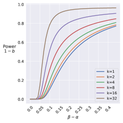
In Fig.1 we compare the power ($1-b$) of the test, as a function of the difference between the noise rates ($\beta-\alpha$), and number of anchor points used ($k$). We observe that a larger number of anchor points leads to a higher value for power.

3.3 Multiple Relaxed Anchors-Points

In this section we see how the properties of the test change in the setting where the anchors do not have a perfect $\eta(\boldsymbol{x})=\nicefrac{{1}}{{2}}$. We now consider the case of $\mathcal{A}_{\nicefrac{{1}}{{2}},\delta}^{k}$. Let $\boldsymbol{x}$ be such that $\eta(\boldsymbol{x})=\frac{1}{2}+\epsilon$, where $\epsilon\sim\mathbb{U}([-\delta,\delta])$ with $0<\delta\ll 1$. (Note: by definition $\delta\leq\nicefrac{{1}}{{2}}$.)

For one instance we have the following:  $\mathbb{E}_{\hat{\theta}}\hat{\eta}=\nicefrac{{1}}{{2}}+\epsilon,\leavevmode\nobreak\ \leavevmode\nobreak\ \leavevmode\nobreak\ \leavevmode\nobreak\ \text{and}\leavevmode\nobreak\ \leavevmode\nobreak\ \leavevmode\nobreak\ \leavevmode\nobreak\ \mathbb{E}_{S}\mathbb{E}_{\hat{\theta}}\hat{\eta}=\nicefrac{{1}}{{2}}$

For the variance component we have: $[\hat{\eta}(1-\hat{\eta})]^{2}=\left[\left(\frac{1}{2}+\epsilon\right)\left(\frac{1}{2}-\epsilon\right)\right]^{2}\approx\frac{1}{16}-\frac{\epsilon^{2}}{2}$, ignoring terms of order higher than $\epsilon^{2}$, under the assumption that $\delta\ll 1$.

Under the law of total variance we have:

$$\mathbb{V}(\eta) =\mathbb{E}\left(\mathbb{V}\left(\eta\leavevmode\nobreak\ |\leavevmode\nobreak\ \epsilon\right)\right)+\mathbb{V}\left(\mathbb{E}\left(\eta\leavevmode\nobreak\ |\leavevmode\nobreak\ \epsilon\right)\right)$$

$$=\mathbb{E}\left(\left(\frac{1}{16}-\frac{\epsilon^{2}}{2}\right)\cdot\boldsymbol{x}^{\top}H\boldsymbol{x}\right)+\mathbb{V}\left(\frac{1}{k}\sum_{i=1}^{k}\hat{\eta}_{i}\right)$$

$$=\left(\frac{1}{16}-\frac{\delta^{2}}{6}\right)\cdot\boldsymbol{x}^{\top}H\boldsymbol{x}+\mathbb{V}\left[\frac{1}{2}+\frac{1}{k}\sum_{i=1}^{k}\epsilon_{i}\right]$$

$$=\left(\frac{1}{16}-\frac{\delta^{2}}{6}\right)\cdot\boldsymbol{x}^{\top}H\boldsymbol{x}+\frac{\delta^{2}}{3k}$$ (12)

For the full derivation see Appendix 8.6. Finally, bringing everything together and ignoring $\delta^{2}$ terms we get:

$$\bar{\eta}\sim\mathcal{N}\left(\frac{1}{2},\leavevmode\nobreak\ \left(\frac{1}{16}-\frac{\delta^{2}}{6}\right)\cdot\bar{\boldsymbol{x}}^{\top}H\bar{\boldsymbol{x}}\right)\approx\mathcal{N}\left(\frac{1}{2},\leavevmode\nobreak\ \frac{1}{16}\cdot\bar{\boldsymbol{x}}^{\top}H\bar{\boldsymbol{x}}\right)$$

3.4 What if we have no anchor points?

We have shown that we can relax the hard constraint on the anchor points to be exactly $\eta=\nicefrac{{1}}{{2}}$, to $\eta\approx\nicefrac{{1}}{{2}}$. It is natural then to ask if we need anchor points at all. If instead we were to sample points at random, then we would have the following: $\mathbb{E}_{p(X)}\eta(X)=\pi$. The importance of needing for set of anchor points, either $\mathcal{A}_{\nicefrac{{1}}{{2}}}^{k}$ or $\mathcal{A}_{\nicefrac{{1}}{{2}},\delta}^{k}$, is that, the anchor points would be centered around a known value  $\nicefrac{{1}}{{2}}$ , as opposed to having no anchor points and sampling at random, where the anchor points would end up being centered around $\pi$. Knowledge of the class priors could allow for a different type of hypothesis tests to asses the presence of label noise. We do not continue this discussion in the main document as it relies on different type of information, but provide pointers in the Appendix 8.8.

3.5 Practical Considerations & Limitations

Beyond Logistic Regression

Our approach relies on the asymptotic properties of MLE estimators, and specifically of Logistic Regression. More complex models can be constructed in a similar fashion through polynomial feature expansion. However the extension of these tests to richer model-classes, such as Gaussian Processes, remains open.

Multi-class classification

Multi-class classification setting can be reduced to one-vs-all, all-vs-all, or more general error-correcting output codes setups as described in [4], which rely on multiple runs of binary classification. In these settings then we could apply the proposed framework. The challenge would then be how to interpret $\eta=\nicefrac{{1}}{{2}}$.

Finding anchor points

While it might not be straightforward for the user to provide instances whose true posterior is $\eta(\boldsymbol{x})=\nicefrac{{1}}{{2}}$, we do show how this can be relaxed, by allowing $\eta(\boldsymbol{x})\approx\nicefrac{{1}}{{2}}$. We then show how multiple anchor points can be stacked, improving the properties of the test.

Model Misspecification

Our work relies on properties of the MLE and its asymptotic distribution (Eq. 1). These assume the model is exactly correct. Similarly, under the null in the scenario of $\alpha=\beta>0$, we are at risk of model misspecification. This is not a new problem for Maximum Likelihood estimators, and one remedy is the so-called Huber Sandwich Estimator [6] which replaces the Fisher Information Matrix, with a more robust alternative.

Instance-dependent Noise (IDN)

In IDN the probability of label flipping depends on the features. It can be seen as a generalisation over UN (which is unbiased under mild conditions (See Theorem 2.1) and CCN (where learning is in general biased). Our theoretical framework for CCN serves as a starting point to devise tests of IDN. One potential way of extending our approach to test for IDN could be to have anchor points at different contours, i.e., 0.20, 0.30, … 0.70.

4 Related Work

There exist multiple works in the field of weak supervision where instead of being provided with the true labels, the dataset is annotated with a weak version of them, usually derived from the true label and potentially influenced by exogenous variables. It is beyond the scope of this work to discuss this field but these works and the references therein offer an overview of the field: [16, 13, 3, 18, 7].

We briefly discuss approaches in the literature that relate to tackling the problem of learning with the presence of (flipping) noise in the labels. As already discussed in Theorem 2.1, in the case of uniform noise, under mild assumptions, we have robust risk minimisation. However, in the case of class-conditional noise, we do not have similar guarantees.

One common approach is to proceed by correcting the loss to be minimised, by introducing the mixing matrix $\boldsymbol{M}\in[0,1]^{c\times c}$, where $M_{i,j}=\mathbb{P}(\tilde{y}=\boldsymbol{e}^{j}\leavevmode\nobreak\ |\leavevmode\nobreak\ y=\boldsymbol{e}^{i})$ [16].

Anchor points and perfect samples

Using these formulations, we are in a position where, if we have access to $\boldsymbol{M}$, we can correct the training procedure to obtain an unbiased estimator. However, $\boldsymbol{M}$ is rarely known and is difficult to estimate. Works on estimating $\boldsymbol{M}$ rely on having access to ‘perfect samples’ and can be traced back to [22], and the idea was later adapted and generalised in [16, 13, 12, 19] to the multi-class setting. Interestingly, in [17] authors do not explicitly define these perfect samples, but rather assume they do exist in a large enough (validation) dataset $\boldsymbol{X}^{\prime}$ - obtaining good experimental results. Similarly, [25] also work by not explicitly requiring anchor points, but rather assuming their existence.

Noisy examples

An alternative line is followed by [15, 14], where the aim is to identify the specific examples that have been inflicted with noise. This is a non-trivial task unless certain assumptions can be made about the per-class distributions, and their shape. For example, if we can assume that the supports of the two classes do not overlap (i.e. $\eta(x)(1-\eta(x))\in\{0,1\}\leavevmode\nobreak\ \forall x$), then we can identify mislabelled instances using per-class densities. If this is not the case, then it would be difficult to differentiate between a mislabelled instance and an instance for which $\eta(x)(1-\eta(x))\in(0,1)$. A different assumption could be uni-modality, which would again provide a prescription for identifying mislabelled instances through density estimation tools.

Distilled examples

The authors in [2] go in the opposite direction by trying to identify instances that have not been corrupted $\to$ the distilled examples. As a first step the authors assume knowledge of an upper-bound (Theorem 2 of [2]) which allows them to define sufficient conditions for identifying whether an instance is clean. As a second step they aim at estimating the (local) noise rate based on the neighbourhood of an instance (Theorem 3 of [2]).

Informative priors

Bayesian Statistics is often concerned with constructing informative prior distributions that reflect expert knowledge. While it might be challenging eliciting information from experts and modeling it quantitatively; it is often a necessary, and useful, step in low-data settings.

Similarly to the first set of works we introduce and exploit anchor points, but not for directly estimating the mixing matrix, but rather to devise hypothesis tests to obtain evidence against the null hypothesis: the dataset having been inflicted with uniform noise, as opposed to class-conditional uniform noise.

5 Experiments

In order to illustrate the properties of the tests, for the experiments we consider a synthetic dataset where the per-class distributions are Gaussians, with means $[1,\leavevmode\nobreak\ 1]^{\top}$ and $[-1,\leavevmode\nobreak\ -1]^{\top}$, with identity as scale. For this setup we know that anchor points should lie on the line $y=-x$, and draw them uniformly at random $x\in[-4,\leavevmode\nobreak\ 4]$. We analyse the following parameters of interest:

1. $N\in[500,\leavevmode\nobreak\ 1000,\leavevmode\nobreak\ 2000,\leavevmode\nobreak\ 5000]$: the training sample size.

2. $(\alpha-\beta)\in[-0.05,\leavevmode\nobreak\ 0.10,\leavevmode\nobreak\ 0.20]$: the difference between the per-class noise rates.

3. $k\in[1,\leavevmode\nobreak\ 2,\leavevmode\nobreak\ 4,\leavevmode\nobreak\ 8,\leavevmode\nobreak\ 16,\leavevmode\nobreak\ 32]$: the number of anchor points.

4. $\delta\in[0,\leavevmode\nobreak\ 0.05,\leavevmode\nobreak\ 0.10]$: how relaxed the anchor points are: $\eta(x)\in[0.50-\delta,\leavevmode\nobreak\ 0.50+\delta]$.

For all combinations of $N$ and $(\alpha-\beta)$ we perform $500$ runs. In each run, we generate a clean version of the data $\mathcal{D}$, and then proceed by corrupting it to obtain a separate version: $\mathcal{D}_{\alpha,\beta}$. For both datasets, we fit a Logistic Regression model. We sample both the anchor points and relaxed anchor points. Finally, we then compute the z-scores, and subsequently the corresponding p-values.

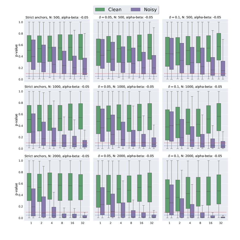
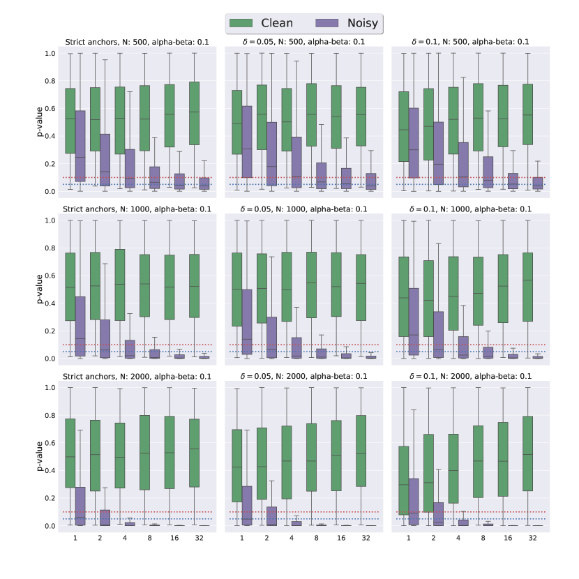
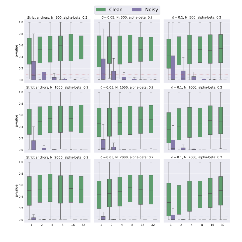
The box-plots should be read as follows: $Q1,\leavevmode\nobreak\ Q2\leavevmode\nobreak\ \&\leavevmode\nobreak\ Q3$ separate the data into $4$ equal parts. The inner box starts (at the bottom) at $Q1$ and ends (at the top) at $Q3$, with the horizontal line inside denoting the median ($Q2$). The whiskers extend to show $Q1-1.5\cdot IQR$, and $Q3+1.5\cdot IQR$. $IQR$ denotes the Interquartile Range and $IQR=Q3-Q1$.

In Figures 3, 3 and 4 we have the following: moving to the right we increase the relaxation of anchor points, and moving downwards we increase the training sample-size. On the subplot level, on the x-axis we vary the number of anchor points, and on the y-axis we have the p-values. In all subplots we indicate with a red dashed line the mark of $0.10$, and with a blue one the mark of $0.05$, which would serve as rejection thresholds for the null hypothesis.

The experiments are illustrative of the claims made earlier in the paper. Below we discuss the findings in the experiments and what they mean with regards to Type I and Type II errors. We discuss these points in two parts; we first discuss the effect on sample size ($N$), difference in noise rates ($|\alpha-\beta|$) and number of anchor points ($k$).

Size of training set ($N$)

As the size of training set ($N$) increases, the power increases. This can be seen Figures 3, 3 & 4. By moving down the first column, and fixing a value for $k$, where $N$ increases, we see the range of the purple box-plots decreasing, and essentially a larger volume of tests falling under the cut-off levels of significance (red and blue dashed lines). This is expected given that the variance of the MLE $\hat{\theta}_{MLE}$ vanishes as $N$ increases, as is seen in Eq.1 and discussion underneath it.

Difference in noise rates ($|\alpha-\beta|$)

As $|\alpha-\beta|$ increases, the power increases. This can be seen in Figures 3, 3 & 4, by fixing a particular subplot in the first column (for example, top-left one), and a value for $k$, we see again that the volume moves down. As presented in Eq.10, as $\beta-\alpha$ increases, the power also increases.

Number of anchor points ($k$)

The same applies to the number of anchor points – as the number of anchor points ($k$) increases, the power of the test increases. This can be seen in all three figures by focusing in any subplot in the first column, and considering the purple box-plots moving to the right. In Eq.11 we see effect of $k$ on the power.

In all three discussions above we focused on the first column of each of the figures – which shows results from experiments on strict anchors. What we also observe in this case (the first column of all figures) is that the p-values follow the uniform distribution under the null (as expected, given the null hypothesis is true) – shown by the green box-plots. Therefore the portion of Type I Errors = $a$ (the level of significance Eq.8). When we relax the requirements for strict anchors to allow for values close to $\nicefrac{{1}}{{2}}$, we introduce a bias in the lower and upper bounds in Eq.9 of $+\epsilon$. While $\mathbb{E}\epsilon=0$ this shift on the boundaries of the retention region will increase Type I Error. On the other hand, in Eq.12 we see how this bias decreases as you increase the number of anchor points. Both of these phenomena are also shown experimentally by looking at the latter two columns of the figures.

Anchor point relaxation ($\delta$)

Lastly, we examine the effect of relaxing the strictness of the anchors ($\delta$), $\eta(x)\in[0.50-\delta,\leavevmode\nobreak\ 0.50+\delta]$ on the properties of the test. As just discussed we see that as we increase the number of anchor points Type I Error decreases (volume of green box-plots under each of the cut-off points). We also observe that, as compared to only allowing strict anchors, the power is not affected significantly – with the effect decreasing as the number of anchor points increases. Furthermore, in the latter two columns we also observe the phenomena mentioned in the discussion concerning the first column only.

Figure 2: Box-plots with fixed $|\beta-\alpha|=0.05$. Red dotted line indicates the mark of $0.10$, and the blue one $0.05$.

Figure 3: Box-plots with fixed $|\beta-\alpha|=0.10$. Red dotted line indicates the mark of $0.10$, and the blue one $0.05$.

Figure 4: Box-plots with fixed $|\beta-\alpha|=0.20$. Red dotted line indicates the mark of $0.10$, and the blue one $0.05$.

6 Conclusion & Future Work

In this work we introduce the first statistical hypothesis test for class-conditional label noise. Our approach requires the specification of anchor points, i.e. instances whose labels are highly uncertain under the true posterior probability distribution, and we show that the test’s significance and power is preserved over several relaxations on the requirements for these anchor points.

Our experimental analysis, which confirms the soundness of our test, explores many configurations of practical interest for practitioners using this test. Of particular importance for practitioners, since anchor specification is under their control, is the high correspondence shown theoretically and experimentally between the number of anchors and test significance.

Future work will cover both theoretical and experimental components. On the theoretical front, we are interested in understanding the test’s value under a richer set of classification models, and further relaxing requirements on true posterior uncertainty for anchor points. Experimentally, we are particularly interested in applying the tests to diagnostically challenging healthcare problems and utilising clinical experts for anchor specification.

7 Appendix

7.1 Derivation of the Noisy Posterior

We can compute the noisy posterior: $\tilde{\eta}(x)=\mathbb{P}(\tilde{y}=1\leavevmode\nobreak\ |\leavevmode\nobreak\ X=x)$ as follows:

$$\tilde{\eta}(x)\leavevmode\nobreak\ =\leavevmode\nobreak\ \mathbb{P}(\tilde{y}=1,\leavevmode\nobreak\ y=1\leavevmode\nobreak\ |\leavevmode\nobreak\ X=x)$$

$$\leavevmode\nobreak\ \leavevmode\nobreak\ \leavevmode\nobreak\ \leavevmode\nobreak\ \leavevmode\nobreak\ \leavevmode\nobreak\ \leavevmode\nobreak\ \leavevmode\nobreak\ +\leavevmode\nobreak\ \mathbb{P}(\tilde{y}=1,\leavevmode\nobreak\ y=0\leavevmode\nobreak\ |\leavevmode\nobreak\ X=x)$$

$$=\leavevmode\nobreak\ \mathbb{P}(\tilde{y}=1\leavevmode\nobreak\ |\leavevmode\nobreak\ y=1)\mathbb{P}(y=1\leavevmode\nobreak\ |\leavevmode\nobreak\ X=x)$$

$$\leavevmode\nobreak\ \leavevmode\nobreak\ \leavevmode\nobreak\ \leavevmode\nobreak\ \leavevmode\nobreak\ \leavevmode\nobreak\ \leavevmode\nobreak\ \leavevmode\nobreak\ +\leavevmode\nobreak\ \mathbb{P}(\tilde{y}=1\leavevmode\nobreak\ |\leavevmode\nobreak\ y=0)\mathbb{P}(y=0\leavevmode\nobreak\ |\leavevmode\nobreak\ X=x)$$

$$=\leavevmode\nobreak\ (1-\alpha)\cdot\eta(x)+\beta\cdot(1-\eta(x))$$

$$=\leavevmode\nobreak\ \left\{\begin{array}[]{ll}(1-\alpha-\beta)\cdot\eta(\boldsymbol{x})+\beta&\text{ if }\textrm{(CCN)}\\ (1-2\tau)\cdot\eta(\boldsymbol{x})+\tau&\text{ if }\textrm{(UN)}\end{array}\right.$$ (15)

7.2 Sufficient conditions for robustness to uniform noise

In the case of uniform-noise we have that:

$$sign(\tilde{\eta}(x)-0.50)\leavevmode\nobreak\ =\leavevmode\nobreak\ sign((1-2\tau)\cdot(\eta(x)-0.50))$$

$$=\leavevmode\nobreak\ sign(\eta(x)-0.50)$$

where the last equality holds under the assumptions in Def. 2.1.

$$\mathbb{E}_{X,Y}l(Y,f(X))=\mathbb{E}_{X}\mathbb{E}_{Y|X}l(Y,f(X))=\mathbb{E}_{X}\mathbb{E}_{Y|X}\psi(Yf(X))$$

but we have access to noisy versions of labels

$$\mathbb{E}_{X}\mathbb{E}_{\tilde{Y}|X}\psi(\tilde{Y}f(X))$$

$$=\mathbb{E}_{X}\Big{[}\tilde{\eta}\cdot\psi(f(X))+(1-\tilde{\eta})\cdot\psi(-f(X))\Big{]}$$

$$=\mathbb{E}_{X}\Big{[}[(1-\tau)\eta+\tau(1-\eta)]\cdot\psi(f(X))$$

$$\leavevmode\nobreak\ \leavevmode\nobreak\ \leavevmode\nobreak\ \leavevmode\nobreak\ \leavevmode\nobreak\ +[(1-\tau)(1-\eta)+\tau\eta]\cdot\psi(-f(X))\Big{]}$$

$$=\mathbb{E}_{X}\Big{[}(1-2\tau)\cdot\mathbb{E}_{Y|X}\psi(Yf(X))$$

$$\leavevmode\nobreak\ \leavevmode\nobreak\ \leavevmode\nobreak\ \leavevmode\nobreak\ \leavevmode\nobreak\ +\tau\cdot[\psi(f(X))+\psi(-f(X))]\Big{]}$$

$$=(1-2\tau)\cdot\mathbb{E}_{X,Y}l(Y,f(X))+\tau\cdot BIAS_{\tau}(\psi)$$

This implies that if we train under uniform-noise with rate: $\tau<0.50$, with a loss with the property that $\psi(f(X))+\psi(-f(X))=K$ for a constant $K$ then risk minimisation is tolerant to noise [9].

7.3 Derivation for proposition 3.1

We let $L$ and $U$ denote the lower and upper bounds in Eq.9 respectively, and let $\epsilon\sim\mathcal{N}(0,\leavevmode\nobreak\ 1)$.

$$b_{1} \leavevmode\nobreak\ =\mathbb{P}(\textrm{retain}\leavevmode\nobreak\ \mathcal{H}_{0}\leavevmode\nobreak\ |\leavevmode\nobreak\ \mathcal{H}_{0}\leavevmode\nobreak\ \textrm{is False})$$

$$\leavevmode\nobreak\ =\mathbb{P}\left(L\leq\hat{\eta}(x)\leq U\leavevmode\nobreak\ |\leavevmode\nobreak\ \hat{\eta}(x)\sim\mathcal{N}\left(\frac{1+\alpha-\beta}{2},\leavevmode\nobreak\ \tilde{v}(x)\right)\right)$$

$$\leavevmode\nobreak\ =\mathbb{P}\left(L\leq\hat{\eta}(x)\leq U\leavevmode\nobreak\ |\leavevmode\nobreak\ \hat{\eta}(x)=\frac{1+\alpha-\beta}{2}+\sqrt{\tilde{v}(x)}\cdot\epsilon\right)$$

$$\leavevmode\nobreak\ =\mathbb{P}\left(\frac{\displaystyle L-\frac{1+\alpha-\beta}{2}}{\displaystyle\sqrt{\tilde{v}(x)}}\leavevmode\nobreak\ \leq\leavevmode\nobreak\ \epsilon\leavevmode\nobreak\ \leq\leavevmode\nobreak\ \frac{\displaystyle U-\frac{1+\alpha-\beta}{2}}{\displaystyle\sqrt{\tilde{v}(x)}}\right)$$

$$\leavevmode\nobreak\ =\mathbb{P}\left(\frac{\displaystyle-z\cdot\sqrt{v(x)}+h}{\displaystyle\sqrt{\tilde{v}(x)}}\leavevmode\nobreak\ \leq\leavevmode\nobreak\ \epsilon\leavevmode\nobreak\ \leq\leavevmode\nobreak\ \frac{\displaystyle z\cdot\sqrt{v(x)}+h}{\displaystyle\sqrt{\tilde{v}(x)}}\right)$$

$$\leavevmode\nobreak\ =\Phi\left(\frac{z\cdot\sqrt{v(x)}+h}{\sqrt{\tilde{v}(x)}}\right)-\Phi\left(\frac{-z\cdot\sqrt{v(x)}+h}{\sqrt{\tilde{v}(x)}}\right)$$

where we have used: $h=\frac{\beta-\alpha}{2}$, for ease of notation.

7.4 Mean & Variance for multiple anchors-points

For the expectation we have:

$$\mathbb{E}\left[\frac{1}{k}\sum_{i=1}^{k}\hat{\eta}_{i}\right]=\frac{1}{k}\sum_{i=1}^{k}\mathbb{E}\hat{\eta}_{i}=\frac{1}{2}$$

And, for the variance we have:

$$\mathbb{V}\left[\frac{1}{k}\sum_{i=1}^{k}\hat{\eta}_{i}\right]=\frac{1}{k^{2}}\left[\sum_{i=1}^{k}\mathbb{V}\hat{\eta}_{i}+2\cdot\sum_{i,j>i}Cov(\hat{\eta}_{i},\hat{\eta}_{j})\right]$$

with

$$\mathbb{V}\hat{\eta}_{i}\leavevmode\nobreak\ =\leavevmode\nobreak\ \frac{1}{16}\cdot\boldsymbol{x}_{i}^{\top}H\boldsymbol{x}_{i}$$

$$\textrm{and}\leavevmode\nobreak\ \leavevmode\nobreak\ Cov(\hat{\eta}_{i},\hat{\eta}_{j})\leavevmode\nobreak\ =\leavevmode\nobreak\ \frac{1}{16}\cdot x_{i}^{\top}Hx_{j}$$

For the derivation of $Cov(\hat{\eta}_{i},\hat{\eta}_{j})$ see Appendix 7.5.

7.5 Covariance of estimated posteriors for the case of multiple anchor-points

.

In this section we estimate $Cov(\hat{\eta}(x_{i}),\hat{\eta}(x_{j}))$ for the multiple anchors.

We will make use of the following: Let $\hat{\theta}$ be such that $\mathbb{E}\hat{\theta}=\theta_{0}$, then we have:

$$f(\hat{\theta}) \approx f(\theta_{0})+(\hat{\theta}-\theta_{0})^{T}\nabla f|_{\theta_{0}}$$

$$\leavevmode\nobreak\ \leavevmode\nobreak\ \leavevmode\nobreak\ \leavevmode\nobreak\ \leavevmode\nobreak\ \leavevmode\nobreak\ \leavevmode\nobreak\ \leavevmode\nobreak\ +\frac{1}{2}(\hat{\theta}-\theta_{0})^{T}\nabla^{2}f|_{\theta_{0}}(\hat{\theta}-\theta_{0})$$

$$=f(\theta_{0})+\frac{1}{2}(\hat{\theta}-\theta_{0})^{T}\nabla^{2}f|_{\theta_{0}}(\hat{\theta}-\theta_{0})$$

Let $\hat{\eta}(x_{i})=\hat{\eta}_{i}$, then we have:

$$Cov(\hat{\eta}_{i},\hat{\eta}_{j}) =\mathbb{E}\left[(\hat{\eta}_{i}-\mathbb{E}\hat{\eta}_{i})(\hat{\eta}_{j}-\mathbb{E}\hat{\eta}_{j})\right]$$

$$=\mathbb{E}[\hat{\eta}_{i}\hat{\eta}_{j}]-\eta_{i}\eta_{j}$$

A few useful derivations (the hat ($\hat{\eta}(x)$) is implied), we also let $\nabla=\nabla_{\theta}$:

1. $\nabla{\eta_{i}}=x_{i}\eta_{i}(1-\eta_{i})=x_{i}\gamma_{i}$

2. $\nabla{\gamma_{i}}=\nabla[\eta_{i}-\eta_{i}^{2}]=(1-2\eta_{i})x_{i}\gamma_{i}$

3. $\nabla[\eta_{i}\eta_{j}]=\eta_{j}\cdot x_{i}\gamma_{i}+\eta_{i}\cdot x_{j}\gamma_{j}$

4. $\begin{aligned} \nabla[\eta_{j}\cdot x_{i}\gamma_{i}]&=x_{i}\left[\eta_{j}\nabla\gamma_{i}+\gamma_{i}\nabla\eta_{j}\right]\\ &=x_{i}\left[\eta_{j}\cdot(1-2\eta_{i})x_{i}\gamma_{i}+\gamma_{i}\cdot x_{j}\gamma_{j}\right]\\ &=x_{i}x_{i}^{\top}\cdot\eta_{j}(1-2\eta_{i})\gamma_{i}+x_{i}x_{j}^{\top}\cdot\gamma_{i}\gamma_{j}\\ \end{aligned}$

5. $\begin{aligned} \nabla^{2}[\eta_{i}\eta_{j}]&=x_{i}x_{i}^{\top}\cdot\eta_{j}(1-2\eta_{i})\gamma_{i}\\ &\leavevmode\nobreak\ \leavevmode\nobreak\ \leavevmode\nobreak\ +2\cdot x_{i}x_{j}^{\top}\cdot\gamma_{i}\gamma_{j}\\ &\leavevmode\nobreak\ \leavevmode\nobreak\ \leavevmode\nobreak\ +x_{j}x_{j}^{\top}\cdot\eta_{i}(1-2\eta_{j})\gamma_{j}\\ \end{aligned}$

by plugging $\eta_{i}=\eta_{j}=\nicefrac{{1}}{{2}}$ in item 5 above, combined with Eq.1, and approximation of the Fisher-Information matrix with the hessian, we get:

$$Cov(\hat{\eta}(x_{i}),\hat{\eta}(x_{j}))=\frac{1}{16}x_{i}^{\top}\hat{H}x_{j}$$

7.6 Variance for Multiple Relaxed Anchor-points

For the variance we have:

$$\mathbb{V}_{\hat{\theta}}\left[\frac{1}{k}\sum_{i=1}^{k}\hat{\eta}_{i}\right]=\frac{1}{k^{2}}\left[\sum_{i=1}^{k}\mathbb{V}_{\hat{\theta}}\hat{\eta}_{i}+2\cdot\sum_{i,j>i}Cov_{\hat{\theta}}(\hat{\eta}_{i},\hat{\eta}_{j})\right]$$

with

$$\mathbb{E}_{S}\mathbb{V}_{\hat{\theta}}\hat{\eta}_{i}\leavevmode\nobreak\ =\leavevmode\nobreak\ \left(\frac{1}{16}-\frac{\delta^{2}}{6}\right)\cdot\boldsymbol{x}_{i}^{\top}H\boldsymbol{x}_{i}$$

$$\textrm{and}\leavevmode\nobreak\ \leavevmode\nobreak\ \mathbb{E}_{S}Cov_{\hat{\theta}}(\hat{\eta}_{i},\hat{\eta}_{j})\leavevmode\nobreak\ =\leavevmode\nobreak\ \left(\frac{1}{16}-\frac{\delta^{2}}{6}\right)\cdot x_{i}^{\top}Hx_{j}$$

For the derivation of $Cov(\hat{\eta}_{i},\hat{\eta}_{j})$ see Appendix 7.7.

7.7 Covariance of estimated posteriors for the case of multiple relaxed anchor-points

In the section we estimate: $Cov(\hat{\eta}(x_{i}),\hat{\eta}(x_{j}))$ for the case of having multiple relaxed anchors.

We continue from Item 5 of Appendix 7.5:

$$\nabla^{2}[\eta_{i}\eta_{j}] =x_{i}x_{i}^{\top}\cdot\eta_{j}(1-2\eta_{i})\gamma_{i}$$

$$\leavevmode\nobreak\ \leavevmode\nobreak\ \leavevmode\nobreak\ +2\cdot x_{i}x_{j}^{\top}\cdot\gamma_{i}\gamma_{j}$$

$$\leavevmode\nobreak\ \leavevmode\nobreak\ \leavevmode\nobreak\ +x_{j}x_{j}^{\top}\cdot\eta_{i}(1-2\eta_{j})\gamma_{j}$$

We let $\eta_{i}=\nicefrac{{1}}{{2}}+\epsilon_{i}$ and $\eta_{j}=\nicefrac{{1}}{{2}}+\epsilon_{j}$, then we have: (for the first and third terms above)

$$\eta_{j}(1-2\eta_{i})\gamma_{i} =\left(\frac{1}{2}+\epsilon_{j}\right)\left(-2\epsilon_{i}\right)\left(\frac{1}{2}+\epsilon_{i}\right)\left(\frac{1}{2}-\epsilon_{i}\right)$$

$$\mathbb{E}_{S}[\eta_{j}(1-2\eta_{i})\gamma_{i}] =\mathbb{E}_{S}\left[\left(\frac{1}{2}+\epsilon_{j}\right)(-2\epsilon_{i})\left(\frac{1}{2}+\epsilon_{i}\right)\left(\frac{1}{2}-\epsilon_{i}\right)\right]$$

$$=\mathbb{E}_{S}\left[\left(-\epsilon_{i}\right)\left(\frac{1}{2}+\epsilon_{i}\right)\left(\frac{1}{2}-\epsilon_{i}\right)\right]$$

$$=\mathbb{E}_{S}\left[-\epsilon_{i}\left(\frac{1}{4}-\epsilon_{i}^{2}\right)\right]=0$$

For the second term we have:

$$\gamma_{i} =\left(\frac{1}{2}-\epsilon_{i}\right)\left(\frac{1}{2}+\epsilon_{i}\right)=\frac{1}{4}-\epsilon_{i}^{2}$$

$$\mathbb{E}_{S}\gamma_{i}\gamma_{j} =\mathbb{E}_{S}\left(\frac{1}{4}-\epsilon_{i}^{2}\right)\left(\frac{1}{4}-\epsilon_{j}^{2}\right)$$

$$=\frac{1}{16}-\frac{\delta^{2}}{6}+\delta^{4}$$

$$\approx\frac{1}{16}-\frac{\delta^{2}}{6}$$

7.8 Test based on priors

Another important relationship is that between the clean and noisy class priors: $\tilde{\pi}\leavevmode\nobreak\ =\leavevmode\nobreak\ \mathbb{P}(\tilde{y}\leavevmode\nobreak\ =\leavevmode\nobreak\ 1)$:

$$\mathbb{P}(\tilde{y}\leavevmode\nobreak\ =\leavevmode\nobreak\ 1)\leavevmode\nobreak\ =\leavevmode\nobreak\ \mathbb{P}(\tilde{y}\leavevmode\nobreak\ =\leavevmode\nobreak\ 1,\leavevmode\nobreak\ y=1)\leavevmode\nobreak\ +\leavevmode\nobreak\ \mathbb{P}(\tilde{y}\leavevmode\nobreak\ =\leavevmode\nobreak\ 1,\leavevmode\nobreak\ y=0)$$

$$=\leavevmode\nobreak\ \mathbb{P}(\tilde{y}\leavevmode\nobreak\ =\leavevmode\nobreak\ 1\leavevmode\nobreak\ |\leavevmode\nobreak\ y=1)\mathbb{P}(y=1)\leavevmode\nobreak\$$

$$\leavevmode\nobreak\ \leavevmode\nobreak\ \leavevmode\nobreak\ \leavevmode\nobreak\ +\leavevmode\nobreak\ \mathbb{P}(\tilde{y}\leavevmode\nobreak\ =\leavevmode\nobreak\ 1\leavevmode\nobreak\ |\leavevmode\nobreak\ y=0)\mathbb{P}(y=0)$$

$$=\leavevmode\nobreak\ (1-\alpha)\cdot\pi+\beta\cdot(1-\pi)$$

which under the two settings, $UN$ and $CCN$, gives:

$$\tilde{\pi}\leavevmode\nobreak\ =\left\{\begin{array}[]{ll}(1-\alpha-\beta)\cdot\pi+\beta&\text{ if }\textrm{(CCN)}\\ (1-2\tau)\cdot\pi+\tau&\text{ if }\textrm{(UN)}\\ \end{array}\right.$$ (16)

The relationships in Eq.16, combined with the knowledge of the true class priors, would allow someone to carry out Binomial Hypothesis Tests for presence of label noise. These tests would not need to rely on MLE asymptotics.

References

- Casella and Berger [2001] George Casella and Roger Berger. Statistical Inference. Duxbury Resource Center, June 2001. ISBN 0534243126.
- Cheng et al. [2020] Jiacheng Cheng, Tongliang Liu, Kotagiri Ramamohanarao, and Dacheng Tao. Learning with bounded instance and label-dependent label noise. In International Conference on Machine Learning, pages 1789–1799. PMLR, 2020.
- Cid-Sueiro et al. [2014] Jesus Cid-Sueiro, Dario Garcia-Garcia, and Raul Santos-Rodriguez. Consistency of losses for learning from weak labels. In European Conference on Machine Learning and Principles and Practice of Knowledge Discovery in Databases, pages 197–210, 2014.
- Dietterich and Bakiri [1995] Thomas G. Dietterich and Ghulum Bakiri. Solving multiclass learning problems via error-correcting output codes. J. Artif. Int. Res., 2(1):263–286, January 1995.
- Fergus et al. [2005] R. Fergus, L. Fei-Fei, P. Perona, and A. Zisserman. Learning object categories from google’s image search. In IEEE International Conference on Computer Vision, volume 2, pages 1816–1823 Vol. 2, 2005.
- Freedman [2006] David A Freedman. On the so-called “huber sandwich estimator” and “robust standard errors”. The American Statistician, 60(4):299–302, 2006.
- Frénay and Verleysen [2013] Benoît Frénay and Michel Verleysen. Classification in the presence of label noise: a survey. IEEE transactions on neural networks and learning systems, 25(5):845–869, 2013.
- Gebru et al. [2020] Timnit Gebru, Jamie Morgenstern, Briana Vecchione, Jennifer Wortman Vaughan, Hanna Wallach, Hal Daumé III au2, and Kate Crawford. Datasheets for datasets, 2020.
- Ghosh et al. [2015] Aritra Ghosh, Naresh Manwani, and PS Sastry. Making risk minimization tolerant to label noise. Neurocomputing, 160:93–107, 2015.
- Jindal et al. [2016] Ishan Jindal, Matthew Nokleby, and Xuewen Chen. Learning deep networks from noisy labels with dropout regularization. In IEEE International Conference on Data Mining, 2016.
- Lawrence [2017] Neil D Lawrence. Data readiness levels. arXiv preprint arXiv:1705.02245, 2017.
- Liu and Tao [2015] Tongliang Liu and Dacheng Tao. Classification with noisy labels by importance reweighting. IEEE Transactions on pattern analysis and machine intelligence, 38(3):447–461, 2015.
- Menon et al. [2015] Aditya Menon, Brendan Van Rooyen, Cheng Soon Ong, and Bob Williamson. Learning from corrupted binary labels via class-probability estimation. In International Conference on Machine Learning, pages 125–134. PMLR, 2015.
- Northcutt et al. [2017] Curtis G. Northcutt, Tailin Wu, and Isaac L. Chuang. Learning with confident examples: Rank pruning for robust classification with noisy labels. In Uncertainty in Artificial Intelligence, 2017.
- Northcutt et al. [2019] Curtis G Northcutt, Lu Jiang, and Isaac L Chuang. Confident learning: Estimating uncertainty in dataset labels. arXiv preprint arXiv:1911.00068, 2019.
- Patrini [2016] Giorgio Patrini. Weakly supervised learning via statistical sufficiency. PhD thesis, ANU College of Engineering & Computer Science, The Australian National University, 2016.
- Patrini et al. [2017] Giorgio Patrini, Alessandro Rozza, Aditya Krishna Menon, Richard Nock, and Lizhen Qu. Making deep neural networks robust to label noise: A loss correction approach. In Proceedings of the IEEE Conference on Computer Vision and Pattern Recognition, pages 1944–1952, 2017.
- Perello-Nieto et al. [2017] Miquel Perello-Nieto, Raul Santos-Rodriguez, and Jesus Cid-Sueiro. Adapting supervised classification algorithms to arbitrary weak label scenarios. In Advances in Intelligent Data Analysis, pages 247–259, 2017.
- Perello-Nieto et al. [2020] Miquel Perello-Nieto, Raul Santos-Rodriguez, Dario Garcia-Garcia, and Jesus Cid-Sueiro. Recycling weak labels for multiclass classification. Neurocomputing, 400:206–215, 2020.
- Perezgonzalez [2015] Jose D Perezgonzalez. Fisher, neyman-pearson or nhst? a tutorial for teaching data testing. Frontiers in psychology, 6:223, 2015.
- Schroff et al. [2011] Florian Schroff, Antonio Criminisi, and Andrew Zisserman. Harvesting image databases from the web. IEEE transactions on pattern analysis and machine intelligence, 33:754–66, 04 2011.
- Scott et al. [2013] Clayton Scott, Gilles Blanchard, and Gregory Handy. Classification with asymmetric label noise: Consistency and maximal denoising. In Conference on learning theory, pages 489–511. PMLR, 2013.
- Sokol et al. [2019] Kacper Sokol, Raul Santos-Rodriguez, and Peter Flach. FAT Forensics: A Python Toolbox for Algorithmic Fairness, Accountability and Transparency. arXiv preprint arXiv:1909.05167, 2019.
- Van der Vaart [2000] Aad W Van der Vaart. Asymptotic statistics, volume 3. Cambridge university press, 2000.
- Xia et al. [2019] Xiaobo Xia, Tongliang Liu, Nannan Wang, Bo Han, Chen Gong, Gang Niu, and Masashi Sugiyama. Are anchor points really indispensable in label-noise learning? arXiv preprint arXiv:1906.00189, 2019.