Metastable Conformal Dark Matter

Abstract

We show that a metastable dark matter candidate arises naturally from the conformal transformation between the Einstein metric, where gravitons are normalised states, and the Jordan metric dictating the coupling between gravity and matter. Despite being secluded from the Standard Model by a large scale above which the Jordan metric shows modifications to the Einstein frame metric, dark matter couples to the energy momentum tensor of the Higgs field in the primordial plasma primarily. This allows for the production of dark matter in a sufficient amount which complies with observations. The seclusion of dark matter makes it long-lived for masses $\lesssim 1$ MeV, with a lifetime much above the age of the Universe and the present experimental limits. Such a dark matter scenario has clear monochromatic signatures generated by the decay of the dark matter candidate into neutrino and/or $\gamma-$rays.

I I. Introduction

Dark matter (DM) has now been a mystery for more than 80 years. Ever since Zwicky’s observation of the Coma Cluster Zwicky:1933gu , the measurements of Andromeda’s rotation curve by Babcock babcock and the issue of stabilising structures addressed by Peebles and Ostriker Ostriker:1973uit , dark matter was systematically referred to as the "subliminal matter problem" until Gunn et al. proposed in 1978 that the introduction of a new particle could fill the matter content of the Universe Gunn:1978gr . Even if the "reality" of DM is now confirmed by the latest measurements of the CMB anisotropies planck , it has taken a long time to convince theorists and observers that the existence a new field, beyond the Standard Model of particle physics, should exist in order to explain the cosmological observations. This hypothesis, i.e. the presence of a particle in thermal equilibrium with the primordial plasma after the reheating phase, has now become the most natural option for a large part of the physics community. Paradoxically, the contrary assumption that a highly feebly interacting candidate, the gravitino, could play the role of DM was one of the very first well-motivated candidate, proposed in pagels , for the dark matter particle. The possibility that gravitino could have been in thermal equilibrium was contradicted in gravitino by taking into account its Planck reduced coupling to the thermal bath. Despite this early failure, a plethora of models based on the thermal equilibrium assumption, called WIMP for Weakly Interacting Massive Particle, were subsequently proposed (see Arcadi:2017kky for a recent review on the subject). From Higgs-portal Higgsportal to $Z$-portal Zportal and $Z^{\prime}$-portal Zpportal , all the models based on this WIMP paradigm, which has the advantage of not questioning the earliest thermal stages of the Universe, are now becoming more and more in tension with the exclusion limits of the more recent direct detection experiments like XENON1T XENON , LUX/LZ LUX and PANDAX PANDAX .

An alternative called FIMP for Feebly Interacting Massive Particle (or Freeze-In Massive Particle) was proposed in fimp , where the dark matter component never becomes in equilibrium with the primordial plasma, and whose production rate is frozen "in" the process of reaching equilibrium. The original article deals with effective couplings and can be seen as a generalisation of the gravitino dark matter, which is of the same nature. This DM production mode has been since extended to High Scale SUSY models highscalesusy , SO(10) constructions fimpso10 , $Z^{\prime}$ mediators fimpzp , heavy spin-2 and Kaluza Klein modes fimpspin2 ; fimpkk , highly decoupled sectors fimphighlydecoupled ; gravity , or even in emergent gravity/string scenarios fimpemergent ; fimpmoduli (for a recent review, see Bernal:2017kxu ). All these proposals have in common the presence of higher dimensional operators at energies below a UV-scale $\Lambda$ determined by the mass of the mediator or its couplings (or both). As a rule, the presence of a cut-off scale at higher values than the maximal temperature reached by the primordial plasma $T_{\mathrm{max}}$ (or the reheating $T_{\mathrm{RH}}$ if one considers instantaneous reheating) is conducive to the FIMP mechanism in a dark matter sector.

It is remarkable that such higher dimensional operators arise naturally in extensions of gravity, as it is the case in supergravity for instance. Originally, supersymmetry appeared as an extension of the Poincaré group to spinorial transformations whose breaking generated the neutrino as a goldstone fermion of the supersymmetry breaking va . When supersymmetry becomes a local symmetry, i.e. supergravity, and after spontaneous supersymmetry breaking the longitudinal mode of the gravitino, also called the goldstino ($\Psi_{3/2}$), can be considered as a dark matter candidate. Its coupling to the Standard Model is obtained via its contribution to the metric by first defining an invariant vierbein under the generalized Poincaré transformations va

$$e_{\mu}^{\alpha}\ =\ \delta_{\mu}^{\alpha}-\frac{i}{2F^{2}}\left(\partial_{\mu}\bar{\Psi}_{3/2}\gamma^{\alpha}{\Psi_{3/2}}+\bar{\Psi}_{3/2}\gamma^{\alpha}\partial_{\mu}{\Psi_{3/2}}\right)\ ,$$ (1)

$\sqrt{F}$ being related to the SUSY breaking scale. In the absence of an $R$-parity, $\Psi_{3/2}$ is a metastable neutral candidate whose spin-3/2 determines the final state ($\gamma+\nu$) of its decay products. This kind of construction belongs clearly to the category of models where the Standard Model fields interact with a dark sector through the presence of the physical or Jordan metric $g^{\mu\nu}=e^{\mu}_{a}e^{\nu}_{b}\eta^{ab}$. Moreover, the suppression by $M_{P}$ of the extension of the metric makes $\Psi_{3/2}$ a perfectly long-lived FIMP candidate as argued above.

The idea of modifying the metric, or more precisely of considering that the geometrical metric $g_{\mu\nu}$, governing the gravitational structure and the propagation of gravitons differs from the metric governing the dynamics of matter $\tilde{g}_{\mu\nu}$, is not new. This was already proposed in Nordstrom gravitational theories Nordstrom , Brans-Dicke Brans or Dirac’s Dirac . Later a generalization to conformal and disformal transformations of the metric was introduced  Bekenstein:1992pj ; Bek2 and such bimetric models became ubiquitous. Coupling a scalar dark matter field via a conformal transformation of the metric

$$\tilde{g}_{\mu\nu}=e^{\phi/M_{P}}g_{\mu\nu}\simeq g_{\mu\nu}\left(1+\frac{\phi}{M_{P}}\right)\,,$$ (2)

generating a coupling of the kind

$${\cal L}_{\phi}^{\text{SM}}\sim\frac{\phi}{2M_{P}}g_{\mu\nu}T^{\mu\nu}_{\text{SM}}\,,$$ (3)

where $T^{\mu\nu}_{\text{SM}}$ represents the stress-energy tensor of the Standard Model, may seem a priori dangerous as this induces dark matter’s instability Choi:2019osi . However, it is clear that the decay process are highly suppressed for $m_{\phi}\lesssim 1$ MeV as the only kinematically allowed final states are $\phi\rightarrow\nu\nu$ and loop-suppressed $\phi\rightarrow\gamma\gamma$, giving $\tau_{\phi\rightarrow\nu\nu}\sim\frac{M_{P}^{2}}{m_{\nu}^{2}m_{\phi}}\gtrsim 10^{36}$ seconds for $m_{\phi}\lesssim$ 1 MeV and $m_{\nu}\lesssim 0.05$ eV Dudas:2020sbq . This property is tightly related to the fact that the fermionic stress-energy tensor for an on-shell fermion $\nu$ is proportional to $m_{\nu}$. As result, one may ask oneself how to produce such a light dark matter candidate, with such a suppressed coupling to the Standard Model, in a sufficiently large amount to fulfill the cosmological abundance constraint. We will show that this is possible from scatterings involving the Higgs degrees of freedom, whose trace of the corresponding stress-energy tensor is proportional to the $\mathrm{(energy)^{2}}$ stored in the plasma which in turn can be very high at the end of the inflationary phase, compensating the weakness of the Planck suppressed coupling. We will also study the dark matter produced via the decay of the inflaton since it was shown in Kaneta:2019zgw ; inflatondecay that this could dominate the production processes. We will also explore the possibility to produce $\phi$ directly via inflaton decay.

Finally, notice that the effective coupling in Eq. (3) of a scalar particle to the trace of the energy momentum and suppressed by a large scale is analogous to constructions where scale invariance is broken spontaneously in a conformal sector coupled to a sector featuring explicit breaking terms Bellazzini:2012vz . In this case at low energy, the suppression scale can be identified as the typical vacuum-expectation-value (vev) breaking this symmetry and the scalar particle is the associated pseudo Nambu-Goldstone boson.

The paper is organized as follows. After a brief presentation of the model in section II, we will compute the relic abundance density of $\phi$, and its decay modes in section III. Section IV will be devoted to the analysis of the parameter space and smoking-gun signatures of our model before concluding in section V.

Throughout this work, we use a natural system of units in which $k_{B}=c=\hbar=1$. All quantities with dimension of energy are expressed in GeV when units are not specified.

II II. The model

In Bekenstein:1992pj the conformal and disformal contributions to the physical metric were introduced and generated by a scalar field $\phi$. Defining a generic function $F(\phi,X,Y)$ by

$$\mathop{}\!\mathrm{d}s^{2}=\tilde{g}_{\mu\nu}\mathop{}\!\mathrm{d}x^{\mu}\mathop{}\!\mathrm{d}x^{\nu}=g_{\mu\nu}\mathop{}\!\mathrm{d}x^{\mu}\mathop{}\!\mathrm{d}x^{\nu}F(\phi,X,Y)\,,$$ (4)

with

$$X=g^{\alpha\beta}\partial_{\alpha}\phi\partial_{\beta}\phi\,,\quad\text{ }\quad Y=\frac{\partial_{\alpha}\phi\mathop{}\!\mathrm{d}x^{\alpha}\partial_{\beta}\phi\mathop{}\!\mathrm{d}x^{\beta}}{g_{\alpha\beta}\mathop{}\!\mathrm{d}x^{\alpha}\mathop{}\!\mathrm{d}x^{\beta}},$$ (5)

and

$$F=C(\phi,X)+D(\phi,X)Y\,.$$ (6)

The physical metric $\tilde{g}_{\mu\nu}$ then becomes

$$\tilde{g}_{\mu\nu}=C(\phi,X)g_{\mu\nu}+D(\phi,X)\partial_{\mu}\phi\partial_{\nu}\phi\,.$$ (7)

The expression (7) contains a conformal and a disformal transformation between the two metrics $g_{\mu\nu}$ and $\tilde{g}_{\mu\nu}$ induced by $C$ and $D$ respectively. The disformal coupling has been studied extensively in Dusoye:2020wom ; Brax:2016kin at the cosmological level and Trojanowski:2020xza ; us for WIMP and FIMP scenarii of dark matter respectively. In both cases, a $Z_{2}$ symmetry was implicitly introduced to ensure the stability of the DM candidate. A common parametrization of the $C$ and $D$ functions is given by Sakstein:2014aca

$$C(\phi,X)=e^{\alpha\frac{\phi}{M_{P}}}=1+\frac{\alpha}{M_{P}}\phi+{\cal O}\left(\frac{\phi^{2}}{M_{P}^{2}}\right)\,$$ (8)

$$D(\phi,X)=\frac{d}{M^{4}_{P}}e^{\beta\frac{\phi}{M_{P}}}=\frac{d}{M_{P}^{4}}+\frac{\beta d}{M^{5}_{P}}\phi+{\cal O}\left(\frac{\phi^{2}}{M_{P}^{6}}\right)\,,$$

generating at the first order, the physical metric

$$\tilde{g}_{\mu\nu}\,=\,g_{\mu\nu}+\alpha\frac{\phi}{M_{P}}g_{\mu\nu}+\frac{d}{M^{4}_{P}}\partial_{\mu}\phi\partial_{\nu}\phi\,=\,g_{\mu\nu}+\delta g_{\mu\nu}\,,$$ (9)

with

$$\delta g_{\mu\nu}=\alpha\frac{\phi}{M_{P}}g_{\mu\nu}+\frac{d}{M^{4}_{P}}\partial_{\mu}\phi\partial_{\nu}\phi\,.$$ (10)

From now on, we will consider the phenomenology induced at the first order of perturbation theory in $\delta g_{\mu\nu}$. The highest temperature in the plasma $T_{\text{max}}$ being much lower than $M_{P}$ (even below the inflaton mass $m_{\Phi}\simeq 3\times 10^{13}$ GeV Garcia:2017tuj ; Barman:2021tgt ; GKMO1 ), the disformal part of the metric generates terms $\lesssim\frac{T_{\text{max}}^{2}}{M_{P}^{2}}\frac{\phi^{2}}{M_{P}^{2}}$, which are expected to have little influence on the dark matter phenomenology for reasonable values of $\alpha$. The perturbative part of the metric $\delta g_{\mu\nu}$ induces couplings to the Standard Model of the form

$$\delta{\cal S}_{\rm SM}\,= \,\frac{1}{2}\int\mathop{}\!\mathrm{d}^{4}x\sqrt{-g}T^{{\rm SM}}_{\mu\nu}\delta g^{\mu\nu}\,,$$

$$\,= \,-\frac{\alpha}{2}\frac{\phi}{M_{P}}\int\mathop{}\!\mathrm{d}^{4}x\sqrt{-g}T_{\mu\nu}^{{\rm SM}}g^{\mu\nu}\,,$$ (11)

where $T_{\mu\nu}^{{\rm SM}}$ is the total SM energy-momentum tensor that can be expressed as

$$T^{{\rm SM}}_{\mu\nu}\,=\,\sum_{i=0,1/2,1}T^{i}_{\mu\nu}-g_{\mu\nu}{\cal L}_{\rm int}\,,$$ (12)

where $T^{i}_{\mu\nu}$ represents individual contributions from SM particles of spin ($i=0,1/2,1$) fields to the total energy momentum tensor, as given by

$$T_{\mu\nu}^{0}=2(D_{\mu}H^{\dagger})(D_{\nu}H)-g_{\mu\nu}\left[D^{\alpha}H^{\dagger}D_{\alpha}H\right]\,,$$

$$T_{\mu\nu}^{1/2}=\sum_{\psi}\frac{i}{4}\Big{[}\bar{\psi}\gamma_{\mu}\overset{\leftrightarrow}{D}_{\nu}\psi+\bar{\psi}\gamma_{\nu}\overset{\leftrightarrow}{D}_{\mu}\psi\Big{]}-g_{\mu\nu}\Big{[}\frac{i}{2}\bar{\psi}\gamma^{\alpha}\overset{\leftrightarrow}{D}_{\alpha}\psi\Big{]}\,,$$

$$T_{\mu\nu}^{1}=\sum_{A_{\mu}}\frac{1}{4}g_{\mu\nu}F^{\alpha\beta}F_{\alpha\beta}-F_{\mu}^{\;\alpha}F_{\nu\alpha}\,,$$ (13)

where $H$ is the SM Higgs doublet, $\psi$ represents SM fermion and $A_{\mu}$ a SM gauge field $A_{\mu}$ with corresponding field strength tensor $F_{\mu\nu}$. The sums are performed over all SM fields. $D_{\mu}\equiv\partial_{\mu}-iq_{a}g_{a}A_{\mu}$ is the covariant derivative with respect to an appropriate $A_{\mu}$ with a gauge coupling $g_{a}$ and charge $q_{a}$. $\overset{\leftrightarrow}{D}_{\mu}\equiv\overset{\rightarrow}{D}_{\mu}-\overset{\leftarrow}{D}_{\mu}$ with $\overset{\rightarrow}{D}_{\mu}\psi=\partial_{\mu}\psi-ig_{a}q_{a}A_{\mu}\psi$ and $\bar{\psi}\overset{\leftarrow}{D}_{\mu}=\partial_{\mu}\bar{\psi}+ig_{a}q_{a}\bar{\psi}A_{\mu}$. Non-abelian representation indices are omitted for clarity but the generalization is straightforward. ${\cal L}_{\rm int}$ is the contribution to the Lagrangian defined as

$${\cal L}_{\rm int}=-V(H)+{\cal L}_{\text{Y}}\,,$$ (14)

with the Yukawa Lagrangian being

$${\cal L}_{\text{Y}}=-\left[y_{t}\bar{Q}_{L}\tilde{H}t_{R}+y_{b}\bar{Q}_{L}Hb_{R}+y_{\ell}\bar{L}_{L}H\ell_{R}+\text{h.c.}\right]\,,$$ (15)

where $\ell=e,\mu,\tau$ denotes SM leptons with corresponding $SU(2)_{L}$ doublet $L_{L}=(\nu_{L}\;\ell_{L})^{T}$, $\nu_{L}$ is the SM left-handed neutrino state of flavour $\ell$. Only the third generation of SM quarks is represented, i.e. top ($t$) and bottom ($b$) quarks, with corresponding $SU(2)_{L}$ doublet $Q_{L}=(t_{L}\;b_{L})^{T}$ and flavour indices are omitted for clarity. $V(H)$ is the usual SM Higgs scalar potential parametrized as

$$V(H)=-\mu^{2}|H|^{2}+\lambda|H|^{4}\,.$$ (16)

The total Lagrangian can be expressed as

$${\cal L}={\cal L}_{\rm SM}-\frac{\alpha}{2}\frac{\phi}{M_{P}}\Big{[}4V(H)-2D_{\mu}H^{\dagger}D^{\mu}H-4\mathcal{L}_{\text{Y}}\\ -\sum_{\psi}\frac{3i}{2}\big{(}\bar{\psi}\gamma_{\mu}D^{\mu}\psi-D^{\mu}\bar{\psi}\gamma_{\mu}\psi\big{)}\Big{]}$$ (17)

with ${\cal L}_{\rm SM}$ being the total SM Lagrangian. Notice that on mass shell, only the spin 0 fields should be taken into account at temperatures above the electroweak breaking phases, where all the standard model particles are massless. Noticing that the fermions and gauge bosons of the Standard Model are massless at the scales of interest, nullifying the trace of their stress-energy tensor, only the coupling of $\phi$ to the Higgs field will survive. Moreover, at temperatures much above the electroweak scale, $\frac{\mu^{2}}{T^{2}},~{}\frac{|H|^{2}}{T^{2}}\ll 1$, meaning that we can also neglect the $V(H)$ term in Eq. (17). Finally, even if the field $\phi$ is clearly unstable, we will see that it can still be a viable dark matter candidate, with a lifetime much larger than the age of the Universe if the Beyond Standard Model (BSM) scale $\Lambda\equiv\frac{M_{P}}{\alpha}\gtrsim 10^{14}$ GeV. But what is even more remarkable is that its coupling to the Higgs field through the Higgs-kinetic term ensures a sufficient amount of dark matter to fulfill the cosmological constraints thanks to processes involving the top quark whose large Yukawa coupling to the Higgs field compensates for the Planck scale suppression.

III III. Dark matter phenomenology

III.1 Relic abundance constraint

In our setup the dark matter is produced at high temperatures, before the Electro-Weak Symmetry Breaking (EWSB). Based on the Lagrangian of Eq. (17), many production modes contribute to this process, however one can understand that the dominant processes will be the ones involving the top and bottom quarks, whose couplings to the Higgs field are the largest ones. Such processes are represented in Fig. 1.

Figure 1: Dominant scattering processes contributing to the population of the dark matter candidate $\phi$. In addition to $t_{R}\bar{Q}_{L}\rightarrow\phi H$ shown here, $t_{R}H(\bar{Q}_{L}H)\rightarrow Q_{L}\phi(\bar{t}_{R}\phi)$ also exist, which corresponds to taking the time direction from bottom to top in these diagrams.

It is therefore clear that the equivalent processes with gauge bosons and a fortiori other types of quarks or leptons in the initial state will be suppressed compared to the top-quark Yukawa coupling $y_{t}$ by a factor $\propto c_{i}^{2}/y_{t}^{2}$ where $c_{i}$ represents any dimensionless coupling (i.e. Yukawa, gauge or scalar-potential couplings) involving the scattering species $i$. At high temperatures, where electroweak symmetry is restored, the Higgs doublet can be parametrized as

$$H=\begin{pmatrix}H^{+}\\ H^{0}\end{pmatrix}=\frac{1}{\sqrt{2}}\begin{pmatrix}h_{1}+ih_{2}\\ h_{3}+ih_{4}\end{pmatrix}\,,$$ (18)

in terms of complex scalars $H^{+}$, $H^{0}$ or in terms of real scalars $h_{i}$ with $i=1,2,3,4$. The most relevant terms of the Yukawa Lagrangian above EWSB are

$${\cal L}_{\rm Y}\supset-y_{t}(\bar{t}_{L}t_{R}H^{0\,\dagger}-\bar{b}_{L}t_{R}H^{-}+\text{h.c.})\,,$$ (19)

where $H^{-}=(H^{+})^{*}$. The dark matter abundance produced in processes such as the one depicted in Fig. 1 can be estimated by solving the Boltzmann equation

$$\frac{\mathop{}\!\mathrm{d}n_{\phi}}{\mathop{}\!\mathrm{d}t}+3Hn_{\phi}(t)=R(t)\,,$$ (20)

with $R(t)$ being the time-dependent DM production rate per unit of volume and time. The Boltzmann equation can be expressed in term of the SM plasma temperature $T$ as

$$\frac{\mathop{}\!\mathrm{d}Y_{\phi}}{\mathop{}\!\mathrm{d}T}=-\frac{R(T)}{H(T)T^{4}}\,,$$ (21)

where the quantity $Y_{\phi}(T)\equiv n_{\phi}(T)/T^{3}$ is proportional to the DM number per comoving volume. $H\equiv\dot{a}/a=(g_{T}\pi^{2}/90)^{1/2}T^{2}/M_{P}$ is the Hubble expansion parameter. The quantity $Y_{\phi}(T)$ becomes constant once the dark matter production is frozen by the expansion ($R(T)\ll T^{3}H$). The Boltzmann equation, in the earliest phase of the Universe, taking into account non-instantaneous reheating and/or non-instantaneous thermalization has been studied extensively in the literature recently (see Garcia:2017tuj ; Barman:2021tgt ; GKMO1 and Reheating ; Elahi:2014fsa for instance). In order to solve Eq. (21), one needs to compute the average production rate $R(T)$ which can be expressed for processes labeled by $1+2\rightarrow 3+4$, where $1,2$ and $3,4$ denote respectively the initial and final states, by

$$R(T)=\frac{1}{1024\pi^{6}}\int f_{1}f_{2}E_{1}\mathop{}\!\mathrm{d}E_{1}E_{2}\mathop{}\!\mathrm{d}E_{2}\mathop{}\!\mathrm{d}\cos\theta_{12}\int|{\cal M}|^{2}\mathop{}\!\mathrm{d}\Omega_{13}.$$

where $E_{i}$ denote the energy of particle $i=1,2,3,4$ and

$$f_{i}=\frac{1}{e^{E_{i}/T}\pm 1}\,.$$ (22)

represent the (thermal) distributions of the incoming particles. Using the Lagrangian of Eq. (19), we obtain

$$R^{\rm scat}(T)=\frac{567\alpha^{2}y_{t}^{2}\zeta(3)^{2}}{256\pi^{5}}\frac{T^{6}}{M_{P}^{2}}\equiv\beta\frac{T^{6}}{M_{P}^{2}}\,,$$ (23)

with $\beta\simeq 0.01\,\alpha^{2}$, which gives, after integrating Eq. (21) and at low temperature

$$Y_{\phi}^{\rm scat}=\beta\sqrt{\frac{90}{g_{T}\pi^{2}}}\frac{T_{\rm RH}}{M_{P}}\,,$$ (24)

with $T_{\rm RH}$ being the reheating temperature. The corresponding relic abundance at the present time

$$\Omega_{\phi}^{\rm scat}h^{2}=\frac{n^{\rm scat}_{\phi}(T_{0})m_{\phi}}{\rho_{c}^{0}/h^{2}}\simeq 1.6\times 10^{8}Y^{\rm scat}_{\phi}\left(\frac{g_{0}}{g_{\text{RH}}}\right)\left(\frac{m_{\phi}}{1~{}\mathrm{GeV}}\right)\,,$$ (25)

where $\rho_{c}^{0}/h^{2}=1.05\times 10^{-5}~{}\mathrm{GeV\,cm^{-3}}$ is the present critical density and $g_{i}$ denotes the effective number of degrees of freedom at temperature $T_{i}$. The present relic abundance can be expressed as

$$\frac{\Omega_{\phi}^{\rm scat}h^{2}}{0.1}\simeq\left(\frac{\alpha}{37}\right)^{2}\left(\frac{T_{\rm RH}}{10^{10}~{}\mathrm{GeV}}\right)\left(\frac{m_{\phi}}{1~{}\mathrm{GeV}}\right)\,.$$ (26)

Note that the DM mass $m_{\phi}$ is a free parameter and defined in the canonical form in the Einstein frame. More details are provided in the Appendices.

III.2 Production from inflaton decay

In general, interactions between the inflaton and dark matter may also arise from the trace of the inflaton stress-energy tensor. Suppose that the inflaton $\Phi$ has a coupling to the SM Higgs field to achieve reheating, given by ${\cal L}\supset-\mu_{\Phi}\Phi|H|^{2}$. Including such a term in Eq. (14), we obtain

$${\cal L}_{\phi}\supset 2\alpha\frac{\mu_{\Phi}}{M_{P}}\phi\Phi|H|^{2}$$ (27)

through the trace of the corresponding energy–momentum tensor, generating a possible inflaton decay into $\phi HH$ given by

$$\Gamma^{\Phi}_{\phi HH}=\frac{\alpha^{2}\mu_{\Phi}^{2}m_{\Phi}}{128\pi^{3}M_{P}^{2}}.$$ (28)

The dominant decay channel of the inflaton is into a pair of SM Higgs bosons, whose decay width is given by

$$\Gamma^{\Phi}_{HH}=\frac{\mu_{\Phi}^{2}}{8\pi m_{\Phi}}.$$ (29)

The branching fraction of the single dark matter production is obtained by

$$B_{R}=\frac{\Gamma^{\Phi}_{\phi HH}}{\Gamma^{\Phi}_{HH}}=\left(\frac{\alpha}{4\pi}\right)^{2}\left(\frac{m_{\Phi}}{M_{P}}\right)^{2}.$$ (30)

The dark matter number density from the inflaton decay is then estimated as

$$\frac{n_{\phi}^{\rm dec}(T_{\rm RH})}{T_{\rm RH}^{3}}=B_{R}\times\frac{g_{\rm RH}\pi^{2}}{18}\frac{T_{\rm RH}}{m_{\Phi}}\,,$$ (31)

from which we obtain

$$\frac{\Omega_{\phi}^{\rm dec}h^{2}}{0.1}\simeq\left(\frac{\alpha}{37}\right)^{2}\left(\frac{m_{\Phi}}{3\times 10^{13}~{}{\rm GeV}}\right)\left(\frac{T_{\rm RH}}{10^{10}~{}{\rm GeV}}\right)\frac{m_{\phi}}{660~{}{\rm GeV}}\,.$$ (32)

Comparing Eqs. (26) and (32), we clearly see that the contribution from the inflaton decay is always subdominant with respect to to the scattering processes. In fact, this is not an usual feature of FIMP produced after the inflationary stage. In the case of conformal dark matter, the coupling of $\phi$ to the inflaton $\Phi$ is extremely reduced by a scale $B_{R}\propto(\frac{m_{\Phi}}{M_{P}})^{2}\simeq 10^{-10}$ whereas it was shown in Kaneta:2019zgw that a branching ratio of $\sim 10^{-6}$ is necessary to produce a cosmologically viable 1 GeV dark matter candidate at $T_{\mathrm{RH}}=10^{10}$ GeV.

III.3 Lifetime constraint

The first condition for $\phi$ to be a good dark matter candidate is that it should have a sufficiently long lifetime, at least of the order of the age of the Universe. There are also constraints coming from neutrino or gamma-ray observations Mambrini:2015sia . Assuming that $m_{\phi}$ lies below the electroweak symmetry breaking scale, the Higgs doublet can be parametrized in unitary gauge by

$$H=\dfrac{1}{\sqrt{2}}\left(\begin{array}[]{c}0\\ v_{h}+h\end{array}\right)\,,$$ (33)

where $h$ denotes the real SM physical scalar degree of freedom below the EWSB scale and $v_{h}\simeq 246$ GeV being the Higgs vev. Below the EWSB scale, the DM candidate $\phi$ still couples to the entire SM spectrum via the Lagrangian already given in Eq. (17). However for on-shell fermionic SM states, by applying the equations-of-motion to Eq. (17), interactions between the DM and a pair of SM particles can be described by the following terms

$$\mathcal{L}\supset\alpha\frac{\phi}{M_{P}}\Big{(}\dfrac{m_{Z}^{2}}{2}Z^{\mu}Z_{\mu}+m_{W}^{2}W^{-\mu}W^{+}_{\mu}\\ -\dfrac{m_{\psi}}{2}\bar{\psi}\psi+\dfrac{1}{2}\partial_{\mu}h\partial^{\mu}h-m_{h}^{2}h^{2}\Big{)}\,,$$ (34)

where $Z,W$ are the massive weak gauge bosons. Since the coupling of the DM candidate to on-shell SM fermions occurs via the Yukawa couplings, at first sight we could expect the neutrinos to decouple from the DM candidate as no such Yukawa terms exist for neutrinos in the SM. However, notice that interaction terms with fermions originate from the DM coupling to the total stress-energy tensor via Eq. (11), which itself contains kinetic terms, therefore regardless of the neutrino-mass generation mechanism, such couplings with neutrinos should always be present.

There are also coupling terms coming from the trace anomaly and originating from triangle diagrams where states of masses less than $m_{\phi}$ run in the loop. The appearance of such terms can be understood by recalling that in Eq. (11) the terms such as $F^{a}_{\mu\nu}F^{a\mu\nu}$ is proportional to $d-4$, and thus they vanish when $d=4$ at tree level, whereas at loop level, wave function renormalization factor contains the terms proportional to $1/(d-4)$, and thus finite terms remain. There also exist the contributions from the Yukawa and Higgs quartic coupling beta functions, which are however irrelevant for our discussion. One can calculate the dark matter coupling to the gauge bosons $V$:

$${\cal L}_{\phi VV}=\frac{\alpha\phi}{16\pi M_{P}}b_{a}\alpha_{a}F^{a}_{\mu\nu}F^{a\mu\nu},$$ (35)

where $b_{a}=b_{Y},b_{2},b_{3}$ and $\alpha_{a}\equiv g_{a}^{2}/4\pi=\alpha_{Y},\alpha_{2},\alpha_{s}$ are the beta-function coefficients and gauge couplings of U(1)_Y, SU(2)_L, and SU(3)_C, respectively. The gauge field strength is respectively represented by $F^{a}_{\mu\nu}=G^{a}_{\mu\nu},W^{a}_{\mu\nu},B_{\mu\nu}$ for SU(3)_C SU(2)_L, and U(1)_Y gauge fields. Notice that for the SU(2)${}_{L}\times$U(1)_Y piece, once the electroweak symmetry is broken, the gauge fields are transformed into mass eigenstates which is however not necessarily the basis where the photon ($A_{\mu}$) and the weak gauge bosons ($W^{\pm}_{\mu}$ and $Z_{\mu}$) are orthogonal in Eq. (35). Indeed, we obtain

$${\cal L}_{\phi VV}\supset \frac{\alpha\phi}{M_{P}}\left(c_{WW}W^{+}_{\mu\nu}W^{-\mu\nu}+c_{ZZ}Z^{\mu\nu}Z_{\mu\nu}\right.$$

$$\left.+c_{Z\gamma}Z^{\mu\nu}A_{\mu\nu}+c_{\gamma\gamma}A^{\mu\nu}A_{\mu\nu}\right)\,,$$ (36)

with

$$c_{ZZ}\, =\,\frac{(b_{2}/t_{W}^{2}+b_{Y}t_{W}^{2})\alpha_{\rm em}}{16\pi}\,,\; c_{WW}\,=\,\frac{b_{2}\alpha_{\rm em}}{8\pi s_{W}^{2}}\,,$$

$$c_{Z\gamma}\, =\,\frac{(b_{2}/t_{W}-b_{Y}t_{W})\alpha_{\rm em}}{8\pi}\,,\; c_{\gamma\gamma}\,=\,\frac{(b_{2}+b_{Y})\alpha_{\rm em}}{16\pi}\,,$$

where the field strengths are assumed not to include self-interacting terms, and $\alpha_{\rm em}\equiv\alpha_{2}/s_{W}^{2}=\frac{e^{2}}{4\pi}=\frac{1}{137}$ is the fine structure constant, $s_{W}\equiv\sin\theta_{W},t_{W}\equiv\tan\theta_{W}$ with $\theta_{W}$ being the weak mixing angle. The corresponding decay rate are given by

$$\Gamma^{\phi}_{hh}=\frac{\alpha^{2}m_{\phi}^{3}}{128\pi M_{P}^{2}}\simeq 6\times 10^{-28}\left(\frac{\alpha}{37}\right)^{2}\left(\frac{m_{\phi}}{1~{}\mathrm{TeV}}\right)^{3}\mathrm{GeV}\,,$$ (37)

and

$$\Gamma^{\phi}_{\bar{\psi}\psi}\, =\,c_{\psi}\frac{\alpha^{2}m_{\phi}m_{\psi}^{2}}{32\pi M_{P}^{2}}$$

$$=\,2\times 10^{-36}\,\mathrm{GeV}\,c_{\psi}~{}\left(\frac{\alpha}{37}\right)^{2}\left(\frac{m_{\psi}}{1~{}\rm{GeV}}\right)^{2}\left(\frac{m_{\phi}}{1~{}\rm{GeV}}\right)\,,$$ (38)

which are effective only when $m_{\phi}$ is large enough to allow for the Higgs and fermion productions. The coupling to photons implies the following decay rate

$$\Gamma^{\phi}_{\gamma\gamma}\,= \,\frac{c_{\gamma\gamma}^{2}\alpha^{2}}{4\pi}\frac{m_{\phi}^{3}}{M_{P}^{2}}\,,$$

$$\,\simeq \,\frac{c_{\gamma\gamma}^{2}}{c_{ZZ}^{2}}\Gamma^{\phi}_{ZZ}\simeq\frac{2c_{\gamma\gamma}^{2}}{c_{Z\gamma}^{2}}\Gamma^{\phi}_{Z\gamma}\simeq\frac{c_{\gamma\gamma}^{2}}{2c_{WW}^{2}}\Gamma^{\phi}_{WW}\simeq\frac{c_{\gamma\gamma}^{2}}{c_{g}c_{gg}^{2}}\Gamma^{\phi}_{gg}\,,$$

$$= \,2.3\times 10^{-31}{\rm GeV}\left(\frac{\alpha}{130}\right)^{2}\left(\frac{c_{\gamma\gamma}}{10^{-3}}\right)^{2}\left(\frac{m_{\phi}}{1~{}{\rm TeV}}\right)^{3},$$ (39)

where $c_{gg}\equiv b_{3}\alpha_{s}/16\pi$. Similarly $c_{\psi}$ and $c_{g}=8$ are the dimensions of the $SU(3)$ representations for the fermion $\psi$ and the gluons. Notice that when $m_{\phi}$ is smaller than the electron mass, dark matter does not decay through the anomaly since $b_{a}=0$ and other processes contribute to the decay into photons. We then obtain numerically

$$\Gamma^{\phi}_{hh}\,= \,6\times 10^{-31}\left(\frac{\Omega_{\phi}h^{2}}{0.1}\right)\left(\frac{10^{10}~{}\rm{GeV}}{T_{\rm RH}}\right)\left(\frac{m_{\phi}}{1~{}\rm{TeV}}\right)^{2}\rm{GeV}$$

$$\Gamma^{\phi}_{\bar{\psi}\psi}\,= \,2\times 10^{-36}c_{\psi}\left(\frac{\Omega_{\phi}h^{2}}{0.1}\right)\left(\frac{m_{\psi}}{1~{}\rm{GeV}}\right)^{2}\left(\frac{10^{10}~{}\rm{GeV}}{T_{\rm RH}}\right)\rm{GeV}$$

(40)

At low energy, in the unitary gauge the Higgs degree of freedom is a single real scalar and not a complex doublet. Remembering that the age of the Universe corresponds to a rate such that $\Gamma_{\rm Universe}^{-1}\simeq 10^{42}~{}\mathrm{GeV^{-1}}$, one concludes that the only tree-level decay that may break the stability of DM over the age of the Universe is the neutrino channel $\phi\rightarrow\nu\nu$, with $m_{\nu}\lesssim 0.05$ eV. We then obtain the relation

$$\Gamma^{\phi}_{\nu\nu}=5\times 10^{-57}\left(\frac{\Omega_{\phi}h^{2}}{0.1}\right)\left(\frac{m_{\nu}}{0.05~{}\rm{eV}}\right)^{2}\left(\frac{10^{10}}{T_{\rm RH}}\right)\rm{GeV}.$$ (41)

A quick look at the expression above is sufficient to understand that the cosmological constraints $\Omega_{\phi}h^{2}\simeq 0.1$ can be satisfied while still preserving a sufficiently long lifetime for $\phi$ as long as $m_{\phi}\lesssim 2~{}m_{e}$.

Figure 2: Loop diagrams that contributes $\phi\rightarrow\gamma\gamma$, where we assume the unitary gauge for the W boson loops.

Loop-induced processes leading $\phi\rightarrow\gamma\gamma$ are also relevant, whose diagrams are shown in Fig. 2. Indeed, when $m_{\phi}<m_{e}$, the decay through the trace anomaly does not happen, as the beta functions cancel as we have already seen. Instead, $\phi\rightarrow\gamma\gamma$ takes place through charged fermion and $W$ boson loops, whose decay width is given by

$$\Gamma^{\phi}_{\gamma\gamma}=\frac{\alpha^{2}\alpha_{\rm em}^{2}}{1024\pi^{3}}\left|\sum_{\psi}N_{c}^{\psi}Q_{\psi}^{2}A_{1/2}(\tau_{\psi})+A_{1}(\tau_{W})\right|^{2}\frac{m_{\phi}^{3}}{M_{P}^{2}}$$ (42)

with $\tau_{i}\equiv m_{\phi}^{2}/4m_{i}^{2}$. $Q_{\psi}$ is the electric charge of a fermion $\psi$ with corresponding color factor $N_{c}^{\psi}$. We defined

$$A_{1/2}(\tau)=\frac{2}{\tau^{2}}[\tau+(\tau-1)\arcsin^{2}(\sqrt{\tau})]\,,$$

$$A_{1}(\tau)=-\frac{1}{\tau^{2}}[2\tau^{2}+3\tau+3(2\tau-1)\arcsin^{2}(\sqrt{\tau})]\,.$$

This expression has been derived using the full Lagrangian of Eq. (17) which includes notably fermionic derivative terms, not appearing in Eq. (34). With the hypothesis $m_{\nu}\ll m_{\phi}\ll m_{e}$ we obtain

$$\Gamma_{\gamma\gamma}^{\phi}=\frac{121~{}\alpha^{2}\alpha_{\rm em}^{2}}{9216\pi^{3}}\frac{m_{\phi}^{3}}{M_{P}^{2}}\simeq 3.9\times 10^{-45}\alpha^{2}\left(\frac{m_{\phi}}{1~{}\rm{GeV}}\right)^{3}\rm{GeV}\,.$$ (43)

which gives, combining with Eq. (26)

$$\Gamma^{\phi}_{\gamma\gamma}=5.3\times 10^{-52}~{}\left(\frac{\Omega_{\phi}h^{2}}{0.1}\right)\left(\frac{10^{10}}{T_{\mathrm{RH}}}\right)\left(\frac{m_{\phi}}{10~{}{\rm keV}}\right)^{2}\,.$$ (44)

and finally putting together Eqs. (41) and (44), we obtain

$$\tau_{\phi}\simeq\left(\frac{0.1}{\Omega_{\phi}h^{2}}\right)\frac{T_{\mathrm{RH}}}{10^{10}}\left(\frac{10~{}\mathrm{keV}}{m_{\phi}}\right)^{2}\frac{1.3\times 10^{27}~{}\rm{s}}{1+10^{-5}\left(\frac{m_{\nu}}{0.05~{}\rm{eV}}\frac{10~{}\rm{keV}}{m_{\phi}}\right)^{2}}$$

$$\simeq\left(\frac{0.1}{\Omega_{\phi}h^{2}}\right)\frac{T_{\mathrm{RH}}}{10^{10}}\left(\frac{10~{}\mathrm{keV}}{m_{\phi}}\right)^{2}1.3\times 10^{27}~{}\rm{s.}$$ (45)

The last equality shows us that, taking into account the cosmological limit $m_{\nu}\lesssim 0.05$ eV, the $\gamma\gamma$ final state is always the dominant channel process for $m_{\phi}\gtrsim 10$ eV. This lower bound on $m_{\phi}$ is already excluded by the Lyman-$\alpha$ constraint as we will see in the next section where in fact we will require that $m_{\phi}\gtrsim 3.9$ keV. We illustrate this feature in Fig. 3, where we can clearly see that the $\gamma\gamma$ channel dominates when $m_{\phi}<2m_{e}$, while the $e^{+}e^{-}$ channel dominates until the $q\bar{q}$ channel opens for $m_{\phi}>2m_{u}$.

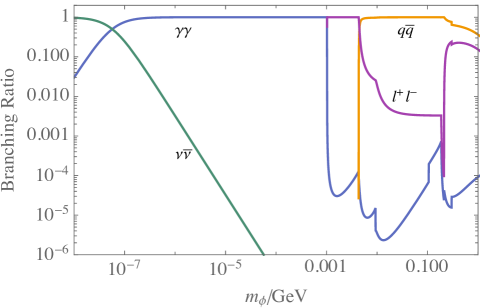
Figure 3: Branching ratios of the decay of the conformal dark matter.

III.4 Lyman-$\alpha$ constraints

Dark matter candidates with a non-negligible contribution to the cosmological background pressure can alter the matter power spectrum of density fluctuations by erasing overdensities on small physical scales. As a result this introduces a cutoff at large Fourier wavenumbers compared to the power spectrum expected within the $\Lambda$CDM cosmology. Absorption lines around $\sim 100\,$nm of light emitted by distant quasars at redshifts $z\sim 2-6$ by the neutral Hydrogen of the intergalactic medium, known as the Lyman-$\alpha$ forest, allow to probe the matter power spectrum on scales $k\sim(0.1-10)\,h\,\text{Mpc}^{-1}$. For a given dark matter phase space distribution, the Lyman-$\alpha$ forest can be used to set a bound on the DM mass or alternatively the equation-of-state parameter of such species. The Lyman-$\alpha$ bound is typically given in terms of a mass for Warm Dark Matter (WDM) Narayanan:2000tp ; Viel:2005qj ; Viel:2013fqw ; Baur:2015jsy ; Irsic:2017ixq ; Palanque-Delabrouille:2019iyz ; Garzilli:2019qki ,

$$m_{\rm WDM}\;\gtrsim\;m_{\rm WDM}^{\text{Ly}-\alpha}\;=\;(1.9-5.3)~{}\text{keV at 95\% C.L.}\,,$$ (46)

whose precise value depends on the specific analysis. As shown in Ref. Ballesteros:2020adh , DM particles produced in the early universe via scattering off SM particles inherit a phase space distribution different from the thermal distributions of their progenitors, which in our case can be well fitted by Ballesteros:2020adh

$$f(q)\,\propto\,q^{-0.29}\,e^{-1.1\,q}\,,$$ (47)

where $q$ is the DM comoving momentum defined as

$$q\equiv\dfrac{p\,a(t)}{T_{0}}\left(\frac{g_{*s}^{\rm RH}}{g_{*s}^{0}}\right)^{1/3}\,,$$ (48)

where $p$ is the DM momentum, $T_{0}$ the photon temperature at the present time, $g_{*s}^{0}$ and $g_{*s}^{\rm RH}$ are respectively the effective entropic degrees of freedom at present time and reheating. As the DM distribution is different from the WDM thermal distribution, the Lyman-$\alpha$ bound on the WDM mass cannot be used directly. However, it can be mapped into our scenario by using an equation-of-state matching procedure Ballesteros:2020adh , i.e. finding the value of $m_{\phi}$ such that

$$w(m_{\phi})=w_{\rm WDM}(m_{\rm WDM}^{\text{Ly}-\alpha})\,,$$ (49)

where $w\equiv\bar{P}/\bar{\rho}$ is the equation-of-state parameter defined as the ratio of the background DM pressure over background energy density which should be computed using our DM distribution of Eq. (47). From the condition of Eq. (49), the lower bound from the Lyman-$\alpha$ analysis can be translated into our scenario as

$$m_{\phi}\gtrsim 7.2~{}\text{keV}\,\left(\dfrac{m_{\rm WDM}^{{\rm Ly-}\alpha}}{3~{}\text{keV}}\right)^{4/3}\left(\dfrac{106.75}{g_{*s}^{\rm RH}}\right)^{1/3}\,.$$ (50)

Notice that taking the most or least conservative value of $m_{\rm WDM}^{{\rm Ly-}\alpha}$ in Eq. (46) represent respectively a stronger or weaker bound by a factor $\sim 2$.

IV IV. Analysis

We show in Fig. 4 the combined constraints from the dark matter lifetime and the relic abundance in the plane ($m_{\phi}$, $T_{\mathrm{RH}}$). The gamma-ray constraints on the lifetime of $\phi$ is extracted from different observations: XMM-Newton observations of M31 Boyarsky:2007ay for $m_{\phi}\lesssim 10$ keV, NuSTAR observation of the bullet cluster Riemer-Sorensen:2015kqa for $m_{\phi}\gtrsim 10$ keV and INTEGRAL Yuksel:2007dr for $m_{\phi}\gtrsim 100$ keV. We also show in Fig. 4 the Lyman-$\alpha$ limit obtained from Eq. (50) taking the more conservative bound $m_{\rm WDM}^{{\rm Ly-}\alpha}=1.9$ keV from Eq. (46), giving $m_{\phi}\gtrsim 3.9$ keV.

We illustrate as a potential smoking gun signature the point (star) corresponding to a dark matter mass $m_{\phi}=7.1$ keV and a lifetime $\tau_{\phi}\simeq 5\times 10^{27}$ seconds. These values correspond to the monochromatic X-ray observation made by the satellite XMM-Newton interpreted as a signal of dark matter decay Bulbul:2014sua . Notice that this benchmark point is actually in tension with the least conservative bound of Eq. (46).

The procedure to obtain this plot is straightforward. For each dark matter mass, we extracted the upper bound on $\alpha$ from Eq. (43) respecting the lifetime constraints. In turn, this upper bound on $\alpha$ gives a lower bound on $T_{\mathrm{RH}}$, needed to fulfill the relic abundance from Eq. (26). The points situated on the dashed/purple line satisfy thus the lifetime limits and $\Omega_{\phi}h^{2}\simeq 0.12$, whereas the ones below the line are excluded by X-ray constraints, and the one above the line are allowed given a much longer lifetime. In other words, if a monochromatic signal is observed in the range 1 keV-1 MeV, the mass being determined by the position of the peak, and the lifetime by the height of the peak, it would be possible to deduce the reheating temperature needed to respect the cosmological limit on dark matter abundance. Hence our model is extremely predictive. Notice also that we stopped our analysis at $m_{\phi}\simeq 0.1$ MeV, because the reheating temperature needed to fulfill the Planck constraints is above the inflaton mass, $m_{\Phi}=3\times 10^{13}$ GeV we considered in addition to the fact that if $m_{\phi}>2m_{e}\sim$ MeV, achieving the correct relic density is incompatible with the constraints on the dark matter lifetime.

Notice that our treatment hides the dependence on $\alpha$ of the parameter space, replacing it by $\tau_{\phi}$. However it can be interesting to evaluate the BSM scale $\Lambda=\frac{M_{P}}{\alpha}$ for some benchmark points. A point at the edge of the limit above the star in the Fig. 4 corresponds to the parameters

$$(m_{\phi},T_{\mathrm{RH}},\alpha)=(7.1~{}\rm{keV},3.5\times 10^{10}~{}\rm{GeV},7400)$$

$$~{}\leftrightarrow(\Omega h^{2},\tau_{\phi})=(0.12,8.7\times 10^{27}~{}s.).$$

We see that the corresponding BSM scale $\Lambda\simeq 3.2\times 10^{14}~{}\mathrm{GeV}~{}\gtrsim m_{\Phi}$, fully justifying our approach. Notice also that the more stringent the limit from X-ray observations, the smaller the upper bound on $\alpha$, and the more consistent our procedure, pushing the BSM scale toward the Planck scale.

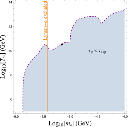
Figure 4: Parameter space allowed by the combined cosmological and X-ray constraints in the plane ($m_{\phi}$, $T_{\mathrm{RH}}$). The points situated on the dashed/purple line respect the lifetime limits and $\Omega h^{2}\simeq 0.1$, whereas the star indicates the monochromatic signal observed by XMM-Newton Bulbul:2014sua . The points on the left of the vertical line are excluded by the Lyman-$\alpha$ constraint (see the text for details).

V V. Conclusion

In this work, we show that a dark matter candidate $\phi$, conformally coupled to the Standard Model allows for a sufficient production even for Planck-reduced coupling. The high temperatures generated by the inflaton decay in the earliest stage of reheating are sufficient to overcome the feeble coupling whereas in the meantime, for dark matter masses below $\lesssim 1$ MeV, the lifetime is sufficiently large to respect the X-ray and $\gamma-$ray constraints of a variety of telescope experiments. We also included the limits on $m_{\phi}$ from the more recent Lyman-$\alpha$ analysis, $m_{\phi}\gtrsim 3.9$ keV. Our construction is very predictive as summarized by Eq. (45) and Fig. 4 where we exhibit the parameter space allowed and observable by the future experimental analysis of the X-ray sky. In particular, triangle loops of decoupled fermions generate decay processes of the type $\phi\rightarrow\gamma\gamma$ whose typical signature (a monochromatic photon) is a smoking gun signal for dark matter searches. Such an observation, combined with the relic abundance constraint would determine completely the parameter space of our model. In addition to the indirect searches, new techniques of the direct detection searches for dark matter may allow us to explore the parameter space down to keV mass scales in the future Alexander:2016aln .

Acknowledgments: The authors want to thank especially Keith Olive, Emilian Dudas, Marcos Garcia, Pyungwon Ko and Dr. Biglouche for very insightful discussions. This project has received support from the European Union’s Horizon 2020 research and innovation programme under the Marie Skodowska -Curie grant agreement No 860881-HIDDeN and the CNRS PICS MicroDark.. The work of MP was supported by the Spanish Agencia Estatal de Investigación through the grants FPA2015-65929-P (MINECO/FEDER, UE), PGC2018-095161-B-I00, IFT Centro de Excelencia Severo Ochoa SEV-2016-0597, and Red Consolider MultiDark FPA2017-90566-REDC. The work of KK was supported in part by a KIAS Individual Grant (Grant No. PG080301) at Korea Institute for Advanced Study.

Appendix

Appendix A A. Derivation of the Lagrangian

To make our framework clearer, we summarize here the relevant part of the Lagrangian. The dark matter sector is constructed by introducing the conformal factor as $\tilde{g}_{\mu\nu}=C(\phi)g_{\mu\nu}$, where we work on the mostly-minus convention, $(+,-,-,-)$, for the metric. To reproduce the Einstein-Hilbert action in the $g_{\mu\nu}$-frame, we define the gravity sector in the $\tilde{g}_{\mu\nu}$-frame by

$${\cal S}_{\rm grav}=\frac{M_{P}^{2}}{2}\int\mathop{}\!\mathrm{d}^{4}x\sqrt{-\tilde{g}}C^{-1}\tilde{R},$$ (51)

where $\tilde{R}$ is the Ricci scalar in the $\tilde{g}_{\mu\nu}$-frame. Thus, from the relation

$$C\tilde{R}\,=\,R+\frac{(d-1)(d-2)}{4}g^{\mu\nu}(\partial_{\mu}\ln C)(\partial_{\nu}\ln C)\\ +(d-1)\partial^{2}\ln C\,,$$ (52)

for $d$-dimensional space-times (and we will take $d=4$), we obtain

$${\cal S}_{\rm grav}=\frac{M_{P}^{2}}{2}\int\mathop{}\!\mathrm{d}^{4}x\sqrt{-g}\left[R+\frac{3}{2}g^{\mu\nu}(\partial_{\mu}\ln C)(\partial_{\nu}\ln C)\right].$$ (53)

By defining the dark matter sector as

$${\cal S}_{\rm DM}=\int\mathop{}\!\mathrm{d}^{4}x\sqrt{-\tilde{g}}\left[M_{P}^{2}K\tilde{g}^{\mu\nu}(\partial_{\mu}C^{1/2})(\partial_{\nu}C^{1/2})-\tilde{V}\right],$$ (54)

with $K$ and $\tilde{V}$ being an arbitrary constant and the scalar potential in the $\tilde{g}_{\mu\nu}$-frame, respectively, we end up with

$${\cal S}_{\rm grav}+{\cal S}_{\rm DM}=\int\mathop{}\!\mathrm{d}^{4}x\sqrt{-g}\Big{[}\frac{M_{P}^{2}}{2}R+\frac{1}{2}g^{\mu\nu}(\partial_{\mu}\phi)(\partial_{\nu}\phi)\\ -\frac{1}{2}m_{\phi}^{2}\phi^{2}\Big{]},$$ (55)

where we have used $C(\phi)=e^{\alpha\phi/M_{P}}$, and $\tilde{V}/C^{2}\equiv(1/2)m_{\phi}^{2}\phi^{2}$. We also assume $K=2/\alpha^{2}-3$, so that the kinetic term for $\phi$ takes the canonical form in the $g_{\mu\nu}$-frame. The action of the Standard Model sector is

$${\cal S}_{\rm SM}=\int\mathop{}\!\mathrm{d}^{4}x\sqrt{-\tilde{g}}\tilde{\cal L}_{\rm SM}\,,$$ (56)

where the metric in $\tilde{\cal L}_{\rm SM}$ is assumed to be $\tilde{g}_{\mu\nu}$. To see the interaction between $\phi$ and the Standard Model particles, it is convenient to expand $\tilde{g}_{\mu\nu}$ as $\tilde{g}_{\mu\nu}\simeq g_{\mu\nu}+\delta g_{\mu\nu}$ with $\delta g_{\mu\nu}=(\alpha\phi/M_{P})g_{\mu\nu}$. Thus, we obtain

$${\cal S}_{\rm SM}\simeq\int\mathop{}\!\mathrm{d}^{4}x\sqrt{-g}{\cal L}_{\rm SM}+\delta{\cal S}_{\rm SM},$$ (57)

with

$$\delta{\cal S}_{\rm SM}=-\frac{\alpha}{2}\frac{\phi}{M_{P}}\int\mathop{}\!\mathrm{d}^{4}x\sqrt{-g}g^{\mu\nu}T^{\rm SM}_{\mu\nu}\,,$$ (58)

where the SM energy-momentum tensor $T^{\rm SM}_{\mu\nu}$ is defined as

$$T^{\rm SM}_{\mu\nu}\equiv\dfrac{2}{\sqrt{-g}}\dfrac{\delta(\sqrt{-g}\mathcal{L}_{\text{SM}})}{\delta g^{\mu\nu}}\,,$$ (59)

which is explicitly written in Eqs. (12-16).

Appendix B B. A possible coupling to the inflaton

Assuming that the DM scalar field $\phi$ interacts with the inflaton field $\Phi$ via a renormalizable coupling (in the Einstein frame) like

$$\mathcal{V}\,=\,\kappa\phi^{2}\Phi^{2}\,,$$ (60)

which generates an effective mass for the DM during inflation

$$m_{\phi,\rm eff}^{2}\,=\,\dfrac{\partial^{2}\mathcal{V}}{\partial\phi^{2}}\sim\kappa M_{P}^{2}\,.$$ (61)

A contribution to the DM density is generated at the end of inflation by $4$-point processes corresponding to the time dependent dissipation rate GKMO2

$$\Gamma_{\Phi\Phi\rightarrow\phi\phi}\,=\,\dfrac{\kappa^{2}\rho_{\Phi}(t)}{8\pi m_{\Phi}^{3}}\,\,$$ (62)

which corresponds to the following contribution to the relic density

$$\frac{\Omega_{\phi}h^{2}}{0.1}\simeq \left(\dfrac{m_{\phi}}{10\,\rm{keV}}\right)\left(\dfrac{\kappa}{2.4\times 10^{-4}}\right)^{2}\left(\dfrac{y}{10^{-5}}\right)\left(\dfrac{g_{s}^{\rm inf}}{106.75}\right)^{3/4}$$

$$\times\left(\dfrac{m_{\Phi}}{3\times 10^{13}\,\rm{GeV}}\right)^{-7/2}\left(\dfrac{\rho^{\rm end}_{\Phi}}{0.175\,m_{\Phi}^{2}M_{P}^{2}}\right)^{1/2}$$ (63)

where $y\equiv(8\pi\Gamma_{\Phi}/m_{\Phi})^{1/2}$ is the typical dimensionless coupling of the inflaton to the SM inducing reheating. $\rho^{\rm end}_{\Phi}$ is the energy stored in the inflaton field at the end of inflation.

Isocurvature perturbations can be induced if the DM effective mass becomes lower than the Hubble expansion rate during inflation. According to Eq. (61), this could occur only for very small values of $\kappa$. However for such small values of $\kappa$, the DM production induced by such coupling according to Eq. (63) would be negligible and therefore we expect both the DM background density and fluctuations to be both predominantly produced by the freeze-in mechanism. In this case, the DM fluctuations would be inherited from the SM plasma and therefore are expected to be adiabatic. A more quantitative analysis of the previous statement goes beyond this work.

References

- (1) F. Zwicky, “Die Rotverschiebung von extragalaktischen Nebeln,” Helv. Phys. Acta 6 (1933), 110-127 doi:10.1007/s10714-008-0707-4
- (2) H. W. Babcock, "The rotation of the Andromeda Nebula". Lick Observatory Bulletin N. 498.
- (3) J. Ostriker and P. Peebles, Astrophys. J. 186 (1973), 467-480 doi:10.1086/152513
- (4) J. Gunn, B. Lee, I. Lerche, D. Schramm and G. Steigman, Astrophys. J. 223 (1978), 1015-1031 doi:10.1086/156335
- (5) P. A. R. Ade et al. [Planck Collaboration], Astron. Astrophys. 594, A13 (2016) [arXiv:1502.01589 [astro-ph.CO]]; N. Aghanim et al. [Planck Collaboration], arXiv:1807.06209 [astro-ph.CO].
- (6) H. Pagels and J. R. Primack, Phys. Rev. Lett. 48, 223 (1982);
- (7) D. V. Nanopoulos, K. A. Olive and M. Srednicki, Phys. Lett. B 127, 30 (1983); M. Y. Khlopov and A. D. Linde, Phys. Lett. B 138, 265 (1984); K. A. Olive, D. N. Schramm and M. Srednicki, Nucl. Phys. B 255, 495 (1985);
- (8) G. Arcadi, M. Dutra, P. Ghosh, M. Lindner, Y. Mambrini, M. Pierre, S. Profumo and F. S. Queiroz, Eur. Phys. J. C 78 (2018) no.3, 203 [arXiv:1703.07364 [hep-ph]].
- (9) J. A. Casas, D. G. Cerdeño, J. M. Moreno and J. Quilis, JHEP 1705 (2017) 036 [arXiv:1701.08134 [hep-ph]]. A. Djouadi, O. Lebedev, Y. Mambrini and J. Quevillon, Phys. Lett. B 709 (2012) 65 [arXiv:1112.3299 [hep-ph]]; A. Djouadi, A. Falkowski, Y. Mambrini and J. Quevillon, Eur. Phys. J. C 73 (2013) no.6, 2455 [arXiv:1205.3169 [hep-ph]]; O. Lebedev, H. M. Lee and Y. Mambrini, Phys. Lett. B 707 (2012) 570 [arXiv:1111.4482 [hep-ph]]; Y. Mambrini, Phys. Rev. D 84 (2011) 115017 [arXiv:1108.0671 [hep-ph]].
- (10) J. Ellis, A. Fowlie, L. Marzola and M. Raidal, Phys. Rev. D 97, no.11, 115014 (2018) [arXiv:1711.09912 [hep-ph]]; G. Arcadi, Y. Mambrini and F. Richard, JCAP 1503 (2015) 018 [arXiv:1411.2985 [hep-ph]]; J. Kearney, N. Orlofsky and A. Pierce, Phys. Rev. D 95, no.3, 035020 (2017) [arXiv:1611.05048 [hep-ph]]; M. Escudero, A. Berlin, D. Hooper and M. X. Lin, JCAP 1612 (2016) 029 [arXiv:1609.09079 [hep-ph]].
- (11) A. Alves, S. Profumo and F. S. Queiroz, JHEP 1404 (2014) 063 [arXiv:1312.5281 [hep-ph]]. O. Lebedev and Y. Mambrini, Phys. Lett. B 734 (2014) 350 [arXiv:1403.4837 [hep-ph]]; G. Arcadi, Y. Mambrini, M. H. G. Tytgat and B. Zaldivar, JHEP 1403 (2014) 134 [arXiv:1401.0221 [hep-ph]]; O. Lebedev and Y. Mambrini, Phys. Lett. B 734 (2014) 350 [arXiv:1403.4837 [hep-ph]].
- (12) E. Aprile et al. [XENON Collaboration], Phys. Rev. Lett. 121 (2018) no.11, 111302 [arXiv:1805.12562 [astro-ph.CO]].
- (13) D. S. Akerib et al. [LUX Collaboration], Phys. Rev. Lett. 118 (2017) no.2, 021303 [arXiv:1608.07648 [astro-ph.CO]].
- (14) X. Cui et al. [PandaX-II Collaboration], Phys. Rev. Lett. 119 (2017) no.18, 181302 [arXiv:1708.06917 [astro-ph.CO]].
- (15) L. J. Hall, K. Jedamzik, J. March-Russell and S. M. West, JHEP 1003 (2010) 080 [arXiv:0911.1120 [hep-ph]]; X. Chu, T. Hambye and M. H. G. Tytgat, JCAP 1205 (2012) 034 [arXiv:1112.0493 [hep-ph]]; A. Biswas, D. Borah and A. Dasgupta, Phys. Rev. D 99, no.1, 015033 (2019) [arXiv:1805.06903 [hep-ph]]; B. Barman, D. Borah and R. Roshan, JCAP 11 (2020), 021 doi:10.1088/1475-7516/2020/11/021 [arXiv:2007.08768 [hep-ph]].
- (16) K. Benakli, Y. Chen, E. Dudas and Y. Mambrini, Phys. Rev. D 95, no. 9, 095002 (2017) doi:10.1103/PhysRevD.95.095002 [arXiv:1701.06574 [hep-ph]]; E. Dudas, Y. Mambrini and K. Olive, Phys. Rev. Lett. 119 (2017) no.5, 051801 [arXiv:1704.03008 [hep-ph]]; E. Dudas, T. Gherghetta, Y. Mambrini and K. A. Olive, Phys. Rev. D 96 (2017) no.11, 115032 [arXiv:1710.07341 [hep-ph]]; E. Dudas, T. Gherghetta, K. Kaneta, Y. Mambrini and K. A. Olive, Phys. Rev. D 98, no. 1, 015030 (2018) [arXiv:1805.07342 [hep-ph]]. S. A. R. Ellis, T. Gherghetta, K. Kaneta and K. A. Olive, Phys. Rev. D 98, no. 5, 055009 (2018) [arXiv:1807.06488 [hep-ph]].
- (17) Y. Mambrini, K. A. Olive, J. Quevillon and B. Zaldivar, Phys. Rev. Lett. 110 (2013) no.24, 241306 [arXiv:1302.4438 [hep-ph]]; N. Nagata, K. A. Olive and J. Zheng, JHEP 1510, 193 (2015) [arXiv:1509.00809 [hep-ph]]; Y. Mambrini, N. Nagata, K. A. Olive and J. Zheng, Phys. Rev. D 93 (2016) no.11, 111703 [arXiv:1602.05583 [hep-ph]]; X. Chu, Y. Mambrini, J. Quevillon and B. Zaldivar, JCAP 1401 (2014) 034 [arXiv:1306.4677 [hep-ph]]; Y. Mambrini, N. Nagata, K. A. Olive, J. Quevillon and J. Zheng, Phys. Rev. D 91 (2015) no.9, 095010 [arXiv:1502.06929 [hep-ph]]; N. Nagata, K. A. Olive and J. Zheng, JCAP 1702, no. 02, 016 (2017) [arXiv:1611.04693 [hep-ph]].
- (18) G. Bhattacharyya, M. Dutra, Y. Mambrini and M. Pierre, Phys. Rev. D 98 (2018) no.3, 035038 [arXiv:1806.00016 [hep-ph]]; A. Banerjee, G. Bhattacharyya, D. Chowdhury and Y. Mambrini, JCAP 12 (2019), 009 doi:10.1088/1475-7516/2019/12/009 [arXiv:1905.11407 [hep-ph]]; K. Kaneta, Z. Kang and H. S. Lee, JHEP 02, 031 (2017) doi:10.1007/JHEP02(2017)031 [arXiv:1606.09317 [hep-ph]]; B. Barman, S. Bhattacharya and B. Grzadkowski, JHEP 12 (2020), 162 doi:10.1007/JHEP12(2020)162 [arXiv:2009.07438 [hep-ph]].
- (19) N. Bernal, M. Dutra, Y. Mambrini, K. Olive, M. Peloso and M. Pierre, Phys. Rev. D 97 (2018) no.11, 115020 [arXiv:1803.01866 [hep-ph]]; Y. J. Kang and H. M. Lee, [arXiv:2003.09290 [hep-ph]].
- (20) N. Bernal, A. Donini, M. G. Folgado and N. Rius, JHEP 09 (2020), 142 doi:10.1007/JHEP09(2020)142 [arXiv:2004.14403 [hep-ph]].
- (21) L. Heurtier and F. Huang, Phys. Rev. D 100 (2019) no.4, 043507 [arXiv:1905.05191 [hep-ph]]; A. Berlin, D. Hooper and G. Krnjaic, Phys. Rev. D 94 (2016) no.9, 095019 [arXiv:1609.02555 [hep-ph]]; A. Berlin, D. Hooper and G. Krnjaic, Phys. Lett. B 760 (2016) 106 [arXiv:1602.08490 [hep-ph]]; M. Heikinheimo, T. Tenkanen, K. Tuominen and V. Vaskonen, Phys. Rev. D 94 (2016) no.6, 063506 Erratum: [Phys. Rev. D 96 (2017) no.10, 109902] doi:10.1103/PhysRevD.96.109902, 10.1103/PhysRevD.94.063506 [arXiv:1604.02401 [astro-ph.CO]]; K. Kaneta, H. S. Lee and S. Yun, Phys. Rev. Lett. 118, no.10, 101802 (2017) doi:10.1103/PhysRevLett.118.101802 [arXiv:1611.01466 [hep-ph]]; L. Heurtier and H. Partouche, Phys. Rev. D 101 (2020) no.4, 043527 doi:10.1103/PhysRevD.101.043527 [arXiv:1912.02828 [hep-ph]].
- (22) Y. Ema, R. Jinno, K. Mukaida and K. Nakayama, JCAP 05 (2015), 038 doi:10.1088/1475-7516/2015/05/038 [arXiv:1502.02475 [hep-ph]]; Y. Ema, R. Jinno, K. Mukaida and K. Nakayama, Phys. Rev. D 94 (2016) no.6, 063517 doi:10.1103/PhysRevD.94.063517 [arXiv:1604.08898 [hep-ph]]; Y. Ema, K. Nakayama and Y. Tang, JHEP 09 (2018), 135 doi:10.1007/JHEP09(2018)135 [arXiv:1804.07471 [hep-ph]]; Y. Mambrini and K. A. Olive, [arXiv:2102.06214 [hep-ph]]; N. Bernal, A. Donini, M. G. Folgado and N. Rius, [arXiv:2012.10453 [hep-ph]]; S. Hashiba and J. Yokoyama, Phys. Rev. D 99 (2019) no.4, 043008 doi:10.1103/PhysRevD.99.043008 [arXiv:1812.10032 [hep-ph]]; A. Ahmed, B. Grzadkowski and A. Socha, JHEP 08 (2020), 059 doi:10.1007/JHEP08(2020)059 [arXiv:2005.01766 [hep-ph]]; M. Chianese, B. Fu and S. F. King, JCAP 01 (2021), 034 doi:10.1088/1475-7516/2021/01/034 [arXiv:2009.01847 [hep-ph]]; Y. J. Kang and H. M. Lee, Eur. Phys. J. C 80 (2020) no.7, 602 doi:10.1140/epjc/s10052-020-8153-x [arXiv:2001.04868 [hep-ph]].
- (23) P. Anastasopoulos, K. Kaneta, Y. Mambrini and M. Pierre, Phys. Rev. D 102 (2020) no.5, 055019 doi:10.1103/PhysRevD.102.055019 [arXiv:2007.06534 [hep-ph]]; P. Anastasopoulos, P. Betzios, M. Bianchi, D. Consoli and E. Kiritsis, JHEP 19 (2020), 113 doi:10.1007/JHEP10(2019)113 [arXiv:1811.05940 [hep-ph]]; P. Anastasopoulos, M. Bianchi, D. Consoli and E. Kiritsis, [arXiv:2010.07320 [hep-ph]].
- (24) D. Chowdhury, E. Dudas, M. Dutra and Y. Mambrini, Phys. Rev. D 99 (2019) no.9, 095028 [arXiv:1811.01947 [hep-ph]].
- (25) N. Bernal, M. Heikinheimo, T. Tenkanen, K. Tuominen and V. Vaskonen, Int. J. Mod. Phys. A 32 (2017) no.27, 1730023 [arXiv:1706.07442 [hep-ph]].
- (26) D. V. Volkov and V. P. Akulov, Phys. Lett. B 46 (1973) 109; E. A. Ivanov and A. A. Kapustnikov, J. Phys. A 11 (1978) 2375.
- (27) G. Nordstrom, Ann. Phys. 42 533 (1913).
- (28) C. Brans and R.H. Dicke, Phys. Rev. D15, 1458 (1977); R.H. Dicke, Phys. Rev. 125, 2163 (1962).
- (29) P.A.M dirac, Proc. Roy. Soc. London A333, 403 (1973)
- (30) J. D. Bekenstein, Phys. Rev. D 48 (1993), 3641-3647 doi:10.1103/PhysRevD.48.3641 [arXiv:gr-qc/9211017 [gr-qc]].
- (31) J. D. Bekenstein, in “The Sixth Marcel Grossmann Meeting on General Relativity,” ed. H. Sato (World Publishing, Singapore, 1992).
- (32) S. M. Choi, Y. J. Kang, H. M. Lee and K. Yamashita, JHEP 05, 060 (2019) doi:10.1007/JHEP05(2019)060 [arXiv:1902.03781 [hep-ph]].
- (33) E. Dudas, L. Heurtier, Y. Mambrini, K. A. Olive and M. Pierre, Phys. Rev. D 101 (2020) no.11, 115029 doi:10.1103/PhysRevD.101.115029 [arXiv:2003.02846 [hep-ph]].
- (34) M. A. G. Garcia, K. Kaneta, Y. Mambrini and K. A. Olive, Phys. Rev. D 101 (2020) no.12, 123507 [arXiv:2004.08404 [hep-ph]].
- (35) M. A. G. Garcia, K. Kaneta, Y. Mambrini and K. A. Olive, [arXiv:2012.10756 [hep-ph]];
- (36) K. Kaneta, Y. Mambrini and K. A. Olive, Phys. Rev. D 99 (2019) no.6, 063508 doi:10.1103/PhysRevD.99.063508 [arXiv:1901.04449 [hep-ph]].
- (37) T. Moroi and W. Yin, [arXiv:2011.09475 [hep-ph]].
- (38) B. Bellazzini, C. Csaki, J. Hubisz, J. Serra and J. Terning, Eur. Phys. J. C 73 (2013) no.2, 2333 doi:10.1140/epjc/s10052-013-2333-x [arXiv:1209.3299 [hep-ph]].
- (39) A. Dusoye, A. de la Cruz-Dombriz, P. Dunsby and N. J. Nunes, [arXiv:2006.16962 [gr-qc]]; C. van de Bruck, J. Mifsud, J. P. Mimoso and N. J. Nunes, JCAP 11 (2016), 031 doi:10.1088/1475-7516/2016/11/031 [arXiv:1605.03834 [gr-qc]].
- (40) P. Brax and P. Valageas, Phys. Rev. D 95 (2017) no.4, 043515 doi:10.1103/PhysRevD.95.043515 [arXiv:1611.08279 [astro-ph.CO]].
- (41) S. Trojanowski, P. Brax and C. van de Bruck, Phys. Rev. D 102 (2020) no.2, 023035 doi:10.1103/PhysRevD.102.023035 [arXiv:2006.01149 [hep-ph]]. S. Trojanowski, P. Brax and C. van de Bruck, Phys. Rev. D 102 (2020) no.2, 023035 doi:10.1103/PhysRevD.102.023035 [arXiv:2006.01149 [hep-ph]]; J. A. R. Cembranos and A. L. Maroto, Int. J. Mod. Phys. 31 (2016) no.14n15, 1630015 doi:10.1142/S0217751X16300155 [arXiv:1602.07270 [hep-ph]].
- (42) P. Brax, K. Kaneta, Y. Mambrini and M. Pierre, Phys. Rev. D 103, no.1, 015028 (2021) doi:10.1103/PhysRevD.103.015028 [arXiv:2011.11647 [hep-ph]].
- (43) J. Sakstein, Phys. Rev. D 91 (2015) no.2, 024036 doi:10.1103/PhysRevD.91.024036 [arXiv:1409.7296 [astro-ph.CO]]; J. Sakstein, JCAP 12 (2014), 012 doi:10.1088/1475-7516/2014/12/012 [arXiv:1409.1734 [astro-ph.CO]].
- (44) M. A. G. Garcia, Y. Mambrini, K. A. Olive and M. Peloso, Phys. Rev. D 96, no.10, 103510 (2017) doi:10.1103/PhysRevD.96.103510 [arXiv:1709.01549 [hep-ph]].
- (45) B. Barman, D. Borah and R. Roshan, [arXiv:2103.01675 [hep-ph]].
- (46) M. A. G. Garcia and M. A. Amin, Phys. Rev. D 98, no. 10, 103504 (2018) [arXiv:1806.01865 [hep-ph]]; K. Harigaya, K. Mukaida and M. Yamada, JHEP 07 (2019), 059 doi:10.1007/JHEP07(2019)059 [arXiv:1901.11027 [hep-ph]]; K. Harigaya, M. Kawasaki, K. Mukaida and M. Yamada, Phys. Rev. D 89 (2014) no.8, 083532 [arXiv:1402.2846 [hep-ph]].
- (47) F. Elahi, C. Kolda and J. Unwin, JHEP 03 (2015), 048 doi:10.1007/JHEP03(2015)048 [arXiv:1410.6157 [hep-ph]]; N. Bernal, J. Rubio and H. Veermäe, [arXiv:2004.13706 [hep-ph]]; N. Bernal, F. Elahi, C. Maldonado and J. Unwin, JCAP 11 (2019), 026 doi:10.1088/1475-7516/2019/11/026 [arXiv:1909.07992 [hep-ph]]; A. Di Marco, G. De Gasperis, G. Pradisi and P. Cabella, Phys. Rev. D 100 (2019) no.12, 123532 doi:10.1103/PhysRevD.100.123532 [arXiv:1907.06084 [astro-ph.CO]]; A. Di Marco, G. Pradisi and P. Cabella, Phys. Rev. D 98 (2018) no.12, 123511 doi:10.1103/PhysRevD.98.123511 [arXiv:1807.05916 [astro-ph.CO]]; A. Di Marco and G. Pradisi, [arXiv:2102.00326 [gr-qc]].
- (48) Y. Mambrini, S. Profumo and F. S. Queiroz, Phys. Lett. B 760 (2016), 807-815 doi:10.1016/j.physletb.2016.07.076 [arXiv:1508.06635 [hep-ph]].
- (49) V. K. Narayanan, D. N. Spergel, R. Dave and C. P. Ma, Astrophys. J. Lett. 543 (2000), L103-L106 doi:10.1086/317269 [arXiv:astro-ph/0005095 [astro-ph]].
- (50) M. Viel, J. Lesgourgues, M. G. Haehnelt, S. Matarrese and A. Riotto, Phys. Rev. D 71 (2005), 063534 doi:10.1103/PhysRevD.71.063534 [arXiv:astro-ph/0501562 [astro-ph]].
- (51) M. Viel, G. D. Becker, J. S. Bolton and M. G. Haehnelt, Phys. Rev. D 88 (2013), 043502 doi:10.1103/PhysRevD.88.043502 [arXiv:1306.2314 [astro-ph.CO]].
- (52) J. Baur, N. Palanque-Delabrouille, C. Yèche, C. Magneville and M. Viel, JCAP 08 (2016), 012 doi:10.1088/1475-7516/2016/08/012 [arXiv:1512.01981 [astro-ph.CO]].
- (53) V. Iršič, M. Viel, M. G. Haehnelt, J. S. Bolton, S. Cristiani, G. Cupani, T. S. Kim, V. D’Odorico, S. López and S. Ellison, et al. Phys. Rev. D 96 (2017) no.2, 023522 doi:10.1103/PhysRevD.96.023522 [arXiv:1702.01764 [astro-ph.CO]].
- (54) N. Palanque-Delabrouille, C. Yèche, N. Schöneberg, J. Lesgourgues, M. Walther, S. Chabanier and E. Armengaud, JCAP 04 (2020), 038 doi:10.1088/1475-7516/2020/04/038 [arXiv:1911.09073 [astro-ph.CO]].
- (55) A. Garzilli, O. Ruchayskiy, A. Magalich and A. Boyarsky, [arXiv:1912.09397 [astro-ph.CO]].
- (56) G. Ballesteros, M. A. G. Garcia and M. Pierre, [arXiv:2011.13458 [hep-ph]].
- (57) A. Boyarsky, D. Iakubovskyi, O. Ruchayskiy and V. Savchenko, Mon. Not. Roy. Astron. Soc. 387 (2008), 1361 [arXiv:0709.2301 [astro-ph]].
- (58) S. Riemer-Sørensen, D. Wik, G. Madejski, S. Molendi, F. Gastaldello, F. A. Harrison, W. W. Craig, C. J. Hailey, S. E. Boggs and F. E. Christensen, et al. Astrophys. J. 810 (2015) no.1, 48 doi:10.1088/0004-637X/810/1/48 [arXiv:1507.01378 [astro-ph.CO]].
- (59) H. Yuksel and M. D. Kistler, Phys. Rev. D 78 (2008), 023502 [arXiv:0711.2906 [astro-ph]].
- (60) V. De Romeri, D. Karamitros, O. Lebedev and T. Toma, JHEP 10 (2020), 137 doi:10.1007/JHEP10(2020)137 [arXiv:2003.12606 [hep-ph]].
- (61) M. A. G. Garcia, Y. Mambrini, K. A. Olive and S. Verner, Phys. Rev. D 102 (2020) no.8, 083533 doi:10.1103/PhysRevD.102.083533 [arXiv:2006.03325 [hep-ph]]; A. Falkowski, G. Isabella and C. S. Machado, [arXiv:2011.05339 [hep-ph]]; J. C. Criado, N. Koivunen, M. Raidal and H. Veermäe, Phys. Rev. D 102 (2020) no.12, 125031 doi:10.1103/PhysRevD.102.125031 [arXiv:2010.02224 [hep-ph]].
- (62) E. Dudas, Y. Mambrini and K. A. Olive, Phys. Rev. D 91 (2015), 075001 [arXiv:1412.3459 [hep-ph]]; E. Dudas, L. Heurtier, Y. Mambrini, K. A. Olive and M. Pierre, [arXiv:2003.02846 [hep-ph]]; L. Heurtier, Y. Mambrini and M. Pierre, Phys. Rev. D 99 (2019) no.9, 095014 doi:10.1103/PhysRevD.99.095014 [arXiv:1902.04584 [hep-ph]].
- (63) X. Chu, T. Hambye, T. Scarna and M. H. G. Tytgat, Phys. Rev. D 86 (2012), 083521 doi:10.1103/PhysRevD.86.083521 [arXiv:1206.2279 [hep-ph]].
- (64) E. Bulbul, M. Markevitch, A. Foster, R. K. Smith, M. Loewenstein and S. W. Randall, Astrophys. J. 789 (2014), 13 doi:10.1088/0004-637X/789/1/13 [arXiv:1402.2301 [astro-ph.CO]].
- (65) J. Alexander, M. Battaglieri, B. Echenard, R. Essig, M. Graham, E. Izaguirre, J. Jaros, G. Krnjaic, J. Mardon and D. Morrissey, et al. [arXiv:1608.08632 [hep-ph]].