Thermal Emission and Radioactive Lines, but No Pulsar, in the Broadband X-Ray Spectrum of Supernova 1987A

Abstract

Supernova 1987A offers a unique opportunity to study an evolving supernova in unprecedented detail over several decades. The X-ray emission is dominated by interactions between the ejecta and the circumstellar medium, primarily the equatorial ring (ER). We analyze 3.3 Ms of NuSTAR data obtained between 2012 and 2020, and two decades of XMM-Newton data. Since ${\sim}$2013, the flux below 2 keV has declined, the 3–8 keV flux has increased, but has started to flatten, and the emission above 10 keV has remained nearly constant. The spectra are well described by a model with three thermal shock components. Two components at 0.3 and 0.9 keV are associated with dense clumps in the ER, and a 4 keV component may be a combination of emission from diffuse gas in the ER and the surrounding low-density H ii region. We disfavor models that involve non-thermal X-ray emission and place constraints on non-thermal components, but cannot firmly exclude an underlying power law. Radioactive lines show a ⁴⁴Ti redshift of $670^{+520}_{-380}$ km s^-1, ⁴⁴Ti mass of $1.73_{-0.29}^{+0.27}\times{}10^{-4}$ M_☉, and ⁵⁵Fe mass of $<4.2\times{}10^{-4}$ M_☉. The 35–65 keV luminosity limit on the compact object is $2\times{}10^{34}$ erg s^-1, and $<15$ % of the 10–20 keV flux is pulsed. Considering previous limits, we conclude that there are currently no indications of a compact object, aside from a possible hint of dust heated by a neutron star in recent ALMA images.

1 Introduction

Supernova (SN) 1987A is the closest observed SN in more than four centuries (Arnett et al., 1989; McCray, 1993; McCray & Fransson, 2016). It is a core-collapse SN located in the Large Magellanic Cloud (LMC) and was first detected on 1987 February 23. The progenitor star, Sanduleak -69^∘ 202 (Sanduleak, 1970), was identified as a B3 Ia blue supergiant (West et al., 1987). The progenitor shaped the circumstellar medium (CSM) around SN 1987A and produced a triple-ring structure (Wampler et al., 1990; Burrows et al., 1995). This structure consists of two larger outer rings and a smaller equatorial ring (ER). Different explanations for this based on interacting winds (Blondin & Lundqvist, 1993; Martin & Arnett, 1995), binary mergers (Morris & Podsiadlowski, 2007; Menon & Heger, 2017; Utrobin et al., 2021), or rapid rotation (Chita et al., 2008) have been proposed. The three rings are nearly coaxial, forming an hourglass-like shape (Chevalier & Dwarkadas, 1995; Larsson et al., 2019). They are nearly circular, but appear elliptical because they are viewed at an inclination of ${\sim}$38–45° (Crotts & Heathcote, 2000; Tziamtzis et al., 2011). The X-ray emission that we study in this paper is primarily due to the interaction with this complex CSM.

At early times, the ejecta from SN 1987A propagated through a low-density H ii region inside of the ER, which gave rise to faint radio and X-ray emission (Staveley-Smith et al., 1992; Chevalier & Dwarkadas, 1995; Hasinger et al., 1996). After approximately 3000 d, the ejecta started interacting with the denser ER. This interaction produced a significant brightening in all wavebands (Bouchet et al., 2006; Park et al., 2006; Gröningsson et al., 2008; Ng et al., 2008; Dwek et al., 2010). Notably, high-density clumps inside the ER produced bright optical “hotspots” (Sonneborn et al., 1998; Lawrence et al., 2000). More recent observations show that the optical emission is declining and that new hotspots have appeared outside of the ER (Fransson et al., 2015; Larsson et al., 2019). Furthermore, the infrared (IR) emission has been declining since ${\sim}$9000 d (Arendt et al., 2016, 2020), X-rays below 2 keV started decreasing at 10,000 d (Frank et al., 2016; Ravi, 2019), and the radio blast wave is now reaccelerating (Cendes et al., 2018). These observations all show that most of the blast wave is now propagating past the ER, while the ER is being dissolved.

In addition to the long monitoring of SN 1987A in radio, optical, and X-rays, a potential GeV detection has recently been reported using Fermi data (Malyshev et al., 2019; Petruk et al., 2019). A major uncertainty is if the emission is truly originating from SN 1987A because the angular resolution of Fermi is insufficient to resolve SN 1987A from other nearby sources. If associated with SN 1987A, the data suggest an increase in the GeV flux by a factor of ${\sim}$2 between 2010 and 2018, which could indicate efficient cosmic ray acceleration in the shocks (Dwarkadas, 2013; Berezhko et al., 2015).

The X-ray emission produced by the interactions with the ER has been extensively studied in the literature (Burrows et al., 2000; Michael et al., 2002; Park et al., 2002, 2004, 2005, 2006, 2011; Zhekov et al., 2005, 2006, 2009, 2010; Haberl et al., 2006; Dewey et al., 2008, 2012; Heng et al., 2008; Racusin et al., 2009; Sturm et al., 2009, 2010; Maggi et al., 2012; Helder et al., 2013; Orlando et al., 2015, 2019; Frank et al., 2016; Miceli et al., 2019; Bray et al., 2020; Greco et al., 2021; Sun et al., 2021). For brevity, we only summarize the most relevant findings from the previous studies. The ER is resolved by Chandra, which allows for studies of the morphology and expansion velocity. Comparisons with other wavelengths show that X-rays below 2 keV are generally more strongly correlated with optical, whereas harder X-rays better follow the radio evolution. The X-ray emission has been interpreted as predominantly or completely of thermal origin. The detection of the Fe K line complex clearly shows that thermal emission is important at energies up to ${\sim}$10 keV.

Thermal models for the X-ray spectra require multiple components of different temperatures. This is not unexpected given the complex structure of the CSM around SN 1987A, but it is difficult to uniquely associate each spectral component with one of the many possible emission regions. The most likely origins for the X-ray emission are: the dense ER clumps, the diffuse ER, the H ii region, the reverse shock propagating into the ejecta, and reflected shocks off the ER clumps. However, it remains uncertain if there is a contribution from a non-thermal component. Possible origins for an additional component are shock-accelerated electrons, high-temperature free-free emission, or a pulsar wind nebula (PWN).

In addition to the thermal emission, there are a number of lines that result from radioactive decay (Diehl, 2018). Explosive nucleosynthesis in SN explosions produces unstable proton-rich isotopes that decay by electron capture. This gives rise to different types of radioactive lines, one of which is nuclear de-excitation lines. The most prominent example at current epochs is the pair of lines at 67.87 and 78.32 keV, which are produced by the $\text{${}^{44}$Ti{}}\rightarrow{}\text{${}^{44}$Sc{}}\rightarrow\text{${}^{44}$Ca{}}$ chain (Grebenev et al., 2012; Boggs et al., 2015). Technically, ⁴⁴Ti decays into an excited nuclear state of ⁴⁴Sc, and these lines are emitted when the ⁴⁴Sc nucleus de-excite to its ground state (Cameron & Singh, 1999). However, these lines are conventionally referred to as the ⁴⁴Ti lines.

The ⁴⁴Ti is produced in the SN explosion and serves as an important probe of the explosion physics (e.g., Janka et al. 2017). From its high-energy nuclear decay lines, it is possible to infer the ⁴⁴Ti redshift, which is a measure of the explosion asymmetries, as well as the initial ⁴⁴Ti mass. Important advantages of these nuclear radioactive lines are that the emission escapes the ejecta practically unattenuated at current epochs (Alp et al., 2018a) and that the emission is proportional to the mass. The proportionality constant is known through the 85 yr lifetime (Ahmad et al., 2006) and is not dependent on any shock dynamics or radiation reprocessing.

Another type of radioactive line is electron capture K-shell emission lines (Leising, 2001). This is a result of the electron capture process leaving a vacancy in the K-shell. When the vacancy is filled by electron de-excitation, a characteristic X-ray below 10 keV is emitted. The $\text{${}^{44}$Ti{}}\rightarrow{}\text{${}^{44}$Sc{}}$ decay also produces ⁴⁴Sc K$\alpha$ emission. Another example is the $\text{${}^{55}$Co{}}\rightarrow{}\text{${}^{55}$Fe{}}\rightarrow{}\text{${}^{55}$Mn{}}$ chain (Junde, 2008), which emits ⁵⁵Mn K$\alpha$ lines.

Both ⁵⁵Co and ⁵⁵Fe are produced in SNe, but ⁵⁵Co has a lifetime of only 25 h. Therefore, we will henceforth refer to this as the ⁵⁵Fe chain and treat ⁵⁵Co as ⁵⁵Fe. ⁵⁵Fe has a lifetime of 3.9 yr and its daughter isotope ⁵⁵Mn produces K$\alpha$ lines around 5.9 keV. Furthermore, the daughter isotope of ⁴⁴Ti, ⁴⁴Sc, emits lines around 4.1 keV. Detections or strong limits on these lines would constrain nucleosynthesis yields and absorption properties of the ejecta, which in turn are related to the explosion mechanism and progenitor properties.

The line energies and, in particular, the electron capture decay rates are often treated as constants, but depend on the level of ionization (Mochizuki et al., 1999; Laming, 2001; Motizuki & Kumagai, 2004). This is primarily significant for ionization to H-like, He-like, or completely ionized states. The inner ejecta where the bulk of the radioactive elements reside are not expected to be highly ionized (Jerkstrand et al., 2011). Therefore, the standard values measured for neutral atoms can be applied to the radioactive line energies and decay rates relevant for SN 1987A.

Neutrinos were detected from the core collapse of SN 1987A (Hirata et al., 1987), which signaled the formation of a neutron star. No further unequivocal evidence for the neutron star has been presented, and it remains uncertain if it collapsed further into a black hole. Numerous searches have been performed (Graves et al., 2005; Manchester, 2007; Alp et al., 2018a, b; Esposito et al., 2018; Cigan et al., 2019; Page et al., 2020; Greco et al., 2021), but only tentative indications have been found. Cigan et al. (2019) reported a possible sign of localized energy input by a neutron star in a 679 GHz ALMA image. They suggested heating by thermal surface neutron star emission (Alp et al., 2018b; Page et al., 2020) or the emergence of a PWN, which was also suggested by Zanardo et al. (2014). Recently, Greco et al. (2021) interpreted the X-ray emission above 10 keV as indications of a PWN.

In this paper, we study new NuSTAR data from 2020, together with archival NuSTAR data from 2012 to 2014 (Boggs et al., 2015; Greco et al., 2021). To extend the energy range and time span, we also include archival XMM-Newton observations spanning nearly two decades. These XMM-Newton observations have previously been analyzed in a number of separate studies focused on different aspects of the data (Haberl et al., 2006; Heng et al., 2008; Sturm et al., 2010; Maggi et al., 2012; Sun et al., 2021)

The main focus is the interpretation of the 0.45–24 keV spectrum and a possible contribution from a non-thermal component, which could be connected to the GeV emission or a PWN. We analyze the radioactive ⁴⁴Ti lines using NuSTAR, and place limits on the radioactive ⁵⁵Mn and ⁴⁴Sc lines using XMM-Newton. NuSTAR is also used to constrain the pulsed fraction and put a deep upper limit on the contribution from a compact object. Finally, we put the compact object limit into context by comparing it with previous multi-wavelength observations.

This paper is organized as follows. We present the observations constituting the main data set in Section 2 and the methods used for the analysis in Section 3. The results are contained in Section 4, and discussed in Section 5. We provide a summary and highlight the conclusions in Section 6. Two independent parts of the analysis are separated into appendices. In Appendix A, we search for pulsed emission in the 2012–2014 NuSTAR data. We analyze the radioactive K-shell lines from ⁵⁵Mn and ⁴⁴Sc using 2000–2003 XMM-Newton data in Appendix B. Finally, we explore the calibration uncertainties of NuSTAR and XMM-Newton in Appendices C and D.

2 Observations and Data Reduction

We focus on the NuSTAR (Harrison et al., 2013) observations of SN 1987A, but include XMM-Newton (Jansen et al., 2001) data to extend the lower energy bound to 0.45 keV and resolve the X-ray line emission. Accurate modeling of the line emission is important for the interpretation of the entire X-ray spectrum. Including XMM-Newton data also extends the temporal baseline for flux measurements back to 2003. We use XMM-Newton instead of Chandra primarily because we do not need to spatially resolve the ER. Instead, we prioritize the better photon statistics provided by the larger effective area of XMM-Newton. For the data reduction and analysis, we use HEAsoft 6.27.2.

2.1 NuSTAR

Table 1: NuSTAR Observations

Obs. ID	Start Date	Epoch	Exp.	$C_{\text{A, 3--24~{}keV}}$	$C_{\text{B, 3--24~{}keV}}$	$C_{\text{A, 10--24~{}keV}}$	$C_{\text{B, 10--24~{}keV}}$	Group
	(YYYY-mm-dd)	(d)	(ks)
40001014002	2012-09-07	1,9328	069	898	840	42	45	1
40001014003	2012-09-08	1,9329	137	1898	1846	110	109	1
40001014004	2012-09-11	1,9332	199	2751	2817	176	165	1
40001014006	2012-10-20	1,9371	054	796	737	35	18	2
40001014007	2012-10-21	1,9372	200	3021	3095	186	176	2
40001014009	2012-12-12	1,9424	028	293	342	0	18	3
40001014010	2012-12-12	1,9424	186	2828	2686	171	182	3
40001014012	2013-06-28	1,9622	019	274	280	0	18	4
40001014013	2013-06-29	1,9623	473	7099	6803	459	415	4
40001014015	2014-04-21	1,9919	097	1404	1465	58	51	5
40001014016	2014-04-22	1,9920	432	6996	6924	432	391	5
40001014018	2014-06-15	1,9974	200	3030	2863	168	145	6
40001014020	2014-06-19	1,9978	275	4442	4134	313	253	6
40001014022	2014-08-01	10,021	048	738	683	19	39	7
40001014023	2014-08-01	10,021	428	7046	6260	445	361	7
40501004002	2020-05-13	12,133	180	3828	3868	167	199	8
40501004004	2020-05-27	12,147	230	3544	3477	195	169	8

Note. — The net source counts in each of the two NuSTAR modules are given by $C_{\mathrm{A}}$ and $C_{\mathrm{B}}$. Counts are given for two different energy ranges as indicated by the subscripts. The observations with 0 counts are results of no bins (after binning to a minimum of 25 counts per bin) passing the energy range requirement as implemented by the ignore task in XSPEC due to short exposures.

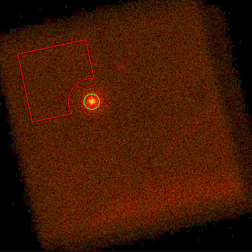
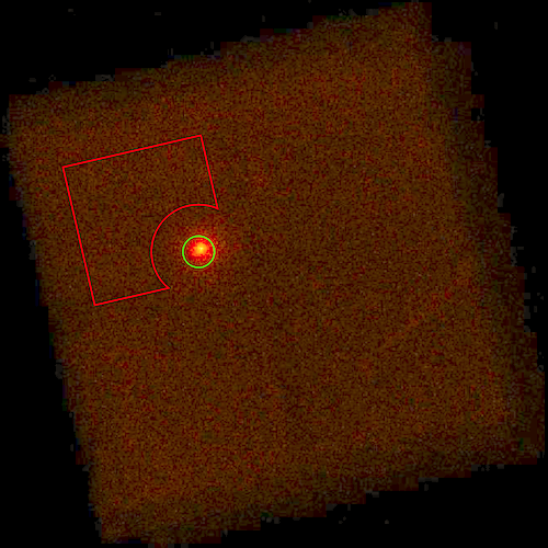
Figure 1: NuSTAR images showing the source extraction regions (green) and background regions (red) for FPMA (left) and FPMB (right). We only show the observation from 2014 April 22 because other observations are similar. The intensity scales are approximately linear and have been slightly offset to better show the background. The pixel size is $2\farcs{}46\times 2\farcs{}46$ and the FoV is approximately $13\arcmin{}\times{}13\arcmin$. North is up and east is left.

The NuSTAR telescope has an energy range of 3–78.4 keV and an angular resolution of 18″ (full width at half maximum; FWHM). The spatial resolution is insufficient to resolve the ER (${\sim}$1″) but clearly separates SN 1987A from any other sources. The energy resolution has a FWHM response of 0.4 keV at 10 keV and 0.9 keV at 60 keV. This spectral resolution allows for separation of isolated lines and line complexes from the continuum, but does not resolve finer structures or crowded spectral regions. NuSTAR has two mirror assemblies and two corresponding focal plane CCD modules (FPMs), referred to as FPMA and FPMB. The two parallel setups are practically identical but all data are analyzed separately and only combined for presentation purposes.

We use all on-axis NuSTAR observations of SN 1987A (Table 1), which constitute a total exposure time of 3.3 Ms. The majority of the data are from 2012–2014. These were previously used to study the radioactive ⁴⁴Ti lines (Boggs et al., 2015) and the continuum (Greco et al., 2021). To complement these data, we obtained new observations in May 2020, which allow us to study the recent temporal evolution. There are 17 individual observations in total, but these constitute eight groups of observations that are quasi-simultaneous (within two weeks, see Table 1). Henceforth, the observations within each group are treated as simultaneous, but the data are not combined except for presentation purposes.

The NuSTAR data reduction largely follows standard procedures. To reduce the data, we use NuSTARDAS 1.9.2 and NuSTAR CALDB version 20200726. First, calibrations and filters are applied using the nupipeline task. The exposures are filtered for passages through the South Atlantic Anomaly. This is a trade-off between exposure time and background. We check the SAA filter reports and use the options saacalc=1, saamode=strict, and tentacle=yes.

Spectra are then generated using the standard task nuproducts. Source counts are extracted from a circular region centered on SN 1987A, shown in Figure 1. We choose a radius of 30″, which is recommended for weaker sources by the NuSTAR Observatory Guide. This results in an encircled energy fraction of approximately 50 %. SN 1987A is relatively weak above 8 keV, which is the energy range that is most important for the analysis. Background regions are selected from the same CCD chip as the source. The vicinity of SN 1987A is free of strong NuSTAR sources, but bright X-ray sources outside the field of view (FoV) introduce stray light into the FoV (Madsen et al., 2017). In general, we aim to select background regions that are squares with sides of $4.5$′, while excluding a region around SN 1987A and stray light. The excluded region around SN 1987A is a circle with a radius of 90″ (see Figure 1).

We limit the energy range used for the continuum analysis to 3–24 keV. Both the flux and effective area quickly decrease toward higher energies, resulting in a signal-to-background ratio (S/B) lower than $0.3$. The low S/B above 24 keV results in a very high sensitivity to background systematics. Finally, the spectra are grouped to at least 25 counts per bin.

2.2 XMM-Newton

Table 2: XMM-Newton Observations

Obs. ID	Start Date	Epoch	RGS Exp.	pn Exp.	$C_{\text{RGS1}}$	$C_{\text{RGS2}}$	$C_{\text{pn}}$	NuSTAR Groups
	(YYYY-mm-dd)	(d)	(ks)	(ks)
0144530101	2003-05-10	1,5920	112(113)	59(107)	2996	3698	21,122	. $\cdots$
0406840301	2007-01-17	1,7268	082(111)	64(107)	5682	9030	91,386	. $\cdots$
0506220101	2008-01-11	1,7627	114(115)	70(110)	10,169	15,965	136,480	. $\cdots$
0556350101	2009-01-30	1,8012	090(102)	68(100)	10,258	15,503	164,945	. $\cdots$
0601200101	2009-12-11	1,8327	092(92)0	77(90)0	11,689	17,587	212,221	. $\cdots$
0650420101	2010-12-12	1,8693	066(66)0	51(64)0	9162	14,248	157,450	. $\cdots$
0671080101	2011-12-02	1,9048	075(82)0	62(81)0	11,156	17,346	213,257	. $\cdots$
0690510101	2012-12-11	1,9423	070(70)0	60(68)0	10,663	16,665	212,129	1–4
0743790101	2014-11-29	10,141	073(80)0	57(78)0	10,827	17,174	210,278	5–7
0763620101	2015-11-15	10,492	066(66)0	54(64)0	9558	15,084	195,380	. $\cdots$
0783250201	2016-11-02	10,845	074(74)0	48(72)0	10,416	16,159	176,047	. $\cdots$
0804980201	2017-10-15	11,192	072(79)0	34(78)0	9458	14,983	120,854	. $\cdots$
0831810101	2019-11-27	11,965	035(35)0	19(32)0	3925	6303	63,847	8

Note. — The net source counts in the different instruments are given by $C_{\mathrm{RGS1}}$, $C_{\mathrm{RGS2}}$, and $C_{\mathrm{pn}}$. All counts are for the standard energy ranges we use for the analysis (see text). The RGS counts are for 1st order only. The differences between RGS1 and RGS2 are primarily driven by the different non-operational CCDs. The total counts in the 2nd order spectra are 45 % of the 1st order counts for RGS1 and 26 % for RGS2.

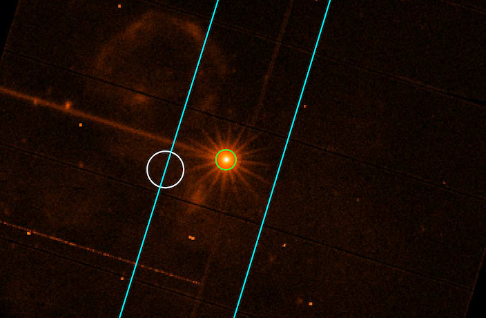
Figure 2: XMM-Newton/pn image showing the source region (green), background region (white), and RGS FoV (cyan). The cyan lines are parallel with the dispersion direction. We only show the observation from 2014 November 29 because other observations are similar. The intensity scale is logarithmic and white corresponds to ${\sim}$24,000 counts per pixel. The pixel size is $4\arcsec\times{}4\arcsec{}$ and the FoV of the image is approximately $27\arcmin{}\times{}18\arcmin$. North is up and east is left.

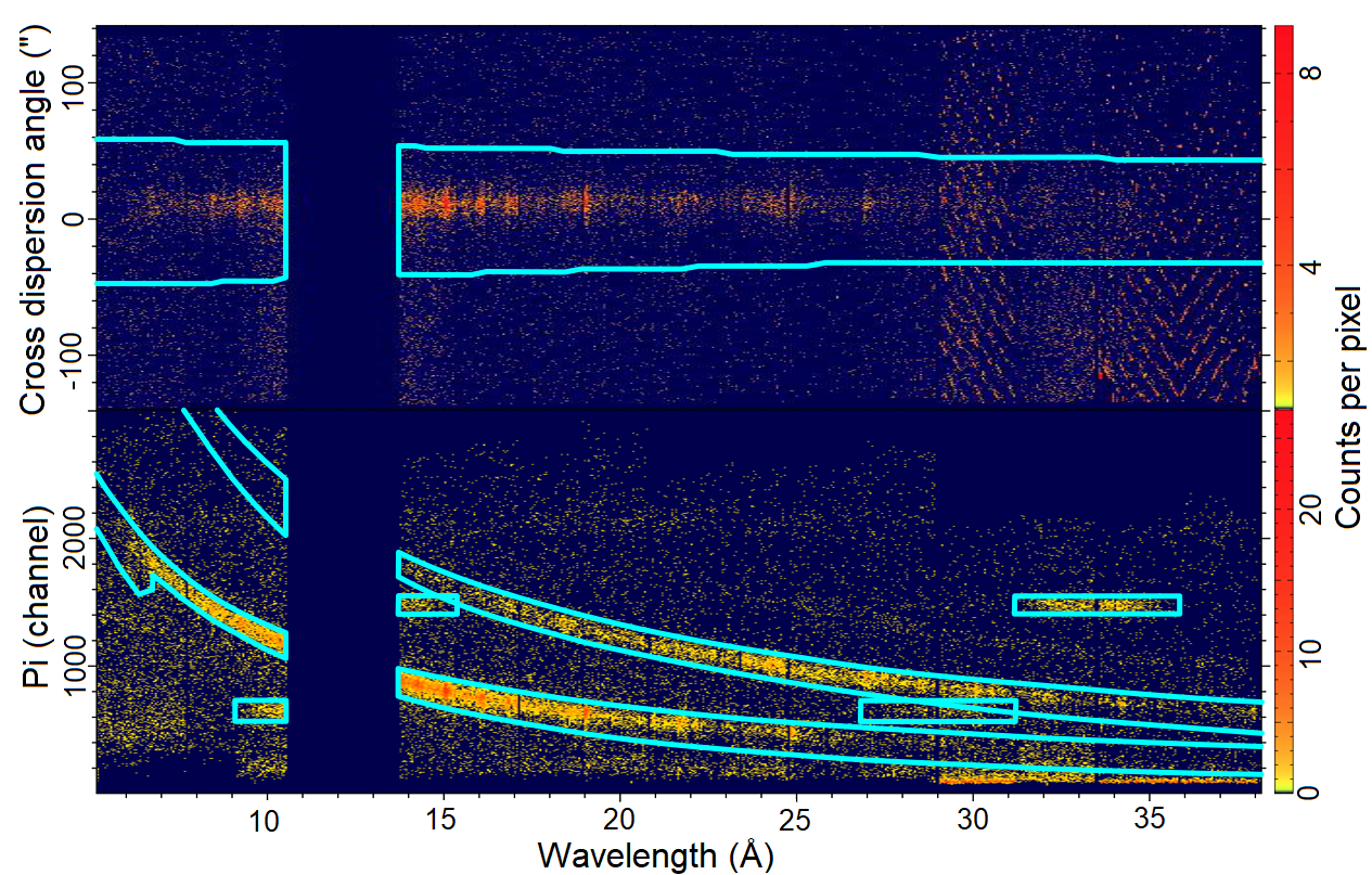
Figure 3: XMM-Newton/RGS1 images showing a 1-dimensional dispersed image in the upper panel and a PI-dispersion angle plot (banana plot) in the lower panel. The cyan regions in the upper panel are the source regions. The curved regions in the lower panel are source regions (1st and 2nd order) while the four rectangular regions show excluded areas (containing calibration sources). The spatial background region covers the entire exposed surface of the focal plane, except for a buffer zone around the source. We only show the observation from 2014 November 29 because other observations are similar.

XMM-Newton operates six instruments in parallel: the pn CCD (Strüder et al., 2001); MOS1 and MOS2 (Turner et al., 2001); two grating spectrometers (den Herder et al., 2001); and the optical monitor (Mason et al., 2001). Here, we focus on the pn CCD and the reflection grating spectrometers (RGSs). The pn camera covers 0.3–10 keV with a spectral resolution of $E/\Delta E\sim$ 20–50, which is comparable to the NuSTAR energy resolution. The RGSs cover 0.35–2.5 keV and provide $E/\Delta E\sim$ 200–600, which is sufficient to resolve the large number of lines in this energy range. The angular resolution is approximately 6″ (FWHM) for both pn and the cross-dispersion direction of the RGSs, which does not resolve the ER. The RGS apertures extend across the entire 30′ FoV along the dispersion direction, but the effective area decreases quickly as a function of off-axis angle. We verified that no other sources are confused with SN 1987A. Contamination along the dispersion direction of the RGSs can be identified by comparing the dispersion angle to the energy estimate from the RGS CCD readouts.

We primarily focus on the most recent XMM-Newton observations for the joint NuSTAR-XMM analysis, but include 13 publicly available XMM-Newton observations in total for a longer temporal baseline (Table 2). Due to modest levels of pile-up (detailed below), we only use CCD data from the pn CCD, and not the MOS CCDs (Turner et al., 2001). Pile-up is not present in the RGS data.

For the data reduction, we use XMM SAS 18.0.0 (Gabriel et al., 2004) with XMM CCF updated on 2020 August 3. Most steps of the data reduction follow default standards. We reprocess the data with the latest calibrations and filter the data for high-background intervals (Table 2).

For the pn data, we extract source spectra from a circular region centered on SN 1987A with a radius of 30″, shown in Figure 2. This is a typical source extraction radius and results in an encircled energy of 80–90 % depending on energy (lower for higher energies). A larger source radius would only increase the signal marginally while lowering the S/B. For reference, a source radius of 90″ results in an encircled energy of 90–95 %, while increasing the background from ${\sim}$1 % to almost 10 %. Backgrounds are extracted from circular regions from the same CCD chip (#4) with radii of approximately 60″ (Figure 2). The very high S/B implies that the choice of background has a negligible impact on the analysis. The RGS spectra are constructed using the default source and background regions. A heliocentric correction to the photon energies is also applied to the RGS data by default.

We pay special attention to pile-up in the CCD spectra. Pile-up occurs when multiple photons hit the same or adjacent pixels within the same readout frame. The results are that some photons are rejected as invalid events, and an artificial hardening of the spectrum as the energies of multiple photons are combined. Pile-up affects approximately 5 % of the events when the photon flux peaks around the year 2014. This is estimated using the task epatplot, which compares the observed event patterns with expected pattern distributions. Even though the magnitude of the effect is low, it could significantly affect the fits. The bins with the most photons have statistical uncertainties as low as 1 %. We use the task rmfgen to produce response matrix files (RMFs) that account for pile-up, which is enabled by the option correctforpileup=yes. The ancillary response files (ARFs) are then generated using the standard task arfgen.

The CCD spectra are grouped to a minimum of 25 counts per bin using specgroup. Additionally, we impose a minimum bin size corresponding to $1/3$ of the energy resolution FWHM using the parameter oversample=3. The RGS spectra are also binned to a minimum of 25 counts per bin, but using the general task grppha. The large number of photons allows for this binning without significantly downsampling the energy resolutions of the RGSs.

We limit the energy range of the pn data to 0.8–10 keV. The lower bound of 0.8 keV is higher than the lower calibration limit of 0.3 keV. We ignore data below 0.8 keV because of inconsistencies between the pn and RGS spectra of up to 5 % close to strong lines, which are likely due to calibration uncertainties. The pn spectral bins have individual statistical uncertainties as low as $\pm 1$ % at low energies, which implies that slight calibration issues could significantly reduce the goodness of fit. The calibration accuracy is known to decrease toward lower energies (Plucinsky et al. 2008, 2017; see also Figures D.1 and D.2), possibly due to the lowest-energy internal calibration line of pn being at 1.5 keV (Strüder et al., 2001). We choose the 0.8 keV limit as a trade-off between using as much data as possible and introducing calibration tensions into the fits.

We use RGS data from both RGS1 and RGS2, and 1st and 2nd order. An RGS1 image showing the dispersed data is provided in Figure 3. The two 1st order spectra cover the energy range from 0.45 to 1.95 keV, whereas the 2nd order spectra range from 0.70 to 1.95 keV. The low energy cutoff of 0.45 keV implies that we include the strong N vii Ly$\alpha$ line at 0.50 keV, below which very few photons are detected. Additionally, the parts of the RGS spectra that coincide with non-operational CCDs are excluded.

3 Analysis

We use XSPEC 12.11.0 for spectral fitting and use the photoabsorption cross sections of Verner & Yakovlev (1995). We follow the XSPEC convention of the photon index $\Gamma$ being given by $N\propto E^{-\Gamma}$, where $N$ is the photon flux density and $E$ the photon energy. Furthermore, the spectral binning of at least 25 counts per bin allows for the use of $\chi^{2}$ statistics.

Confidence intervals are computed using the error command in XSPEC. All intervals are 90 % unless otherwise stated, whereas one-sided limits are 3$\sigma{}$. The error command varies the parameters until the $\chi^{2}$ value reaches a given threshold. We adopt a critical value of 2.706, which is commonly used in X-ray analyses. However, we stress that this technically only represents the 90 % interval for one parameter of interest (Avni, 1976; Lampton et al., 1976; Cash, 1976). The same argument applies to the 3$\sigma{}$ limits, for which we use a corresponding threshold of 7.740.

We use different combinations of data sets for different purposes. For the flux estimates, we prioritize good fits to individual epochs. Therefore, we only use NuSTAR data for NuSTAR fluxes, and pn and RGS data for XMM-Newton fluxes. For the spectral analysis, we perform joint fits to NuSTAR and RGS data. We omit the XMM-Newton/pn data in these fits due to calibration uncertainties, which could introduce systematic effects. The significance of the calibration uncertainties is exacerbated by the large number of photons in the pn data. We discuss the magnitude and characteristics of the instrumental uncertainties further in Appendix C. Furthermore, Appendix D investigates the effects of including pn in the data analysis, as well as explores a number of other alternatives for how to manage the systematic uncertainties. The primary conclusion is that different choices affect the best-fit values quantitatively but the qualitative scientific conclusions remain unchanged.

For all fits, we leave a free cross-normalization constant between different instruments to accommodate calibration uncertainties. The cross-normalizations also allow for some freedom between the NuSTAR and XMM-Newton observations, which are separated in time. These constants are generally fitted to values within 0.9–1.1, with most values being close to unity. For some fits, the constants deviate by more than 10 % form unity, but this is predominantly due to the time difference between some of the NuSTAR and XMM-Newton observations. This shows that the cross-normalizations primarily capture calibration uncertainties and to some extent also the temporal evolution between non-simultaneous observations. Importantly, these constants do not drift to unreasonable values, which would indicate problems with the fits.

3.1 Spectral Modeling

For spectral modeling, we consistently use the same base model unless otherwise stated. It consists of an absorption component, a Gaussian smoothing kernel, and three shocked plasma components. We use the Tuebingen-Boulder interstellar medium (ISM) absorption model (TBabs; Wilms et al. 2000), gsmooth for smoothing, and vpshock for the plasma emission. We use three duplicates of the shock component to properly capture the range of temperatures that contribute to the spectrum in the 0.45–24 keV range (Section 4.2 and Appendix D). Below, we describe the components in more detail.

The absorption component has only one free parameter, which is the H column density ($N_{\mathrm{H}}$). We stress that this is the total H density, including both atomic H and molecular H₂ (Willingale et al., 2013). Solely for the absorption, we adopt the Milky Way ISM abundances of Wilms et al. (2000). Implications of this on the estimated $N_{\mathrm{H}}$ are discussed in Section 3.2.

The Gaussian smoothing represents the broadening of the spectral lines due to the bulk and turbulent motion of the emitting plasma (Appendix of Dewey et al. 2012). The amount of Doppler blurring in units of energy is proportional to the energy. This implies that the exponent ($\alpha$) for the gsmooth energy dependence is always frozen to 1. Thus, the only free parameter of the smoothing component is the magnitude of the blurring measured by $\sigma{}$ of the Gaussian kernel. Freezing $\alpha$ to 1 implicitly assumes that the emission is produced by gas with the same bulk velocity. Neither assumption is likely strictly fulfilled. However, we fix it at 1 since we find negligible improvements when leaving it as a free parameter.

The vpshock component (Borkowski et al., 2001) is based on calculations of X-ray spectra using a SN blast-wave model. The main parameters are the shock temperature ($T$), ionization age ($\tau$), and emission measure (EM). The EM is implemented as the XSPEC normalization but can be converted to an EM using a distance of 51.2 kpc to SN 1987A (Panagia et al., 1991; Mitchell et al., 2002). The vpshock model also allows for variable abundances (Section 3.2). The model assumes an adiabatic, one-dimensional plasma shock with constant temperature propagating into a uniform CSM. This is clearly oversimplified compared to the complex ER structure. At X-ray energies below ${\sim}$2 keV, the shocks producing the emission in SN 1987A are also likely radiative and not adiabatic (Pun et al., 2002; Gröningsson et al., 2008). A radiative shock produces softer emission compared to an adiabatic shock at the same temperature, as well as different line ratios (Nymark et al., 2006). These effects add additional systematic uncertainties into the absorption and abundance estimates discussed below. The vpshock model also assumes a Maxwellian electron velocity distribution and no cosmic ray modifications. Accelerated cosmic rays could diffuse upstream and form a shock precursor that decelerates the gas ahead of the shock (Borkowski et al., 2001). This would lead to a lower temperature than in the standard, non-modified shock of the same velocity.

3.2 Fixed Parameters

Table 3: Fixed Parameters

Parameter	Value
$N_{\mathrm{H}}$	$2.60_{-0.05}^{+0.05}\times{}10^{21}$ cm-2
$\sigma(1\mathrm{~{}keV})$0000000000000	$1.1\pm 0.1$ eV
$z$	$(9\pm{}5)\times{}10^{-4}$
$V_{\mathrm{r}}(z)$	$260\pm{}120$ km s-1

Note. — Parameters determined from simultaneous fits to three XMM-Newton observations. They are kept fixed in all other fits. The recession velocity ($V_{\mathrm{r}}$) is inferred from the fitted redshift.

There are a number of spectral parameters that we keep constant throughout the time range spanned by our observations. These parameters are the ISM absorption column density, line broadening, elemental abundances, and redshift (Tables 3 and 3.2). We initially perform a fit to determine these parameters. This is done to avoid having to fit all spectra simultaneously with an excessive number of free parameters. All these constant parameters are primarily constrained by the RGS spectra, and to some extent the pn spectra. Thus, for this particular fit, we simultaneously fit the model to three XMM-Newton observations: 9423; 10,141; and 11,192 d (Table 2). The choice of these observations offer a trade-off between exposure time, covering the NuSTAR epochs, and a short enough time range during which spectral variations are moderate.

For this fit, we tie all parameters that are expected to be constant. Each observation epoch consists of one pn spectrum and four RGS spectra. Among these five spectra, the plasma temperature, ionization age, and EM are tied across the instruments. The setup is the same for each of the three plasma components. These plasma parameters are not tied between observations since they evolve significantly with time. The cross-normalization constant is frozen to 1.0 for the 1st order RGS1 spectra and left free for the other spectra from the same observation. The global fit statistic is $\chi^{2}=5459$ for 4617 degrees of freedom (DoF), with relatively similar goodnesses of fit for different spectra.

From the fit, we obtain a best-fit $N_{\mathrm{H}}$ of $2.60_{-0.05}^{+0.05}\times{}10^{21}$ cm^-2. This is low compared to estimates of the Galactic $N_{\mathrm{H}}$ from H i surveys. For example, Willingale et al. (2013) report $4.09\times{}10^{21}$ cm^-2 and HI4PI Collaboration et al. (2016) $3.86\times{}10^{21}$ cm^-2 (assuming 20 % of H₂ for the latter), which are too high to result in statistically acceptable fits to the XMM-Newton (mainly RGS) data. Additionally, optical extinction estimates show that the LMC contribution is greater than the Milky Way contribution (Fitzpatrick & Walborn, 1990; France et al., 2011). This implies that the X-ray absorption to SN 1987A should be even higher than the Galactic H i estimates.

There are two likely contributing factors to our apparent underestimation of $N_{\mathrm{H}}$. First, the employed adiabatic model (Section 3.1) produces harder spectra than radiative shocks (Nymark et al., 2006). This could artificially suppress $N_{\mathrm{H}}$ in order to produce a softer absorbed spectrum. Second, we use the Galactic abundances of Wilms et al. (2000) for the absorption component to reduce complexity. In reality, the gas along the line of sight could be of lower metallicity, especially the LMC absorption component. This would also have the effect of lowering the fitted $N_{\mathrm{H}}$ to compensate for an assumed metallicity that is too high. However, we note that our X-ray estimate of $N_{\mathrm{H}}$ is comparable to those obtained by other X-ray analyses. For example, Zhekov et al. (2009) report $1.44_{-0.12}^{+0.16}\times{}10^{21}$ cm^-2 and (Park et al., 2006) report $2.35_{-0.08}^{+0.09}\times{}10^{21}$ cm^-2. These differences are small in light of the different modeling techniques and instruments used. In summary, we conclude that our best-fit $N_{\mathrm{H}}$ of $2.60\times{}10^{21}$ cm^-2 may be underestimated due to systematic uncertainties, but we use it in all subsequent fits since it provides the best fit quality and is comparable to previous X-ray estimates.

The best-fit Doppler blur, measured as $\sigma$ of the Gaussian smoothing kernel, is $1.1\pm 0.1$ eV at 1 keV. For reference, Dewey et al. (2012) find a value of 1.0 eV in their analysis of RGS data.

The best-fit redshift with statistical uncertainties obtained in XSPEC is $8.81_{-0.01}^{+0.02}\times{}10^{-4}$. The total uncertainty is dominated by the RGS absolute calibration of $\pm{}5$ mÅ ($4\times{}10^{-4}$ keV at 1 keV). Therefore, we adopt $(9\pm{}5)\times{}10^{-4}$ as the redshift estimate from our X-ray data, which corresponds to a recession velocity of $260\pm{}120$ km s^-1. This is consistent with an optical estimate of 286.74 km s^-1 (Gröningsson et al., 2008). However, we note that these values represent redshifts integrated over velocities along the line of sight and the entire ER, which has spatial differences in the relative brightness in X-ray and optical. Therefore, it is likely that the X-ray and optical redshifts are truly slightly different. For our purpose, we prioritize a good fit to the data and choose to use the value we obtain from the X-ray fit.

Table 4: ER Abundances

Element	Abundance	$A/A_{\mathrm{ISM}}$	$A/A_{\mathrm{LMC}}$	Ref.
	(dex)
H	$\equiv{}12$	$\equiv{}1$	$\equiv{}1$	$\cdots$
He	$11.40$	$2.56$	$2.87$	1
C	$7.51$	$0.13$	$0.29$	1
N	$8.30_{-0.02}^{+0.03}$	$2.65_{-0.12}^{+0.20}$	$14.58_{-0.68}^{+1.08}$	$\cdots$
O	$8.26_{-0.02}^{+0.01}$	$0.37_{-0.01}^{+0.01}$	$0.82_{-0.03}^{+0.03}$	$\cdots$
Ne	$7.82_{-0.01}^{+0.01}$	$0.76_{-0.02}^{+0.02}$	$1.63_{-0.03}^{+0.03}$	$\cdots$
Mg	$7.28_{-0.01}^{+0.01}$	$0.76_{-0.02}^{+0.02}$	$0.65_{-0.02}^{+0.01}$	$\cdots$
Si	$7.28_{-0.01}^{+0.01}$	$1.03_{-0.02}^{+0.02}$	$0.30_{-0.01}^{+0.01}$	$\cdots$
S	$7.02_{-0.02}^{+0.02}$	$0.85_{-0.04}^{+0.04}$	$2.08_{-0.11}^{+0.10}$	$\cdots$
Ar	$6.23$	$0.66$	$0.87$	2
Ca	$5.89$	$0.49$	$1.00$	3
Fe	$7.02_{-0.004}^{+0.01}$	$0.39_{-0.004}^{+0.01}$	$0.62_{-0.01}^{+0.02}$	$\cdots$
Ni	$6.04$	$0.98$	$1.00$	3

References. — (1) Sect. 3.1 of Lundqvist & Fransson (1996), (2) Table 7 of Mattila et al. (2010); (3) Table 1 of Russell & Dopita (1992).

Note. — Values with error bars were determined from our fits, whereas the others are taken from the provided references.

All fitted abundances are provided in Table 3.2. It also includes abundances of He, C, Ar, Ca, and Ni, which are taken from the literature. These abundances cannot be fitted for because they are very weakly constrained by the X-ray data. Overall, the fitted abundances are largely within the ranges of values reported by previous studies (Lundqvist & Fransson, 1996; Mattila et al., 2010; Sturm et al., 2010; Dewey et al., 2012; Bray et al., 2020). For example, our estimated Fe abundance of $0.62_{-0.01}^{+0.02}$ relative to the LMC abundance can be compared to other X-ray estimates (all expressed relative to the LMC abundance): $0.55_{-0.03}^{+0.03}$ (Zhekov et al., 2009), $0.36_{-0.01}^{+0.01}$ (Sturm et al., 2010), $0.62_{-0.01}^{+0.02}$ (Dewey et al., 2012), and $0.44_{-0.03}^{+0.03}$ (Bray et al., 2020). However, we caution that all X-ray estimates of the abundances likely suffer from similar significant systematic uncertainties due to the modeling and absorption uncertainties described above.

We leave the abundances of all trace elements to their default values, namely 1.0 relative to our adopted ISM abundances. All fits are insensitive to these trace elements. We test this by setting the abundances of all trace elements to 0.0 using the command NEI_TRACE_ABUND. The $\chi^{2}$ value fluctuates by a few and all fitted parameters are practically unchanged.

3.3 Flux Estimation

To estimate fluxes, we use the model and parameters described above. The model is fitted simultaneously to all spectra within the groups of NuSTAR observations and within each XMM-Newton observation. The free parameters are the temperatures, ionization ages, and EMs for each of the shock components, and a free cross-normalization between the instruments. The NuSTAR data are unable to robustly constrain the coolest plasma component. Therefore, we freeze its parameters to the values from the fits to the XMM-Newton data that are closest in time. This component is almost completely below the lower energy limit of NuSTAR and does not affect the fluxes significantly. The parameters of each plasma component that are fitted for are tied across instruments since the spectra are (quasi-)simultaneous. The average reduced fit statistic is $\chi^{2}_{\mathrm{red}}=0.93$ with an average of 347 DoF for the NuSTAR epochs. The corresponding numbers for the XMM-Newton observations are $\chi^{2}_{\mathrm{red}}=1.2$ and 1555 DoF.

We measure fluxes using the XSPEC component cflux, which has a parameter that corresponds to the flux. After fitting the model, the cross-calibration constant is replaced by cflux and the model is refitted. This results in a flux estimate from each spectrum, which also captures the calibration differences between the instruments. We report the weighted average as the best-estimate flux, but the individual flux measurements provide a handle on the level of systematics (Appendix C). All reported fluxes are observed (not correcting for ISM absorption) due to the uncertain amount of absorption and to allow for comparisons with previous studies.

3.4 Continuous Temperature Model Setup

In addition to the standard model, we use a more complex model for the joint NuSTAR and RGS spectral analysis. It is the same as the base model except that the three shock components are replaced by a distribution of shocks over a continuous temperature interval (Zhekov et al., 2006, 2009), analogous to the XSPEC model c6pvmkl (Lemen et al., 1989; Singh et al., 1996). The distribution of shock EMs is given by

$$\phi{}=\delta_{1}\exp\!\left(\sum_{i=0}^{6}a_{i}P_{i}\!\left(T^{\prime}\right)\right),$$ (1)

where $\delta_{1}$ is a normalization, $a_{i}$ are the fitting coefficients, and $P_{i}$ is the Chebyshev polynomial of the first kind of order $i$. The polynomial argument $T^{\prime}{}$ is a rescaling of the plasma temperature $T$ such the temperature interval $0.125$ to $10$ keV is mapped logarithmically to the domain $-1$ to $1$. The seemingly arbitrary parametrization of $\phi$ reduces the number of free parameters and makes the fitting better conditioned. Numerically, the continuous temperature is implemented as 28 vpshock components with $T$ logarithmically spaced between 0.125 and 10 keV. To further reduce the number of free parameters, we parametrize the ionization age of each shock component as

$$\tau=\delta_{2}T_{\mathrm{keV}}^{p},$$ (2)

where $T_{\mathrm{keV}}$ is the temperature in keV, and both the normalization $\delta_{2}$ and power-law (PL) index $p$ are fitted for. To summarize, this means that we fit a shock with a continuous distribution of $T$ using ten free parameters: two normalizations, seven polynomial coefficients, and the ionization PL index.

The primary advantage of this continuous model is the ability to capture the complex underlying physics. It has only one more free parameter than the three-shock standard model. The tradeoff is increased freedom in temperature at the cost of a more constrained ionization age. Importantly, the continuous model allows for the possibility to separate different components by analyzing the EM distribution. Statistically, typical improvements compared to the standard three-shock model is $\Delta\chi^{2}=-20$ for an average number of DoF of ${\sim}$1800. However, the number of shock components in ordinary models is arbitrary and harder to interpret physically. A priori, it is not clear how each discrete model component translates to physical components.

4 Results

4.1 Light Curves

Table 5: NuSTAR Fluxes

Group	Epoch	$F_{\text{3--8}}$	$F_{\text{10--24}}$	$F_{\text{3--24}}$
	(d)	($10^{-13}$ erg s-1 cm-2)	($10^{-13}$ erg s-1 cm-2)	($10^{-13}$ erg s-1 cm-2)
1	9331	$10.5_{-0.2}^{+0.2}\pm 0.8$	$1.78_{-0.07}^{+0.07}\pm 0.14$	$13.3_{-0.2}^{+0.2}\pm 1.1$
2	9372	$11.3_{-0.2}^{+0.3}\pm 0.9$	$1.67_{-0.10}^{+0.09}\pm 0.13$	$14.0_{-0.3}^{+0.3}\pm 1.1$
3	9424	$11.0_{-0.3}^{+0.3}\pm 0.9$	$1.67_{-0.11}^{+0.12}\pm 0.13$	$13.7_{-0.3}^{+0.3}\pm 1.1$
4	9623	$11.2_{-0.2}^{+0.2}\pm 0.9$	$1.73_{-0.08}^{+0.08}\pm 0.14$	$14.0_{-0.2}^{+0.2}\pm 1.1$
5	9920	$12.6_{-0.2}^{+0.2}\pm 1.0$	$1.82_{-0.09}^{+0.07}\pm 0.15$	$15.6_{-0.2}^{+0.2}\pm 1.2$
6	9976	$11.7_{-0.2}^{+0.2}\pm 0.9$	$1.90_{-0.08}^{+0.09}\pm 0.15$	$14.7_{-0.3}^{+0.3}\pm 1.2$
7	10,021	$12.1_{-0.2}^{+0.2}\pm 1.0$	$1.69_{-0.08}^{+0.08}\pm 0.13$	$15.0_{-0.2}^{+0.2}\pm 1.2$
8	12,140	$16.2_{-0.3}^{+0.3}\pm 1.3$	$1.92_{-0.11}^{+0.08}\pm 0.15$	$19.6_{-0.3}^{+0.3}\pm 1.6$

Note. — The flux $F_{a\text{--}b}$ denotes the flux from $a$ to $b$ keV. Asymmetric error bars are statistical and the symmetric uncertainties are systematic (Appendix C).

We report observed fluxes in a number of different energy bands. For NuSTAR, we study the 3–8, 10–24, and 3–24 keV ranges. The 3–8 keV is the “hard” band in XMM-Newton and Chandra contexts. XMM-Newton fluxes are provided in the 0.5–2, 3–8, and 0.5–8 keV bands, in line with previous studies (e.g. Frank et al. 2016). Additionally, we also compute the 0.45–0.7 keV flux, which is dominated by N vii and O viii Ly$\alpha$. All NuSTAR fluxes are provided in Table 5, whereas the XMM-Newton fluxes are provided in Appendix E.

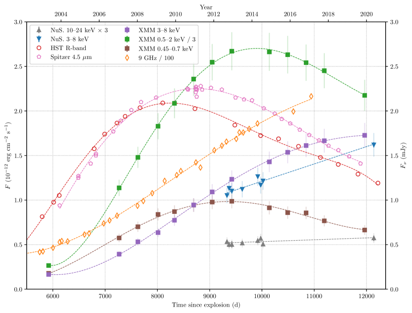
Figure 4: NuSTAR (triangles), XMM-Newton (squares), HST R-band (circles; Larsson et al. 2019), Spitzer $4.5$ µm (pentagons; Arendt et al. 2020), and 9 GHz radio light curves (diamonds; Cendes et al. 2018). Solid symbols represent X-ray data and hollow symbols show other wavelengths. The two $y$-axes are not equivalent. The right axis applies to the Spitzer and radio data, whereas the left applies to the other data. We note that the 0.5–2 keV, 10–24 keV, and radio data have been rescaled for clarity as shown in the legend. The dashed lines are polynomial fits to guide the eye. The fits to NuSTAR data are of first order, while the others are fourth or fifth order polynomials. The solid X-ray error bars are statistical (often smaller than the markers) and the semi-transparent error bars approximately represent the systematic uncertainties (Appendix C).

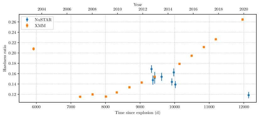
Figure 5: Hardness ratios, defined as the ratio in a hard over a soft band. For NuSTAR, the hard band is 10–24 keV and soft 3–8 keV. The soft XMM-Newton range is 0.5–2 keV, whereas the hard is 3–8 keV. These error bars only include the statistical uncertainty since ratios are computed using homogeneous instrumental setups in each band.

The light curves are shown in Figure 4. In addition to NuSTAR and XMM-Newton, we show HST R-band (WFPC2/F675W, ACS/F625W, WFC3/F625W; Larsson et al. 2019), $4.5$ µm Spitzer (Arendt et al., 2020), and 9 GHz radio (Cendes et al., 2018) light curves. The two most recent HST data points are previously unpublished, but are computed using the same methods as the other data points and include only the ER emission. The observations were obtained on 2019 July 22 (11,837 d) and 2020 August 6 (12,218 d).

It is apparent that the 3–8 keV light curves and the 9 GHz radio show similar temporal evolutions. In contrast, the 10–24 keV component increases at a lower relative rate. We note that the 0.5–2 keV flux clearly starts decreasing after around 10,000 d, and that the rise of the 3–8 keV flux slows slightly after 11,000 d. This is also reported by Sun et al. (2021) using XMM-Newton data, as well as in a preliminary study of recent Chandra observations (Ravi, 2019). These spectral changes are captured by the hardness ratios shown in Figure 5. This illustrates how the 3–8 keV flux becomes increasingly dominant, with the spectra hardening in the XMM-Newton energy range and softening in the NuSTAR range. Finally, we note that the 0.45–0.7 keV evolution is more strongly correlated with the decaying optical flux than the 0.5–2 keV light curve.

The offset of ${\sim}$10–15 % between the NuSTAR and XMM-Newton 3–8 keV light curves reveal a systematic difference (Appendix C). However, for our conclusions, we focus on the evolution as observed by the same instrument, which should be free from large systematics.

There are indications of variability of approximately 5 % between the NuSTAR epochs on timescales of a few weeks (among groups 1–3 and 5–7). We caution that these variations might be due to observational uncertainties, instrumental origin, or the data reduction process.

4.2 Standard Shock Model

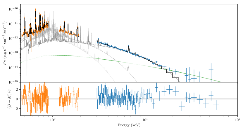
Figure 6: Upper panel: Unfolded observed spectra (absorbed but corrected for the instrument responses) from NuSTAR (blue), RGS (orange), and the model (black) in flux space. The NuSTAR data are plotted up to 65 keV (just below the ⁴⁴Ti lines), but the fits are performed using only data up to 24 keV. For visual clarity, we show the sum of the six individual NuSTAR exposures from the first epoch at 9331 d and only the 1st order RGS1 data from 9423 d. Both the NuSTAR and RGS data are also rebinned (represented by the horizontal error bars). The vertical error bars are 1$\sigma{}$ intervals. The thin dashed lines are the low- (light gray), mid- (gray), and high-temperature (dark gray) shock components that constitute the model. The dotted green line is the non-thermal synchrotron prediction from Berezhko et al. (2015). It is not part of the fitted model, but is overplotted for reference. The synchrotron component is shown for 9280 d, close to the predicted time of the synchrotron maximum. Although the green synchrotron prediction appears to match two bins around 20 keV, an additional component is not statistically motivated (Section 4.5) and the synchrotron prediction is only marginally consistent with the data above 24 keV (Section 5.4). Lower panel: Normalized residuals between data and model. This difference is computed in count space, implying that the model is forward-folded and then compared to the data. The non-thermal synchrotron component (dotted green line) is not part of the model used for computing the residuals.

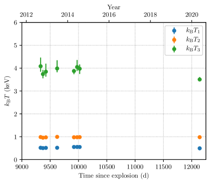
Figure 7: Evolution of the best-fit temperatures of the standard three-shock model. The subscripts denote the different shock components: low (1), mid (2), and high (3) temperature. The error bars for the low- and mid-temperature components are small compared to the markers (Tables 11 and 12).

We fit the spectral model with three shock components to all NuSTAR and RGS data sets. Figure 6 shows the best-fit model, its three components, and data from the first NuSTAR epoch (9331 d). The standard model provides an adequate fit and no additional component is statistically necessary (Section 4.5).

We verify that the 0.45–24 keV spectrum cannot be adequately modeled by a two-shock component model. This worsens the average goodness of fit to the combined NuSTAR and RGS data by $\Delta\chi^{2}\approx{}320$ for ${\sim}$1800 DoF. We provide a much more extensive investigation of the effects of different set-ups for the spectral analysis in Appendix D.

Evolutions of the temperatures of the shock components are shown in Figure 7. Typical temperatures for the three components are 0.3, 0.9, and 4 keV. The only variation in best-fit temperature is a slight decrease of the hottest component at the last NuSTAR epoch (12,140 d).

For completeness, we provide all best-fit parameters, fluxes of shock components, and fit statistics in Appendix F. We caution that the ionization ages for the three components may be unreliable. This is most evident for the mid-temperature component, which has a pegged ionization age at all epochs (Table 11). In particular, there appears to be too much freedom in the fits when the ionization ages of the three components are completely free. It is also probable that the fitted ionization ages are sensitive to underlying model uncertainties (Section 3.1). The fitted parametrization (Eq. 2) of the ionization age used in the continuous shock model is likely more robust (Section 4.4).

4.3 The Fe K$\alpha$ Line

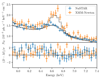
Figure 8: Spectral fits around the Fe K complex in count space. The panels are structured similarly to Figure 6. For visual clarity, the data shown are the sum of all NuSTAR data (blue crosses) and the sum of the eight XMM-Newton/pn observations after 8500 d. The summed data are not suited for detailed spectral fitting. Instead, we overplot the best-fit to the NuSTAR data at 9920 d, which is close to the average best-fit. The solid (NuSTAR) and dashed (XMM-Newton) black lines are the same underlying model, but produce different fluxes because of the different instrumental responses. We stress that the large amount of data (${\sim}$500 photons per bin in NuSTAR) makes even small flux and energy differences appear highly significant. The bin size is 0.04 keV for both NuSTAR and XMM-Newton. For reference, the absolute energy calibration around the Fe K complex is 0.04 keV for NuSTAR (Madsen et al., 2015) and 0.01 keV for XMM-Newton/pn.

Due to the importance of the Fe K lines, we show the integrated Fe K complex in Figure 8. The Fe K blend is clearly detected and implies that at least a significant fraction of the emission at high energies is thermal (see further Section 5.3). The observed line centroid in the NuSTAR data is ${\sim}$6.59 keV and ${\sim}$6.66 keV in the XMM-Newton data. We note that Sun et al. (2021) performed a more detailed, time-resolved analysis of the Fe line. They find that the lines centroid increases from around 6.60 keV at 8500 d to 6.67 keV at 12,000 d.

A line energy of 6.66 keV approximately corresponds to Fe xxiii, which is consistent with a thermal origin of temperature $>1$ keV (Makishima, 1986; Kallman et al., 2004). The identification as Fe xxiii is only indicative and the spectrum clearly has contributions from a range of ionization levels. For reference, Maggi et al. (2012) reported an emission-line centroid of $6.60\pm 0.01$ keV and a width of ${\sim}$100 eV. From this, they infer the presence of ionization stages from Fe xvii to Fe xxiv, which is in agreement with our result.

Our model spectrum is completely dominated by the 4 keV shock component at these energies (Figure 6) and it captures the line profile well. Previous, more careful XMM-Newton analyses of the Fe line have reported that there is a significant contribution of lower ionization levels around 6.5 keV, which is not captured by a thermal shock model (Sturm et al., 2010; Maggi et al., 2012). Maggi et al. (2012) suggested that this could originate from fluorescence from near-neutral Fe, including Fe in the unshocked ejecta. We do not investigate this in detail, but Figure 8 shows that any low-ionization contribution is clearly much weaker than the dominant component from the thermal shock model.

4.4 Continuous Shock Model

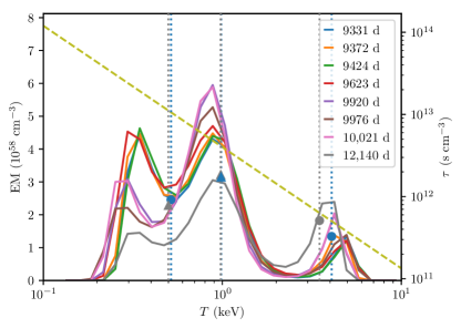
Figure 9: Results of the spectral analysis. Left axis: Solid lines are the fitted EM distributions (Eq. 1) for the continuous shock temperature model. Right axis: The dashed olive line is the parametrized ionization age (Eq. 2) from the continuous temperature fits. It is shown for the average $\delta_{2}$ and $p$ for visual clarity, but the $\tau$ parametrizations for the different NuSTAR epochs are similar. The vertical dotted lines are the temperatures for the first (blue; September 2012) and last (gray; May 2020) NuSTAR epochs that are obtained by fitting the standard model with three shock components. We note that the mid-temperature lines close to 1 keV are almost overlapping. The points are the fitted $\tau$ for the respective plasma components and the triangles are lower limits in cases where $\tau$ is unconstrained. All parameter values from the fits using three shock components are provided in Table 11.

In this section, we report the results of the continuous temperature shock model (Section 3.4). The EM distributions are shown in Figure 9. The distributions at all epochs are qualitatively similar, with three peaks at shock temperatures around 0.3, 0.9, and 4 keV. The isolated peak around 4 keV appears to be robustly separated from the lower-temperature components. The reduced $\chi^{2}$ for all fits are in the range 1.05–1.15, with an average number of DoF of 1685.

We caution that the apparent bimodality separating the 0.3 and 0.9 keV peaks is only marginally significant. We draw this conclusion because some fits using different initial conditions find solutions with a single, broad hump ranging from 0.3–1 keV. These solutions are only marginally statistically worse. Regardless of the detailed structure of the distribution below $2$ keV, it is still clear that there is a contribution from a broad range of temperatures in the range 0.3–0.9 keV. We reiterate that the shock model relies on a number of assumptions, which introduce additional uncertainties (Section 3.1). It is not computationally feasible to perform a formal error analysis for the EM distribution. Consequently, we note that some of the EM distribution variability between epochs could be insignificant. For analyzing the temporal evolution, the light curves (Section 4.1) and three-shock model fits (Section 4.2) are more robust.

The parametrized ionization age (Eq. 2) is a decreasing function of temperature at all epochs (Figure 9). The best-fit parameters are $\delta_{2}=4_{-2}^{+16}\times{}10^{12}$ s cm^-3 and $p=(-1.5)_{-1.3}^{+0.7}$. The ionization age is formally defined as the product of the remnant age and the density. For a remnant age of 10,000 d, the parameters above yield a density of $9[0.5$–$50]\times{}10^{4}$ cm^-3 at 0.3 keV, $6[2$–$20]\times{}10^{3}$ cm^-3 at 0.9 keV, and $4[2$–$6]\times{}10^{2}$ cm^-3 at 4 keV. The values quoted above are averages across the eight NuSTAR epochs and the intervals in brackets show the minimum and maximum values. As noted in Section 4.2, the free ionization ages for the standard three-shock model are poorly constrained by the fits. The fit of the parametrized ionization age for the continuous model discussed here is likely more robust, but we caution that systematics certainly are present at some level. In particular for shock temperatures as low as 0.3 keV, since these shocks are likely not adiabatic (Section 3.1).

Figure 9 also shows the best-fit temperatures for fits using the standard three-shock-component model. Only temperatures for the first and last epochs are shown, but similar temperatures are obtained for all data sets (Figure 7). This indicates that the simpler three-component model captures the same three peaks in the EM distribution reasonably well. The slight shift of the coolest component to ${\sim}$0.5 keV, in contrast to ${\sim}$0.3 keV for the continuous model, could possibly be explained by a bias due to the absorption. The absorption drastically reduces the number of photons below ${\sim}$0.7 keV, which implies that it could be statistically favorable to fit the coolest component to slightly higher temperatures when the model is restricted to only three shock components.

4.5 Constraints on Non-thermal Emission

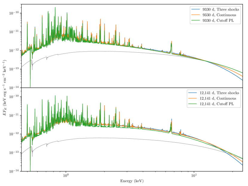
Figure 10: Three different models fitted to the first (upper panel) and last (lower panel) NuSTAR epochs. The models are the standard three thermal shocks model (blue), the continuous temperature model (orange), and two thermal shocks with an additional cutoff PL (green). We also show the cutoff PL component separately (thin gray lines). The blue line in the upper panel (largely covered by the other lines) shows the same model as in Figure 6, but we note that the $y$-axes are different to better follow conventions.

We find no indications of a non-thermal contribution to the X-ray spectrum. The thermal models describe the data well and neither replacing the hottest plasma component with a cutoff PL, nor adding an additional PL component, results in a better model. Below, we motivate this conclusion in more detail.

First, we use the standard three-shock model, but replace the hottest shock component with a cutoff PL. This phenomenological cutoff PL can be interpreted as a hot 10–20 keV free-free component, synchrotron emission, or potentially represent a PWN. The photon index of the cutoff PL is frozen to $\Gamma=2$ to prevent degeneracies with the shock components. This value for $\Gamma$ is similar to that of the Crab Nebula (Bühler & Blandford, 2014). We verify that choosing $\Gamma=1.5$ or $2.5$ does not significantly affect the conclusions.

Freezing the photon index effectively forces the cutoff PL to dominate at higher energies. The cutoff energies and normalizations are left free and fitted to all NuSTAR epochs. This fit focuses on higher energies and, therefore, we omit the RGS data and instead freeze the coolest shock component. All non-thermal components are harder than the average shape of the thermal spectra. This implies that any non-thermal contribution is increasingly subdominant toward lower energies (e.g. Figures 6 and 10). Thus, the RGS data will not affect the hard non-thermal components.

Importantly, the Fe abundance needs to be free in these fits, but still constant across different epochs. This is necessary because the Fe abundance was fitted using the three-shock model (Section 3.2), where the hottest component captured the Fe K line complex. With the hottest component replaced, the Fe abundance will naturally need to increase. This is because the cutoff PL dominates at those energies and the line strength is proportional to the abundance.

We show a comparison of the three-shock model, continuous temperature model, and two-shock plus cutoff PL model in Figure 10. From the fits of the cutoff PL model, we obtain an average fitted cutoff energy of 8 keV and an Fe abundance of $2.0_{-0.5}^{+1.0}$ relative to the LMC Fe abundance. For reference, the corresponding Fe abundances are $1.8_{-0.6}^{+1.1}$ for $\Gamma=1.5$ and $2.5_{-0.8}^{+2.0}$ for $\Gamma=2.5$. Statistically, the goodness with the $\Gamma=2$ cutoff PL is $\chi^{2}=2594$ for 2778 DoF, compared to $\chi^{2}=2597$ for 2771 DoF for the three-shock model. However, we consider the Fe abundance to be unreasonably high (further discussed in Section 5.3) and a strong indication that the thermal contribution around 6.5 keV is underestimated using this model. Furthermore, the fits to different epochs result in cutoff energies ranging from 2.4–13 keV and normalizations spanning a factor of 3. This is compensated by changes of the best-fit temperature of the warmer of the two shocks from 1.5–5.4 keV. These factors all indicate that it is possible to include a non-thermal component, but it is not statistically nor physically motivated, and adds unnecessary complexity to the model. We note that we consider adding a cutoff PL as introducing additional complexity since it is composed of a qualitatively new component even though, formally, the number of DoF is reduced from 2778 to 2771. Therefore, we reject the model with the cutoff PL.

Another possibility is to simply add a non-thermal component to the three-shock model. In this case, a cutoff energy cannot be constrained, so we add a PL with $\Gamma=2$. We note that the Fe abundance remains frozen to our adopted standard value of 0.62 of LMC since the hottest shock component still dominates around 6.5 keV. Fitting yields an improvement of $\Delta\chi^{2}=-2.71$ for 1 additional DoF (2770 DoF in total) compared to the standard three-shock model. This means that the PL results in a negligible improvement and it is not motivated to include it.

To put a limit on the non-thermal emission, we start from the fit above with the additional PL component with $\Gamma=2$. By fitting simultaneously to all observations, we obtain one average upper limit instead of an upper limit at each epoch. The upper limit is computed by finding the PL normalization that results in an increase of $\Delta\chi^{2}=7.740$ relative to the best fit (using the XSPEC task error). We take the flux of the PL component with this new normalization as a 3$\sigma{}$ upper limit. The resulting limits are $7\times{}10^{-14}$  erg s^-1 cm^-2 between 3–8 keV and coincidentally also $7\times{}10^{-14}$  erg s^-1 cm^-2 between 10–24 keV.

These limits are clearly model-dependent, as further discussed in Section 5.3. A very conservative, model-independent limit is to consider the total fluxes as upper limits (Table 5), with the 10–24 keV range likely being the most relevant.

4.6 35–65 keV Limit on the Compact Object

We obtain a 3$\sigma{}$ upper limit on any flux from SN 1987A in the 35–65 keV range of $8\times{}10^{-14}$ erg s^-1 cm^-2. This was computed using a $\Gamma=2$ PL component without an underlying thermal component. This limit does not require model assumptions because SN 1987A is not detected in this energy range, which is above the continuum emission from the ER and below the radioactive ⁴⁴Ti line emission. This limit is primarily relevant for the compact object but, naturally, also applies to any other emission component.

4.7 Radioactive ${}^{44}Ti$ Line Emission

The ⁴⁴Ti decay chain produces high-energy X-ray lines, which have been detected by NuSTAR (see Boggs et al. 2015 for details). The radioactive K$\alpha$ lines in the XMM-Newton energy range are studied separately in Appendix B. We repeat the analysis of Boggs et al. (2015), but with the inclusion of our new data.

Following the baseline case of Boggs et al. (2015), we tie the fluxes, energies, and widths of the two lines. This can be done because the relative fluxes ($96.4/93.0$) and energies ($78.32\text{~{}keV}/67.87$ keV) are given by the relative yields and transition energies, respectively. The widths are simply proportional to the energy. This implies that both lines are fitted simultaneously, using the free parameters of only one line. We choose to report the fitted parameters for the 67.87 keV line below.

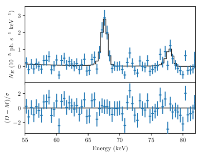
Figure 11: Fits of the ⁴⁴Ti lines. The panels are structured as in Figure 8. The large difference between the two lines are due to the highly varying instrumental response within this energy range, which is close to the upper energy limit of NuSTAR. For visual clarity, the data shown are the rebinned sum of all NuSTAR observations.

We show the fitted ⁴⁴Ti lines in Figure 11. The best-fit energy of the 67.87 keV line is $67.64^{+0.12}_{-0.09}$ keV, compared to $67.64^{+0.09}_{-0.09}$ keV of Boggs et al. (2015). We note that separate fits to the individual modules yield $67.70^{+0.17}_{-0.13}$ keV for FPMA and $67.61^{+0.13}_{-0.14}$ keV for FPMB. In terms of velocities, our redshifts (after correcting for recession velocity and the look-back effect; Boggs et al. 2015) are $670^{+520}_{-380}$ km s^-1 for the simultaneous fit to both modules, $420^{+740}_{-560}$ km s^-1 for FPMA, and $820^{+580}_{-640}$ km s^-1 for FPMB.

The difference between the modules indicates that systematic uncertainties could be comparable to the statistical uncertainties. In this context, systematic uncertainties include all factors related to the data reduction and analysis, in addition to the instrumental calibration uncertainty (see also Appendix C). For reference, the reported energy calibration uncertainty at 67.87 keV is 0.06 keV (Madsen et al., 2015), corresponding to 270 km s^-1.

Analogous to the redshift, we provide ⁴⁴Ti mass estimates based on both the joint fit and fits to the individual modules. The combined analysis yields a 67.87 keV line flux of $3.7_{-0.6}^{+0.6}\times{}10^{-6}$ photons s^-1 cm^-2, which corresponds to an initial ⁴⁴Ti mass of $1.73_{-0.29}^{+0.27}\times{}10^{-4}$ M_☉. When converting ⁴⁴Ti fluxes to masses, we use a distance of 51.2 kpc and correct the observed fluxes by 3 % to account for Compton scattering by the ejecta (Alp et al. 2018a and Section 5.5 below).

Our mass estimate is comparable to the value $1.5_{-0.3}^{+0.3}\times{}10^{-4}$ M_☉ reported by Boggs et al. (2015), and $1.5_{-0.5}^{+0.5}\times{}10^{-4}$ M_☉ obtained from modeling of an optical spectrum by Jerkstrand et al. (2011). Furthermore, a slight difference is apparent between FPMA and FPMB also for the inferred masses. The FPMA estimate is $1.86_{-0.40}^{+0.43}\times{}10^{-4}$ M_☉, compared with $1.57_{-0.38}^{+0.43}\times{}10^{-4}$ M_☉ obtained from FPMB. This further highlights the subtle systematic uncertainties, which are important to consider.

5 Discussion

5.1 Physical Interpretation of the Thermal Emission

Thermal shock models adequately describe the observed X-ray spectra. We find no indications of a non-thermal component in the spectrum. Instead, we favor an interpretation where the low- and mid-temperature components originate from the ER clumps, while the high-temperature component is produced in low-density regions. The ER clumps could give rise to a range of temperatures as a result of varying incident shock angles, hydrodynamic disruption of the clumps, and a mix of radiative and adiabatic shocks of varying temperatures. The low-density regions refer to both the diffuse gas between the ER clumps and the high-latitude H ii region. This interpretation is motivated by a number of independent simulations and observations across the electromagnetic spectrum. We present these points separately for the ER clumps in Section 5.1.1 and low-density regions in Section 5.1.2, before tying things together in Section 5.1.3.

5.1.1 Emission from the ER Clumps

Previous studies of the ER clumps have shown the following.

• Optical and ultraviolet (UV) observations resolve the hotspots in the ER and show slow, radiative shocks with velocities up to ${\sim}700$  km s^-1 into clumps with pre-shock densities of up to $6\times{}10^{4}$ cm^-3 (Pun et al., 2002; Gröningsson et al., 2008; Larsson et al., 2019).

• There is a clear east-west asymmetry in the X-ray emission (Frank et al., 2016; Cendes et al., 2018). The X-ray emission below 2 keV is stronger to the west and follows the optical ER emission. This implies that the ER clumps dominate the $<2$ keV X-ray flux.

• The inferred ER radii in optical and X-rays also indicate that the $<2$ keV X-rays originate from the same region as the optical ER (Frank et al., 2016; Larsson et al., 2019). Furthermore, the $<2$ keV radius appears to separate into two components after 6000 d when divided at 0.8 keV, with the $<0.8$ keV component expanding the slowest.

• Simulations of shock interactions with the ER clumps reveal a complex picture (Borkowski et al., 1997; Pun et al., 2002; Orlando et al., 2015, 2019). The interactions clearly disrupt the clumps, disperse the clump material, and produce both radiative and adiabatic shocks of varying temperatures. The temperatures are expected to range from ${\sim}$0.2 to 1 keV depending on the shock velocities, densities, and incidence angle.

In this paper, we have presented new light curves of the soft X-ray emission (Figure 4). These are in line with previous conclusions and further corroborate the hypothesis that the soft X-ray emission is primarily produced in the ER clumps. Figure 4 shows that X-rays below 2 keV have a similar evolution as optical and there are indications that the 0.45–0.7 keV light curve is more strongly correlated with the optical emission than the 0.5–2 keV emission after 10,000 d. This may be explained as a result of the cooling time ($t_{\mathrm{cool}}$) depending on the shock velocity ($V_{\mathrm{s}}$) and density ($n$) as

$$t_{\mathrm{cool}}=47\left(\frac{V_{\mathrm{s}}}{500\text{~{}km~{}s${}^{-1}$}}\right)^{3.4}\left(\frac{n}{10^{4}\text{~{}cm}^{-3}}\right)^{-1}\text{~{}yr}$$ (3)

(Gröningsson et al., 2008). Densities much higher than $10^{4}$ cm^-3 are therefore required to produce optical emission for shocks faster than $500$ km s^-1. Consequently, a decreasing fraction of the X-rays above ${\sim}$2 keV is expected to follow the optical emission.

5.1.2 Emission from the Low-density Regions

In addition to studies indicating that the X-ray emission below 2 keV originates from the ER clumps, the X-rays above 2 keV likely originate from a region of wider latitudinal extent and lower density. This is primarily motivated by the following arguments.

• Already in 1997, HST observations revealed Ly$\alpha$ and H$\alpha$ emission extending to $\pm$30° above and below the ER (Michael et al., 1998). Later, radio and X-ray observations showed similar latitudinal extents (Ng et al., 2009, 2013; Cendes et al., 2018). This is also consistent with VLT observations, which show H$\alpha$ emission extending to velocities higher than ${\sim}$13,000  km s^-1 in 2012 (Fransson et al., 2013). Later VLT observations continue to show similar velocities (Larsson et al., 2019).

• In contrast to the $<2$ keV X-rays, the asymmetries of the $>2$ keV X-rays follows the radio torus and are brighter to the east. The new optical emission beyond the ER is also stronger to the east, indicating stronger interaction at high latitudes in this direction (Larsson et al., 2019).

• The inferred ER radii in radio and X-rays indicate that the $>2$ keV X-ray and radio emission is produced by shocks with velocities of ${\sim}$3000  km s^-1 (Frank et al., 2016; Cendes et al., 2018). We note that small discrepancies between the X-ray and radio radii could be due to a combination of limited spatial resolution, projection effects, and overlap between different components (energies) in X-rays.

• X-ray emission from the fastest shocks moving in the low-density regions are expected to produce a faint, broad component in the line profiles. This could potentially reveal the relative contributions of different shock velocities to the X-ray emission below 2 keV. A 20 % contribution from a broad component corresponding to a velocity of ${\sim}$9000  km s^-1 has been reported by Dewey et al. (2012), but the limited energy resolution and line blending complicate analyses. The X-ray line profiles have also been successfully fitted without a broad component (Zhekov et al., 2009). We do not investigate the line profiles in detail, but obtain good fits using models without an additional broad component. However, optical and UV lines show directly that a ${\sim}$13,000 km s^-1 component is present (Michael et al., 1998; Fransson et al., 2013). For these very fast shocks, the slow equipartition between the electrons and ions likely leads to a considerably lower electron than ion temperature, which we discuss below.

We present the 3–8 and 10–24 keV light curves to 2020 in Figure 4. The 3–8 keV X-ray light curve follows the radio light curve relatively well. The 10–24 keV light curve has a flatter evolution, but this is likely the effect of a slight decrease in temperature (Figure 7), rather than an indication of a different physical origin (Section 5.3). This shows that the X-ray light curves agree with the picture painted by the previous, independent observations.

5.1.3 The Combined Picture

The points above, along with further pieces of information, form a combined picture. Assuming equipartition between electrons and protons behind the shocks, the temperature is related to the shock velocities by

$$k_{\mathrm{B}}T=1.4\left(\frac{V_{\mathrm{s}}}{1000\text{~{}km~{}s${}^{-1}${}}}\right)^{2}\text{~{}keV}$$ (4)

for our adopted abundances. Using observed velocities in the optical and X-rays one can therefore relate these to the observed temperatures we find.

The optical ER expands with a velocity of $680\pm{}50$ km s^-1 (Larsson et al., 2019) since ${\sim}$7700 d, and line profiles of the optical hotspots show velocities up to 700–1000 km s^-1, depending on the geometry, with a FWHM of ${\sim}300$ km s^-1 (Fransson et al., 2015). This corresponds to a shock temperature of $k_{\mathrm{B}}T=0.1$–1 keV. Therefore, these shocks may be at least partially responsible for the two lower temperature components. These shocks will be radiative for densities up to ${\sim}6\times 10^{4}$ cm^-3.

From the Chandra X-ray observations later than 6000 d, Frank et al. (2016) find an expansion velocity of $1851\pm 105$  km s^-1 for the 0.5–2 keV band and $3071\pm 299$ km s^-1 for the 2–10 keV band. Assuming equipartition, the former corresponds to $k_{\mathrm{B}}T=4.8$ keV, while the latter corresponds to 13.2 keV. To reconcile the high velocity in the 0.5–2 keV band with the temperature one needs to assume that the emission in the 0.5–2 keV band has contributions from both slower radiative shocks, also emitting in the optical, and faster, adiabatic shocks emitting mainly in X-rays. Deviations from equipartition could also be contributing. This is primarily relevant for the hottest component and is described in more detail below. We note that Frank et al. (2016) find an expansion velocity of $-110\pm{}313$ km s^-1 in the 0.3–0.8 keV range after 6000 d. This shows that the inferred velocities within X-ray energy ranges are combinations from shocks of varying expansion velocities.

Finally, to connect the higher velocities seen by Frank et al. (2016) in the 2–10 keV band to the 4 keV component that we find, one has to assume only partial equipartition of the ion and electron temperatures behind these faster shocks. Slow equilibration behind fast shocks has been inferred from supernova remnants, where a ratio of electron to ion temperature of $T_{\mathrm{e}}/T_{\mathrm{p}}\propto 1/V_{\mathrm{s}}^{2}$ has been proposed for Balmer dominated shocks into neutral media (Ghavamian et al., 2013). In the context of SN 1987A, France et al. (2011) find $T_{\mathrm{e}}/T_{\mathrm{p}}\approx 0.14$–0.35 from observations of the reverse shock with a velocity of ${\sim}$10,000 km s^-1. X-ray emission from the reverse shock, with an electron temperature of 20–49 keV (assuming $T_{\mathrm{e}}/T_{\mathrm{p}}$ in the range above), is presumably too faint to be seen, because of the low ejecta and CSM densities.

In addition to the temperatures, the densities inferred from the fitted parametrized ionization age (Section 4.4) are comparable to previous estimates. Based on optical data, the densities of the unshocked ER clumps are estimated to reach $6\times{}10^{4}$ cm^-3 (Pun et al., 2002; Gröningsson et al., 2008). Furthermore, modeling based on radio and optical data find densities of $10^{3}$ cm^-3 in the diffuse ER (Mattila et al., 2010) and a density of $10^{2}$ cm^-3 in the surrounding H ii region (Chevalier & Dwarkadas, 1995; Lundqvist, 1999). Our estimates are uncertain, but capture the trend of a decreasing ionization age as a function of increasing energy. This is an indication that cooler, slower shocks originate from regions of higher density.

There are a number of observables that are not completely explained by our model. We are unable to provide a natural reason for why the temperature distribution produced by the clumps would be bimodal. It could simply be that the apparent bimodality is a smoother broad distribution in reality. Furthermore, we assume that the hottest component arises from regions spanning a wide range of densities. Thus, it is somewhat surprising that the temperature distribution shows such a narrow peak around 4 keV. A possibility is that the relatively homogeneous H ii region dominates this component.

However, given the complexity of the system, we believe that these are minor issues. There are also significant modeling uncertainties underlying the shock model used for the analysis, especially at temperatures below ${\sim}$1 keV where radiative losses become important (Section 3.1). In addition, other emission components, such as the reverse shock propagating back into the ejecta, are predicted to contribute at some level at current epochs (Orlando et al., 2015, 2019). This is likely an underlying component, which is absorbed into our three-component interpretation.

The spectra from different epochs are relatively similar except for a decrease in temperature of the hottest component in the last epoch (Figure 7). The geometry is too complex for detailed predictions of the temporal evolution. We simply note that a slight decrease in temperature is physically reasonable based on a general deceleration of the ejecta and the blast wave. Therefore, a completely thermal interpretation of the spectrum is consistent with the observed temporal evolution.

To summarize, the combination of all available information implies that the X-ray emission likely is of purely thermal origin. This emission would be produced by shocks with typical temperatures of 0.3–0.9 keV in the ER clumps, and 4 keV in the surrounding diffuse ER and H ii region. However, we conclude by cautioning not to overinterpret the data. This is simply our favored simplification of a clearly more complex reality.

5.2 Previous Thermal Modeling

Table 6: Comparison with Previously Fitted Thermal Model Temperatures

Date	Epoch	Model	Energy range	$k_{\mathrm{B}}T_{1}$	$k_{\mathrm{B}}T_{2}$	$k_{\mathrm{B}}T_{3}$	Reference
(YYYY-mm-dd)	(d)		(keV)	(keV)	(keV)	(keV)
2019-11-27	11,965	Two shocks	0.3–10	0.6	$\cdots$	2.5	Sun et al. (2021)
2018-09-15	11,527	Two shocks	0.5–3	0.5	$\cdots$	1.5	Bray et al. (2020)
2017-10-15	11,192	Two shocks	0.3–10	0.6	$\cdots$	2.3	Sun et al. (2021)
2016-11-02	10,845	Two shocks	0.3–10	0.7	$\cdots$	2.5	Sun et al. (2021)
2015-09-17	10,433	Two shocks	0.5–8	0.3	$\cdots$	2.1	Frank et al. (2016)
2014-09-18	10,069	Two shocks	0.5–3	0.5	$\cdots$	1.4	Bray et al. (2020)
2014-07-11	${\sim}$10,000	Three shocks	0.45–24	0.5	1	4	This paper
2014-07-11	${\sim}$10,000	Continuous	0.45–24	0.3	0.9	4.2	This paper
2011-03-03	8774	Three shocks	0.6–5	0.5	1.2	2.7	Dewey et al. (2012)
2009-01-30	8012	Two shocks	0.4–8	0.5	$\cdots$	2.4	Sturm et al. (2010)
2007-09-10	7504	Two shocks	0.4–7	0.5	$\cdots$	1.9	Zhekov et al. (2009)
2007-09-10	7504	Continuous	0.4–7	0.5	$\cdots$	2.2	Zhekov et al. (2009)
2007-03-25	7335	Three shocks	0.6–5	0.5	1.2	4.3	Dewey et al. (2012)
2007-01-20	7271	Three shocks	0.3–8	0.3	1.7	2.7	Zhekov et al. (2010)
2007-01-17	7268	Two shocks	0.2–10	0.4	$\cdots$	3.0	Heng et al. (2008)
2005-07-14	6716	Two shocks	0.3–8	0.3	$\cdots$	2.3	Park et al. (2006)
2004-08-30	6398	Two shocks	0.4–7	0.5	$\cdots$	2.7	Zhekov et al. (2006)
2004-08-30	6398	Continuous	0.4–7	0.5	$\cdots$	3	Zhekov et al. (2006)
2003-05-10	5920	Two shocks	0.2–9	0.3	$\cdots$	3.1	Haberl et al. (2006)
2000-12-07	5036	Two shocks	0.3–8	0.2	$\cdots$	3.2	Park et al. (2006)
2000-12-07	5036	Three shocks	0.3–8	0.2	2.9	5.1	Zhekov et al. (2010)
2000-12-07	5036	Three shocks	0.4–8.1	0.7	1.2	4.2	Dewey et al. (2012)
2000-01-20	4714	Two shocks	0.3–9	0.2	$\cdots$	2.0	Haberl et al. (2006)

Our spectral analysis indicates the presence of three components. Only a few previous analyses have used three shock components (Zhekov et al., 2010; Dewey et al., 2012; Maggi et al., 2012). In contrast, most earlier studies found bimodal temperature distributions (Zhekov et al., 2006, 2009; Dewey et al., 2008) or used two shock components (Haberl et al., 2006; Heng et al., 2008; Sturm et al., 2010; Park et al., 2011; Helder et al., 2013; Frank et al., 2016; Bray et al., 2020).

We provide a comparison of our fitted temperatures with a selection of literature values in Table 6. Our fits find higher maximum temperatures than most other analyses, especially at comparable epochs. Notably, even the previous analyses with continuous temperature models only found two peaks. The differences are primarily due to the wider energy range provided by NuSTAR, which we show in Appendix D (Table 9).

Some previous fits found comparable maximum temperatures at epochs earlier than ${\sim}7000$ d, before the ER interaction peak. This is likely because the continuum from the surrounding low-density region was dominant even below ${\sim}$5 keV, which is the range where other analyses are primarily sensitive. In addition to the values in Table 6, Maggi et al. (2012) mention that the hottest temperature is $>3.5$ keV in XMM-Newton observations from 7000–9000 d, but they did not present a complete spectral analysis. There appears to be a trend that XMM-Newton data result in higher temperatures than Chandra data, likely due to the higher high-energy sensitivity of XMM-Newton. This strengthens the argument that NuSTAR data is required to more robustly fit shock components with temperatures above ${\sim}$3 keV (see Appendix D for further details).

5.3 Non-Thermal Emission

Even though we favor a thermal interpretation of the X-ray emission, it remains possible that there is a non-thermal contribution. In Section 4.5, we showed that a model where the hottest shock component is replaced by a cutoff PL provides a fit of comparable quality as the purely thermal model. However, an important feature for the interpretation of the X-ray spectrum is the Fe K line complex around 6.4–6.9 keV (Figure 8).

The presence of a clear Fe K line in the observed X-ray spectrum implies that at least part of the hard X-ray emission is of thermal origin. The strength of the line predicted by the thermal model is proportional to the fitted Fe abundance. Therefore, in principle, it is possible to accommodate an additional non-thermal component by increasing the Fe abundances. This results in a higher modeled thermal line-to-continuum ratio, which would then need an additional non-thermal continuum component to properly match the observed line-to-continuum ratio. Consequently, the Fe abundance would be artificially suppressed if we attempt to fit a purely thermal model to a spectrum that has a significant fraction of non-thermal emission.

We find that our best-fit Fe abundance of 0.62 relative to the LMC (Table 3.2) provides adequate fits to the Fe K line (Figure 8; see also Sturm et al. 2010; Maggi et al. 2012). We consider an Fe abundance of $0.62^{+0.02}_{-0.01}$ relative to the LMC to be reasonable and, hence, not an indication of an underlying non-thermal component. This is further strengthened by the independent Fe estimate of $0.56^{+0.31}_{-0.31}$ relative to the LMC based on optical spectroscopy (Mattila et al., 2010). If there is a significant non-thermal contribution, we expect a substantially lower fitted Fe abundance.

The correlation between the 3–8 keV and radio light curves (Figure 4) could be interpreted as a suggestion that (part of) the hard X-rays are non-thermal. However, the 10–24 keV light curve rises much more slowly than the 3–8 keV light curve. This is opposite to what would naively be expected if the hard X-rays are of non-thermal origin. The 10–24 keV flux would be expected to increase faster because thermal X-rays would contribute more to the 3–8 keV than the 10–24 keV range in relative terms. In this scenario, it is implicitly assumed that the thermal flux would not increase as fast as the radio flux, based on comparisons between radio and soft X-rays. Since the 10–24 keV flux increases more slowly than 3–8 keV, a non-thermal model would need to have a contrived spectral evolution, which we disfavor against a simple, slight decrease in maximum temperature in a completely thermal model.

Following the above arguments, we conclude that the evidence for a non-thermal component is weak. Instead, we use the data to compute upper limits (Sections 4.5 and 4.6) as constraints on a non-thermal component. These limits constrain cosmic ray acceleration and the properties of the compact object, as discussed below.

5.4 Cosmic Ray Acceleration

The shocks from the CSM interactions around SN 1987A are expected to accelerate relativistic particles (Berezhko et al., 2011, 2015; Dwarkadas, 2013). The relativistic electrons from this acceleration process are thought to produce the observed radio emission and it is possible that the same non-thermal synchrotron component extends to X-ray energies. From a theoretical perspective, Berezhko et al. (2015) present a prediction for the non-thermal X-ray contribution associated with cosmic ray acceleration. Using their model for cosmic ray acceleration (Berezhko & Ksenofontov, 2000, 2006), they find a peak 35–65 keV flux of $5\times{}10^{-14}$ erg s^-1 cm^-2 at 9280 d (Figure 6), which is marginally consistent with our upper limit of $8\times{}10^{-14}$  erg s^-1 cm^-2. However, the predicted fluxes at 3–8 ($1.4\times{}10^{-13}$ erg s^-1 cm^-2) and 10–24 keV ($1.2\times{}10^{-13}$ erg s^-1 cm^-2) exceed the corresponding model-dependent limits by a factor of ${\sim}$2 (Section 4.5).

Recently, it has been reported that a brightening GeV source has been detected by Fermi/LAT, possibly associated with SN 1987A (Malyshev et al., 2019; Petruk et al., 2019). The GeV emission could be of either hadronic or leptonic origin. In the hadronic scenario, accelerated protons interact with protons in the ISM and produce neutral pions, which decay into gamma rays. On the other hand, a leptonic origin implies relativistic bremsstrahlung and inverse Compton scattering by accelerated electrons. The scenario that most directly affects the observed X-ray emission is if the GeV emission is leptonic and a significant part of the X-ray emission is non-thermal. In this case, a steep rise in the GeV emission would be correlated with a more rapid increase in the (hard) X-ray light curve due to an increasing non-thermal component.

The observed GeV light curve increases by at least a factor of 2 between 2012 and 2018 (Malyshev et al., 2019; Petruk et al., 2019). This time range roughly coincides with the first and last NuSTAR observation. Both the X-ray and radio light curves continue to smoothly increase at steady rates by factors of ${\sim}$1.5 over this time interval (Figure 4). Notably, the high-energy X-ray component above 10 keV is the flattest and barely increases during this time. Therefore, we conclude that there is no obvious correlation between any part of the X-ray or radio light curve with the GeV increase. This indicates that the GeV emission is of hadronic origin or unrelated to SN 1987A.

5.5 Limits on the Compact Object

The upper limit on a non-thermal component in the NuSTAR data places new constraints on the compact object at hard X-ray energies and complements the multi-wavelength limits presented in Alp et al. (2018b). Currently, the only tentative indication of a neutron star is the bright spot observed in a 679 GHz ALMA image (Cigan et al., 2019). This could potentially be the result of local dust heating by thermal emission from a neutron star, as suggested in Alp et al. (2018b). A PWN can also match the observation, but this model is practically unconstrained and can fit almost any data. Therefore, we find no reason to favor the PWN model over passive thermal neutron star heating. However, we stress that the conclusions from the ALMA image are uncertain due to a low S/B, possible structure in the underlying dust emission, and poorly constrained spectrum and luminosity of the possible source. More data are needed to clarify the nature of the ALMA hotspot.

Recently, Greco et al. (2021) interpreted the 2012–2014 NuSTAR data as indications of a PWN and rejected a purely thermal interpretation of the data. This is in stark contrast to our results. As we show in Section 4.5, we are unable to motivate a model with a non-thermal component.

We also search for pulsed emission between 10 and 20 keV (Appendix A), which could be present if a PWN is contributing. No pulsations are detected and the pulsed fraction is constrained to less than $15$ % of the total source flux between 10–20 keV.

Adding a PWN component to a thermal model will, of course, still fit the data, but the additional complexity cannot be statistically nor physically motivated. Furthermore, even if the adopted model contains a non-thermal component, we believe that more likely explanations are synchrotron emission from shock accelerated electrons (Berezhko et al., 2011, 2015; Dwarkadas, 2013) or the high-energy tail of a free-free component. As outlined in Section 5.1.3, the reverse shock is expected to produce a faint component with $k_{\mathrm{B}}T=20$–49 keV. Both shock synchrotron and free-free components are expected, and are likely to be present at low levels compared to the dominant thermal emission.

Finally, any proposed model for the compact object in SN 1987A must form a coherent physical picture with observations at other wavelengths and the total energy budget of the system. Due to the excellent observational coverage, the allowed bolometric luminosity of the neutron star is constrained to be lower than 10–100 L_☉ (Alp et al., 2018b). The quoted luminosity interval accounts for the uncertainty in the amount of newly formed dust in the ejecta along the line of sight.

Our 35–65 keV flux limit provides the deepest constraints on any X-ray emission from a compact object in SN 1987A. X-ray emission from the compact object is affected by absorption since it resides close to the center of the ejecta (Alp et al., 2018a). The high metallicity of the SN ejecta results in photoabsorption dominating up to ${\sim}$30 keV. This implies that the cross section above 30 keV is dominated by Compton scattering, and that the opacity at these energies is many order of magnitudes lower than in the 0.3–10 keV band. We estimate the 35–65 keV absorption using a three-dimensional neutrino-driven SN explosion model (Alp et al., 2018a), specifically the B15 model from Wongwathanarat et al. (2015). This is the same absorption model as was used for SN 1987A by Alp et al. (2018b). We find that approximately 5 % of the 35–65 keV flux is expected to be absorbed at 10,000 d, which we henceforth correct for. For reference, the optical depth to center of the ejecta at current epochs is ${\sim}100$ at 1 keV, ${\sim}$3 at 5 keV, and ${\sim}$0.03 at 50 keV (Alp et al., 2018a).

The absorption-corrected 35–65 keV limit is $8\times{}10^{-14}$ erg s^-1 cm^-2 (Section 4.6) and corresponds to approximately $2\times{}10^{34}$ erg s^-1 (7 L_☉) for a distance of 51.2 kpc. This is equivalent to a fraction of ${\sim}$0.05 of the Crab Pulsar (excluding the Nebula; Bühler & Blandford 2014) and is the most constraining direct limit on a Crab Pulsar-like spectrum. This is deeper than previous hard X-ray limits, but does not qualitatively affect any conclusions in Alp et al. (2018b).

6 Summary and Conclusions

We have studied new NuSTAR observations of SN 1987A obtained in 2020, and performed a combined analysis with archival NuSTAR data from 2012 to 2014 and XMM-Newton data from 2000 to 2019. This combination covers a wide X-ray interval ranging from 0.45 to 78 keV. In conjunction with the long temporal baseline, it provides a unique X-ray view of the complex SN 1987A system.

The X-ray light curves in different energy bands have evolved significantly over the past few epochs. The 10–24 keV flux remained practically constant between 9300 and 12,000 d (2012–2020). In contrast, the 3–8 keV flux was rising, but has tentatively started to flatten after 11,000 d (2017). Previously published radio light curves only extend to 10,942 d (2017; Cendes et al. 2018), but followed the rising phase of the 3–8 keV emission up to that point. The 0.5–2 keV emission has clearly decreased since 10,000 d (2015). In particular, we find that the correlation between optical and X-rays is increasingly strong for decreasing X-ray energies.

We favor a purely thermal description of the X-ray spectra. Acceptable fits require three shocked plasma components at temperatures of approximately 0.3, 0.9, and 4 keV. We obtain very similar results using a model with a continuous temperature distribution. Previous studies have mostly used two components with temperatures of approximately 0.5 and 2.5 keV. The difference is most likely due to the extended energy range offered by NuSTAR, which has not been used for fits of purely thermal spectra in previous studies.

Our favored interpretation associates the 0.3 and 0.9 keV components with the dense ER clumps, whereas the 4 keV emission originates from the diffuse ER gas and the high-latitude H ii region. There is no obvious explanation for why the ER clumps would produce emission at two distinct temperatures. The bimodality between the 0.3 and 0.9 keV components is, however, uncertain and could be the manifestation of a smoother broad distribution.

We find no evidence for a non-thermal contribution to the X-ray data, neither from the temporal nor spectral analysis. The 10–24 keV flux does not follow the synchrotron radio light curve, which would be the most natural expectation if the X-ray emission is increasingly dominated by synchrotron emission from shock-accelerated electrons at higher energies. The spectral fits do not improve when a PL is added, and the clear Fe K line complex is also well captured by a purely thermal model. Replacing the hottest thermal component with a non-thermal component results in a statistically acceptable fit, but requires an unreasonably high Fe abundance. Furthermore, the thermal interpretation forms a consistent picture with temporal, spectral, and spatial multi-wavelength information from the literature. However, we note that this does not firmly exclude a, possibly weak, non-thermal contribution.

A brightening of SN 1987A at GeV energies has recently been reported (Malyshev et al., 2019; Petruk et al., 2019). We find no clear correlation between the GeV and X-ray emission. This indicates that the GeV emission is dominated by hadronic processes or unrelated to SN 1987A. However, in the leptonic scenario, predictions for the level of X-ray emission and the high-energy synchrotron cooling cutoff are both uncertain. This leaves the leptonic channel possible, but requires it to be consistent with the observational upper limits ($7\times{}10^{-14}$ erg s^-1 cm^-2 from 10 to 24 keV and $8\times{}10^{-14}$ erg s^-1 cm^-2 from 35 to 65 keV).

We also analyze the radioactive ⁴⁴Ti lines using all the NuSTAR data to repeat the analysis first performed by Boggs et al. (2015). We find a redshift of $670^{+520}_{-380}$ km s^-1 and an initial mass of $1.73_{-0.29}^{+0.27}\times{}10^{-4}$ M_☉. However, there appear to be potentially significant systematic uncertainties, indicated by differences in the results from different analysis methods. These uncertainties are of approximately the same magnitude as the statistical uncertainties in both the redshift and mass, which should be considered in subsequent analyses and interpretations.

XMM-Newton observations constrain the radioactive K$\alpha{}$ lines from $\text{${}^{55}$Fe{}}\rightarrow{}\text{${}^{55}$Mn{}}$ and $\text{${}^{44}$Ti{}}\rightarrow{}\text{${}^{44}$Sc{}}$ (Appendix B). No lines are firmly detected, but the initial ⁵⁵Fe mass is inferred to be $<4.2\times{}10^{-4}$ M_☉, whereas the $1.7\times{}10^{-4}$ M_☉ ⁴⁴Ti mass from NuSTAR is consistent with a non-detection at 4.1 keV in XMM-Newton. Nucleosynthesis simulations predict ⁵⁵Fe masses in the range 1–20$\times{}10^{-4}$ M_☉ (Leising, 2006; Popov et al., 2014; Sieverding et al., 2020). Our results favor a ⁵⁵Fe mass toward the lower end of this range. However, this relies on the 10HMM model. The masses from simulations are also based on a diversity of SN progenitors and the progenitors are exploded using different methods.

Since we favor a purely thermal model for the full X-ray spectrum, we argue that there are no indications of a pulsar. Even if a faint non-thermal component is present, it is more likely to be shock accelerated synchrotron emission or the high-energy tail of a free-free component. We also constrain the pulsed fraction of the 10–20 keV flux to be less than $15$ % (Appendix A).

The NuSTAR data constrain the 35–65 keV luminosity of the compact object in SN 1987A to be lower than $2\times{}10^{34}$ erg s^-1 (7 L_☉; $8\times{}10^{-14}$ erg s^-1 cm^-2). We put this into context by comparing the limit with previous multi-wavelength observations. These show that the bolometric luminosity of the compact object must be lower than 10–100 L_☉ (range due to uncertain properties of the dust). Currently, an ALMA image at 679 GHz is the only tentative hint of a neutron star in SN 1987A, which needs to be verified with higher quality data.

Our analysis shows that NuSTAR observations are required for a complete X-ray view of SN 1987A. NuSTAR is the only instrument sensitive enough to detect the X-ray continuum above 10 keV, which affects the interpretation of the entire X-ray spectrum. The optical depth to the compact object is currently ${\sim}$1 at 10 keV, which implies that practically no X-rays of lower energy escape, unless clumping is stronger than simulations indicate. This means that NuSTAR could be the most sensitive telescope to search for X-ray emission from a potential neutron star. If the GeV emission keeps increasing, it is also possible that a non-thermal component will emerge in the NuSTAR range. Future NuSTAR observations of SN 1987A are therefore critical to complement the regular monitoring at other wavelengths.

Appendix A Search for Pulsed Emission

We search for pulsed X-ray emission from SN 1987A since this would be the smoking gun of a pulsar. For this timing analysis, we use the observations from 2012 to 2014 (all NuSTAR epochs except for the last). Restricting the temporal baseline to two years improves the sensitivity. A number of factors contribute to this. First, a shorter temporal baseline requires a lower resolution in rotational period since period errors propagate proportionally to the baseline. Second, a lower resolution in pulsar spin-down rate is required since this also propagates into the phase solution. Furthermore, limiting the time range to two years reduces the risk of including more complex phenomena not included in the modeled phase solution, such as non-linear spin evolution or discrete glitches. Finally, including the 2020 data only increases the total number of photons by $<10$ %.

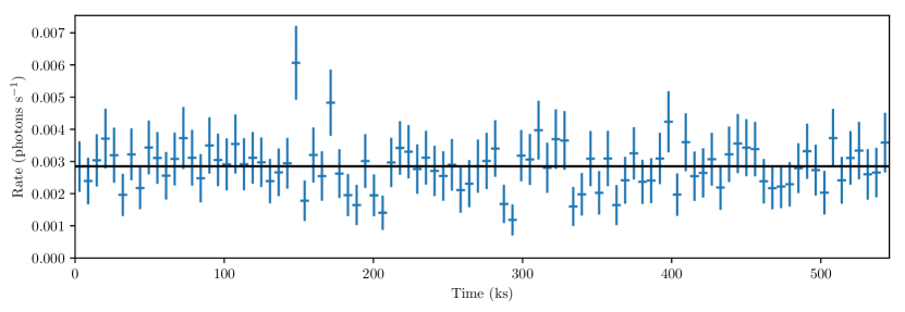
Figure A.1: Combined FPMA and FPMB 10–20 keV source light curve of the 2013 June 29 NuSTAR observation. The black line shows the average count rate, which has a total $\chi^{2}$ value of 88 for 93 DoF (the error bars are 1$\sigma$). The bin size is 5.8 ks (horizontal error bars), matching the orbital period of NuSTAR. The count rate has been corrected for Earth occultation periods and time filtering criteria (Section 2.1), which result in varying livetimes within each bin.

Before performing a detailed search for pulsed emission, we visually inspect the light curves. The light curve from the 2013 June 29 observation is shown in Figure A.1 as an example (the other light curves are similar). There are no indications of variability within individual observations. A priori, a detection is also unlikely given our favored model for SN 1987A and limited data quality. However, a rigorous search for pulsed emission is motivated by the importance of a potential detection and the fact that the expected spin period cannot be probed visually.

A.1 Data Reduction

The reduction of this data was performed separately and used the latest software at an earlier time of analysis, specifically NuSTARDAS 1.8.0 and CALDB version 20180126. We transform the timestamps of the events to Barycentric Dynamical Time (TDB) at the solar system barycenter using the task barycorr (for an overview of measures of time, see Eastman et al. 2010), with JPL Planetary Ephemeris DE-405.

We combine the data from the FPMA and FPMB modules, and restrict the energy range to 10–20 keV. Below 10 keV, Chandra images clearly show that the ER dominates. The optical depth through the ejecta is also very high below 10 keV (Section 5.5). The upper 20 keV limit is imposed to optimize the S/B.

We extract source photons from a circular region with a radius of 75″ pixels, which optimizes the signal-to-noise ratio. No background sample is necessary for the timing analysis. The source region contains a total of 22,381 events and the number of source events is estimated to be ${\sim}$10,000, assuming a spatially uniform background.

A.2 Timing Analysis

Overall, our timing method is similar to that of the Fermi pulsar search Einstein@Home (Clark et al., 2017). Here, we provide an overview of the method and motivate the choice of parameters.

The source extraction radius of 75″ is relatively large compared to the 18″ FWHM of the telescope, which implies that a large number of background events are included. This is not an issue because we assign a weight to each event based on the likelihood that it is produced by SN 1987A (Bickel et al., 2008; Kerr, 2011). The likelihood is computed by considering the position of the event, the background level, and the known point spread function of the telescope.

To test the significance of pulsed emission, we use the $H$-test introduced by de Jager et al. (1989). The test is named after Hart (1985) and belongs to the class of tests for uniformity on the circle (Rayleigh, 1919; Beran et al., 1969). The $H$-test is designed to be powerful for typical, general pulsar pulse profiles, which is useful when the pulse profile is unknown. The null cumulative distribution function for the $H$-statistic is accurately known from simulations (de Jager & Büsching, 2010). The $H$-statistic from different observations can be summed incoherently and its approximate null distribution is also known (de Jager & Büsching, 2010).

To reduce computational complexity, we divide the total exposure of 2.8 Ms into 32 time intervals with an average exposure of 90 ks. A search is performed on each interval separately and the test statistics are then combined incoherently. The incoherent summing over long timescales is possible because the timing accuracy of NuSTAR is stable to within ${\sim}2$ ms (Madsen et al. 2015; see Bachetti et al. 2021 for a recent significant improvement to $<100$ µs).

The neutron star spin is characterized by the period ($P$) and spin-down rate ($\dot{P}$). We search all periods from 30 ms to 1 ks. For reference, the temporal resolution of NuSTAR is 3 ms (Madsen et al., 2015) and the deadtime per event is 2.5 ms (Bachetti et al., 2015; Bachetti & Huppenkothen, 2018).

For each $P$, we search $\dot{P}$ from 0 to a maximum limit on $\dot{P}$. This limit is either set by the spin-down luminosity ($L$) or the spin-down age ($\tau_{\mathrm{sd}}$), depending on which is more constraining for a given $P$. The spin-down is related to the luminosity by

$$\dot{P}=\frac{5LP^{3}}{8\pi{}^{2}MR^{2}},$$ (A1)

where $M$ is neutron star mass and $R$ the neutron star radius. We adopt parameter values of $L=$10,000 L_☉, $M=1.4$ M_☉, and $R=12$ km (Özel & Freire, 2016). This spin-down luminosity is much higher than the bolometric limit on the order of 100 L_☉ (Alp et al., 2018b), but the spin-down luminosity could potentially be much higher than the bolometric luminosity (Abdo et al., 2013; Caraveo, 2014).

The spin-down age is given by

$$\tau_{\mathrm{sd}}=\frac{P}{2\dot{P}}$$ (A2)

and we choose the limit $\tau_{\mathrm{sd}}>10^{8}$ s (${\sim}3$ years). With the aforementioned values, the limit on $\dot{P}$ from Eq. (A1) is $<6\times 10^{-10}P^{3}$ s^-3 and the limit from Eq. (A2) is $<5\times{}10^{-9}P$ s^-1. The spin-down must fulfill both criteria, implying a sufficiently low $L$ to be consistent with multi-wavelength observations and high enough $\tau_{\mathrm{sd}}$ to be reasonably consistent with the age of SN 1987A. For completeness, we also search $-\dot{P}$ for each $\dot{P}$ to allow for potential spin-up.

A.3 Results

We detect no pulsed emission from SN 1987A and verify that the observed $H_{T}$ distribution is consistent with the null distribution. Instead, we put a constraint on the pulsed fraction of the emission in the 10–20 keV range. We compute the limit by simulating a pulsed signal. The signal is modeled by a single Gaussian with a duty cycle of 20 % (FWHM).

Assuming the 10–20 keV emission to be from a PWN, the 3$\sigma{}$ upper limit on the source pulsed fraction is 15 % (background subtracted). Importantly, however, the 10–20 keV range certainly includes photons from ER interactions. This implies that the upper limit on the pulsed fraction of the compact object emission is less constraining than 15 %. For example, if the thermal-to-PWN flux ratio is $>7$, the pulsed fraction is completely unconstrained since a 100 % pulsed fraction would go undetected.

Appendix B Radioactive K$\alpha$ Lines

Table 7: XMM-Newton Observations Used for Limits on Radioactive K$\alpha$ Lines

Obs. ID	Start Date	Epoch	pn Exp.	MOS1 Exp.	MOS2 Exp.
	(YYYY-mm-dd)	(d)	(ks)	(ks)	(ks)
0115690201	2000-01-19	4713	22	$\cdots$	$\cdots$
0115740201	2000-01-21	4715	33	43	32
0104660101	2000-09-17	4955	04	$\cdots$	$\cdots$
0104660301	2000-11-25	5024	$\cdots$	21	21
0083250101	2001-04-08	5158	14	13	13
0144530101	2003-05-10	5920	57	58	54

Note. — All cameras were not operating simultaneously in science mode during some observations in the early XMM-Newton cycles.

We search early XMM-Newton pn and MOS data for the ⁵⁵Mn 5.9 and ⁴⁴Sc 4.1 keV lines. Only observations from 2000 to 2003 (Table 7) are used because the thermal emission from the ER becomes overwhelming at later times. The data reduction is similar to the reduction for the primary analysis (Section 2.2). The differences are that we use both pn and MOS data, perform no pile-up correction due to the lower fluxes, and choose smaller source radii of 10–25″ to improve S/B. Furthermore, we bin to a minimum of 1 count per bin and use the $C$ statistic (Cash, 1979) because of the lower number of photons. A background subtraction is not performed for these fits. Technically, XSPEC employs the $W$ statistic for these fits, but it is activated using the statistic cstat command.

B.1 The 5.9 keV ${}^{55}Mn$ Line

Our methods follow Leising (2006), who perform an analogous analysis using Chandra data. Focusing first on the ⁵⁵Fe chain, we limit the energy range to 4–8 keV and fit a model consisting of a PL and a Gaussian line. The power-law normalization, power-law photon index, and line flux are left free. The line energy is frozen to 5.9 keV and line width (represented by $\sigma$) is frozen to 0.06 keV (3000 km s^-1 Doppler width). We find a 3$\sigma$ upper limit on the line flux of $4.2\times{}10^{-7}$ photons s^-1 cm^-2. This is similar to the approximate limit of $<3\times{}10^{-7}$ photons s^-1 cm^-2 found by Leising (2006).

The ⁵⁵Mn line is absorbed by the ejecta to a varying degree sensitively depending on the spatial ⁵⁵Mn distribution. The amount of absorption is modeled by an average “effective” optical depth. At the relevant epochs, only the outermost ⁵⁵Mn on the near side is observable (Alp et al., 2018a, 2019). Therefore, dedicated detailed computations are necessary to estimate the amount of absorption. Leising (2006) estimated the amount of absorption of the 5.9 keV line by the ejecta using the 10HMM SN model (Pinto & Woosley, 1988). This model is one-dimensional and has additional mixing introduced by hand. It was designed to successfully match many observables (McCray, 1993), in particular the X-ray and gamma-ray properties during the first few years (Alp et al., 2019). At the relevant epochs, the effective optical depth is ${\sim}1.2$ at 5.9 keV for the modeled ⁵⁵Fe distribution. Combining this with the flux limit results in a $3\sigma$ upper limit on the initial ⁵⁵Fe mass of $4.2\times{}10^{-4}$ M_☉.

However, we note that there is a hint of a line at 5.9 keV in the data. Quantitatively, the estimated flux is $1.2_{-0.9}^{+1.0}\times{}10^{-7}$ photons s^-1 cm^-2 with a 1$\sigma$ confidence level. This indicates that there might be a weak detection of the line, or possibly slight contamination from the ⁵⁵Mn pn energy calibration source (Strüder et al., 2001). We inspect the residuals but are unable to draw a firm conclusion. If astrophysical, the flux would point toward an initial ⁵⁵Fe mass of $1.2_{-0.9}^{+1.0}\times{}10^{-4}$ M_☉. We stress that the interval is a purely statistical 1$\sigma$ interval. Systematic uncertainties are certainly also significant, particularly due to uncertainties in the amount of absorption. For reference, nucleosynthesis simulations predict ⁵⁵Fe masses in the range 1–20$\times{}10^{4}$ M_☉ (Leising, 2006; Popov et al., 2014; Sieverding et al., 2020).

B.2 The 4.1 keV ${}^{44}Sc$ Line

The analysis of the ⁴⁴Sc 4.1 keV line is analogous to that of the ⁵⁵Mn 5.9 keV line. For ⁴⁴Sc, we use the 3–5.5 keV range, shift the line to 4.1 keV, and repeat the same procedure. The 3$\sigma$ upper limit on the line flux is $3.0\times 10^{-7}$ photons s^-1 cm^-2. We note that He-like Ca could produce K-shell lines near 4.1 keV, but we see no signs of any line around 4.1 keV in the residuals. The thermal X-ray emission rapidly rises toward lower energies, which reduces the sensitivity. Since the initial ⁴⁴Ti mass is known to be ${\sim}1.7\times{}10^{-4}$ M_☉ (Section 4.7), we compute the unattenuated flux to be $7.9\times 10^{-7}$ photons s^-1 cm^-2. Thus, the 4.1 keV flux limit does not constrain any parameters since it implies an effective optical depth of $>1$, which clearly is consistent with the value of ${\sim}3$ obtained from the 10HMM model.

Appendix C Systematic Uncertainties

The calibration of X-ray instruments is known to be slightly inaccurate with errors of approximately 5–10 % (Plucinsky et al., 2008, 2017; Ishida et al., 2011; Madsen et al., 2017). In general, the calibration errors are energy-dependent, implying that spectral shapes are affected in addition to the overall normalization. We introduce free constants between different instruments when fitting simultaneously, which capture overall normalization errors. This approach does not address the energy dependence, but is still conventionally used in X-ray analyses.

The calibrations are known to be variable and depend on epoch, observing conditions, and underlying spectrum. Therefore, we investigate the spectral difference between NuSTAR and XMM-Newton/pn using our data. We do this by fitting a simplified version of the thermal shock model. This model is the same as the standard model but with only one shock component. This is sufficient because we only perform the comparison in a reduced energy range from 3–8 keV. To quantify the calibration differences, the temperature of this single component is untied between NuSTAR and pn (with $\tau$ and the EM remaining tied).

We fit this model to all epochs and provide the resulting temperatures and fit statistics in Table 8. The average NuSTAR temperature ($k_{\mathrm{B}}T_{\mathrm{AB}}$) is 2.79 keV compared with the average pn temperature ($k_{\mathrm{B}}T_{\mathrm{pn}}$) of 2.39 keV. This difference is clearly systematic as all $T_{\mathrm{AB}}$ are significantly higher than $T_{\mathrm{pn}}$.

When the temperatures are tied, the average cross-normalization between NuSTAR ($C_{\mathrm{AB}}$) and pn ($C_{\mathrm{pn}}$) is $0.88C_{\mathrm{pn}}=C_{\mathrm{AB}}$. The corresponding factor is 0.71 when the temperatures are untied. Consequently, the absolute magnitude difference between NuSTAR and pn is approximately 0.88. The remaining difference when the temperatures are untied is primarily due to the connection between the temperature and the EM. This shows that both the normalization and spectral shapes are different between NuSTAR and pn.

Table 8 also shows the improvement in fit statistics obtained by untying the NuSTAR and pn temperatures compared with tying the temperatures. The average difference at each epoch of $\Delta\chi^{2}\approx{}-16$ shows that the calibration differences are significant. This value is only computed from the goodness within the fitted 3–8 keV energy range and would be higher if a broader energy range was used.

We note that the third NuSTAR and pn epochs are separated by only one day. Any temporal evolution within this time interval is certainly negligible. The fits from this epoch show similar results to other epochs, which implies that the differences introduced by assuming simultaneity within the epochs likely are small compared to the systematic calibration differences.

Due to the calibration uncertainties, we omit the pn data from the detailed spectral analysis to avoid biases. We motivate this further, and explore the effects of including pn data and a number of other choices for managing the calibration uncertainties in detail in Appendix D below. Finally, we also note that the pn data is corrected for modest levels of pile-up (Section 2.2), which could affect the accuracy.

In addition to the systematic differences between NuSTAR and pn, the analysis is also affected by calibration uncertainties between pn and RGS at low energies. The differences between these instruments have previously been studied by dedicated calibration programs (Plucinsky et al., 2008, 2017). Small differences are clearly visible in the observations of SN 1987A (see Figures in Appendix D), but these cannot be easily modeled due to the more complex spectrum at low energies. A simplified method of avoiding part of the problem is to raise the lower limit of the pn energy range slightly. We choose 0.8 keV as a trade-off between using as much data as possible and introducing calibration tensions into the fits.

Table 8: Comparison of Fitted Temperatures Between NuSTAR and XMM-Newton/pn

Epoch	$\Delta{}t$	$k_{\mathrm{B}}T_{\mathrm{AB}}$	$k_{\mathrm{B}}T_{\mathrm{pn}}$	$T_{\mathrm{pn}}/T_{\mathrm{AB}}$	$\chi^{2}_{\mathrm{AB}}/\mathrm{DoF}$	$\chi^{2}_{\mathrm{pn}}/\mathrm{DoF}$	$\Delta\chi^{2}$
(d)	(d)	(keV)	(keV)
01,93320	00 $-92$00	0$2.78_{-0.15}^{+0.12}$0	0$2.33_{-0.10}^{+0.11}$0	0.840	297/294=1.01	98/66=1.49	$-21.40$
01,93720	00 $-52$00	0$2.79_{-0.16}^{+0.15}$0	0$2.33_{-0.10}^{+0.11}$0	0.840	183/199=0.92	98/66=1.49	$-19.25$
01,94240	0000 $1$00	0$2.65_{-0.15}^{+0.18}$0	0$2.32_{-0.10}^{+0.11}$0	0.88	163/165=0.99	98/66=1.49	$-10.09$
01,96230	00 $199$00	0$2.64_{-0.11}^{+0.12}$0	0$2.35_{-0.10}^{+0.11}$0	0.890	221/241=0.92	98/66=1.49	$-10.79$
01,99200	0 $-221$00	0$2.77_{-0.12}^{+0.10}$0	0$2.40_{-0.10}^{+0.11}$0	0.870	316/309=1.02	64/67=0.96	$-16.46$
01,99780	0 $-163$00	0$2.83_{-0.10}^{+0.11}$0	0$2.38_{-0.10}^{+0.11}$0	0.840	331/338=0.98	64/67=0.96	$-23.71$
0 10,0210	0 $-120$00	0$2.78_{-0.12}^{+0.10}$0	0$2.44_{-0.10}^{+0.12}$0	0.880	264/263=1.00	65/67=0.97	$-13.02$
0 12,1470	00 $182$00	0$3.10_{-0.13}^{+0.15}$	0$2.56_{-0.18}^{+0.22}$	0.830	379/353=1.17	70/54=1.30	$-13.06$

Note. — Fitting a single shock component to the 3–8 keV range. The temperature $T_{\mathrm{AB}}$ is inferred from the NuSTAR data whereas $T_{\mathrm{pn}}$ is from pn data. The fits to the XMM-Newton data show a rather variable goodness of fit at different epochs, likely primarily driven by random fluctuations and to a lesser extent by the spectral evolution. The data quality and reduction process are very similar for the different XMM-Newton epochs.

In addition to the instrumental calibration errors, there are systematics introduced by the data reduction and methods. For example, Frank et al. (2016) also analyzed the XMM-Newton observations up to 10,141 d. We find better agreement within a few percent at 0.5–2 keV and at earlier epochs (around 8000 d), but up to 10 % higher 3–8 keV fluxes at later times. There is a large number of factors that could contribute to these differences: source and background regions; data calibration version; choice of underlying model; free parameters; ISM and model abundances; amount of absorption; cross sections; and pile-up corrections.

For these reasons, we add a systematic uncertainty to our X-ray fluxes. This is added in quadrature to the systematic error in Figure 4, but we report both separately in tables. We adopt a fiducial systematic uncertainty of 8 % (of the total flux), which we believe is a reasonable estimate. This particular value is the typical difference we find in our comparisons between independent analyses. It also agrees with cross-calibration programs between different instruments (e.g. Plucinsky et al. 2017; Madsen et al. 2017). We do not rely on this value for any quantitative analysis. The purpose is solely to serve as a reminder of the systematics, which are often left implicit.

Finally, we note that these systematics only apply to comparisons between parameters from different instruments, data reductions, or methods. The systematic errors are likely significantly lower for analyses of homogeneously estimated parameter values. Importantly, this implies that the fluxes derived from the same instrument (and analysis) are comparable.

Appendix D Alternative Set-ups for the Spectral Analysis

Table 9: Fit Results for Different Data Sets and Models

Model	RGS	pn	NuS.	$\chi^{2}_{3}/\mathrm{DoF}_{3}$	$\chi^{2}_{\Sigma}{}/\mathrm{DoF}_{\Sigma}{}$	$k_{\mathrm{B}}T_{1}$	$k_{\mathrm{B}}T_{2}$	$k_{\mathrm{B}}T_{3}$
						(keV)	(keV)	(keV)
2 shocks${}^{\text{I}}$	✓	✓	✓	$2559/1749=1.46$	$20741/14520=1.43$	$0.71$	$\cdots$	$3.06$
2 shocks	✓	✗	✓	$2093/1623=1.29$	$17223/13515=1.27$	$0.66$	$\cdots$	$3.25$
2 shocks	✗	✓	✓	$573/328=1.75$	$5815/3776=1.54$	$0.76$	$\cdots$	$3.14$
2 shocks	✓	✓	✗	$\cdots$	$17126/11709=1.46$	$0.70$	$\cdots$	$2.66$
3 shocks${}^{\text{II}}$	✓	✓	✓	$2059/1746=1.18$	$17111/14496=1.18$	$0.54$	$0.96$	$3.39$
3 shocks${}^{\text{III}}$	✓	✗	✓	$1771/1620=1.09$	$14810/13491=1.10$	$0.53$	$0.97$	$3.84$
3 shocks	✗	✓	✓	$451/325=1.39$	$4676/3752=1.25$	$0.63$	$0.98$	$3.58$
3 shocks	✓	✓	✗	$\cdots$	$13694/11685=1.17$	$0.52$	$0.93$	$2.82$
$T_{\mathrm{X}}=0.88T_{3}$${}^{\text{IV}}$	✓	✓	✓	$2019/1746=1.16$	$16756/14496=1.16$	$0.52$	$0.94$	$3.43$

Note. — The data sets used are indicated by the checkmarks and crosses. The fit statistics for the third epoch when the NuSTAR and XMM-Newton observations are separated by one day are given by $\chi^{2}_{3}/\mathrm{DoF}_{3}$. The summed fit statistics across all epochs are given by $\chi^{2}_{\Sigma}{}/\mathrm{DoF}_{\Sigma}{}$. The temperatures are the averages across epochs for the different shock components in order of increasing temperature, identified by the subscripts. The last model has different NuSTAR and XMM-Newton temperatures for the hottest component. The NuSTAR temperature is $T_{\mathrm{3}}$, whereas the XMM-Newton temperature is $T_{\mathrm{X}}$. The statistical errors (not shown) for the temperatures vary by approximately a factor of 2 for the different set-ups. More data generally reduce the uncertainties and the different data sets naturally primarily affect the components within the energy ranges of the instruments.

In this section, we explore different possibilities for handling the cross-calibration uncertainties in the spectral analysis. We try different spectral models, treatments of instrument differences, and data sets. A summary is provided in Table 9 and the fits are described below. Importantly, even though the best-fit values are slightly different, our main conclusions remain unchanged regardless of how the data are analyzed.

D.1 Models Used for Comparisons

The models we present here are the standard model with three shocks and a simplified version with only two shock components. We fit this model to RGS, pn, and NuSTAR data simultaneously, as well as separately to data from only two of the instruments. This leads to four possible set-ups for each of the models. All parameters apart from constant cross-normalization factors are tied between the instruments in these fits. The fitted energy ranges are the same as presented in Section 3.

In addition to the fits with two and three shock components, we investigate a variation of the three-shock model. For this model, the temperatures of the hottest component are coupled as $T_{\mathrm{X}}=0.88T_{3}$, where $T_{3}$ is the NuSTAR temperature and $T_{\mathrm{X}}$ is the XMM-Newton temperature. The factor 0.88 is obtained from the fit to the overlapping 3–8 keV region of the third epoch at 9424 d (Table 8). This version of the model with different temperatures for the hottest components is only fitted to RGS, pn, and NuSTAR data simultaneously.

There are a number of other possible variations for connecting the NuSTAR and pn data. In addition to the fits presented below, we have explored constraining the cross-normalizations, completely decoupling the temperatures, and additionally untying the EMs of the hottest components. The trend is naturally that gradually increasing the amount of freedom improves the fit quality, but the results are similar for all set-ups.

D.2 Results

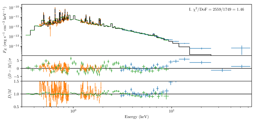
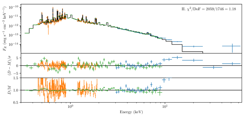
Figure D.1: NuSTAR (blue), RGS (orange), and pn (green) spectra together with the best-fit model (black) from the third epoch at 9424 d. The four subfigures (continues on the next page) show different set-ups (Table 9): Two-shock model fitted to all data (I). Three-shock model fitted to all data (II). Three-shock model fitted to NuSTAR and RGS with pn overplotted (III). This is the standard model used throughout the main text. Three-shock model fitted to all data with the temperatures of the hottest component rescaled as $T_{\mathrm{X}}=0.88T_{3}$ between XMM-Newton and NuSTAR (IV; Appendix C). The top panels in the individual subfigures show the spectra, the middle panels show the normalized residuals, and the bottom panels show the data-to-model ratio. The two upper panels of each figure are analogous to Figure 6. The pn data are shown from 0.3 keV, but only 0.8–10 keV data are used for the analysis throughout the paper.

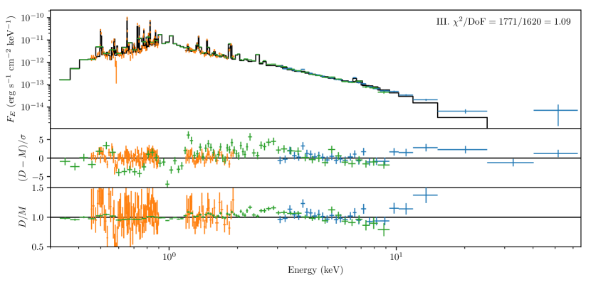
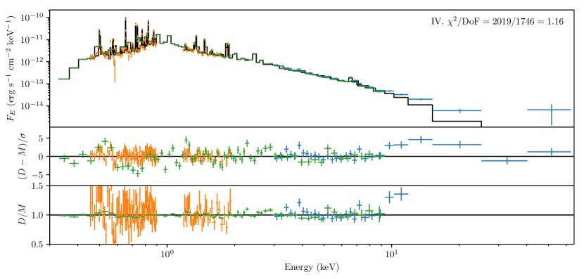
Figure D.1: (Continued.)

The fit statistics and temperatures of the above set-ups are provided in Table 9. We present the fit statistics to all data combined, the average temperatures, and the goodness of fits to the third epoch (9424 d; NuSTAR and XMM-Newton are separated by one day). We also show fits of four of the models in Figure D.1 where the models are identified by Roman numerals (see Table 9).

First, we compare Models I and II. These are the models with two and three shock components, respectively, that are fitted to data from NuSTAR, RGS, and pn. It is clear that two components (Model I) are insufficient to model the combined spectrum and that including a third component (Model II) results in a substantial improvement in the goodness of fit. Specifically, the improvement for the third epoch alone is $\Delta\chi^{2}=-500$ for an additional 3 DoF, and $\Delta\chi^{2}=3630$ for an additional 24 DoF across all epochs combined. The reason for the inferior fit using two components is primarily driven by the $<2$ keV range, as can be seen in Figure D.1. This is also clear from the temperatures of the two cooler components of the three-shock model. Both cool components have temperatures below ${\sim}$1 keV and primarily influence the RGS energy range. The first two subfigures of Figure D.1 also show that the addition of a third component does not significantly change the broadband model continuum shape. This implies that conclusions regarding the continuum are relatively independent of the third shock component. However, a third component is clearly motivated by the statistical improvement. We note that improved fits can be achieved by allowing for more freedom by freeing the constant parameters (Section 3.2) or more conservative data filtering criteria (which reduces the number of photons; e.g. Sun et al. 2021), but exploring all these possibilities are not within the current scope.

Figure D.1 subfigure II can also be compared with subfigure III. Both use the same standard three-shock model. The difference between these models is that Model II is fitted to all data, whereas Model III is fitted to NuSTAR and RGS data. We note that Model III is the primary standard model used for the main analysis. The pn data in subfigure III have been overplotted and only rescaled by a factor of 0.95 to minimize the residuals. It is clear from the residuals that there are systematic offsets between the NuSTAR and pn data (as quantified in Appendix C above). This is especially clear in the overlapping region. Furthermore, the pn data are in excess of the model in the 3 keV region, which is a consequence of the differences in spectral slope. The consequences of these difference can be seen in the residuals of subfigure II and the worse fit statistic.

Given the known differences between NuSTAR and pn, we also show the model variant with the NuSTAR and XMM-Newton temperatures rescaled as $T_{\mathrm{X}}=0.88T_{3}$ (Model IV). Model IV can be compared to Models II and III in Figure D.1. The rescaling of temperatures alleviates a significant part of the tension but still drastically reduces the overall quality of the fit when compared to fits without pn data. Comparing Models III and IV, introducing the pn data to the fits introduces 1005 DoF in total across all epochs (Table 9). The change in total $\chi^{2}$ is 1946, implying that the fit is significantly worse despite the $T_{\mathrm{X}}=0.88T_{3}$ scaling. This is not surprising since the calibration errors between all three instruments are more complicated than what can be captured by our simplified treatment.

In addition to the decrease in overall fit quality for Model IV, the average cross-normalization constant between the NuSTAR and XMM-Newton data is 0.82. These fits use the three-shock model, but NuSTAR is quite insensitive to the two cooler components. This means that the EM of the hottest component is degenerate with the cross-normalization constant, which implies that the connection between the NuSTAR and pn data is relatively weak. Consequently, the hottest shock components are largely decoupled between NuSTAR and pn, which partly defeats the purpose of including the pn data. In light of this, we conclude that adding the pn data worsens the fit quality, introduces biases, and adds little information since the components are required to be relatively uncoupled.

Despite the above arguments, including pn data remains a possible alternative. I principle, it is possible that the pn data are more accurate than NuSTAR data. However, the inconsistencies in the overlapping region between NuSTAR and pn show that there must be significant calibration errors. The excess above 10 keV in NuSTAR, which is more pronounced when pn data are included, cannot be a result of instrumental calibration since the ratio between the data and model is much higher than $10$ %. It is possible that the fit attempts to capture calibration inconsistencies at the expense of producing an artificial excess above 10 keV. This could happen if both the instrumental inconsistencies and artificial excess are of comparable statistical significance.

Importantly, including pn data do not affect the scientific conclusions qualitatively. The pn data lowers the temperature of the hottest component from ${\sim}$4 to ${\sim}$3–3.4 keV. Naturally, this leads to an increased excess in the NuSTAR data above 10 keV. This does not imply that the origin of such an excess is physically different. Even in this case, we argue that it most likely is the hottest part of the thermal emission. Simply adding a fourth thermal component to the model does not provide stable fits as the temperatures vary irregularly across epochs. We note that the continuous temperature model has sufficient freedom to allow for a broader temperature distribution. This model fits the data well and is discussed in Section D.3 below.

Instead, to characterize the shapes of the NuSTAR spectra, we fit a two-shock model to all NuSTAR epochs with no other data sets. The fitted temperatures are $1.8\pm 0.3$ and $5.9\pm 0.7$ keV (these intervals are standard deviations among the eight epochs) with a total fit statistic of $\chi^{2}=2599$ for 2771 DoF. We also inspect the residuals and find that the fits are very good. This shows that the NuSTAR spectra can be well-fitted with a thermal model with temperatures up to ${\sim}$6 keV. Temperatures around 6 keV are not unreasonably high since a faint, hot component with temperatures of up to 20–49 keV is expected from the reverse shock (Section 5.1.3).

Moreover, in Section 4.5, we show that the NuSTAR data alone do not favor the inclusion of an additional PL component, implying that thermal models are fully sufficient to model the NuSTAR data. This mean that there is no support for two physically distinct components based on the NuSTAR data alone. Therefore, it seems more likely that an excess, which is more significant when pn data are included, is a result of calibration uncertainties or a high-energy tail of the thermal distribution. Based on the above discussion, we favor excluding the pn data from the spectral analysis, while noting that including the pn data would not affect the conclusions qualitatively.

D.3 Implication of Adding pn Data for the Continuous Model

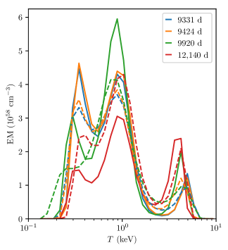
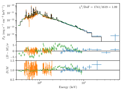
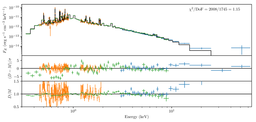
Figure D.2: Upper left panel: Fitted EM distributions (Eq. 1) for the continuous shock temperature model. Solid lines are for the fits to only RGS and NuSTAR data (same as in Figure 9). Dashed lines are the corresponding fits to all data, including pn. Only a cross-normalization is allowed to vary between the instruments. Only four epochs are shown for visual clarity but the remaining epochs show similar behaviors. Upper right panel: NuSTAR (blue), RGS (orange), pn (green) and the model (black) spectra from the third epoch at 9424 d. The fit is only performed to NuSTAR and RGS data. The pn data are only overplotted and rescaled by 1.06 to minimize the residuals. Lower panel: Same as upper right but also fitted to the pn data. The upper-right fit corresponds to the solid orange line in the upper left plot, whereas the lower-panel fit corresponds to the dashed orange line. As in Figure D.1, the pn data are shown from 0.3 keV, but only 0.8–10 keV data are used for the analysis throughout the paper.

It is also illuminating to explore fits of the continuous temperature model in addition to the discrete temperature models above. We show the results of fits of the continuous temperature model to RGS, pn, and NuSTAR data in Figure D.2. Only a cross-normalization constant is allowed to vary between the instruments (standard set-up). The results are qualitatively similar to fits without the pn data, and primarily show a well-separated high-temperature peak and a broader, possibly bimodal, peak below 2 keV. The differences are expected due to the large amount of freedom in the fits and the amount of data added by pn. This further strengthens the argument that the pn data do not qualitatively affect the conclusions.

Figure D.2 also shows spectra and residuals of the continuous model for the third epoch at 9424 d. We show fits both with and without the pn data. The temperature distributions for these models both show contributions up to approximately 5 keV, above which the distributions quickly decline. It is clear that an excellent fit can be achieved using the continuous model when pn data are not included. In particular, we note that the slight excess visible above 10 keV is well-captured when the model includes a faint temperature tail to ${\sim}$6 keV.

The fit including the pn data is also relatively good. It is evident that the main issues for this fit are the tensions between the instruments, as can be seen in the overlapping regions. This can also be seen in the fit statistics. When pn data are included, the fit statistic for the third epoch increases by 267 for 126 DoF, for a total increase of 1954 for 1005 DoF across all epochs. Despite the tensions, the fit is reasonable and the resulting temperature distribution is very similar to when pn data are excluded.

This further corroborates the conclusion that a purely thermal model is sufficient. Of course, the investigations above do not prove that other components are excluded. They only show that additional components are not necessary.

Appendix E XMM-Newton Fluxes

Table 10: XMM-Newton Fluxes

Obs. ID	Epoch	$F_{\text{0.45--0.7}}$	$F_{\text{0.5--2}}$	$F_{\text{3--8}}$	$F_{\text{0.5--8}}$
	(d)	($10^{-13}$ erg s-1 cm-2)	($10^{-13}$ erg s-1 cm-2)	($10^{-13}$ erg s-1 cm-2)	($10^{-13}$ erg s-1 cm-2)
0144530101	5920	$1.78_{-0.09}^{+0.07}\pm 0.14$	$8.0_{-0.1}^{+0.1}\pm 0.6$	$1.66_{-0.02}^{+0.02}\pm 0.13$	$10.5_{-0.2}^{+0.2}\pm 0.8$
0406840301	7268	$5.75_{-0.12}^{+0.10}\pm 0.46$	$34.1_{-0.2}^{+0.2}\pm 2.7$	$3.93_{-0.02}^{+0.02}\pm 0.31$	$40.7_{-0.3}^{+0.3}\pm 3.3$
0506220101	7627	$7.01_{-0.09}^{+0.10}\pm 0.56$	$44.4_{-0.2}^{+0.2}\pm 3.6$	$5.32_{-0.02}^{+0.02}\pm 0.43$	$52.9_{-0.3}^{+0.3}\pm 4.2$
0556350101	8012	$8.39_{-0.14}^{+0.09}\pm 0.67$	$54.9_{-0.2}^{+0.2}\pm 4.4$	$6.35_{-0.03}^{+0.03}\pm 0.51$	$66.2_{-0.3}^{+0.3}\pm 5.3$
0601200101	8327	$8.71_{-0.10}^{+0.09}\pm 0.70$	$62.6_{-0.2}^{+0.2}\pm 5.0$	$7.73_{-0.03}^{+0.03}\pm 0.62$	$77.6_{-0.2}^{+0.3}\pm 6.2$
0650420101	8693	$9.44_{-0.13}^{+0.12}\pm 0.76$	$70.7_{-0.3}^{+0.3}\pm 5.7$	$9.45_{-0.04}^{+0.04}\pm 0.76$	$86.9_{-0.4}^{+0.4}\pm 7.0$
0671080101	9048	$9.78_{-0.13}^{+0.11}\pm 0.78$	$76.4_{-0.2}^{+0.3}\pm 6.1$	$10.91_{-0.04}^{+0.04}\pm 0.87$	$95.0_{-0.3}^{+0.4}\pm 7.6$
0690510101	9423	$9.87_{-0.10}^{+0.10}\pm 0.79$	$80.1_{-0.3}^{+0.2}\pm 6.4$	$12.34_{-0.04}^{+0.05}\pm 0.99$	$103.2_{-0.3}^{+0.2}\pm 8.3$
0743790101	10,141	$9.13_{-0.09}^{+0.09}\pm 0.73$	$79.9_{-0.2}^{+0.3}\pm 6.4$	$14.29_{-0.05}^{+0.05}\pm 1.14$	$103.5_{-0.4}^{+0.4}\pm 8.3$
0763620101	10,492	$8.59_{-0.08}^{+0.09}\pm 0.69$	$78.9_{-0.3}^{+0.2}\pm 6.3$	$15.36_{-0.06}^{+0.06}\pm 1.23$	$104.7_{-0.4}^{+0.4}\pm 8.4$
0783250201	10,845	$8.56_{-0.12}^{+0.08}\pm 0.68$	$76.3_{-0.3}^{+0.3}\pm 6.1$	$16.12_{-0.06}^{+0.06}\pm 1.29$	$102.1_{-0.4}^{+0.4}\pm 8.2$
0804980201	11,192	$7.67_{-0.08}^{+0.07}\pm 0.61$	$73.6_{-0.3}^{+0.4}\pm 5.9$	$16.66_{-0.08}^{+0.08}\pm 1.33$	$98.5_{-0.5}^{+0.5}\pm 7.9$
0831810101	11,965	$6.64_{-0.13}^{+0.13}\pm 0.53$	$65.2_{-0.4}^{+0.4}\pm 5.2$	$17.27_{-0.11}^{+0.11}\pm 1.38$	$90.7_{-0.6}^{+0.6}\pm 7.3$

Note. — The flux $F_{a\text{--}b}$ denotes the flux from $a$ to $b$ keV. Asymmetric error bars are statistical and the symmetric uncertainties are systematic (Appendix C).

We provide fluxes in four energy bands for all XMM-Newton observations in Table 10. These fluxes, except for the full 0.5-8 keV flux, are plotted in Figure 4. The 0.45–0.7 keV range is dominated by the strong N vii Ly$\alpha$ (0.5003 keV) and O viii Ly$\alpha$ (0.6537 keV) lines. In the literature, 0.5–2 keV is commonly referred to as the “soft” band, while 3–8 keV is the “hard” band.

Appendix F Best-Fit Parameters

Table 11 provides all best-fit parameters for fits using the standard three-shock model (Sections 3.1 and 4.2). The temperatures are shown in Figure 7. We note that all $\tau_{2}$ and the last epoch $\tau_{1}$ only have lower limits. There also appears to be slight degeneracies between $\tau$ and EM between different shock components, which can be seen by the difference at 12,140 d relative to the other epochs. However, the decrease in $T_{3}$ in the last epoch appears robust. This is supported by the light curves, hardness ratios, and continuous model fits.

In Table 12, we provide the observed (absorbed) fluxes of the individual components and goodness-of-fit measures. These fluxes are the bolometric fluxes of the components. Consequently, they are much more uncertain than the fluxes in energy bands (Table 5) because the component fluxes are more sensitive to the underlying model.

Table 11: Best-Fit Parameters of the Three-Shock Model to NuSTAR and RGS Data

Group	Epoch	$k_{\mathrm{B}}T_{1}$	$k_{\mathrm{B}}T_{2}$	$k_{\mathrm{B}}T_{3}$	$\tau_{1}$	$\tau_{2}$	$\tau_{3}$	EM1	EM2	EM3
	(d)		(keV)			($10^{12}$ s cm-3)			($10^{58}$ cm-3)
1	9331	$0.52_{-0.03}^{+0.02}$	$0.98_{-0.05}^{+0.05}$	$4.1_{-0.2}^{+0.4}$	$0.92_{-0.11}^{+0.17}$	$>2$	$0.33_{-0.08}^{+0.29}$	$14.9_{-0.5}^{+0.8}$	$11.8_{-0.9}^{+1.1}$	$3.5_{-0.8}^{+0.6}$
2	9372	$0.50_{-0.02}^{+0.02}$	$0.96_{-0.06}^{+0.02}$	$3.7_{-0.2}^{+0.2}$	$0.97_{-0.13}^{+0.58}$	$>2$	$0.36_{-0.08}^{+0.21}$	$14.5_{-1.0}^{+0.7}$	$11.4_{-0.8}^{+1.1}$	$4.3_{-0.7}^{+0.7}$
3	9424	$0.51_{-0.04}^{+0.03}$	$0.97_{-0.05}^{+0.06}$	$3.8_{-0.2}^{+0.4}$	$0.93_{-0.13}^{+0.33}$	$>9$	$0.34_{-0.08}^{+0.39}$	$14.7_{-1.0}^{+0.8}$	$11.7_{-0.9}^{+1.0}$	$3.8_{-1.0}^{+0.6}$
4	9623	$0.52_{-0.02}^{+0.02}$	$0.99_{-0.02}^{+0.03}$	$4.0_{-0.2}^{+0.4}$	$0.95_{-0.05}^{+0.20}$	$>2$	$0.27_{-0.06}^{+0.10}$	$15.0_{-0.8}^{+0.5}$	$11.9_{-0.8}^{+1.0}$	$3.2_{-0.5}^{+0.3}$
5	9920	$0.55_{-0.01}^{+0.02}$	$0.98_{-0.01}^{+0.04}$	$3.9_{-0.1}^{+0.1}$	$0.86_{-0.09}^{+0.13}$	$>4$	$0.36_{-0.09}^{+0.20}$	$12.4_{-0.9}^{+0.7}$	$12.9_{-1.0}^{+0.9}$	$3.8_{-0.3}^{+0.5}$
6	9976	$0.55_{-0.03}^{+0.03}$	$0.98_{-0.02}^{+0.04}$	$4.1_{-0.2}^{+0.3}$	$0.85_{-0.12}^{+0.11}$	$>4$	$0.36_{-0.10}^{+0.32}$	$12.4_{-0.9}^{+1.4}$	$12.9_{-1.1}^{+1.0}$	$3.8_{-0.7}^{+0.5}$
7	10,021	$0.55_{-0.02}^{+0.02}$	$0.98_{-0.05}^{+0.02}$	$4.0_{-0.2}^{+0.2}$	$0.93_{-0.12}^{+0.22}$	$>5$	$0.26_{-0.06}^{+0.08}$	$12.4_{-1.2}^{+0.8}$	$12.8_{-1.0}^{+1.1}$	$3.5_{-0.4}^{+0.7}$
8	12,140	$0.49_{-0.09}^{+0.06}$	$0.98_{-0.07}^{+0.05}$	$3.5_{-0.1}^{+0.1}$	$>0.8$	$>2$	$0.51_{-0.14}^{+0.23}$	$6.9_{-0.8}^{+0.8}$	$10.2_{-1.1}^{+1.2}$	$7.6_{-1.0}^{+0.9}$

Note. — The subscripts on the parameters in the header refer to the three individual shock components in terms of increasing temperature. The goodness-of-fit measures of these fits are provided in Table 12.

Table 12: Observed Bolometric Fluxes of the Shock Components in Table 11

Group	Epoch	$F_{1}$	$F_{2}$	$F_{\text{3}}$	$\chi^{2}/\mathrm{DoF}$
	(d)	($10^{-13}$ erg s-1 cm-2)	($10^{-13}$ erg s-1 cm-2)	($10^{-13}$ erg s-1 cm-2)
1	9331	$30.8_{-4.4}^{+2.3}$	$30.8_{-2.5}^{+3.4}$	$23.8_{-4.6}^{+5.1}$	$1952/1785=1.09$
2	9372	$29.2_{-6.5}^{+1.7}$	$29.7_{-2.5}^{+4.1}$	$27.5_{-4.0}^{+6.7}$	$1833/1664=1.10$
3	9424	$30.2_{-5.6}^{+2.6}$	$30.3_{-1.4}^{+3.9}$	$25.1_{-5.5}^{+4.6}$	$1771/1620=1.09$
4	9623	$30.9_{-3.7}^{+2.1}$	$31.2_{-2.2}^{+2.7}$	$22.0_{-3.3}^{+3.8}$	$1894/1748=1.08$
5	9920	$27.4_{-3.1}^{+3.1}$	$33.7_{-3.1}^{+2.1}$	$24.4_{-2.2}^{+4.8}$	$2097/1872=1.12$
6	9976	$27.5_{-3.1}^{+3.5}$	$33.8_{-3.2}^{+3.4}$	$25.0_{-4.2}^{+3.9}$	$2102/1895=1.11$
7	10,021	$26.7_{-3.6}^{+2.9}$	$33.1_{-2.2}^{+2.1}$	$24.8_{-3.0}^{+4.0}$	$2030/1814=1.12$
8	12,140	$12.7_{-4.3}^{+3.5}$	$26.6_{-3.1}^{+3.0}$	$44.1_{-5.7}^{+7.7}$	$1241/1093=1.14$

Note. — The subscripts refer to the three individual shock components in terms of increasing temperature.

References

- Abdo et al. (2013) Abdo, A. A., Ajello, M., Allafort, A., et al. 2013, ApJS, 208, 17, doi: 10.1088/0067-0049/208/2/17
- Ahmad et al. (2006) Ahmad, I., Greene, J. P., Moore, E. F., et al. 2006, Phys. Rev. C, 74, 065803, doi: 10.1103/PhysRevC.74.065803
- Alp et al. (2018a) Alp, D., Larsson, J., Fransson, C., et al. 2018a, ApJ, 864, 175, doi: 10.3847/1538-4357/aad737
- Alp et al. (2018b) —. 2018b, ApJ, 864, 174, doi: 10.3847/1538-4357/aad739
- Alp et al. (2019) Alp, D., Larsson, J., Maeda, K., et al. 2019, ApJ, 882, 22, doi: 10.3847/1538-4357/ab3395
- Arendt et al. (2016) Arendt, R. G., Dwek, E., Bouchet, P., et al. 2016, AJ, 151, 62, doi: 10.3847/0004-6256/151/3/62
- Arendt et al. (2020) —. 2020, ApJ, 890, 2, doi: 10.3847/1538-4357/ab660f
- Arnaud (1996) Arnaud, K. A. 1996, in Astronomical Society of the Pacific Conference Series, Vol. 101, Astronomical Data Analysis Software and Systems V, ed. G. H. Jacoby & J. Barnes, 17
- Arnett et al. (1989) Arnett, W. D., Bahcall, J. N., Kirshner, R. P., & Woosley, S. E. 1989, ARA&A, 27, 629, doi: 10.1146/annurev.aa.27.090189.003213
- Astropy Collaboration et al. (2013) Astropy Collaboration, Robitaille, T. P., Tollerud, E. J., et al. 2013, A&A, 558, A33, doi: 10.1051/0004-6361/201322068
- Astropy Collaboration et al. (2018) Astropy Collaboration, Price-Whelan, A. M., Sipőcz, B. M., et al. 2018, AJ, 156, 123, doi: 10.3847/1538-3881/aabc4f
- Avni (1976) Avni, Y. 1976, ApJ, 210, 642, doi: 10.1086/154870
- Bachetti & Huppenkothen (2018) Bachetti, M., & Huppenkothen, D. 2018, ApJ, 853, L21, doi: 10.3847/2041-8213/aaa83b
- Bachetti et al. (2015) Bachetti, M., Harrison, F. A., Cook, R., et al. 2015, ApJ, 800, 109, doi: 10.1088/0004-637X/800/2/109
- Bachetti et al. (2021) Bachetti, M., Markwardt, C. B., Grefenstette, B. W., et al. 2021, ApJ, 908, 184, doi: 10.3847/1538-4357/abd1d6
- Beran et al. (1969) Beran, R., et al. 1969, The Annals of Mathematical Statistics, 40, 1196
- Berezhko & Ksenofontov (2000) Berezhko, E. G., & Ksenofontov, L. T. 2000, Astronomy Letters, 26, 639, doi: 10.1134/1.1316109
- Berezhko & Ksenofontov (2006) —. 2006, ApJ, 650, L59, doi: 10.1086/508615
- Berezhko et al. (2011) Berezhko, E. G., Ksenofontov, L. T., & Völk, H. J. 2011, ApJ, 732, 58, doi: 10.1088/0004-637X/732/1/58
- Berezhko et al. (2015) —. 2015, ApJ, 810, 63, doi: 10.1088/0004-637X/810/1/63
- Bickel et al. (2008) Bickel, P., Kleijn, B., & Rice, J. 2008, ApJ, 685, 384, doi: 10.1086/590399
- Blackburn (1995) Blackburn, J. K. 1995, in Astronomical Society of the Pacific Conference Series, Vol. 77, Astronomical Data Analysis Software and Systems IV, ed. R. A. Shaw, H. E. Payne, & J. J. E. Hayes, 367
- Blondin & Lundqvist (1993) Blondin, J. M., & Lundqvist, P. 1993, ApJ, 405, 337, doi: 10.1086/172366
- Boggs et al. (2015) Boggs, S. E., Harrison, F. A., Miyasaka, H., et al. 2015, Science, 348, 670, doi: 10.1126/science.aaa2259
- Borkowski et al. (1997) Borkowski, K. J., Blondin, J. M., & McCray, R. 1997, ApJ, 477, 281, doi: 10.1086/303691
- Borkowski et al. (2001) Borkowski, K. J., Lyerly, W. J., & Reynolds, S. P. 2001, ApJ, 548, 820, doi: 10.1086/319011
- Bouchet et al. (2006) Bouchet, P., Dwek, E., Danziger, J., et al. 2006, ApJ, 650, 212, doi: 10.1086/505929
- Bray et al. (2020) Bray, E., Burrows, D. N., Park, S., & Ravi, A. P. 2020, The Astrophysical Journal, 899, 21
- Bühler & Blandford (2014) Bühler, R., & Blandford, R. 2014, Reports on Progress in Physics, 77, 066901, doi: 10.1088/0034-4885/77/6/066901
- Burrows et al. (1995) Burrows, C. J., Krist, J., Hester, J. J., et al. 1995, ApJ, 452, 680, doi: 10.1086/176339
- Burrows et al. (2000) Burrows, D. N., Michael, E., Hwang, U., et al. 2000, ApJ, 543, L149, doi: 10.1086/317271
- Cameron & Singh (1999) Cameron, J. A., & Singh, B. 1999, Nuclear Data Sheets, 88, 299, doi: 10.1006/ndsh.1999.0028
- Caraveo (2014) Caraveo, P. A. 2014, ARA&A, 52, 211, doi: 10.1146/annurev-astro-081913-035948
- Cash (1976) Cash, W. 1976, A&A, 52, 307
- Cash (1979) —. 1979, ApJ, 228, 939, doi: 10.1086/156922
- Cendes et al. (2018) Cendes, Y., Gaensler, B. M., Ng, C.-Y., et al. 2018, ApJ, 867, 65, doi: 10.3847/1538-4357/aae261
- Chevalier & Dwarkadas (1995) Chevalier, R. A., & Dwarkadas, V. V. 1995, ApJ, 452, L45, doi: 10.1086/309714
- Chita et al. (2008) Chita, S. M., Langer, N., van Marle, A. J., García-Segura, G., & Heger, A. 2008, A&A, 488, L37, doi: 10.1051/0004-6361:200810087
- Cigan et al. (2019) Cigan, P., Matsuura, M., Gomez, H. L., et al. 2019, ApJ, 886, 51, doi: 10.3847/1538-4357/ab4b46
- Clark et al. (2017) Clark, C. J., Wu, J., Pletsch, H. J., et al. 2017, ApJ, 834, 106, doi: 10.3847/1538-4357/834/2/106
- Crotts & Heathcote (2000) Crotts, A. P. S., & Heathcote, S. R. 2000, ApJ, 528, 426, doi: 10.1086/308141
- de Jager & Büsching (2010) de Jager, O. C., & Büsching, I. 2010, A&A, 517, L9, doi: 10.1051/0004-6361/201014362
- de Jager et al. (1989) de Jager, O. C., Raubenheimer, B. C., & Swanepoel, J. W. H. 1989, A&A, 221, 180
- den Herder et al. (2001) den Herder, J. W., Brinkman, A. C., Kahn, S. M., et al. 2001, A&A, 365, L7, doi: 10.1051/0004-6361:20000058
- Dewey et al. (2012) Dewey, D., Dwarkadas, V. V., Haberl, F., Sturm, R., & Canizares, C. R. 2012, ApJ, 752, 103, doi: 10.1088/0004-637X/752/2/103
- Dewey et al. (2008) Dewey, D., Zhekov, S. A., McCray, R., & Canizares, C. R. 2008, ApJ, 676, L131, doi: 10.1086/587549
- Diehl (2018) Diehl, R. 2018, Astrophysics with radioactive isotopes, 2nd edn., Vol. 453 (Springer International Publishing), 674, doi: 10.1007/978-3-319-91929-4
- Dwarkadas (2013) Dwarkadas, V. V. 2013, MNRAS, 434, 3368, doi: 10.1093/mnras/stt1252
- Dwek et al. (2010) Dwek, E., Arendt, R. G., Bouchet, P., et al. 2010, ApJ, 722, 425, doi: 10.1088/0004-637X/722/1/425
- Eastman et al. (2010) Eastman, J., Siverd, R., & Gaudi, B. S. 2010, PASP, 122, 935, doi: 10.1086/655938
- Esposito et al. (2018) Esposito, P., Rea, N., Lazzati, D., et al. 2018, ApJ, 857, 58, doi: 10.3847/1538-4357/aab6b6
- Fitzpatrick & Walborn (1990) Fitzpatrick, E. L., & Walborn, N. R. 1990, AJ, 99, 1483, doi: 10.1086/115432
- France et al. (2011) France, K., McCray, R., Penton, S. V., et al. 2011, ApJ, 743, 186, doi: 10.1088/0004-637X/743/2/186
- Frank et al. (2016) Frank, K. A., Zhekov, S. A., Park, S., et al. 2016, ApJ, 829, 40, doi: 10.3847/0004-637X/829/1/40
- Fransson et al. (2013) Fransson, C., Larsson, J., Spyromilio, J., et al. 2013, ApJ, 768, 88, doi: 10.1088/0004-637X/768/1/88
- Fransson et al. (2015) Fransson, C., Larsson, J., Migotto, K., et al. 2015, ApJ, 806, L19, doi: 10.1088/2041-8205/806/1/L19
- Gabriel et al. (2004) Gabriel, C., Denby, M., Fyfe, D. J., et al. 2004, in Astronomical Society of the Pacific Conference Series, Vol. 314, Astronomical Data Analysis Software and Systems (ADASS) XIII, ed. F. Ochsenbein, M. G. Allen, & D. Egret, 759
- Ghavamian et al. (2013) Ghavamian, P., Schwartz, S. J., Mitchell, J., Masters, A., & Laming, J. M. 2013, Space Sci. Rev., 178, 633, doi: 10.1007/s11214-013-9999-0
- Graves et al. (2005) Graves, G. J. M., Challis, P. M., Chevalier, R. A., et al. 2005, ApJ, 629, 944, doi: 10.1086/431422
- Grebenev et al. (2012) Grebenev, S. A., Lutovinov, A. A., Tsygankov, S. S., & Winkler, C. 2012, Nature, 490, 373, doi: 10.1038/nature11473
- Greco et al. (2021) Greco, E., Miceli, M., Orlando, S., et al. 2021, ApJ, 908, L45, doi: 10.3847/2041-8213/abdf5a
- Gröningsson et al. (2008) Gröningsson, P., Fransson, C., Leibundgut, B., et al. 2008, A&A, 492, 481, doi: 10.1051/0004-6361:200810551
- Haberl et al. (2006) Haberl, F., Geppert, U., Aschenbach, B., & Hasinger, G. 2006, A&A, 460, 811, doi: 10.1051/0004-6361:20066198
- Harrison et al. (2013) Harrison, F. A., Craig, W. W., Christensen, F. E., et al. 2013, ApJ, 770, 103, doi: 10.1088/0004-637X/770/2/103
- Hart (1985) Hart, J. D. 1985, Journal of Statistical Computation and Simulation, 21, 95, doi: 10.1080/00949658508810808
- Hasinger et al. (1996) Hasinger, G., Aschenbach, B., & Truemper, J. 1996, A&A, 312, L9. https://arxiv.org/abs/astro-ph/9606149
- Helder et al. (2013) Helder, E. A., Broos, P. S., Dewey, D., et al. 2013, ApJ, 764, 11, doi: 10.1088/0004-637X/764/1/11
- Heng et al. (2008) Heng, K., Haberl, F., Aschenbach, B., & Hasinger, G. 2008, ApJ, 676, 361, doi: 10.1086/526517
- HI4PI Collaboration et al. (2016) HI4PI Collaboration, Ben Bekhti, N., Flöer, L., et al. 2016, A&A, 594, A116, doi: 10.1051/0004-6361/201629178
- Hirata et al. (1987) Hirata, K., Kajita, T., Koshiba, M., Nakahata, M., & Oyama, Y. 1987, Physical Review Letters, 58, 1490, doi: 10.1103/PhysRevLett.58.1490
- Hunter (2007) Hunter, J. D. 2007, Computing in Science and Engineering, 9, 90, doi: 10.1109/MCSE.2007.55
- Ishida et al. (2011) Ishida, M., Tsujimoto, M., Kohmura, T., et al. 2011, PASJ, 63, S657, doi: 10.1093/pasj/63.sp3.S657
- Janka et al. (2017) Janka, H.-T., Gabler, M., & Wongwathanarat, A. 2017, in IAU Symposium, Vol. 331, Supernova 1987A:30 years later - Cosmic Rays and Nuclei from Supernovae and their Aftermaths, ed. A. Marcowith, M. Renaud, G. Dubner, A. Ray, & A. Bykov, 148–156, doi: 10.1017/S1743921317004549
- Jansen et al. (2001) Jansen, F., Lumb, D., Altieri, B., et al. 2001, A&A, 365, L1, doi: 10.1051/0004-6361:20000036
- Jerkstrand et al. (2011) Jerkstrand, A., Fransson, C., & Kozma, C. 2011, A&A, 530, A45, doi: 10.1051/0004-6361/201015937
- Joye & Mandel (2003) Joye, W. A., & Mandel, E. 2003, in Astronomical Society of the Pacific Conference Series, Vol. 295, Astronomical Data Analysis Software and Systems XII, ed. H. E. Payne, R. I. Jedrzejewski, & R. N. Hook, 489
- Junde (2008) Junde, H. 2008, Nuclear Data Sheets, 109, 787, doi: 10.1016/j.nds.2008.03.001
- Kallman et al. (2004) Kallman, T. R., Palmeri, P., Bautista, M. A., Mendoza, C., & Krolik, J. H. 2004, ApJS, 155, 675, doi: 10.1086/424039
- Kerr (2011) Kerr, M. 2011, ApJ, 732, 38, doi: 10.1088/0004-637X/732/1/38
- Kurtz et al. (2000) Kurtz, M. J., Eichhorn, G., Accomazzi, A., et al. 2000, A&AS, 143, 41, doi: 10.1051/aas:2000170
- Laming (2001) Laming, J. M. 2001, in American Institute of Physics Conference Series, Vol. 598, Joint SOHO/ACE workshop “Solar and Galactic Composition”, ed. R. F. Wimmer-Schweingruber, 411–416, doi: 10.1063/1.1434031
- Lampton et al. (1976) Lampton, M., Margon, B., & Bowyer, S. 1976, ApJ, 208, 177, doi: 10.1086/154592
- Larsson et al. (2019) Larsson, J., Fransson, C., Alp, D., et al. 2019, ApJ, 886, 147, doi: 10.3847/1538-4357/ab4ff2
- Lawrence et al. (2000) Lawrence, S. S., Sugerman, B. E., Bouchet, P., et al. 2000, ApJ, 537, L123, doi: 10.1086/312771
- Leising (2001) Leising, M. D. 2001, ApJ, 563, 185, doi: 10.1086/323776
- Leising (2006) —. 2006, ApJ, 651, 1019, doi: 10.1086/507602
- Lemen et al. (1989) Lemen, J. R., Mewe, R., Schrijver, C. J., & Fludra, A. 1989, ApJ, 341, 474, doi: 10.1086/167508
- Lundqvist (1999) Lundqvist, P. 1999, ApJ, 511, 389, doi: 10.1086/306654
- Lundqvist & Fransson (1996) Lundqvist, P., & Fransson, C. 1996, ApJ, 464, 924, doi: 10.1086/177380
- Madsen et al. (2017) Madsen, K. K., Beardmore, A. P., Forster, K., et al. 2017, AJ, 153, 2, doi: 10.3847/1538-3881/153/1/2
- Madsen et al. (2017) Madsen, K. K., Christensen, F. E., Craig, W. W., et al. 2017, Journal of Astronomical Telescopes, Instruments, and Systems, 3, 1 , doi: 10.1117/1.JATIS.3.4.044003
- Madsen et al. (2015) Madsen, K. K., Harrison, F. A., Markwardt, C. B., et al. 2015, ApJS, 220, 8, doi: 10.1088/0067-0049/220/1/8
- Maggi et al. (2012) Maggi, P., Haberl, F., Sturm, R., & Dewey, D. 2012, A&A, 548, L3, doi: 10.1051/0004-6361/201220595
- Makishima (1986) Makishima, K. 1986, in The Physics of Accretion onto Compact Objects, ed. K. O. Mason, M. G. Watson, & N. E. White (Berlin, Heidelberg: Springer Berlin Heidelberg), 249–268
- Malyshev et al. (2019) Malyshev, D., Pühlhofer, G., Santangelo, A., & Vink, J. 2019, arXiv e-prints. https://arxiv.org/abs/1903.03045
- Manchester (2007) Manchester, R. N. 2007, in American Institute of Physics Conference Series, Vol. 937, Supernova 1987A: 20 Years After: Supernovae and Gamma-Ray Bursters, ed. S. Immler, K. Weiler, & R. McCray, 134–143, doi: 10.1063/1.3682894
- Martin & Arnett (1995) Martin, C. L., & Arnett, D. 1995, ApJ, 447, 378, doi: 10.1086/175881
- Mason et al. (2001) Mason, K. O., Breeveld, A., Much, R., et al. 2001, A&A, 365, L36, doi: 10.1051/0004-6361:20000044
- Mattila et al. (2010) Mattila, S., Lundqvist, P., Gröningsson, P., et al. 2010, ApJ, 717, 1140, doi: 10.1088/0004-637X/717/2/1140
- McCray (1993) McCray, R. 1993, ARA&A, 31, 175, doi: 10.1146/annurev.aa.31.090193.001135
- McCray & Fransson (2016) McCray, R., & Fransson, C. 2016, ARA&A, 54, 19, doi: 10.1146/annurev-astro-082615-105405
- Menon & Heger (2017) Menon, A., & Heger, A. 2017, MNRAS, 469, 4649, doi: 10.1093/mnras/stx818
- Miceli et al. (2019) Miceli, M., Orlando, S., Burrows, D. N., et al. 2019, Nature Astronomy, 3, 236, doi: 10.1038/s41550-018-0677-8
- Michael et al. (1998) Michael, E., McCray, R., Pun, C. S. J., et al. 1998, ApJ, 509, L117, doi: 10.1086/311780
- Michael et al. (2002) Michael, E., Zhekov, S., McCray, R., et al. 2002, ApJ, 574, 166, doi: 10.1086/340591
- Mitchell et al. (2002) Mitchell, R. C., Baron, E., Branch, D., et al. 2002, ApJ, 574, 293, doi: 10.1086/340928
- Mochizuki et al. (1999) Mochizuki, Y., Takahashi, K., Janka, H.-T., Hillebrandt, W., & Diehl, R. 1999, A&A, 346, 831
- Morris & Podsiadlowski (2007) Morris, T., & Podsiadlowski, P. 2007, Science, 315, 1103, doi: 10.1126/science.1136351
- Motizuki & Kumagai (2004) Motizuki, Y., & Kumagai, S. 2004, New A Rev., 48, 69, doi: 10.1016/j.newar.2003.11.009
- Nasa High Energy Astrophysics Science Archive Research Center (2014) (Heasarc) Nasa High Energy Astrophysics Science Archive Research Center (Heasarc). 2014, HEAsoft: Unified Release of FTOOLS and XANADU, Astrophysics Source Code Library. http://ascl.net/1408.004
- Ng et al. (2009) Ng, C.-Y., Gaensler, B. M., Murray, S. S., et al. 2009, ApJ, 706, L100, doi: 10.1088/0004-637X/706/1/L100
- Ng et al. (2008) Ng, C.-Y., Gaensler, B. M., Staveley-Smith, L., et al. 2008, ApJ, 684, 481, doi: 10.1086/590330
- Ng et al. (2013) Ng, C.-Y., Zanardo, G., Potter, T. M., et al. 2013, ApJ, 777, 131, doi: 10.1088/0004-637X/777/2/131
- Nymark et al. (2006) Nymark, T. K., Fransson, C., & Kozma, C. 2006, A&A, 449, 171, doi: 10.1051/0004-6361:20054169
- Orlando et al. (2015) Orlando, S., Miceli, M., Pumo, M. L., & Bocchino, F. 2015, ApJ, 810, 168, doi: 10.1088/0004-637X/810/2/168
- Orlando et al. (2019) Orlando, S., Miceli, M., Petruk, O., et al. 2019, A&A, 622, A73, doi: 10.1051/0004-6361/201834487
- Özel & Freire (2016) Özel, F., & Freire, P. 2016, ARA&A, 54, 401, doi: 10.1146/annurev-astro-081915-023322
- Page et al. (2020) Page, D., Beznogov, M. V., Garibay, I., et al. 2020, ApJ, 898, 125, doi: 10.3847/1538-4357/ab93c2
- Panagia et al. (1991) Panagia, N., Gilmozzi, R., Macchetto, F., Adorf, H.-M., & Kirshner, R. P. 1991, ApJ, 380, L23, doi: 10.1086/186164
- Park et al. (2002) Park, S., Burrows, D. N., Garmire, G. P., et al. 2002, ApJ, 567, 314, doi: 10.1086/338492
- Park et al. (2004) Park, S., Zhekov, S. A., Burrows, D. N., Garmire, G. P., & McCray, R. 2004, ApJ, 610, 275, doi: 10.1086/421701
- Park et al. (2006) Park, S., Zhekov, S. A., Burrows, D. N., et al. 2006, ApJ, 646, 1001, doi: 10.1086/505023
- Park et al. (2005) Park, S., Zhekov, S. A., Burrows, D. N., & McCray, R. 2005, ApJ, 634, L73, doi: 10.1086/498848
- Park et al. (2011) Park, S., Zhekov, S. A., Burrows, D. N., et al. 2011, ApJ, 733, L35, doi: 10.1088/2041-8205/733/2/L35
- Petruk et al. (2019) Petruk, O., Beshley, V., Marchenko, V., & Patrii, M. 2019, arXiv e-prints, arXiv:1912.06452. https://arxiv.org/abs/1912.06452
- Pinto & Woosley (1988) Pinto, P. A., & Woosley, S. E. 1988, Nature, 333, 534, doi: 10.1038/333534a0
- Plucinsky et al. (2017) Plucinsky, P. P., Beardmore, A. P., Foster, A., et al. 2017, A&A, 597, A35, doi: 10.1051/0004-6361/201628824
- Plucinsky et al. (2008) Plucinsky, P. P., Haberl, F., Dewey, D., et al. 2008, in Society of Photo-Optical Instrumentation Engineers (SPIE) Conference Series, Vol. 7011, Space Telescopes and Instrumentation 2008: Ultraviolet to Gamma Ray, 70112E, doi: 10.1117/12.789191
- Popov et al. (2014) Popov, M. V., Filina, A. A., Baranov, A. A., Chardonnet, P., & Chechetkin, V. M. 2014, ApJ, 783, 43, doi: 10.1088/0004-637X/783/1/43
- Pun et al. (2002) Pun, C. S. J., Michael, E., Zhekov, S. A., et al. 2002, ApJ, 572, 906, doi: 10.1086/340453
- Racusin et al. (2009) Racusin, J. L., Park, S., Zhekov, S., et al. 2009, ApJ, 703, 1752, doi: 10.1088/0004-637X/703/2/1752
- Ravi (2019) Ravi, A. P. 2019, in Supernova Remnants: An Odyssey in Space after Stellar Death II, 26
- Rayleigh (1919) Rayleigh, L. 1919, The London, Edinburgh, and Dublin Philosophical Magazine and Journal of Science, 37, 321
- Russell & Dopita (1992) Russell, S. C., & Dopita, M. A. 1992, ApJ, 384, 508, doi: 10.1086/170893
- Sanduleak (1970) Sanduleak, N. 1970, Contributions from the Cerro Tololo Inter-American Observatory, 89
- Sieverding et al. (2020) Sieverding, A., Müller, B., & Qian, Y. Z. 2020, ApJ, 904, 163, doi: 10.3847/1538-4357/abc61b
- Singh et al. (1996) Singh, K. P., White, N. E., & Drake, S. A. 1996, ApJ, 456, 766, doi: 10.1086/176695
- Sonneborn et al. (1998) Sonneborn, G., Pun, C. S. J., Kimble, R. A., et al. 1998, ApJ, 492, L139, doi: 10.1086/311106
- Staveley-Smith et al. (1992) Staveley-Smith, L., Manchester, R. N., Kesteven, M. J., et al. 1992, Nature, 355, 147, doi: 10.1038/355147a0
- Strüder et al. (2001) Strüder, L., Briel, U., Dennerl, K., et al. 2001, A&A, 365, L18, doi: 10.1051/0004-6361:20000066
- Sturm et al. (2010) Sturm, R., Haberl, F., Aschenbach, B., & Hasinger, G. 2010, A&A, 515, A5, doi: 10.1051/0004-6361/200913317
- Sturm et al. (2009) Sturm, R., Haberl, F., Hasinger, G., Kenzaki, K., & Itoh, M. 2009, PASJ, 61, 895, doi: 10.1093/pasj/61.4.895
- Sun et al. (2021) Sun, L., Vink, J., Chen, Y., et al. 2021, arXiv e-prints, arXiv:2103.03844. https://arxiv.org/abs/2103.03844
- Turner et al. (2001) Turner, M. J. L., Abbey, A., Arnaud, M., et al. 2001, A&A, 365, L27, doi: 10.1051/0004-6361:20000087
- Tziamtzis et al. (2011) Tziamtzis, A., Lundqvist, P., Gröningsson, P., & Nasoudi-Shoar, S. 2011, A&A, 527, A35, doi: 10.1051/0004-6361/201015576
- Utrobin et al. (2021) Utrobin, V. P., Wongwathanarat, A., Janka, H. T., et al. 2021, arXiv e-prints, arXiv:2102.09686. https://arxiv.org/abs/2102.09686
- van der Walt et al. (2011) van der Walt, S., Colbert, S. C., & Varoquaux, G. 2011, Computing in Science Engineering, 13, 22, doi: 10.1109/MCSE.2011.37
- Verner & Yakovlev (1995) Verner, D. A., & Yakovlev, D. G. 1995, A&AS, 109, 125
- Virtanen et al. (2020) Virtanen, P., Gommers, R., Oliphant, T. E., et al. 2020, Nature Methods, 17, 261, doi: 10.1038/s41592-019-0686-2
- Wampler et al. (1990) Wampler, E. J., Wang, L., Baade, D., et al. 1990, ApJ, 362, L13, doi: 10.1086/185836
- West et al. (1987) West, R. M., Lauberts, A., Schuster, H.-E., & Jorgensen, H. E. 1987, A&A, 177, L1
- Willingale et al. (2013) Willingale, R., Starling, R. L. C., Beardmore, A. P., Tanvir, N. R., & O’Brien, P. T. 2013, MNRAS, 431, 394, doi: 10.1093/mnras/stt175
- Wilms et al. (2000) Wilms, J., Allen, A., & McCray, R. 2000, ApJ, 542, 914, doi: 10.1086/317016
- Wongwathanarat et al. (2015) Wongwathanarat, A., Müller, E., & Janka, H.-T. 2015, A&A, 577, A48, doi: 10.1051/0004-6361/201425025
- Zanardo et al. (2014) Zanardo, G., Staveley-Smith, L., Indebetouw, R., et al. 2014, ApJ, 796, 82, doi: 10.1088/0004-637X/796/2/82
- Zhekov et al. (2005) Zhekov, S. A., McCray, R., Borkowski, K. J., Burrows, D. N., & Park, S. 2005, ApJ, 628, L127, doi: 10.1086/432794
- Zhekov et al. (2006) —. 2006, ApJ, 645, 293, doi: 10.1086/504285
- Zhekov et al. (2009) Zhekov, S. A., McCray, R., Dewey, D., et al. 2009, ApJ, 692, 1190, doi: 10.1088/0004-637X/692/2/1190
- Zhekov et al. (2010) Zhekov, S. A., Park, S., McCray, R., Racusin, J. L., & Burrows, D. N. 2010, MNRAS, 407, 1157, doi: 10.1111/j.1365-2966.2010.16967.x