Impact of Massive Binary Star and Cosmic Evolution on Gravitational Wave Observations I: Black Hole – Neutron Star Mergers

Abstract

Mergers of black hole-neutron star (BHNS) binaries have now been observed by gravitational wave (GW) detectors with the recent announcement of GW200105 and GW200115. Such observations not only provide confirmation that these systems exist, but will also give unique insights into the death of massive stars, the evolution of binary systems and their possible association with gamma-ray bursts, $r$-process enrichment and kilonovae. Here we perform binary population synthesis of isolated BHNS systems in order to present their merger rate and characteristics for ground-based GW observatories. We present the results for 420 different model permutations that explore key uncertainties in our assumptions about massive binary star evolution (e.g. mass transfer, common-envelope evolution, supernovae), and the metallicity-specific star formation rate density, and characterize their relative impacts on our predictions. We find intrinsic local BHNS merger rates spanning $\mathcal{R}_{\rm{m}}^{0}\approx$ $4$–$830$ $\,\rm{Gpc}^{-3}$ $\,\rm{yr}^{-1}$ for our full range of assumptions. This encompasses the rate inferred from recent BHNS GW detections, and would yield detection rates of $\mathcal{R}_{\rm{det}}\approx 1$–$180$$\,\rm{yr}^{-1}$ for a GW network consisting of LIGO, Virgo and KAGRA at design sensitivity. We find that the binary evolution and metallicity-specific star formation rate density each impact the predicted merger rates by order $\mathcal{O}(10)$. We also present predictions for the GW detected BHNS merger properties and find that all 420 model variations predict that $\lesssim 5\%$ of the BHNS mergers have BH masses $m_{\rm{BH}}\gtrsim 18\,\rm{M}_{\odot}$, total masses $m_{\rm{tot}}\gtrsim 20\,\rm{M}_{\odot}$, chirp masses ${\mathcal{M}}_{\rm{c}}\gtrsim 5.5\,\rm{M}_{\odot}$, mass ratios $q_{\rm{f}}\gtrsim 12$ or $q_{\rm{f}}\lesssim 2$. Moreover, we find that massive NSs with $m_{\rm{NS}}>2\,\rm{M}_{\odot}$ are expected to be commonly detected in BHNS mergers in almost all our model variations. Finally, a wide range of $\sim 0\%$–$70\%$ of the BHNS mergers are predicted to eject mass during the merger. Our results highlight the importance of considering variations in binary evolution and cosmological models when predicting, and eventually evaluating, populations of BHNS mergers.

1 Introduction

The ground-based GW interferometers of the LIGO, Virgo and KAGRA (LVK) network (Lück et al. 2010; Somiya 2012; Aso et al. 2013; Acernese et al. 2015; LIGO Scientific Collaboration et al. 2015; Dooley et al. 2016) observed GWs from binary black hole (BHBH) and binary neutron star (NSNS) mergers in their first observing runs (Abbott et al., 2019, 2021b; Nitz et al., 2020; Venumadhav et al., 2020; Zackay et al., 2019a, b; Abbott et al., 2020d, a). With the recent announcement of the first two observations of mergers between a black hole and neutron star (BHNS), GW200105 and GW200115 (Abbott et al., 2021d), all three of these GW flavors have now been detected. In addition, the recent GW catalogs (GWTC-2 and GWTC-2.1, Abbott et al. 2021b, c, a) presented several GWs where a BHNS source has not yet been ruled out, including GW190814 (Abbott et al., 2020e; Huang et al., 2020; Zhou et al., 2020), GW190425 (Abbott et al., 2020d; Han et al., 2020; Kyutoku et al., 2020) and the low signal to noise candidates GW190426$\_$152155 and GW190917, but none of these candidates present a confident BHNS detection.

The detection of BHNS mergers is of broad interest as they could be used to measure the Hubble constant and other cosmological parameters to greater distances than NSNS mergers (Schutz, 1986; Nissanke et al., 2010; Cai & Yang, 2017; Vitale & Chen, 2018; Feeney et al., 2021), may help constrain the neutron star equation of state (Lackey et al., 2012; Duez et al., 2010; Kawaguchi et al., 2020) and may help study the rate of heavy element production (Goriely et al., 2011; Just et al., 2015). In addition, they are theorized to be $r$-process enrichment sites (e.g. Lattimer & Schramm, 1974, 1976; Rosswog et al., 1999; Freiburghaus et al., 1999) and are possibly accompanied by electromagnetic counterparts such as kilonovae (e.g. Li & Paczyński, 1998; Barnes & Kasen, 2013; Metzger, 2017; Zhu et al., 2020), short gamma-ray bursts (e.g. Blinnikov et al., 1984; Goodman, 1986; Paczynski, 1986; Eichler et al., 1989; Gompertz et al., 2020), radio emission (Nakar & Piran, 2011; Piran et al., 2013; Hotokezaka & Piran, 2015; Hotokezaka et al., 2016) and neutrinos (Deaton et al., 2013; Kyutoku et al., 2018). By having a plethora of possible observational signatures (see e.g. Metzger & Berger, 2012; Pannarale & Ohme, 2014; Bhattacharya et al., 2019), BHNS mergers provide an interesting class of sources for multi-messenger astronomy. On the other hand, despite the possibility of observing the neutron stars in BHNS as Galactic radio pulsars, no such systems are known at present, which may indicate the relative rarity of systems or selection effects that make their detection unlikely unless the neutron star was formed first and recycled by accretion from the black hole’s progenitor (Chattopadhyay et al., 2020). Meanwhile, some short gamma-ray bursts may have originated from BHNS mergers (e.g. Troja et al., 2008; Gompertz et al., 2020), but there are no consensus sources at present.

The main formation pathway leading to BHNS mergers is under debate, but the favored scenario is that they form from two massive stars that are born in a binary and evolve in isolation, typically involving a common envelope (CE) episode that tightens the binary orbit (Smarr & Blandford, 1976; Srinivasan, 1989). This channel can explain the majority of current BHBH and NSNS mergers detected with GWs (e.g. Mapelli & Giacobbo, 2018; Wysocki et al., 2018; Neijssel et al., 2019; Santoliquido et al., 2020; Olejak et al., 2020). A popular alternative formation pathway is through dynamical interactions in globular clusters (e.g. Portegies Zwart & McMillan, 2000; Sigurdsson, 2003; Downing et al., 2010; Clausen et al., 2013, 2014; Rodriguez et al., 2016) or young stellar clusters (e.g. Ziosi et al., 2014; Mapelli, 2016; Santoliquido et al., 2020; Rastello et al., 2020), but recent work suggests the predicted BHNS merger rate from these channels might be low ($\lesssim 10$$\,\rm{Gpc}^{-3}$ $\,\rm{yr}^{-1}$) (Bae et al., 2014; Ziosi et al., 2014; Mapelli, 2016; Fragione et al., 2018; Ye et al., 2019; Ye et al., 2020; Arca Sedda, 2020; Banerjee, 2020; Fragione & Banerjee, 2020; Samsing & Hotokezaka, 2020; Hoang et al., 2020), although Arca Sedda (2021); Rastello et al. (2020); Santoliquido et al. (2020) predict BHNS merger rates similar to the rates from isolated binary evolution for dynamical interactions in young stellar clusters.

Other formation channels include isolated (hierarchical) triple (or quadruple) evolution involving Kozai-Lidov oscillations (Silsbee & Tremaine, 2017; Fragione & Loeb, 2019a, b; Hamers & Thompson, 2019; Stephan et al., 2019), isolated binary evolution where one star evolves chemically homogeneously through efficient rotational mixing (Mandel & de Mink, 2016; Marchant et al., 2017), population III stars (Belczynski et al., 2017) and formation in (active) galactic nucleus disks (O’Leary et al., 2009; Fragione et al., 2019; McKernan et al., 2020; Yang et al., 2020). More exotic channels have also been suggested such as formation from primordial black holes (Capela et al., 2013; Pani & Loeb, 2014) or mirror dark matter particles (Beradze et al., 2020). Future GW observations will distinguish between formation channels (e.g. Mandel & O’Shaughnessy, 2010; Stevenson et al., 2017b; Farr et al., 2017; Vitale et al., 2017; Zevin et al., 2020a). Here we focus on the formation of BHNS mergers from the isolated binary evolution channel.

The formation of BHNS mergers through isolated binary evolution has been studied with population synthesis simulations for decades (e.g. Tutukov & Yungelson, 1993; Fryer et al., 1999; Voss & Tauris, 2003; Dominik et al., 2015; Giacobbo & Mapelli, 2018; Kruckow et al., 2018; Neijssel et al., 2019; Belczynski et al., 2020), but their predicted rates are still uncertain to several orders of magnitude (Abadie et al., 2010; Mandel & Broekgaarden, 2021). This uncertainty has already been shown to come from two main factors. First, from uncertain physical processes in massive (binary)-star evolution such as the CE phase, mass transfer efficiency and supernova (SN) natal kicks (e.g. Kruckow et al., 2018; Bavera et al., 2021; Bouffanais et al., 2021; Belczynski et al., 2021). Second, from uncertainties in the star formation history and metallicity distribution of star forming gas over cosmic time (e.g. Chruslinska & Nelemans, 2019; Neijssel et al., 2019; Santoliquido et al., 2021; Tang et al., 2020), which we will refer to as the metallicity specific star formation rate density, the SFRD$(Z_{\rm{i}},z)$, which is a function of birth (initial) metallicity $Z_{\rm{i}}$ and redshift $z$.

To make the most of future comparisons between observations and simulations of BHNS mergers it is crucial to explore the uncertainties from both the assumptions for the massive (binary) evolution and SFRD$(Z_{\rm{i}},z)$, in order to make predictions for the BHNS merger rate and characteristics. In turn, the population properties (e.g. the distributions of masses and mass ratios) can be used to make predictions for, e.g. the fraction of BHNS mergers with a possible electromagnetic counterpart. However, previous studies typically focus on exploring only one of the two uncertainties, making it challenging to understand how the massive (binary) evolution and SFRD$(Z_{\rm{i}},z)$ combined impact the results. In addition, studies often focus on presenting results for BHBH or NSNS mergers as these double compact object (DCO) binaries have been observed longer and are more numerous and because BHNS mergers are typically a rare outcome in binary population synthesis models, making simulating a statistically significant population of BHNS systems computationally challenging (e.g. Barrett et al., 2017; Andrews et al., 2018; Taylor & Gerosa, 2018; Broekgaarden et al., 2019; Wong & Gerosa, 2019).

In this paper we therefore focus on making predictions for BHNS mergers and exploring the uncertainties from both varying assumptions for the massive (binary) evolution and SFRD$(Z_{\rm{i}},z)$. We increase the efficiency of our simulations for BHNS mergers by a factor of $\sim 100$ compared with typical simulations, that use sampling from the initial conditions, using the adaptive importance sampling algorithm STROOPWAFEL (Broekgaarden et al., 2019). By doing so, we can run simulations with high resolutions in metallicity (using 53 metallicity bins) and create catalogs with many BHNS sources.

We investigate a total of $420$ models, which are combinations of $15$ different binary population synthesis model settings and $28$ SFRD$(Z_{\rm{i}},z)$ prescriptions, to model these uncertainties. Using these explorations we address the two main questions: (1) what are the expected properties of BHNS mergers? and (2) how do the uncertainties from both massive (binary) evolution and SFRD$(Z_{\rm{i}},z)$ impact the predicted BHNS merger rates and properties?

The method is described in Section 2. We discuss the formation channels leading to BHNS mergers and their characteristics for both the intrinsic (merging at redshift zero) and GW detectable population for our fiducial simulation assumptions in Section 3. We discuss how these predictions change for a set of $420$ variations in both population synthesis model assumptions and SFRD$(Z_{\rm{i}},z)$ assumptions in Section 4. We end with a discussion in Section 5 and present our conclusions in Section 6.

All data produced in this study are publicly available on Zenodo at https://doi.org/10.5281/zenodo.4574727. All code, scripts and files to reproduce all figures and results in this paper are publicly available in the Github repository https://github.com/FloorBroekgaarden/BlackHole-NeutronStar. We present a comparison of our BHNS results to similar predictions for BHBH and NSNS mergers in an accompanying paper (Broekgaarden et al., in prep.).

2 Method

2.1 Population Synthesis Model Setup

To evolve a population of binary systems we use the rapid binary population synthesis code from the COMPAS suite (Stevenson et al., 2017a; Barrett et al., 2018; Vigna-Gómez et al., 2018; Neijssel et al., 2019; Broekgaarden et al., 2019). The main methodology of the binary population synthesis code in COMPAS is built on algorithms developed by Whyte & Eggleton (1985); Dewey & Cordes (1987) and Lipunov & Postnov (1987) and later work by Tout et al. (1997). For single star evolution (SSE) COMPAS uses the analytic fitting formulae by Hurley et al. (2000, 2002), which are based on SSE tables presented by Pols et al. (1998) and earlier work from Eggleton et al. (1989) and Tout et al. (1996). The stellar evolution and binary interactions are incorporated through parameterized and approximate prescriptions of the physical processes. By doing so, COMPAS can typically compute an outcome of a binary system in under a second. COMPAS is described in the COMPAS method paper (in prep., from hereon C21). We describe below the most relevant assumptions and the settings of our fiducial population synthesis model, which are also summarized in Table 1.

Table 1: Initial values and default settings of the population synthesis simulation with COMPAS for our fiducial model A. More details can be found in Section 2.1.2 and in the COMPAS method paper C21. Cyan star symbols in front of a row indicate prescriptions that we vary. These variations are listed in Table 2. A (overleaf) latex template for this table that is available for public use can be found at https://github.com/FloorBroekgaarden/templateForTableBPSsettings.

Description and name	Value/range	Note / setting
Initial conditions
Initial mass $m_{1,\rm{i}}$	$[5,150]$$\,\rm{M}_{\odot}$	Kroupa (2001) IMF $\propto{m_{1,\rm{i}}}^{-\alpha}$ with $\alpha_{\rm{IMF}}=2.3$ for stars above $5$$\,\rm{M}_{\odot}$
Initial mass ratio $q_{\rm{i}}=m_{2,\rm{i}}/m_{1,\rm{i}}$	$[0,1]$	We assume a flat mass ratio distribution $p(q_{\rm{i}})\propto 1$ with $m_{2,\rm{i}}$ $\geq 0.1\,\rm{M}_{\odot}$
Initial separation $a_{\rm{i}}$	$[0.01,1000]$$\,\mathrm{AU}$	Distributed flat-in-log $p(a_{\rm{i}})\propto 1/{a_{\rm{i}}}$
Initial metallicity $Z_{\rm{i}}$	$[0.0001,0.03]$	Distributed using a uniform grid in $\log(Z_{\rm{i}})$ with 53 metallicities
Initial orbital eccentricity ${e}_{\rm{i}}$	0	All binaries are assumed to be circular at birth
Fiducial parameter settings:
Stellar winds for hydrogen rich stars	Belczynski et al. (2010a)	Based on Vink et al. (2000, 2001), including LBV wind mass loss with $f_{\rm{LBV}}=1.5$.
Stellar winds for hydrogen-poor helium stars	Belczynski et al. (2010b)	Based on Hamann & Koesterke (1998) and Vink & de Koter 2005.
Max transfer stability criteria	$\zeta$-prescription	Based on Vigna-Gómez et al. (2018) and references therein
$\star$  Mass transfer accretion rate	thermal timescale	Limited by thermal timescale for stars Vigna-Gómez et al. (2018); Vinciguerra et al. (2020)
	Eddington-limited	Accretion rate is Eddington-limit for compact objects
Non-conservative mass loss	isotropic re-emission	Massevitch & Yungelson (1975); Bhattacharya & van den Heuvel (1991); Soberman et al. (1997)
		Tauris & van den Heuvel (2006)
$\star$  Case BB mass transfer stability	always stable	Based on Tauris et al. (2015); Tauris et al. (2017a); Vigna-Gómez et al. (2018)
CE prescription	$\alpha-\lambda$	based on Webbink (1984); de Kool (1990)
$\star$  CE efficiency $\alpha$-parameter	1.0
CE $\lambda$-parameter	$\lambda_{\rm{Nanjing}}$	Based on Xu & Li (2010a, b) and Dominik et al. (2012)
$\star$  Hertzsprung gap (HG) donor in CE	pessimistic	Defined in Dominik et al. (2012): HG donors don’t survive a CE phase
SN natal kick magnitude $v_{\rm{k}}$	$[0,\infty)$$\,\rm{km}\,\rm{s}^{-1}$	Drawn from Maxwellian distribution with standard deviation $\sigma_{\rm{rms}}^{\rm{1D}}$
SN natal kick polar angle ${\theta}_{\rm{k}}$	$[0,\pi]$	$p({\theta}_{\rm{k}})=\sin({\theta}_{\rm{k}})/2$
SN natal kick azimuthal angle $\phi_{k}$	$[0,2\pi]$	Uniform $p(\phi)=1/(2\pi)$
SN mean anomaly of the orbit	$[0,2\pi]$	Uniformly distributed
$\star$  Core-collapse SN remnant mass prescription	delayed	From (Fryer et al., 2012), which has no lower black hole (BH) mass gap
$\star$  USSN remnant mass prescription	delayed	From (Fryer et al., 2012)
ECSN remnant mass presciption	$m_{\rm{f}}=1.26\,\rm{M}_{\odot}$	Based on Equation 8 in Timmes et al. (1996)
$\star$  Core-collapse SN velocity dispersion $\sigma_{\rm{rms}}^{\rm{1D}}$	265$\,\rm{km}\,\rm{s}^{-1}$	1D rms value based on Hobbs et al. (2005)
USSN and ECSN velocity dispersion $\sigma_{\rm{rms}}^{\rm{1D}}$	30$\,\rm{km}\,\rm{s}^{-1}$	1D rms value based on e.g. Pfahl et al. (2002); Podsiadlowski et al. (2004)
$\star$  PISN / PPISN remnant mass prescription	Marchant et al. (2019)	As implemented in Stevenson et al. (2019)
$\star$  Maximum NS mass	$\rm{max}\,m_{\rm{NS}}=2.5$$\,\rm{M}_{\odot}$
Tides and rotation		We do not include prescriptions for tides and/or rotation
Simulation settings
Total number of binaries sampled per metallicity	$\approx 10^{6}$	We simulate about a million binaries per $Z_{\rm{i}}$ grid point
Sampling method	STROOPWAFEL	Adaptive importance sampling from Broekgaarden et al. (2019).
Binary fraction	$f_{\rm{bin}}=1$	Corrected factor to be consistent with e.g. Sana (2017)
Solar metallicity $\,\rm{Z}_{\odot}$	$\,\rm{Z}_{\odot}$ = 0.0142	based on Asplund et al. (2009)
Binary population synthesis code	COMPAS	Stevenson et al. (2017a); Barrett et al. (2018); Vigna-Gómez et al. (2018); Neijssel et al. (2019)
		Broekgaarden et al. (2019).

2.1.1 Initial distribution functions and sampling method

Each binary system in our simulation can be described at birth (on the zero-age main sequence, ZAMS) by its initial component masses, separation, eccentricity and metallicity. During the simulation random birth parameter values are drawn for each binary from distributions whose shape is based on observations that are described below. We assume that the initial parameter distributions are independent of each other. Although this might not be valid (Duchêne & Kraus, 2013; Moe & Di Stefano, 2017), this likely only introduces a small uncertainty (Abt et al., 1990; Klencki et al., 2018).

We assume the mass of the initially most massive star in the binary system (the primary) $m_{1,\rm{i}}$ follows a Kroupa (2001) initial mass function (IMF) with distribution function $p(m_{1,\rm{i}})\propto{m_{1,\rm{i}}}^{-\alpha}$ with $\alpha=2.3$, with masses $m_{1,\rm{i}}$ $\in[5,150]$$\,\rm{M}_{\odot}$, where the lower limit is chosen as stars below this mass typically do not form neutron stars and the $150\,\rm{M}_{\odot}$ is based on the typical maximum observed mass of stars. The mass of the secondary is chosen by drawing a mass ratio between the two stars $q_{\rm{i}}\equiv m_{2,\rm{i}}/m_{1,\rm{i}}$, which is assumed to follow a flat distribution on $[0,1]$ (cf. Tout, 1991; Mazeh et al., 1992; Goldberg & Mazeh, 1994; Kobulnicky & Fryer, 2007; Sana et al., 2012; Kobulnicky et al., 2014). We set a minimum secondary mass of $m_{2,\rm{i}}$ $\geq 0.1\,\rm{M}_{\odot}$, the approximate minimal mass for a main sequence star (Hayashi & Nakano, 1963). The initial separation is assumed to follow a flat in the log distribution $p(a_{\rm{i}})\propto 1/{a_{\rm{i}}}$, with $a_{\rm{i}}\in[0.01,1000]$$\,\mathrm{AU}$ (Öpik, 1924; Abt, 1983; Duchêne & Kraus, 2013), where the lower limit is chosen as stars closer than 0.01$\,\mathrm{AU}$ typically touch on the ZAMS and the upper limit is chosen as we assume wider binaries are single stars. We reject and resample binaries that are drawn with such small separations that there is mass transfer at birth, as we assume those binaries merge as stars and are not included in the population of binaries. We assume all binaries are circular at birth (${e}_{\rm{i}}=0$) to reduce the dimensions of our parameter space; de Mink & Belczynski (2015) showed that this assumption is likely not critical for predictions of BHNS mergers. In addition, close binaries are expected to circularize by the time they have reached their first mass transfer episode (cf. Counselman, 1973; Zahn, 1977; Verbunt & Phinney, 1995; Zahn, 2008), although see e.g. Vigna-Gómez et al. (2020). Since this study focuses on post-mass transfer binaries we expect that starting with circular orbits does not significantly influence our outcomes.

The birth metallicities of the stars are varied by using a grid of 53 different initial fractional metallicities $Z_{\rm{i}}$ in the range $[0.0001,0.03]$, which matches the metallicity range of the stellar models by Pols et al. (1998). We define the fractional metallicity Z as the mass fraction of metals such that $X+Y+Z=1$ with $X$ and $Y$ the mass fractions of hydrogen and helium, respectively. The $Z_{\rm{i}}$ grid points are roughly uniformly distributed in log-$(Z_{\rm{i}})$ space. For each grid point $Z_{\rm{i}}$ we draw using Monte Carlo $\approx 10^{6}$ initial binaries using the adaptive importance sampling algorithm STROOPWAFEL (Broekgaarden et al., 2019). This algorithm improves our efficiency of sampling the rare astrophysical outcome of BHNS binaries (and NSNS and BHBH) in population synthesis simulations by a factor of about $100$ with respect to traditional Monte Carlo sampling from the birth distributions within these initial ranges.

We assume all stars to initially be non-rotating (see e.g. de Mink et al. 2013 for more details).

2.1.2 Physical assumptions in the binary population synthesis model

We summarize our most important binary population synthesis model assumptions below and in Table 1. Our fiducial model has label A, and all $15$ different binary population synthesis models studied in this paper are summarized in Table 2. More details about the modelling in COMPAS are given in C21.

For hydrogen-rich stars we implement the mass loss rates for line-driven stellar winds from Vink et al. (2000, 2001) as implemented by Belczynski et al. (2010a, see their Equations 6 and 7). This includes applying an additional wind mass loss of $f_{\rm{LBV}}\cdot 10^{-4}$$\,\rm{M}_{\odot}$ $\,\rm{yr}^{-1}$ independent of metallicity to mimic the effect of luminous blue variable (LBV) winds for stars crossing the Humphreys & Davidson (1994) limit. We adopt the default $f_{\rm{LBV}}=1.5$ from Belczynski et al. (2010a). For hydrogen-poor stars (which can be observed as Wolf-Rayet stars, Crowther 2007) we use the stellar wind prescription from Belczynski et al. (2010b).

We distinguish in this paper between three different cases of mass transfer depending on the stellar phase of the donor star (based on Kippenhahn & Weigert, 1967; Lauterborn, 1970). Case A is when mass transfer is initiated from a main sequence donor (during core hydrogen burning), case B for hydrogen-shell burning or core-helium burning donors and case C for post core helium burning donors. In addition, we use case BA, case BB and case BC analogues for the A, B and C mass transfer cases from a stripped or helium donor star (cf. De Greve & De Loore, 1977; Delgado & Thomas, 1981; Tutukov & Yungel’Son, 1993).

We use the $\zeta$-prescription to determine the stability of mass transfer, which compares the radial response of the donor star with the response of the Roche lobe radius to mass transfer (Vigna-Gómez et al. 2018; Vinciguerra et al. 2020, C21 and references therein). The mass transfer efficiency describes the fraction of the mass lost by the donor that is accreted by the companion star, $\beta=\Delta M_{\rm{acc}}/\Delta M_{\rm{donor}}$, where $\Delta M_{\rm{donor}}$ and $\Delta M_{\rm{acc}}$ are the change in mass by the donor and accretor star over time, respectively. The timescale and amount of donated mass are set by the stellar type of the donor star. We assume for our fiducial model that the maximum accretion rate for stars is $\Delta M_{\rm{acc}}/\mathop{}\!\mathrm{d}t=10M_{\rm{acc}}/\tau_{\rm{KH}},$ similar to Hurley et al. (2002), with $t$ the time, $\tau_{\rm{KH}}$ the Kelvin-Helmholtz (thermal) timescale of the star, and the factor of 10 is added to take into account the expansion of the accretor due to mass transfer (Paczyński & Sienkiewicz, 1972; Hurley et al., 2002; Schneider et al., 2015). For compact objects we assume the maximum mass accretion rate is Eddington-limited, this assumption likely does not impact our result (van Son et al., 2020). If more mass is transferred from the donor than can be accreted we assume this mass is lost from the vicinity of the accreting star through ‘isotropic re-emission’ (e.g. Massevitch & Yungelson, 1975; Bhattacharya & van den Heuvel, 1991; Soberman et al., 1997; Tauris & van den Heuvel, 2006) and adopt the specific angular momentum accordingly (e.g. Belczynski et al., 2008). In models B, C and D we vary the maximum accretion rate of the accreting star by instead setting $\beta$ to fixed values of $\beta=0.25,0.5$ and $0.75$, respectively.

We assume for our fiducial model that a mass transfer phase from a stripped post-helium-burning star (case BB) onto a NS or BH is always stable as suggested by Tauris et al. (2015); Tauris et al. (2017a). Vigna-Gómez et al. (2018) show that this assumption leads to a better match of population synthesis models to the observed population of Galactic NSNS binaries. We vary this in model E, where we assume case BB mass transfer to always be unstable (Table 2).

We follow the simplified $\alpha$–$\lambda$ prescription from Webbink (1984) and de Kool (1990) to parameterize the CE phase. We assume for the $\alpha$ parameter, which regulates the efficiency with which the envelope is ejected, the value $\alpha=1$ in our fiducial model but vary this to $\alpha=0.5$ and $\alpha=2$ in models F and G, respectively (Table 2). A suitable value of $\alpha$ for these simulations is uncertain, and challenging to infer from observations and simulations. There may well be no single value of $\alpha$ which accurately describes the physics in the diverse CE phases experienced by our compact-object progenitors. Population synthesis predictions have suggested the $\alpha$ value impacts the detectable GW merger rates (e.g. Dominik et al., 2012; Kruckow et al., 2016, 2018; Olejak et al., 2021). For the $\lambda$ parameter we use the fitting formulas from Xu & Li (2010a, b), similar to the $\lambda_{\rm{Nanjing}}$ parameter in Dominik et al. (2012), which includes internal energy ($\lambda_{\rm{b}}$ as in Xu & Li 2010a, b) and the added models up to $100\,\rm{M}_{\odot}$ zero-age main sequence masses. Similar to Dominik et al. (2012, see their Section 2.3.2.) we extrapolate these models up to our maximum mass of $150\,\rm{M}_{\odot}$. In this method the value of $\lambda$ depends on the stellar evolutionary stages of the stars (see also Dewi & Tauris 2000; Tauris & Dewi 2001; Kruckow et al. 2016). For more details on the $\alpha$ and $\lambda$ see Ivanova et al. (2013) and references therein.

We do not allow hydrogen shell burning (typically Hertzsprung gap) donor stars that initiate a CE event to survive in our fiducial model. These donor stars are not expected to have developed a steep density gradient between core and envelope (Taam & Sandquist, 2000; Ivanova & Taam, 2004), making it challenging to successfully eject the envelope. Instead, it is thought that a merger takes place, and it has been shown for a few cases that such binaries are unlikely to form a DCO that can form a GW source (Pavlovskii & Ivanova, 2015; Pavlovskii et al., 2017). This implementation follows the ‘pessimistic’ CE scenario (cf. Dominik et al., 2012). The ‘optimistic’ CE scenario, on the other hand, assumes these systems can survive. Which of the scenarios more accurately represents observations is still under debate. Recently, Mapelli et al. (2017) show that the pessimistic scenario slightly better matches the predicted BHBH rate. Vigna-Gómez et al. (2018) argue that there is no clear evidence to favor one of the scenarios over the other based on a study of Galactic NSNS binaries. We use the pessimistic model for our fiducial assumption, similar to recent population synthesis studies (e.g. Giacobbo & Mapelli, 2018; Wiktorowicz et al., 2019; Neijssel et al., 2019) and use the optimistic assumption in model variation H (Table 2). We do allow main sequence companion stars in a CE event to survive the CE. Lastly, we remove binaries where the secondary star fills its Roche lobe immediately after a CE event, as we treat those events as failed CE ejections. More details and discussion of the treatment of CE events in COMPAS are discussed in Vigna-Gómez et al. (2020) and C21.

We use the ‘delayed’ SN remnant mass prescription (Fryer et al., 2012) to map the carbon-oxygen core masses of stars to compact object remnant masses during core-collapse SN events. We deviate with this choice from most binary population synthesis codes that typically use instead the rapid SN remnant mass prescription for their fiducial model (examples include Klencki & Nelemans 2019; Breivik et al. 2020, but see e.g. also the discussion in Eldridge et al. 2020 on why this assumption may need to be revisited). We discuss in Section 5.1.1 why we prefer using the delayed remnant mass prescription. The main difference is that the delayed remnant mass prescription does not create, by construction, the remnant mass gap between NSs and BHs that might be apparent from X-ray binary observations (Bailyn et al., 1998; Özel et al., 2010; Farr et al., 2011). We explore changing our model to the rapid remnant mass prescription in model variation I (Table 2).

During the SN event a fraction of the ejected material, $f_{\rm{fb}}$, is assumed to fallback onto the compact object. We use the prescription from Equations 16 and 19 in Fryer et al. (2012) to determine this fraction and adjust the final remnant mass accordingly.

The maximum mass that a NS can have is uncertain and under debate. Observations from pulsars show that most NSs have masses around $\sim$1.3$\,\rm{M}_{\odot}$ (e.g. Valentim et al., 2011; Özel et al., 2012; Kiziltan et al., 2013; Linares, 2020) and have found that the most massive NSs to date have masses of $\sim 2-2.2$$\,\rm{M}_{\odot}$ (Antoniadis et al., 2013; Cromartie et al., 2020; Farr & Chatziioannou, 2020), although more massive NSs might have been observed (e.g. Freire et al. 2008; van Kerkwijk et al. 2011, but see the discussion in Özel & Freire 2016 on why these mass measurements are more uncertain). From observational and theoretical (population) modelling the possible maximum NS mass has been predicted to lie in the range 2–3$\,\rm{M}_{\odot}$ (e.g. Kalogera & Baym, 1996; Lawrence et al., 2015; Fryer et al., 2015; Margalit & Metzger, 2017; Alsing et al., 2018; Abbott et al., 2020b; Sarin et al., 2020; Abbott et al., 2020d). We decide to assume for our fiducial model that NSs can have a maximum mass of 2.5$\,\rm{M}_{\odot}$. For models J and K we change this to 2$\,\rm{M}_{\odot}$ and 3$\,\rm{M}_{\odot}$, respectively. We adopt the Fryer et al. (2012) remnant mass prescription accordingly.

Table 2: List of the $15$ binary population synthesis models studied in this work. $\mu$ and ‘Label’ denote the alphabetical letter and abbreviated name used to label each model, ‘Changed physics’ and ‘Variation’ denote which category of physics and what we changed, respectively. The column $\#$BHNS lists the total number of BHNS systems that merges in a Hubble time across the 53 metallicity bins comprising the given simulation. The fiducial model settings are summarized in Table 1.

$\mu$	Label	Changed physics	Variation	$\#\rm{BHNS}^{*}$
A	fiducial	–	–	$1\,525\,553$
B	$\beta=0.25$	mass transfer	fixed mass transfer efficiency of $\beta=0.25$	$738\,537$
C	$\beta=0.5$	mass transfer	fixed mass transfer efficiency of $\beta=0.5$	$148\,043$
D	$\beta=0.75$	mass transfer	fixed mass transfer efficiency of $\beta=0.75$	$118\,921$
E	unstable case BB	mass transfer	case BB mass transfer is assumed to be always unstable	$458\,667$
F	$\alpha=0.5$	CE	CE efficiency parameter $\alpha=0.5$	$915\,179$
G	$\alpha=2$	CE	CE efficiency parameter $\alpha=2$	$833\,433$
H	optimistic CE	CE	HG donor stars initiating a CE survive CE	$1\,535\,042$
I	rapid SN	SN	Fryer rapid SN remnant mass prescription	$2\,766\,298$
J	$\rm{max}\,m_{\rm{NS}}=2\,\rm{M}_{\odot}$	SN	maximum NS mass is fixed to $2\,\rm{M}_{\odot}$	$959\,796$
K	$\rm{max}\,m_{\rm{NS}}=3\,\rm{M}_{\odot}$	SN	maximum NS mass is fixed to $3\,\rm{M}_{\odot}$	$1\,990\,330$
L	no PISN	SN	we do not implement PISN and pulsational-PISN	$1\,524\,497$
M	$\sigma_{\rm{cc}}=100$	SN	$\sigma_{\rm{rms}}^{\rm{1D}}=100$$\,\rm{km}\,\rm{s}^{-1}$ for core-collapse SNe	$3\,049\,458$
N	$\sigma_{\rm{cc}}=30$	SN	$\sigma_{\rm{rms}}^{\rm{1D}}=30$$\,\rm{km}\,\rm{s}^{-1}$ for core-collapse SNe	$4\,198\,238$
O	$v_{\rm{k,BH}}=0$	SN	we assume BHs receive no natal kick	$5\,068\,628$

We assume stars with helium core masses in the range 1.6–2.25$\,\rm{M}_{\odot}$ (Hurley et al., 2002) lead to electron-capture SNe (Miyaji et al., 1980; Nomoto, 1984, 1987; Ivanova et al., 2008). If a star undergoes an ECSN we set its remnant mass to 1.26$\,\rm{M}_{\odot}$, as an approximation to the solution of Equation 8 in Timmes et al. (1996).

Case BB mass transfer from a companion star onto a NS or BH in short period binaries leads to severe stripping (leaving behind an envelope with mass $\lesssim 0.1$$\,\rm{M}_{\odot}$) and we assume the stripped star eventually undergoes an ultra-stripped SN (USSN) as shown by Tauris et al. (2013, 2015); Suwa et al. (2015); Moriya et al. (2017) and Müller et al. (2018). This follows the prescription of the fiducial model of Vigna-Gómez et al. (2018), but we also assume case BB mass transfer onto a BH leads to an ultra-stripped star and USSN as suggested by Tauris et al. (2013, 2015) and in agreement with the implementation of USSN in other binary population synthesis work (e.g. Kruckow et al. 2018; Vinciguerra et al. 2020). We calculate the remnant mass of an ultra-stripped SN using the delayed Fryer et al. (2012) SN prescription in our fiducial model.

Stars with helium cores in the range of about 45–150$\,\rm{M}_{\odot}$ are thought to become unstable and undergo a pair-instability SN (PISN) or pulsational-PISN, leading to an absence of BHs with masses in this range as shown from theory (Fowler & Hoyle, 1964; Barkat et al., 1967; Woosley, 2017; Farmer et al., 2019) and observations (Fishbach & Holz, 2017; Talbot & Thrane, 2018; Abbott et al., 2019; Wysocki et al., 2019; Roulet & Zaldarriaga, 2019; Galaudage et al., 2020). BH formation is expected again above a helium core mass of $\sim 150$ M_⊙ (Woosley et al., 2002; Woosley, 2019; Woosley & Heger, 2021). However, this assumption has recently been challenged by the second GW catalog that contained BHBH merger detections with components with masses $\gtrsim 45\,\rm{M}_{\odot}$ (Abbott et al., 2021b), the most massive being GW190521 (Abbott et al., 2020c). The origin of these massive BHs is still unknown, and one of the current thoughts is that they formed from other channels than the isolated binary evolution channel such as via hierarchical mergers (e.g. Anagnostou et al., 2020), stellar mergers (e.g. Spera et al., 2019; Di Carlo et al., 2020; Kremer et al., 2020), triples (e.g. Vigna-Gómez et al., 2021b) or in AGN disks (e.g. Secunda et al., 2020). See for a more detailed discussion, for example, Abbott et al. (2020f) and Kimball et al. (2021) and references therein. We follow the PISN and pulsational-PISN prescription from Marchant et al. (2019) as implemented in Stevenson et al. (2019). The mass range of helium cores that undergo PISN is shown to be a robust prediction (Farmer et al. 2019; Renzo et al. 2020) and we do not expect our particular choice for PISN and pulsational-PISN prescription to drastically influence our results other than somewhat the location of the gap (e.g. Spera & Mapelli 2017; Stevenson et al. 2019; Farmer et al. 2020; Costa et al. 2021; Woosley & Heger 2021). In model L we explore a simulation where we do not implement pulsational-PISN and PISN.

NSs and BHs might receive SN kicks at birth. For core-collapse SNe we draw these natal kick magnitudes from a Maxwellian velocity distribution with a one-dimensional root-mean-square velocity dispersion of $\sigma_{\rm{rms}}^{1D}=265$$\,\rm{km}\,\rm{s}^{-1}$, based on observations of radio pulsar proper motions (Hobbs et al., 2005; Lyne & Lorimer, 1994). In models M and N we explore the variation of lower kicks by using $\sigma_{\rm{rms}}^{1D}=100$$\,\rm{km}\,\rm{s}^{-1}$ and $\sigma_{\rm{rms}}^{1D}=30$$\,\rm{km}\,\rm{s}^{-1}$, respectively. For USSN and ECSN we use instead a one-dimensional root-mean-square velocity dispersion of $\sigma_{\rm{rms}}^{1D}=30$$\,\rm{km}\,\rm{s}^{-1}$ following Pfahl et al. (2002) and Podsiadlowski et al. (2004) as they are thought to have smaller kicks than standard iron core-collapse SN (e.g. Suwa et al., 2015; Gessner & Janka, 2018; Müller et al., 2018). This is in agreement with the subset of Galactic binary NS systems and pulsars observed with low velocities and small eccentricities (Schwab et al., 2010; Beniamini & Piran, 2016; Brisken et al., 2002; Tauris et al., 2017a; Verbunt et al., 2017; Verbunt & Cator, 2017; Igoshev, 2020). Combined, the magnitude of SN kicks will thus represent a broader, bi-modal distribution as supported by Katz (1975); Arzoumanian et al. (2002); Verbunt et al. (2017) and Igoshev (2020).

We reduce the natal kick using the fallback fraction by a factor ($1-f_{\rm{fb}}$). This typically reduces the natal kicks of BHs with masses above 11$\,\rm{M}_{\odot}$ to zero for the delayed SN prescription. This is in agreement with observations that show evidence that BHs might form with lower or no natal kicks, although this is still under debate (Brandt et al., 1995; Nelemans et al., 1999; Repetto et al., 2012; Janka, 2013; Repetto & Nelemans, 2015; Mandel, 2016). Model O explores a binary population synthesis variation where BHs receive no natal kick (Table 2).

All natal kicks are assumed to be isotropic in the frame of the collapsing star (e.g. Wongwathanarat et al. 2013) and we sample the kick polar angles $\theta_{k}$ and kick azimuthal angles $\phi_{k}$ from a unit sphere. The mean anomaly of the orbit is randomly drawn from $[0,2\pi]$.

The inspiral timescale, ${t}_{\rm{inspiral}}$, as a result from orbital energy lost in GWs is based on Peters (1964).

Figure 1: Schematic display of the different times in the formation and evolution of a binary system that impact the time ${t}_{\rm{m}}$ at which a BHNS system will merge in the Universe. The relevant timescales are: the moment the binary is formed at ZAMS from a gas cloud, ${t}_{\rm{form}}$, the moment of the DCO formation, ${t}_{\rm{DCO}}$, the time at which the merger takes place, ${t}_{\rm{m}}$, the time it takes the binary to evolve from ZAMS to the DCO system, ${t}_{\rm{evolve}}={t}_{\rm{DCO}}-{t}_{\rm{form}}$, the inspiral time, ${t}_{\rm{inspiral}}={t}_{\rm{m}}-{t}_{\rm{DCO}}$, and the time between binary formation at ZAMS and merger, ${t}_{\rm{delay}}={t}_{\rm{m}}-{t}_{\rm{form}}$. We assume in our models that star formation commenced at redshift $z=10$.

2.1.3 The formation, evolution, inspiral and delay times

The time at which a DCO merges, ${t}_{\rm{m}}$, is given by ${t}_{\rm{m}}={t}_{\rm{form}}+{t}_{\rm{evolve}}+{t}_{\rm{inspiral}}$, shown in Figure 1, with ${t}_{\rm{form}}$ the time at which the initial binary forms from a gas cloud and starts hydrogen burning since the beginning of star formation in the Universe, ${t}_{\rm{evolve}}$ the time it takes the binary from the onset of hydrogen burning at ZAMS to form a DCO (i.e., until the second SN) and ${t}_{\rm{inspiral}}$ the time it takes the DCO to coalesce from the moment of the second SN. The formation and inspiral time together form the delay time ${t}_{\rm{delay}}={t}_{\rm{evolve}}+{t}_{\rm{inspiral}}$.

2.1.4 Initializing a population of BHNS mergers

For each binary population synthesis model we evolve a population of about $10^{6}$ binary systems per metallicity $Z_{\rm{i}}$ from birth until they form a DCO binary or otherwise merge or disrupt. From the population of DCO binaries we select the BHNS systems. We also select only binaries that merge in a Hubble time, (i.e., that have ${t}_{\rm{delay}}$ $\leq t_{\mathcal{H}}$, with $t_{\mathcal{H}}=\mathcal{H}_{0}^{-1}\approx 14$$\,\mathrm{Gyr}$; cf. the WMAP9–cosmology, Hinshaw et al. 2013). We assume that BHNS systems with merger times exceeding ${t}_{\mathcal{H}}$ will not be detectable by GW detectors (in the near-future).

We use COMPAS to calculate and record properties such as the ages, masses, stellar radii, effective temperatures, velocities, eccentricities, and separations of the binary at important evolutionary stages of the binary such as mass transfer episodes and SNe. COMPAS also records ${t}_{\rm{evolve}}$ and ${t}_{\rm{inspiral}}$ for each BHNS system.

Throughout the rest of the paper we will use the notation BHNS for binaries containing a BH and a NS. The notation BH–NS (NS–BH) will be used when we explicitly refer to a BHNS binary where the BH (NS) formed in the first SN. The formation order is particularly important for spinning up the BH or NS and the formation of millisecond pulsars (discussed in Section 2.6).

2.2 Calculating the BHNS formation rate per unit star forming mass

We model only a small fraction of the underlying stellar population by neglecting single stars, not simulating binaries with primary star masses below $5$$\,\rm{M}_{\odot}$ and not drawing binaries from their initial birth distributions. To calculate the BHNS formation rate, we therefore re-normalize our results to obtain a formation rate of BHNS mergers for a given metallicity $Z_{\rm{i}}$ per unit star forming mass, i.e., $\mathop{}\!\mathrm{d}{N}_{\rm{form}}/\mathop{}\!\mathrm{d}{M}_{\rm{SFR}}$, and calculate the formation rate for BHNS mergers with a given delay time and final compact object masses, $m_{1,\rm{f}}$ and $m_{2,\rm{f}}$, in COMPAS with

$$\mathcal{R}_{\rm{form}}(Z_{\rm{i}},{t}_{\rm{delay}},m_{1,\rm{f}},m_{2,\rm{f}})=$$

$$\frac{\mathop{}\!\mathrm{d}^{4}{N}_{\rm{form}}}{\mathop{}\!\mathrm{d}{M}_{\rm{SFR}}\mathop{}\!\mathrm{d}{t}_{\rm{delay}}\mathop{}\!\mathrm{d}m_{1,\rm{f}}\mathop{}\!\mathrm{d}m_{2,\rm{f}}}(Z_{\rm{i}},{t}_{\rm{delay}},m_{1,\rm{f}},m_{2,\rm{f}}).$$ (1)

We calculate this re-normalized formation rate by incorporating the STROOPWAFEL weights and assuming a fixed binary fraction of $f_{\rm{bin}}=1$, which is consistent with the observed intrinsic binary fraction for O-stars of $\sim$0.6–0.7 (Sana & Evans, 2011; Dunstall et al., 2015; Almeida et al., 2017; Sana, 2017; Sana et al., 2012), when extrapolating for the wider separation range used in this study compared with the observational surveys (cf. de Mink & Belczynski 2015). Changing $f_{\rm{bin}}$ to 0.7 did not substantially impact our results.

2.3 Calculating the cosmological BHNS merger rate

To make predictions for the GWs that can be detected with the LVK network today, it is important to consider BHNS that formed across a large range of metallicities and redshifts in our Universe. This is because BHNS systems form from their initial stars in several million years, but their inspiral times can span many Gyr (e.g. Tutukov & Yungelson, 1994; Belczynski et al., 2002; Mennekens & Vanbeveren, 2016). GWs can, therefore, originate from binaries with long inspiral times that were formed at high redshifts as well as binaries with shorter inspiral times formed at lower redshifts. This is especially the case for GW observations with the ground-based LVK network that has observation horizons beyond $>100$$\,\rm{Mpc}$ for DCO mergers (Abbott et al., 2018a). Moreover, the merger rate density of BHNS, and more generally DCOs, can be particularly sensitive to metallicity, which impacts mass loss through stellar winds, the stellar radii (and radial expansion) and thereby the outcome of the (binary) evolution (e.g. Maeder, 1992; Eldridge & Stanway, 2016; Klencki et al., 2018; Lamberts et al., 2018; Chruslinska et al., 2019). As a result, DCO systems form sometimes much more efficiently at low metallicities ($Z_{\rm{i}}$ $\lesssim 0.1$$\,\rm{Z}_{\odot}$), which increases the importance of DCO formation at high redshifts, where low metallicity stars are more abundantly formed, when considering the GWs that can be detected today. It is therefore important to take into account the star formation rate density at different metallicities over the history of our Universe when making predictions for GW observations (Chruslinska et al., 2019).

To calculate the BHNS merger rate density that can be detected with GWs today we use the method from Neijssel et al. (2019); we first integrate the formation rate density from Equation 1 over metallicity and use the relation ${t}_{\rm{form}}={t}_{\rm{m}}-{t}_{\rm{delay}}$ (Section 2.1.3) to obtain the merger rate for a binary with masses $m_{1,\rm{f}}$, $m_{2,\rm{f}}$ at any given merger time, ${t}_{\rm{m}}$, using

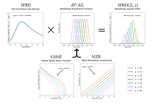
Figure 2: Schematic depiction of how our model for the metallicity specific star formation rate density, SFRD$(Z_{\rm{i}},z)$, is created from multiplying a star formation rate density (SFRD) with a metallicity probability distribution function, $\mathop{}\!\mathrm{d}P/\mathop{}\!\mathrm{d}Z_{\rm{i}}$. The metallicity distribution function is constructed by convolving a galaxy stellar mass function with a mass-metallicity relationship. An exception is our fiducial SFRD$(Z_{\rm{i}},z)$ model, which uses the ‘preferred’ phenomenological model from Neijssel et al. (2019) for the metallicity distribution function. The arrows in each sub-figure indicate in which direction the distribution moves as redshift increases.

$$\mathcal{R}_{\rm{m}}({t}_{\rm{m}},m_{1,\rm{f}},m_{2,\rm{f}})=\frac{\mathop{}\!\mathrm{d}^{4}{N}_{\rm{merger}}}{\mathop{}\!\mathrm{d}{t}_{\rm{s}}\mathop{}\!\mathrm{d}{V}_{\rm{c}}\mathop{}\!\mathrm{d}m_{1,\rm{f}}\mathop{}\!\mathrm{d}m_{2,\rm{f}}}({t}_{\rm{m}},m_{1,\rm{f}},m_{2,\rm{f}})$$

$$=\int\mathop{}\!\mathrm{d}Z_{\rm{i}}\int_{0}^{{t}_{\rm{m}}}\mathop{}\!\mathrm{d}{t}_{\rm{delay}}\,{\rm{SFRD}}(Z_{\rm{i}},{t}_{\rm{form}}={t}_{\rm{m}}-{t}_{\rm{delay}})\,\times$$

$$\,\hskip 85.35826pt\mathcal{R}_{\rm{form}}(Z_{\rm{i}},{t}_{\rm{delay}},m_{1,\rm{f}},m_{2,\rm{f}}),$$ (2)

where ${t}_{\rm{s}}$ is the time in the source frame of the merger, ${V}_{\rm{c}}$ is the comoving volume, $\mathcal{R}_{\rm{form}}$ is obtained using COMPAS (Section 2.2) and ${\rm{SFRD}}(Z_{\rm{i}},{t}_{\rm{form}})={\rm{SFRD}}(Z_{\rm{i}},z({t}_{\rm{form}}))$. We obtain the SFRD$(Z_{\rm{i}},z)$ by multiplying a SFRD with a metallicity probability density function

$${\rm{SFRD}}(Z_{\rm{i}},z_{\rm{form}})=\frac{\mathop{}\!\mathrm{d}^{3}{M}_{\rm{SFR}}}{\mathop{}\!\mathrm{d}{t}_{\rm{s}}\mathop{}\!\mathrm{d}{V}_{\rm{c}}\mathop{}\!\mathrm{d}Z_{\rm{i}}}(z_{\rm{form}})$$

$$=\underbrace{\frac{\mathop{}\!\mathrm{d}^{2}{M}_{\rm{SFR}}}{\mathop{}\!\mathrm{d}{t}_{\rm{s}}\mathop{}\!\mathrm{d}{V}_{\rm{c}}}(z_{\rm{form}})}_{\text{SFRD}}\times\underbrace{\frac{\mathop{}\!\mathrm{d}P}{\mathop{}\!\mathrm{d}Z_{\rm{i}}}(z_{\rm{form}})}_{\text{GSMF $+$ MZR}},$$ (3)

where we wrote down the equations in $z$, and used the short hand notation $z_{\rm{form}}=z({t}_{\rm{form}})$. We use for the metallicity density function, ${\mathop{}\!\mathrm{d}P}/{\mathop{}\!\mathrm{d}Z_{\rm{i}}}$, either a direct analytical formula (e.g. model $\mu=000$), or, in most cases, a convolution between a galaxy mass function, the number density of galaxies per logarithmic mass bin (GSMF) and mass-metallicity relation (MZR). This is discussed in more detail below and schematically shown in Figure 2. Throughout our analysis we use the cosmology parameters from the WMAP9 study (Hinshaw et al., 2013).

This merger rate density, $\mathcal{R}_{\rm{m}}$, is then converted to a local detection rate by integrating over the co-moving volume and taking into account the probability, ${P}_{\rm{det}}$, of detecting a GW source (Section 2.5) with

$$\mathcal{R}_{\rm{det}}({t}_{\rm{det}},m_{1,\rm{f}},m_{2,\rm{f}})=\frac{\mathop{}\!\mathrm{d}^{3}{N}_{\rm{det}}}{\mathop{}\!\mathrm{d}{t}_{\rm{det}}\mathop{}\!\mathrm{d}m_{1,\rm{f}}\mathop{}\!\mathrm{d}m_{2,\rm{f}}}$$

$$=\int\mathop{}\!\mathrm{d}{V}_{\rm{c}}\,\frac{\mathop{}\!\mathrm{d}{t}_{\rm{s}}}{\mathop{}\!\mathrm{d}{t}_{\rm{det}}}\,\mathcal{R}_{\rm{m}}({t}_{\rm{m}},m_{1,\rm{f}},m_{2,\rm{f}})\,{P}_{\rm{det}}(m_{1,\rm{f}},m_{2,\rm{f}},{D}_{\rm{L}}(z)),$$ (4)

where ${t}_{\rm{det}}$ is the time in the detector (i.e., the observer) frame and ${D}_{\rm{L}}$ is the luminosity distance. See Appendix A for more details about the conversion to ${t}_{\rm{det}}$, $z$ and ${D}_{\rm{L}}$. In practise we often marginalize in the remaining sections over the masses and redshifts (or equivalent, delay or merger time) to obtain an overall rate in this Equation as well as Equation 1. We also calculate the detector rate for where ${t}_{\rm{det}}$ is the current age of our Universe.

In practice, the integral in Equation 2.3 is estimated using a Riemann sum over redshift, metallicities and delay time bins, given in Equation 9. This method is similar to previous work including Dominik et al. (2013, 2015); Belczynski et al. (2016b); Mandel & de Mink (2016); Barrett et al. (2018); Eldridge et al. (2019); Baibhav et al. (2019); Bavera et al. (2020) and Chruslinska et al. (2019). Details of our method are given in Neijssel et al. (2019) and C21.

xyz index	SFRD [x]	GSMF [y]	MZR [z]
000 (fiducial)	phenomenological model Neijssel et al. (2019)
1	Madau & Dickinson (2014)	Panter et al. (2004)	Langer & Norman (2006)
2	Strolger et al. (2004)	Furlong et al. (2015) single Schechter	Langer & Norman (2006) $+$ offset
3	Madau & Fragos (2017)	Furlong et al. (2015) double Schechter	Ma et al. (2016)

Table 3: List of the assumptions for the metallicity-specific star formation rate, SFRD$(Z_{\rm{i}},z)$, models that we explore in this study. All SFRD$(Z_{\rm{i}},z)$ models except our fiducial model are obtained by combining a star formation rate density (SFRD) with a galaxy stellar mass function (GSMF) and mass-metallicity relation (MZR). See Sections 2.3 and 2.4 for more details. The models are named in the convention $\rm{xyz}$ with $\rm{x,y,z}\in[1,2,3]$ the index numbers for the models used for the SFRD, GSMF and MZR, respectively. For example, the combination of using the Madau & Dickinson (2014) SFRD with the Panter et al. (2004) GSMF and Ma et al. (2016) MZR is labeled ${113}$. The fiducial (phenomenological) model is not a specific combination but a parameterized model that is built to be flexible and is fitted to match the GW detected BHBH rate and chirp mass distribution from the first two runs of LIGO and Virgo (Neijssel et al., 2019). The simulations using the phenomenological SFRD$(Z_{\rm{i}},z)$ model have the label ${000}$

2.4 Metallicity-specific star formation rate density prescriptions

We explore the impact on the BHNS merger rate and population characteristics from a total of $28$ different SFRD$(Z_{\rm{i}},z)$ models. All our $28$ SFRD$(Z_{\rm{i}},z)$ models are constructed by combining analytical, simplified, prescriptions for the star formation rate density and metallicity distribution function (Equation 3). A schematic depiction is shown in Figure 2. Although all models (drastically) simplify the complex behavior of the SFRD$(Z_{\rm{i}},z)$ as a function of redshift and time, many of the prescriptions explored in this work are widely used in population synthesis predictions for DCO mergers. Our aim in using these models is foremost to explore and study the impact of these uncertainties in current state-of-the-art population synthesis predictions for BHNS mergers. In Section 5.1.3 we discuss in more detail the main limitations and future prospects to this modelling.

Our fiducial SFRD$(Z_{\rm{i}},z)$ model, $\rm{xyz}={{000}}$ (Table 3), is the phenomenological model described in Neijssel et al. (2019) (refered to as the ‘preferred’ model). This model uses a phenomenological analytical model for the SFRD and the metallicity probability distribution function. The latter is directly constructed using a log-normal metallicity density distribution with a redshift independent standard deviation $\sigma=0.39$ and redshift dependent mean $\mu(z)$, which follows the work of Langer & Norman (2006). The values of the free parameters in the phenomenological model are found by combining the SFRD$(Z_{\rm{i}},z)$ prescription with a population synthesis outcome to find the best fit to the BHBH GW observations announced in the first two observing runs of LIGO and Virgo (Neijssel et al., 2019). This work is also done with COMPAS using stellar-evolution assumptions that are similar to the ones assumed in this study. We therefore expect the merger rates based on this SFRD$(Z_{\rm{i}},z)$ choice and our fiducial simulations to be representative for the GW observations. The SFRD and metallicity probability distribution function for this prescription are shown in Figure LABEL:fig:MSSFR-SFRs and LABEL:fig:MSSFR-Z-PDFs, respectively.

All our other 27 SFRD$(Z_{\rm{i}},z)$ models, on the other hand, use one of the commonly used SFRDs in combination with a probability density function that is created by combining a GSMF with a MZR, these are described below. The main difference of these models compared to the preferred Neijssel et al. (2019) model is that the former does not assumes the metallicity probability distributions are symmetric in log-metallicity (whilst the preferred model from Neijssel et al. 2019 does), as can be seen in Figure LABEL:fig:MSSFR-Z-PDFs. Observational evidence suggests this symmetric behavior is likely not the case (e.g. Langer & Norman, 2006; Chruslinska et al., 2019; Boco et al., 2021). Two combinations of the 27 SFRD$(Z_{\rm{i}},z)$ models are shown in Figure LABEL:fig:MSSFR-Z-PDFs. By considering all possible combinations of the three SFRD, three GSMF and three MZR prescriptions, we end up with a total of 27 SFRD$(Z_{\rm{i}},z)$ models in addition to our fiducial SFRD$(Z_{\rm{i}},z)$ model based on Neijssel et al. (2019), resulting in a total of $28$ models.

2.4.1 Star formation rate density SFRD

The SFRDs prescriptions are shown in Figure LABEL:fig:MSSFR-SFRs. Besides using the phenomenological SFRD from Neijssel et al. (2019) for model 000, we follow Neijssel et al. (2019) and vary between three typically used SFRD prescriptions described in Table 3. First, we use the SFRD from Madau & Dickinson (2014, Equation 15), which has a slightly earlier peak compared to the other SFRDs used in this work. Population synthesis studies of DCO merger rates that use this SFRD prescription include Belczynski et al. (2016a); Chruslinska et al. (2018); Baibhav et al. (2019) and Eldridge et al. (2019). Secondly, we use the Strolger et al. (2004) prescription, which assumes a higher extinction correction, resulting in a higher SFRD, particularly at higher redshifts. Population synthesis studies of DCO merger rates that use this SFRD prescription include the work by Dominik et al. (2013); Kowalska-Leszczynska et al. (2015); Belczynski et al. (2017); Cao et al. (2018) and Kruckow et al. (2018). Last, we also use the SFRD from Madau & Fragos (2017, Equation 1), which is an updated version of Madau & Dickinson (2014) that uses the broken power law initial mass function from Kroupa (2001) and better fits some of the observations between redshifts $4\lesssim z\lesssim 10$. DCO merger rate studies that use this SFRD assumption include Belczynski et al. (2020); Drozda et al. (2020); Wong et al. (2021) and Zevin et al. (2020a).

2.4.2 Galaxy stellar mass function GSMF

Following Neijssel et al. (2019), we vary between three different prescriptions for the GSMF, which are shown in Figure LABEL:fig:MSSFR-GSMFs. Typically, the GSMF is described with a single or double Schechter (1976) function. First, we use a redshift independent single Schechter GSMF model as given by Panter et al. (2004). This GSMF prescription is used to create a metallicity distribution function by Langer & Norman (2006), which is used by studies including Barrett et al. (2018) and Marchant et al. (2017). Second and third we use the redshift dependent single and double Schechter functions based on results from Furlong et al. (2015), respectively. We use the fits by Neijssel et al. (2019) to the tabulated values from Furlong et al. (2015, table A1), that extrapolates to a full redshift range of $z\in[0,6.5]$. See Neijssel et al. (2019) for more details.

2.4.3 Mass-metallicity relation MZR

We follow Neijssel et al. (2019) for exploring three different MZR prescriptions shown in Figure LABEL:fig:MSSFR-MZRs. The metallicity in this figure is shown as the number density of oxygen over that of hydrogen, which is typically observed. The MZR describes the average relation between the typical metallicities found for star forming galaxies at a given redshift. We use the solar values of $\,\rm{Z}_{\odot}=0.0142$ and $\log_{10}[\rm{O}/\rm{H}]+12=8.69$ (Asplund et al., 2009) to convert to mass fraction metallicities. For our first two MZR prescriptions we use the approximate MZR relation that Langer & Norman (2006) construct based on observations from Savaglio et al. (2005), which is given by $M_{*}/M_{x}=(Z_{\rm{i}}/Z_{\odot})^{2}$, with $M_{x}$ as given by Langer & Norman (2006) and $M_{*}$ the galaxy stellar mass. We assume the average metallicity scales with redshift as $\langle Z_{\rm{i}}\rangle=Z_{\odot}10^{-0.3z}$. Following Neijssel et al. (2019) we create a second prescription based on these two relations, by adding an offset to better match the quadratic fit given in Savaglio et al. (2005). As third MZR model we use the MZR relation given by Ma et al. (2016). See Neijssel et al. (2019) for more details. We do not take into account the observed scatter around the MZR, see for more details (Chruslinska & Nelemans, 2019).

2.5 Detection probability of a source

Whether a BHNS merger is detectable by a GW interferometer network depends on its distance, orientation, inclination and source characteristics (such as component masses $m_{1,\rm{f}}$, $m_{2,\rm{f}}$). The detectability is described by a source signal-to-noise ratio (SNR). We follow the method from Barrett et al. (2018) to calculate the probability of detecting GW sources. We assume a SNR threshold of $8$ for a single detector (Finn & Chernoff, 1993) as a proxy for detectability by the network. The SNR of the BHNS mergers are calculated by computing the source waveforms using a combination of the LAL suite software packages IMRPhenomPv2 (Hannam et al., 2014; Husa et al., 2016; Khan et al., 2016) and SEOBNRv3 (Pan et al., 2014; Babak et al., 2017). We marginalize over the sky localization and source orientation of the binary using the antenna pattern function from Finn & Chernoff (1993). The detector sensitivity is assumed to be equal to advanced LIGO in its design configuration (LIGO Scientific Collaboration et al., 2015; Abbott et al., 2016, 2018a), which is equal to that of a ground-based GW detector network composed of Advanced LIGO, Advanced Virgo and KAGRA (LVK). We ignore the effect of the BH spin orientation and magnitude on the detectability of GWs, which is expected to possibly increase detection rates within a factor 1.5 (Gerosa et al., 2018) as binaries with (high) aligned spins are predicted to have larger horizon distances (Campanelli et al., 2006; Scheel et al., 2015).

2.6 Tidally disrupted BHNS

Simulations show that during a BHNS merger the NS is either tidally disrupted outside of the BH innermost stable circular orbit or instead plunges in, depending on the mass ratio, BH spin and NS equation of state (Pannarale et al., 2011; Foucart, 2012; Foucart et al., 2018). If the NS is disrupted, part of the disrupted material can form a disk and can eventually power electromagnetic counterparts such as short gamma-ray bursts and kilonovae (Bhattacharya et al., 2019; Barbieri et al., 2020; Zhu et al., 2020). We estimate the ejected mass during a BHNS merger using Equation 4 from Foucart et al. (2018) who present a simple formula for the merger outcome, post-merger remnant mass and ejecta mass based on numerical relativity simulations. We define a BHNS merger to ‘disrupt’ the NS if the calculated ejecta mass is nonzero. By doing so, we can calculate the fraction of BHNS mergers that disrupt the NS outside of the BH innermost-stable orbit, which are interesting candidates for observing an electromagnetic counterpart to their GW detection. Detecting BHNS mergers with electromagnetic counterparts is a golden grail in astronomy as it would confirm the origin of such transients and enables, e.g. measurements of the NS equation of state and BHNS system. There has been a big effort in finding such a counterpart, such as to the possible BHNS merger GW190814, but so far without a detection (e.g. Gomez et al., 2019; Dobie et al., 2019; Ackley et al., 2020).

As the NS equation of state is unknown we explore two variations for the NS radius: we assume ${R}_{\rm{NS}}=11.5$$\,\rm{km}$ or ${R}_{\rm{NS}}=13$$\,\rm{km}$ consistent with the APR equation of state (Akmal et al., 1998) and GW observations (Abbott et al., 2018b), and the NICER observations (e.g. Miller et al., 2019), respectively.

The spins of the BHs in BHNS mergers, ${\chi}_{\rm{BH}}$, are also unknown (e.g. Miller & Miller, 2015). For the BH spin we explore three models. First, we assume all black holes to have zero spin, ${\chi}_{\rm{BH}}=0$. Second, we assume all BHs to have half the maximum spin value, ${\chi}_{\rm{BH}}=0.5$, which explores a scenario where BHs in BHNS have more moderate spins. Last, we explore an ad hoc, but physically motivated spin model where we assign spins based on the study by Qin et al. (2018). Here it is assumed that all first formed BHs in BHNS binaries have zero spin as a consequence of efficient angular momentum transport (Fragos & McClintock, 2015; Qin et al., 2018; Fuller & Ma, 2019; Belczynski et al., 2020). The helium star progenitors of BHs that form second in the binary, however, can spin up through tidal interactions if they are in a close orbit with their companion, leading to BHs with significant spins (cf. van den Heuvel & Yoon, 2007; Kushnir et al., 2016; Qin et al., 2018; Bavera et al., 2020; Mandel & Fragos, 2020). For these NS–BH binaries, we use an approximate prescription to determine the BH spin:

$$\chi_{\mathrm{BH}}=\begin{cases}0&\text{for }\log_{10}(P)>0.3\\ 1&\text{for }\log_{10}(P)<-0.3\\ -5/3\log_{10}(P)+0.5&\text{for }-0.3<\log_{10}(P)<0.3,\end{cases}$$ (5)

where $P$ is the orbital period of the binary in days right before the second SN. We follow with this the prescription in Chattopadhyay et al. (2021), who create this ad hoc fit from the top middle panel of Figure 6 in Qin et al. (2018), which is based on a simulation for solar metallicity. Although in reality the spin distribution is more complicated and metallicity dependent, we use this single prescription for simplification. We expect that this does not impact drastically our results as the variation over metallicity are minor compared to the overall behavior of most BHs having zero spin, and only close NS–BH binaries having high spins. Moreover, we show in Section 4.1.5 that the amount of systems with ejecta is in this prescription dominated by the number of NS–BH binaries, and as this fraction is low, that this prescription is most similar to the assumption where all ${\chi}_{\rm{BH}}$ are zero.

We assume the BH spin to be aligned with the orbit and not vary from the moment the BHNS has formed. For each spin model, we vary the two NS radii assumptions, resulting in six different combinations of BH spin and NS radius. See Zappa et al. (2019) and Zhu et al. (2020) for a further discussion on the effect of different equations of state and BH spins on BHNS ejecta.

2.7 Statistical sampling uncertainty

Each of our simulations yield a finite number of BHNS mergers, as quoted in the last column of Table 2, which results in a statistical sampling uncertainty. We calculated this uncertainty on the BHNS formation rate (Equation 1) using Equation 15 from Broekgaarden et al. (2019) and found that this statistical uncertainty is at most $0.06\%$, less than a tenth of a percent. This is negligible compared to the systematic uncertainties from our assumptions in modelling of the massive binary evolution and the SFRD$(Z_{\rm{i}},z)$ . We therefore decide to not quote these statistical sampling uncertainties throughout the remaining of the paper, and instead focus on the uncertainty from stellar evolution and SFRD$(Z_{\rm{i}},z)$ variations. An interested reader can find more details on the statistical uncertainties in the related script in https://github.com/FloorBroekgaarden/BlackHole-NeutronStar and in Broekgaarden et al. (2019) and references therein.

3 Fiducial model

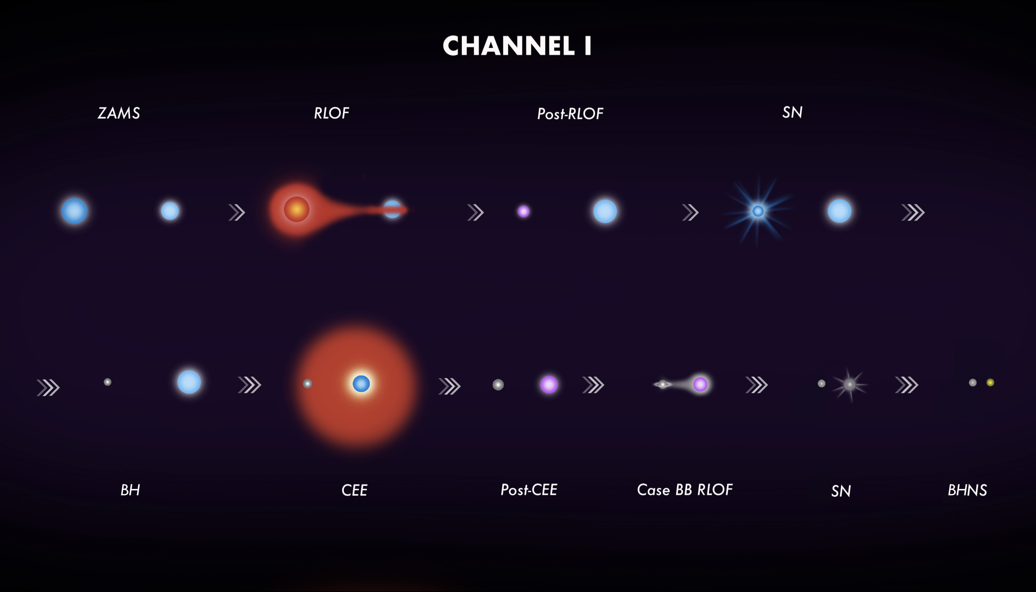
Figure 3: Schematic depiction of the classic formation channel as described in Section 3.1.1. The acronyms stand for: zero-age main sequence (ZAMS), Roche lobe overflow (RLOF), supernova (SN), black hole (BH), common-envelope episode (CEE), and black hole-neutron star (BHNS). The figure is based on Figure 1 from Vigna-Gómez et al. (2020) by T. Rebagliato, which is publicly available at https://zenodo.org/record/3634498#.XnS9ZC2ZNQI. Adjustments to the original image were made by S. Vinciguerra.

In this section we describe the results of our population synthesis simulation for model $\rm{A}000$, which uses both our fiducial assumptions for the massive (binary) star model (described in Section 2.1 and listed in Table 1) and our fiducial assumptions for the cosmic star formation history model (described in Section 2.4 and listed in Table 3). We focus on this model to provide insight to a typical output of a COMPAS simulation. This model choice is similar to earlier work done with COMPAS and has been chosen as it, for example, matches the population of galactic NSNS systems (Vigna-Gómez et al., 2018; Chattopadhyay et al., 2020) and the rate and chirp mass distributions of the GW sources in the first two observing runs of LIGO and Virgo (Neijssel et al., 2019). In Section 4 we describe the results for all $420$ model variations.

3.1 Formation channels

We identify four main groups of formation channels described below. The percentages, quoted after each section header, indicate the fraction that each channel contributes to the total number of detected BHNS mergers. This takes into account the SFRD$(Z_{\rm{i}},z)$ weighting using our fiducial model ($\rm{xyz}=000$) and the detection probability of a GW network equivalent to LVK at design sensitivity. These percentages are calculated using Equation 2.3, whilst marginalizing over the BHNS masses. The percentage that each formation channel contributes to the detectable merger rate is impacted by variations in the population synthesis and SFRD$(Z_{\rm{i}},z)$ models. We present results for our $420$ models in Section 4.1.3.

3.1.1 (I) Classic channel $86\%$

We find, in agreement with, e.g. Neijssel et al. (2019) for BHBH mergers, that the majority of the binaries form a BHNS through the ‘classic’ formation channel where the binary experiences both a stable mass transfer and an unstable (CE) mass transfer phase. This classic channel is discussed in e.g. Bhattacharya & van den Heuvel (1991); van den Heuvel & De Loore (1973); Tauris & van den Heuvel (2006) and Belczynski et al. (2008), see also Mandel & Farmer 2018 and references therein. We schematically depict this formation channel in Figure 3 and describe it below in more detail for binaries that form a BHNS merger.

The binaries in the classic channel are born with a wide range of initial separations of about $0.3$–$20$$\,\mathrm{AU}$ as shown in Figure 4. The initially more massive star (the primary) eventually expands and fills its Roche lobe initiating a stable mass transfer phase (Roche-lobe overflow, RLOF) onto the initially less massive star (the secondary). This happens in this channel either when the primary is a Hertzsprung gap star or is a core helium burning star (both case B mass transfer), where core helium burning donor stars are in initially wider binaries compared to Hertzsprung gap donor stars. In our fiducial model the companion typically accretes a large fraction of the mass that is lost from the primary star donor. Mass transfer typically ends in our simulations when the donor has lost all of its hydrogen envelope. The result for case A or B mass transfer is typically a stripped envelope star that is burning helium, which may be observed as a Wolf-Rayet star (e.g. Crowther, 2007; Götberg et al., 2018).

Eventually, the stripped primary star ends its life in a core-collapse (SN) and the first compact object, a BH or NS, is formed. The binary needs to stay bound during the SN to eventually form a BHNS. Typically, more than 80$\%$ of the binaries disrupt during the first SN (e.g. Renzo et al., 2019), where disruption depends on the magnitude and orientation of the SN kick, the separation of the binary and the amount of ejected mass (e.g. Flannery & van den Heuvel 1975; Tauris & Takens 1998).

The secondary star later evolves off the main sequence, and expands to fill its Roche lobe. This is the start of a reverse mass-transfer phase from the secondary onto the compact object. However, for this reverse mass-transfer phase the extreme mass ratio contributes to the mass transfer being dynamically unstable, and the start of CE evolution (e.g. Soberman et al., 1997; Ge et al., 2010; Ge et al., 2015; Vigna-Gómez et al., 2018). During the CE event the separation of the binary decreases as orbital angular momentum and energy are transferred to the CE. If the CE is ejected successfully, the result is a close binary system consisting of a BH or NS and a massive helium star, an example of a possible observed system in this phase is Cyg X-3 (Belczynski et al., 2013; Zdziarski et al., 2013). Otherwise the system results in a merger of the star with the compact object, which can possibly form a Thorne–Żytkow object (Thorne & Zytkow, 1977) or lead to peculiar SNe (e.g. Chevalier, 2012; Pejcha et al., 2016; Schrøder et al., 2020).

In a subset of the binaries there is a stable case BB mass transfer phase after the CE from the helium star onto the primary compact object (cf. Dewi & Pols, 2003). This typically occurs when the secondary is a relatively low mass helium star as they expand to larger radii compared to more massive helium stars in the single star prescriptions of Hurley et al. (2000) implemented in COMPAS (cf. Dewi & Pols, 2003). However, Laplace et al. (2020) point out that these prescriptions might underestimate the expansion of helium stars, especially at metallicities $Z_{\rm{i}}\approx 0.001$. BHNS systems undergoing case BB mass transfer typically have the shortest semi-major axis in Figure 6.

The helium star eventually forms a NS or BH in the second SN. If the binary remains bound, a BHNS binary is formed with masses as in Figure 6 that gradually decays in separation due to the emission of GWs. If the separation is small enough (typically $\lesssim 10$$\,\rm{R}_{\odot}$, see Figure 6) the BHNS will merge within ${t}_{\mathcal{H}}$.

3.1.2 (II) Only stable mass transfer channel $4\%$

In about $4\%$ of all detectable mergers the binary forms similar to the classic channel (I) but does not experience an unstable mass transfer phase leading to a CE. This channel thus only has stable mass transfer phases (cf. van den Heuvel et al. 2017; Neijssel et al. 2019, see also, e.g. Pavlovskii et al. 2017). To form BHNS systems with semi-major axis $\lesssim 10$$\,\rm{R}_{\odot}$ that can merge in ${t}_{\mathcal{H}}$, these binaries typically experience a second stable mass transfer phase from the secondary star onto the compact object after the first SN that decreases the separation of the binary. This formation channel typically leads to BHNS mergers with final mass ratios $q_{\rm{f}}\equiv m_{\rm{BH}}/m_{\rm{NS}}\approx 3$ as shown in Figure 6 and 8.

3.1.3 (III) Single-core CE as first mass transfer channel $4\%$

In the window of initial separations between $\sim 5$–$40$$\,\mathrm{AU}$ as shown in Figure 4, the first mass transfer phase leads to an unstable single-core CE event, with only the donor star having a clear core-envelope structure and the secondary star still being a main sequence star. This is in agreement with other studies on mass transfer stability (see e.g. Figure 19 and 20 in Schneider et al., 2015). The donor star that initialized the CE is typically a core helium burning star or a star on the giant branch. If the CE is successfully ejected this leads to a tight binary star system. The primary star will eventually form a BH in a SN. Eventually the secondary star also evolves off the main sequence, leading to either a stable mass transfer phase or a second unstable CE event. The latter occurs for the widest binaries in Figure 4. The secondary eventually forms a NS. In this formation channel the BH always forms first in our simulations. This formation channel typically leads to BHNS mergers with final BHNS mass ratios $q_{\rm{f}}\approx 3$ as shown in Figure 6 and 8.

3.1.4 (IV) Double-core CE as first mass transfer channel $<1\%$

In this channel the primary star fills its Roche lobe when both stars are on the giant branch and both stars have a core-envelope structure. The mass transfer is unstable, leading to a double-core CE. Both stars need to evolve on a similar timescale and, therefore, have similar initial masses (i.e., $0.9\lesssim q_{\rm{i}}\lesssim 1$) as can be seen in the bottom panel of Figure 4. The further evolution of the binary proceeds similar to channel III, except that in most cases there is never a case BB mass transfer phase. A BHNS system can be formed if the stars have carbon-oxygen core masses close to the boundary between NS and BH formation in our remnant mass prescription. This is visible in Figure 6 where it can be seen that the BHNS in this channel have BH and NS masses that are very equal compared to the other formation channels. This formation channel typically also leads to BHNS mergers with the smallest final mass ratios $q_{\rm{f}}\approx 1.5$ as shown in Figure 6 and 8. These low BHNS masses cause GW detectors to be less sensitive to finding binaries from this channel. This results in $<1\%$ of the detections being predicted from this channel. Which is different from the expected contribution of this channel to e.g. binary neutron star mergers (Vigna-Gómez et al., 2018) This channel is similar to the one described by Brown (1995); Bethe & Brown (1998) and later on by, e.g. Dewi et al. (2006); Justham et al. (2011) and Vigna-Gómez et al. (2018).

3.1.5 (V) Other channel $6\%$

We classify all other BHNS under the ‘other’ channel. The majority of contributions comes from two formation pathways. First, a large fraction of the other channel consists of binaries born with low metallicities and initial separations between about $0.01$–$0.20$$\,\mathrm{AU}$ (gray scatter points in bottom right of the bottom left panel of Figure 6). These binaries undergo mass transfer when the donor star is a main sequence star (case A), which typically results in the secondary star accreting a large amount of mass from the primary. A lot of binaries from this formation pathway form the NS first. Second, most of the remaining binaries in the ‘other’ channel form by having a ‘lucky SN natal kick’. The first event in this pathway is the primary star undergoing a SN, and in a tiny fraction of those binaries the natal kick has the right magnitude and direction so that the binary stays bound.

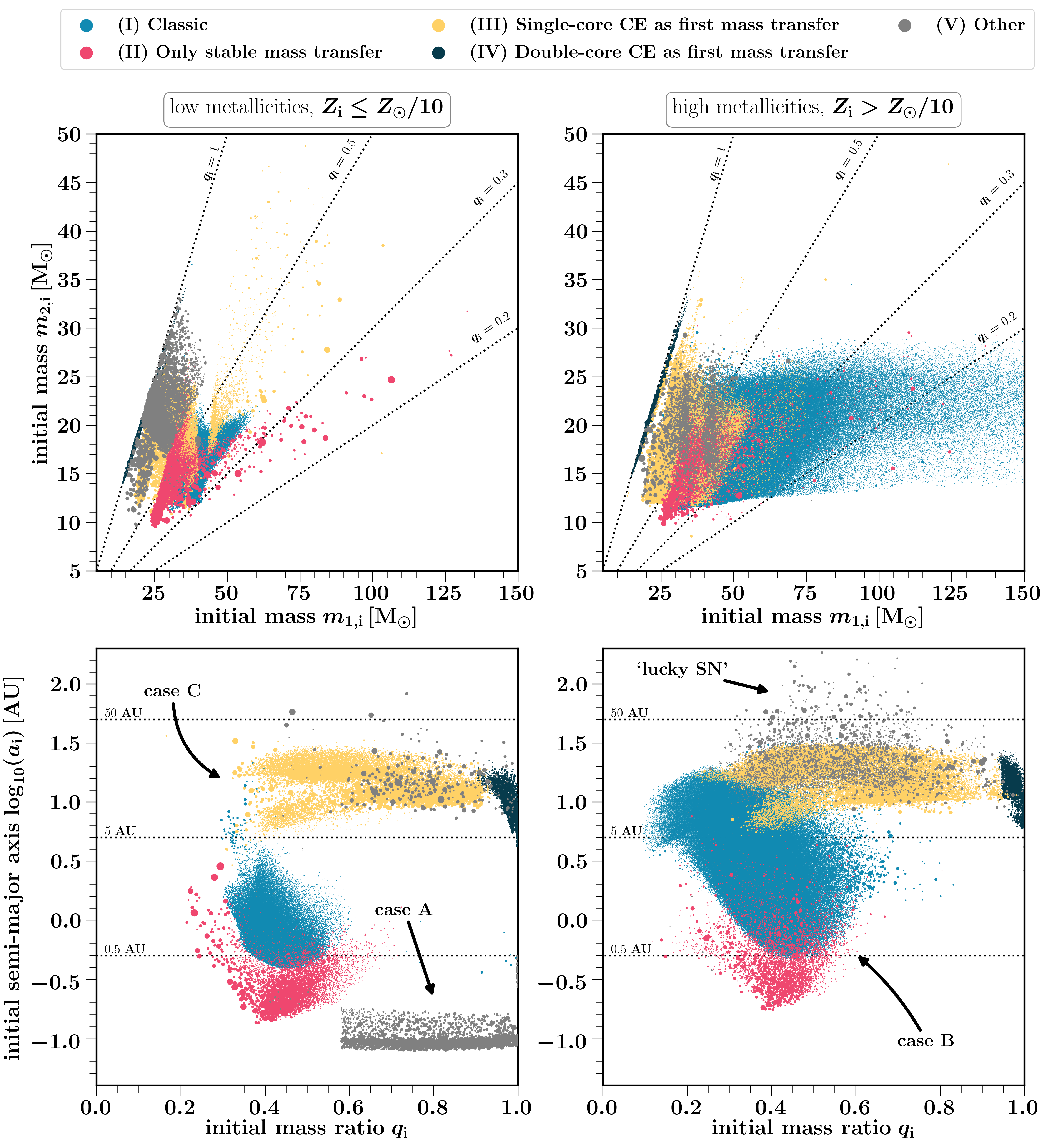
Figure 4: Initial parameters of binaries forming BHNS systems that merge in ${t}_{\mathcal{H}}$ for our fiducial model $\rm{A}000$ (Section 2) for ‘lower’ metallicities $Z_{\rm{i}}\leq\,\rm{Z}_{\odot}/10$ (left panels) and ‘higher’ metallicities $Z_{\rm{i}}>\,\rm{Z}_{\odot}/10$ (right panels), where $\,\rm{Z}_{\odot}=0.0142$. Colors represent different formation channels, described in Section 3.1. Each point represents one simulated binary system that leads to a BHNS merger. The areas of the points represent the statistical weight $w_{\rm{i}}$ (i.e., probability of occurrence) of that binary in our simulation. Dotted lines indicate some values of the parameters to guide the reader. We define the initial mass ratio $q_{\rm{i}}=m_{2,\rm{i}}/m_{1,\rm{i}}$. Arrows indicate regions where the first mass transfer is case A, B or C, as well as ‘lucky SN’ systems that do not experience mass transfer before the first SN. Figures and videos showing how these distributions change over our model variations are available at https://github.com/FloorBroekgaarden/BlackHole-NeutronStar.

3.2 Initial properties leading to BHNS mergers

The locations in the initial parameter space of the binaries (e.g. initial masses, initial mass ratio, and initial semi-major axis) leading to the formation of a BHNS system that merges in ${t}_{\mathcal{H}}$ are shown in Figure 4 for metallicities $Z_{\rm{i}}\leq\,\rm{Z}_{\odot}/10$ and $Z_{\rm{i}}>\,\rm{Z}_{\odot}/10$, which represent respectively lower and more solar like metallicity environments. We assume in our simulations $\,\rm{Z}_{\odot}=0.0142$ (Asplund et al., 2009). We chose the boundary $Z_{\rm{i}}=\,\rm{Z}_{\odot}/10$ somewhat arbitrarily as it is about half way in our $Z_{\rm{i}}$ grid (Figure 5).

3.2.1 Initial masses

As can be seen in the top panels of Figure 4, the majority of BHNS mergers at low $Z_{\rm{i}}$ originate from binaries with masses $10\lesssim$ $m_{1,\rm{i}}$/$\,\rm{M}_{\odot}$ $\lesssim 60$ and $10\lesssim$$m_{2,\rm{i}}$/$\,\rm{M}_{\odot}$ $\lesssim 30$, whilst at higher metallicities this shifts to $10\lesssim$ $m_{1,\rm{i}}$/$\,\rm{M}_{\odot}$ $\lesssim 150$ and $10\lesssim$$m_{2,\rm{i}}$/$\,\rm{M}_{\odot}$ $\lesssim 30$ respectively. A difference between the two panels is that, at higher metallicities, there are BHNS systems formed from binaries with initial mass ratios $\lesssim 0.3$, whereas these mostly lack at lower metallicities, as can also be seen in the lower panels of Figure 4. This is because higher metallicities correspond to stronger line-driven stellar winds, leading to more mass loss, which equalizes the more extreme mass ratio before the onset of mass transfer, making the mass transfer more stable and the system more likely to survive to form a GW progenitor (cf. Belczynski et al., 2010b; Giacobbo & Mapelli, 2018; Neijssel et al., 2019). At lower metallicities, there is fewer mass loss and so the mass ratio stays more extreme at the moment of mass transfer, making it often unstable and the stars merge. Moreover, on average the total initial mass of binaries is higher at higher metallicities, as at those metallicities stellar winds strip more mass from the system compared to lower metallicities (Belczynski et al., 2010b). This stripping leads to lower mass carbon-oxygen cores compared to those of stars born with the same masses at lower metallicities. So where at higher metallicities BHNS form, the same systems may form BHBH binaries at lower metallicities in our simulations.

3.2.2 Initial semi-major axis and mass ratio

The initial semi-major axis of the binaries forming BHNS mergers in Figure 4 spans the range of about $0.1\lesssim a_{\rm{i}}\lesssim 50$$\,\mathrm{AU}$ with higher metallicities favoring slightly larger $a_{\rm{i}}$. The latter seems counter-intuitive since stellar winds typically widen the binary, but comes from subtle and indirect effects of the wind loss being stronger at higher metallicities. As discussed above, the binaries at higher metallicities originate from initially more massive primary stars in the range $25$–$150$$\,\rm{M}_{\odot}$. The radii of these stars typically expand more during the Hertzsprung-gap phase in the stellar evolution tracks implemented in COMPAS (Hurley et al., 2000). Since this expansion, in combination with the initial separation, determines when mass transfer happens, the binary needs to have a much larger $a_{\rm{i}}$ at higher metallicities to form through the same channel as a binary at lower metallicities. In addition, the secondary star is typically more massive at the onset of a CE for higher metallicity binaries, causing the binary to shrink more compared to lower metallicity binaries (cf. Neijssel et al., 2019).

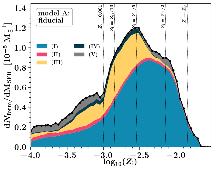
Figure 5: Number of BHNS mergers with ${t}_{\rm{delay}}\leq{t}_{\mathcal{H}}$ that form per unit star forming mass (${M}_{\rm{SFR}}$) as a function of initial metallicity $Z_{\rm{i}}$ for our fiducial model. This rate is obtained from Equation 1 by marginalizing over ${t}_{\rm{delay}}$, $m_{1,\rm{f}}$ and $m_{2,\rm{f}}$. The colors represent the contribution from each formation channel color coded as in Figure 4 and described in Section 3.1. The main formation channels are the (I) ‘classic’ channel (blue) and the (III) ‘single-core CE as first mass transfer channel’ (yellow). The 53 black scatter points denote the simulated $Z_{\rm{i}}$ grid points. Dotted lines indicate some $Z_{\rm{i}}$ values to guide the reader.

3.3 Yield of BHNS mergers as a function of birth metallicity

Figure 5 shows the contribution of the five formation channels to the yield of BHNS mergers as a function of metallicity. The yield of BHNS mergers peaks around metallicities $Z_{\rm{i}}\approx\,\rm{Z}_{\odot}/5$ ($Z_{\rm{i}}\approx 0.003$) and is lowest around $Z_{\rm{i}}\gtrsim\,\rm{Z}_{\odot}$, in broad agreement with e.g. Giacobbo & Mapelli (2018); Mapelli et al. (2019) and Neijssel et al. (2019), but there are some variations between these models in single stellar evolution, winds, mass transfer, and supernova prescriptions. The classic formation channel (channel I) dominates the yield. At metallicities $\log(Z_{\rm{i}})\lesssim\,\rm{Z}_{\odot}/2$ the other formation channels also contribute, particularly the single-core CE channel. For $Z_{\rm{i}}>\,\rm{Z}_{\odot}/2$ almost all BHNS mergers form through just two formation channels: the classic channel and a fraction forms through the only stable mass transfer channel. This is in agreement with Kruckow et al. (2018, see their Table C1) and is a result from a combination of the metallicity-dependent effects described in the paragraphs above.

That the BHNS yield peaks around $Z_{\rm{i}}\approx 0.003$ is due to line-driven stellar winds scaling positively with metallicity in our simulations (Section 2.1). First, at higher metallicities, higher wind-loss rates strip more mass from the star leading to lower compact object masses in our SSE and SN remnant prescription. Lower mass BHs receive larger natal kicks, have less mass fallback (leading to larger Blaauw kicks) and smaller total system masses making them more likely to disrupt during the SN. Second, at higher metallicities, binaries typically have wider separations after the second SN and therefore longer ${t}_{\rm{inspiral}}$ that may exceed ${t}_{\mathcal{H}}$. This is both because stellar winds widen the binary and because they result in stars with less massive envelopes, which reduces the amount of orbital hardening in mass transfer events (i.e., CE and stable Roche-lobe overflow). At metallicities $Z_{\rm{i}}\lesssim 0.001$, on the other hand, the formation rate of BHNS mergers is suppressed as the reduced stellar winds lead to massive enough carbon-oxygen cores that many systems instead form a BHBH merger. A second effect comes from that although overall the radius expansion of stars increases with increasing metallicity, particularly between $-3\lesssim\log(Z_{\rm{i}})\lesssim-2$ the radius extension of Hertzsprung-gap stars decreases for primary star masses that lie in the range to form BHNS mergers. This decrease in radial extension decreases the number of systems that merge as stars during mass transfer, (cf. Giacobbo & Mapelli, 2018), which increases the rate of BHNS formation.

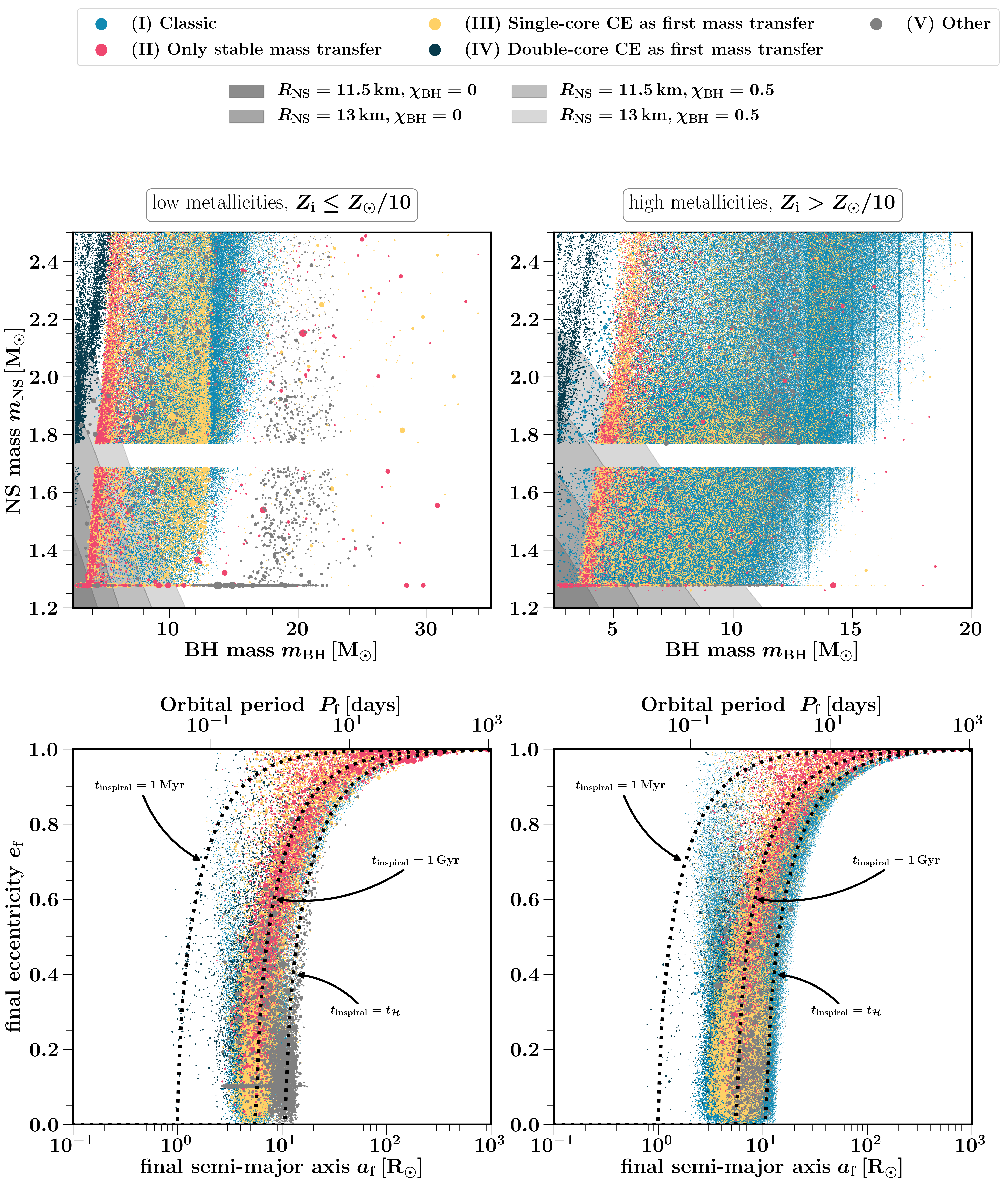
Figure 6: Same as Figure 5 for the BHNS properties at DCO formation, ${t}_{\rm{DCO}}$, for our Fiducial model $\rm{A}000$. The gray areas in the top panels denote the DCOs that have final masses such that the NS is tidally disrupted outside the BH innermost stable circular orbit based on Foucart et al. (2018) when assuming a NS radius ${R}_{\rm{NS}}\in\{11.5\,\rm{km},13\,\rm{km}\}$ and BH spins ${\chi}_{\rm{BH}}\in\{0,0.5\}$ for all BHs. Vertical lines, visible in the top right panel, are artificially caused by our model that maps for a specific $Z_{\rm{i}}$ a small range of stars with different initial masses to the exact same BH mass as described in Section 3.4.1. The dotted black lines in the bottom panels show lines of constant ${t}_{\rm{inspiral}}\in\{1\,\mathrm{Myr},1\,\mathrm{Gyr},{t}_{\mathcal{H}}\}$. For the orbital period on the second x-axis and the lines of constant inspiral time we assumed a fixed $m_{\rm{BH}}=10\,\rm{M}_{\odot}$ and $m_{\rm{NS}}=1.4\,\rm{M}_{\odot}$. Figures and videos showing how these distributions change over our model variations are available at %eccentricity␣␣versus␣semi-major␣axis␣of␣the␣\bhnsSingle␣binaries.https://github.com/FloorBroekgaarden/BlackHole-NeutronStar.

3.4 Final properties of BHNS mergers

The final characteristics of the BHNS systems at ${t}_{\rm{DCO}}$ (after the formation of the second compact object) are shown in Figure 6. In addition, Figure 7 shows the predicted distributions functions of the BHNS merger yield for five different simulated metallicities $Z_{\rm{i}}$ for typical BHNS characteristic at ${t}_{\rm{DCO}}$. These characteristics are the BH mass $m_{\rm{BH}}$, the NS mass $m_{\rm{NS}}$, mass ratio $q_{\rm{f}}=m_{\rm{BH}}/m_{\rm{NS}}$, eccentricity ${e}_{\rm{f}}$, total mass $m_{\rm{tot}}=m_{\rm{BH}}+m_{\rm{NS}}$, chirp mass ${\mathcal{M}}_{\rm{c}}$, which is a binary characteristic that is well measured by ground-based GW obervatories and is given by

$${\mathcal{M}}_{\rm{c}}=\frac{(m_{\rm{BH}}m_{\rm{NS}})^{3/5}}{(m_{\rm{BH}}+m_{\rm{NS}})^{1/5}},$$ (6)

the inspiral time ${t}_{\rm{inspiral}}$ and the semi-major axis, $a_{\rm{f}}$, at ${t}_{\rm{DCO}}$.

3.4.1 BH and NS remnant masses

The top panels in Figure 6 show that the simulated BHNS mergers have NSs with masses in the range $1.25\lesssim m_{\rm{NS}}/\,\rm{M}_{\odot}\leq 2.5$ (where the maximum NS mass is set to 2.5$\,\rm{M}_{\odot}$ in our fiducial model). The discontinuity in the NS remnant mass around 1.7$\,\rm{M}_{\odot}$ in Figure 6 and 7 results from the discontinuity in the proto-compact object mass equation at carbon-oxygen cores of $3.5$$\,\rm{M}_{\odot}$ in the delayed SN remnant mass prescription (Equation 18 in Fryer et al. 2012. The over-density of remnant masses around $1.3\,\rm{M}_{\odot}$ comes from two effects. First, the ECSN prescription map stars with different masses to a NS mass of 1.26$\,\rm{M}_{\odot}$, as described in Section 2.1 and Vigna-Gómez et al. (2018). Second, all NS progenitors with carbon-oxygen core masses below $2.5$$\,\rm{M}_{\odot}$ are in the delayed Fryer et al. 2012 remnant mass prescription mapped to NSs with with fixed masses $\approx 1.28\,\rm{M}_{\odot}$.

The majority of BHs in the BHNS binaries have masses in the range $2.5\leq m_{\rm{BH}}/\,\rm{M}_{\odot}\lesssim 20$, but this can extend to $m_{\rm{BH}}$ $\approx 30$$\,\rm{M}_{\odot}$ for very low values of $Z_{\rm{i}}$, as shown in the top left panel of Figure 6. We find that BHNS binaries with $m_{\rm{BH}}$ $\gtrsim 20$$\,\rm{M}_{\odot}$ are rare, in agreement with e.g. Rastello et al. (2020). At lower metallicities BHNS mergers are formed with more massive BHs compared to higher metallicities, as can be seen in the distributions of $m_{\rm{BH}}$, $q_{\rm{f}}$, $m_{\rm{tot}}$ and ${\mathcal{M}}_{\rm{c}}$ in Figure 7 that are more extended to higher masses for lower metallicities. This is because stars at lower metallicities lose less mass during their lives through line-driven stellar winds leading to larger remnant masses. The delayed SN remnant mass prescription does not lead to a BH mass gap between $2.5$–$5\,\rm{M}_{\odot}$ and we therefore find BHs with masses close to the maximum NS mass of $2.5\,\rm{M}_{\odot}$, as can be seen in Figures 6 and 7. The over-density in $m_{\rm{BH}}$ in straight vertical lines, particularly visible in the right top panel of Figure 6, is due to our prescription of LBV wind mass loss that maps a broad range of initial ZAMS masses to the same carbon-oxygen core masses and hence the same BH remnant masses (see for a discussion Appendix B of Neijssel et al. 2019). This results for some of our $Z_{\rm{i}}$ in peaks in the BH mass distribution around the highest BH mass for that metallicity as can be seen in the top right panel of Figure 6 and the top left panel of Figure 7.

A subset of the BHNS mergers in our fiducial simulation have final masses such that the NS is disrupted outside of the BH innermost stable circular orbit during the merger. This is shown in Figure 6 with the shaded areas for four different models for the NS radii and BH spins. Typically only the BHNS with low mass BHs and NS result in a tidal disruption of the NS. The fraction of BHNS mergers that disrupt the NS outside of the BH innermost stable orbit is strongly dependent on the assumed BH spin and NSs radii, with higher spins and larger NS radii leading to more tidally disrupted NSs. We discuss this in more detail in Section 3.5.7.

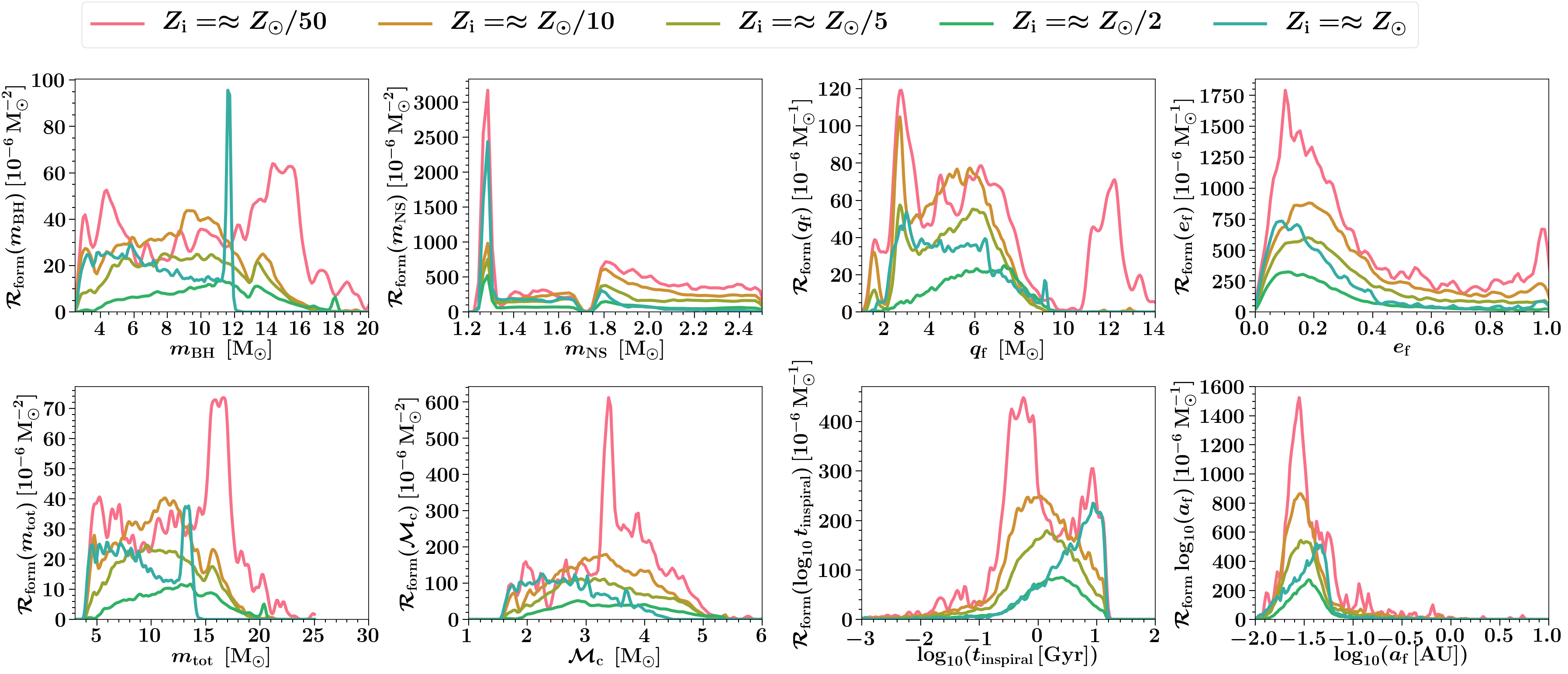
Figure 7: Distributions of the characteristics of BHNS systems that merge in ${t}_{\mathcal{H}}$ at ${t}_{\rm{DCO}}$ for five different metallicities $Z_{\rm{i}}$. The yield is calculated using Equation 1 and plotted using a weighted kernel density estimator with a dimensionless kernel bandwidth of 0.04, see the publicly available code for more details. We use the short hand notation $\mathcal{R}_{\rm{form}}(x)\equiv{\rm{d}}N/({\rm{d}}M_{\rm{SFR}}{\rm{d}}x)$ for variable $x$. The variables are described in Section 3.4. We warn the reader that interpertating the distributions of ${t}_{\rm{inspiral}}$ and $a_{\rm{f}}$ can be misleading as they are shown in log to best demonstrate the characteristics over the wide parameter range. Plots showing more intuitive (not log) distributions of ${t}_{\rm{inspiral}}$ and $a_{\rm{f}}$ are given in https://github.com/FloorBroekgaarden/BlackHole-NeutronStar.

3.4.2 Eccentricity and semi-major axis at ${t}_{\rm{DCO}}$

Figure 6 shows the semi-major axis and eccentricity for the BHNS mergers in our Fiducial model $\rm{A}000$. BHNS binaries that merge in ${t}_{\mathcal{H}}$ typically have merger times in the range $1\,\mathrm{Myr}\leq{t}_{\rm{inspiral}}\leq{t}_{\mathcal{H}}$ at the moment of the BHNS formation, corresponding to a semi-major axis between $1\lesssim a_{\rm{f}}/\,\rm{R}_{\odot}\lesssim 100$, as can be seen in the bottom panels of Figure 6. Systems with larger semi-major axis still merge in ${t}_{\mathcal{H}}$ if the binary is more eccentric as this decreases ${t}_{\rm{inspiral}}$. A subset of the binaries from the classic formation channel have the shortest semi-major axis at ${t}_{\rm{DCO}}$, which is because these system undergo a case BB mass transfer phase tightening the binary further after the CE phase.

Figure 6 shows that the BHNS eccentricities densely populate the full range 0–1, although smaller eccentricities are slightly favored as can be seen in Figure 7. We do not find clear subpopulations of BHNS systems with distinguishable eccentricity as discussed for NSNS systems by Andrews & Mandel (2019).

3.5 Predicted GW detectable BHNS distributions

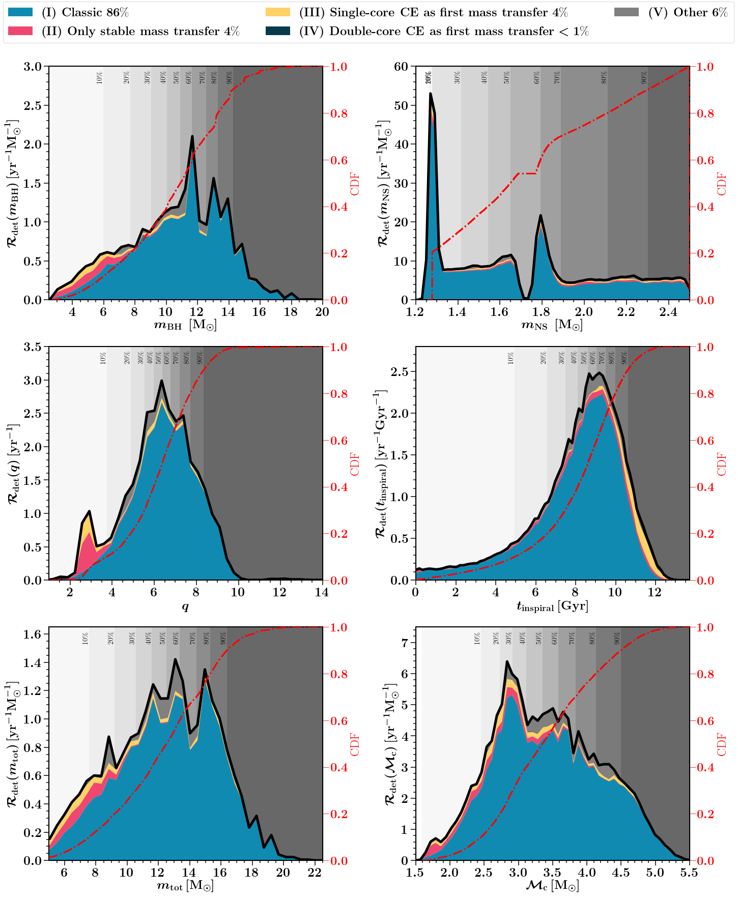
Figure 8: Predicted distributions of the detectable BHNS merger characteristics for our fiducial binary population synthesis and SFRD$(Z_{\rm{i}},z)$ model $\rm{A}000$ for a ground-based LVK detector network at design sensitivity. The detection rate is calculated using Equation 2.3. The colors in each graph, and the numbers quoted in the legend, represent the percentage that each formation channel (presented in Section 3.1) contributes to the total GW detected yield. The gap in the NS remnant mass distribution is caused by a discontinuity in the remnant mass prescription as discussed in Section 2.1. The red dashed-dotted lines show the cumulative distribution function (CDF). Gray areas indicate values for the CDF. The distributions are produced using a kernel density estimator with a bandwidth factor of 0.04, see our publicly available code for more details.

The predicted GW detectable BHNS distributions for a LVK network at design sensitivity are shown in Figure 8. We show the distribution for the BH mass, NS mass, mass ratio, inspiral times, total mass and chirp mass (Equation 6). Except for the inspiral times, ${t}_{\rm{inspiral}}$, all other BHNS parameters are typically obtained from GW observations (e.g. Abbott et al., 2017). The distributions and yields are determined using Equation 2.3, taking into account the SFRD$(Z_{\rm{i}},z)$ and detector probability (${P}_{\rm{det}}$) weighting. In this section we show the predicted distributions for our fiducial population synthesis and SFRD$(Z_{\rm{i}},z)$ model, given by $\rm{A}000$. In Section 4 we present the predicted BHNS distributions for all our $420$ model variations. The predicted distributions and characteristics for NSNS and BHBH mergers are given in a companion paper.

Our fiducial model $\rm{A}000$ presents an intrinsic BHNS merger rate at redshift zero of $\mathcal{R}_{\rm{m}}^{0}\approx 43$$\,\rm{Gpc}^{-3}$ $\,\rm{yr}^{-1}$ consistent with the inferred local BHNS merger rate density from Abbott et al. (2021d) of $\mathcal{R}_{\rm{m}}^{0}={45}_{-33}^{+75}$$\,\rm{Gpc}^{-3}$ $\,\rm{yr}^{-1}$ when assuming that GW200105 and GW200115 are representative of the entire BHNS population, whilst slightly below the inferred $\mathcal{R}_{\rm{m}}^{0}={130}_{-69}^{+112}$$\,\rm{Gpc}^{-3}$ $\,\rm{yr}^{-1}$ when Abbott et al. (2021d) assume a broader (and likely optimistic) distribution of component masses. When weighting for the sensitivity of a ground based GW network we find a detection rate of $\mathcal{R}_{\rm{det}}\approx 11$$\,\rm{yr}^{-1}$.

3.5.1 Formation channels

Our fiducial model predicts that about $86\%$ of the BHNS mergers detected by a LVK network at design sensitivity form through the classic formation channel (I, Section 3.1.1 and Figure 3). This percentage is higher compared to the average percentage that the classic channel contributes for each $Z_{\rm{i}}$ in our simulation (without the SFRD$(Z_{\rm{i}},z)$ and GW observation weighting). This results from two main effects. First, our fiducial SFRD$(Z_{\rm{i}},z)$ model convolved with the typical short delay times (Figure 7) for BHNS systems biases the detectable BHNS systems to originate from binary systems with initial metallicities $Z_{\rm{i}}\gtrsim\,\rm{Z}_{\odot}/2$. At these metallicities the contribution from other channels is relatively low (Figure 5). Second, the classic formation channel produces overall more massive BHNS systems compared to the other channels as shown in Figure 6, which are observed to larger distances with GW detectors. This further increases the contribution of the classic formation channel to eventually form the $86\%$.

The dominant channel for BHBH and NSNS observations is different compared to our findings for BHNS mergers. For BHBH mergers the majority of GW detected mergers are predicted to form through the only stable mass transfer channel (II, Neijssel et al., 2019, e.g.). For NSNS mergers about $60-70\%$ of the detected systems are predicted to form through the double-core CE channel (IV, Vigna-Gómez et al., 2018, cf.). BHNS mergers might thus provide a good probe to study the formation of GW sources that form through the classic formation channel compared to BHBH and NSNS mergers as there is less contamination from other channels. However, the contribution of each channel can drastically change as we vary population synthesis models, in particularly for changes in the CE parameter and mass transfer efficiency, which we discuss in Section 4.1.3.

3.5.2 BH mass

The fiducial model predicts that the BHNS mergers will typically have $2.5\lesssim m_{\rm{BH}}/\,\rm{M}_{\odot}\lesssim 16$, with less than $5\%$ of GW detected BHNS mergers having $m_{\rm{BH}}\gtrsim 15$$\,\rm{M}_{\odot}$ (cf. Rastello et al. 2020), as can be seen in Figure 8. This is different for BHBH mergers where the majority of predicted BHs is typically predicted to exceed $15$$\,\rm{M}_{\odot}$ (e.g. Neijssel et al., 2019). Some of the sharp peaks in the BH mass, such as the pile up around $m_{\rm{BH}}\approx 12\,\rm{M}_{\odot}$, are caused by our grid of metallicity sampling in combination with our LBV wind prescription (see also Figure 7 and Section 3.4.1).

3.5.3 NS mass

Figure 8 shows that our fiducial model predicts a somewhat flat distribution in NS mass with two peaks around $1.3$$\,\rm{M}_{\odot}$ and 1.8$\,\rm{M}_{\odot}$ caused by our choice of SN remnant mass prescription. A large fraction of NSs in BHNS mergers are massive: almost $60\%$ of the BHNS observations are predicted to have $m_{\rm{NS}}\gtrsim 1.5$$\,\rm{M}_{\odot}$ (cf. Giacobbo et al., 2018). This is a much larger fraction compared to the typical fraction of NSNS mergers with a $m_{\rm{NS}}\gtrsim 1.5$$\,\rm{M}_{\odot}$ (e.g. Vigna-Gómez et al., 2018). This mainly results from the NSs in BHNS systems originating from more massive stars compared to NSs in NSNS mergers. These more massive stars result in more equal mass ratio stellar binaries (since the binary also contains the BH progenitor), which is typically more likely to avoid a stellar merger and disruption during the SN in the binary evolution. This favors more massive NSs in BHNS mergers. Massive BHs in BHNS mergers typically have more massive NS as can be seen in Figure 6, in agreement with e.g. Kruckow et al. (2018, Figure 7). All in all, BHNS mergers can be important for the study of massive NSs.

3.5.4 Mass ratio

Figure 8 shows that the predicted BHNS merger mass ratio is typically in the range $2\lesssim q_{\rm{f}}\lesssim 10$ where we now define $q_{\rm{f}}=m_{\rm{BH}}/m_{\rm{NS}}$ and peaks around $q_{\rm{f}}\approx 5$–$8$ (cf. Giacobbo et al. 2018) due to many BHs with $m_{\rm{BH}}$ $\approx 10$–$12\,\rm{M}_{\odot}$ and the NS mass peaks around $1.3\,\rm{M}_{\odot}$ and $1.8\,\rm{M}_{\odot}$. There is also a small second peak around $q_{\rm{f}}\approx 3$ from contributions from channels II and IV (Section 3.1) that produce BHNS mergers with low BH masses resulting in small $q_{\rm{f}}$.

3.5.5 Inspiral time

The BHNS inspiral times typically span ${t}_{\rm{inspiral}}$ $\approx 2$–$12$$\,\mathrm{Gyr}$. Although most BHNS that merge in ${t}_{\mathcal{H}}$ are formed with ${t}_{\rm{inspiral}}\lesssim 6$$\,\mathrm{Gyr}$ (Figure 7), selection effects favour the detection of systems that merge in the local Universe, and so have longer delay times in order to match the higher rate of star formation and increased yields at higher redshifts. The ${t}_{\rm{inspiral}}$ distribution is sensitive to the assumed SFRD$(Z_{\rm{i}},z)$ model. The delay time distribution of these mergers could be constrained in the future from observations (e.g. Fishbach et al., 2018; Safarzadeh et al., 2019; Fishbach & Kalogera, 2021) and might, therefore, help distinguishing binary population synthesis and SFRD$(Z_{\rm{i}},z)$ models.

3.5.6 Total mass and chirp mass

The left bottom panel of Figure 8 shows that the BHNS total masses are predicted to lie in the range $5\lesssim m_{\rm{tot}}/\,\rm{M}_{\odot}\lesssim 20$. The shape of the total mass distribution follows the $m_{\rm{BH}}$ distribution as the BH mass dominates the total mass for BHNS mergers. The right bottom panel of Figure 8 shows that the predicted chirp masses of the BHNS mergers lie in the range $1.5\lesssim{\mathcal{M}}_{\rm{c}}/\,\rm{M}_{\odot}\lesssim 5.5$ with the majority of systems having chirp masses between about $2$–$5$$\,\rm{M}_{\odot}$.

$f_{\rm{EM}}$	${\chi}_{\rm{BH}}=0$	${\chi}_{\rm{BH}}\sim$ Qin18	${\chi}_{\rm{BH}}=0.5$
${R}_{\rm{NS}}=11.5$$\,\rm{km}$	$0.013$	$0.015$	$0.13$
${R}_{\rm{NS}}=13$$\,\rm{km}$	$0.043$	$0.045$	$0.28$

Table 4: Fraction, $f_{\rm{EM}}$, of the detectable BHNS mergers that are predicted to disrupt the NS outside of the BH innermost stable orbit. The different columns correspond to the different spin models assuming: (i) all BH spins are zero, (ii) an ad hoc, but physically motivated, model based on Qin et al. (2018) where the BH can have a moderate spin if it is formed second and (iii) all BH spins are half the maximum spin. The rows correspond to assuming a $11.5$$\,\rm{km}$ and $13$$\,\rm{km}$ NS radius, respectively. The fractions are calculated using Foucart et al. (2018) and Equation 2.3, taking into account the SFRD$(Z_{\rm{i}},z)$ weighting from our fiducial model and detector sensitivity for a ground-based LVK detector network at design sensitivity.

3.5.7 NS disruption

We predict that a fraction between $\approx 1\%$–$28\%$ of the GW detectable BHNS mergers will disrupt the NS outside of the BH innermost stable orbit as shown in Table 4 for our fiducial model $\rm{A}000$. These systems are predicted to have nonzero ejecta mass and can potentially have an electromagnetic counterpart such as a short gamma-ray burst or kilonova. A subset of these systems could potentially be observed as electromagnetic counterpart. The highest fractions of BHNS mergers with nonzero ejecta masses is when assuming that systems have large NS radii and large BH spins, where especially the spins of the BH are dominant. Our models, except those assuming ${\chi}_{\rm{BH}}=0.5$, result in percentages on the order of 1$\%$ consistent with, e.g. Drozda et al. (2020).

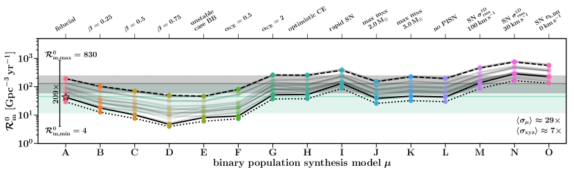
Figure 9: Predicted intrinsic BHNS merger rates for our $420$ model variations. The rates are for mergers at $z=0$ without applying GW selection effects. We show for each of the $15$ binary population synthesis model variations (given in Table 2) the BHNS merger rates for the $28$ variations in SFRD$(Z_{\rm{i}},z)$ (given in Table 3). We connect predictions that use the same SFRD$(Z_{\rm{i}},z)$ model with a line for visualisation reasons only (it is not an interpolation between models). Three SFRD$(Z_{\rm{i}},z)$ variations, xyz$=$000 (solid), xyz$=$231 (dashed) and xyz$=$312 (dotted) are highlighted, corresponding to our fiducial SFRD$(Z_{\rm{i}},z)$ model and the models resulting in one of the highest and lowest rate predictions. The shaded horizontal bars mark the corresponding GW-inferred $90\%$ credible intervals for the merger rate densities from Abbott et al. (2021d): $\mathcal{R}_{\rm{m}}^{0}={45}_{-33}^{+75}$$\,\rm{Gpc}^{-3}$ $\,\rm{yr}^{-1}$ when assuming that GW200105 and GW200115 are representative of the entire BHNS population (teal) and $\mathcal{R}_{\rm{m}}^{0}={130}_{-69}^{+112}$$\,\rm{Gpc}^{-3}$ $\,\rm{yr}^{-1}$ when assuming a broader distribution of component masses (grey). Our fiducial model ($\rm{A}000$) estimate is shown with a star symbol. On the right of the panel $\langle\sigma_{\mu}\rangle$ and $\langle\sigma_{\rm{xyz}}\rangle$ represent the mean scatter in rates due to varying our assumptions in binary population synthesis and SFRD$(Z_{\rm{i}},z)$ prescriptions, respectively. These are calculated using Equation 7 and 8. The minimum and maximum rates and the ratio between those are quoted with an error bar on the left. We use the short-hand notation $\mathcal{R}_{\rm{m}}^{0}\equiv(\mathop{}\!\mathrm{d}{N}_{\rm{det}}^{2}/\mathop{}\!\mathrm{d}{t}_{\rm{s}}\mathop{}\!\mathrm{d}{V}_{\rm{c}})({t}_{\rm{m}}(z=0))$.

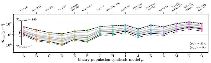
Figure 10: Same as Figure 9 but for the predicted detectable BHNS rates for a GW network at design sensitivity. We use the short-hand notation $\mathcal{R}_{\rm{det}}\equiv\mathop{}\!\mathrm{d}{N}_{\rm{det}}/\mathop{}\!\mathrm{d}{t}_{\rm{det}}$.

4 Varying model assumptions

The predicted rates and characteristics of BHNS mergers, presented in Section 3 for our fiducial model $\rm{A}000$, are sensitive to uncertainties in binary population synthesis and SFRD$(Z_{\rm{i}},z)$ model assumptions. We compare in this section the predicted BHNS merger rates and characteristics for our total of $420$ combinations of the $15$ binary population synthesis and $28$ SFRD$(Z_{\rm{i}},z)$ models. These model variations are summarized in Table 2 and 3. In most figures throughout this section we highlight three of our SFRD$(Z_{\rm{i}},z)$ models: the preferred phenomenological model from Neijssel et al. (2019), $\rm{xyz}=000$, and the SFRD$(Z_{\rm{i}},z)$ prescriptions $\rm{xyz}=312$ and $\rm{xyz}=231$, which we show correspond to the lowest and highest BHNS merger rates, respectively.

4.1 Predicted BHNS merger rate for varying model assumptions

4.1.1 Intrinsic BHNS merger rates

The predicted intrinsic (at redshift $z=0$) rates for BHNS mergers are shown for our $420$ models in Figure 9. These rates are calculated using Equation 2 and do not yet take into account the GW detector selection effects. We find that the intrinsic BHNS merger rates are predicted to lie in the range $\mathcal{R}_{\rm{m}}^{0}\approx$ $4$–$830$ $\,\rm{Gpc}^{-3}$ $\,\rm{yr}^{-1}$. Our fiducial model $\rm{A}000$ predicts $\mathcal{R}_{\rm{m}}^{0}\approx 43$$\,\rm{Gpc}^{-3}$ $\,\rm{yr}^{-1}$. We discuss in more detail the variations in rates over the models in Section 4.1.6. Almost all $420$ models predict intrinsic BHNS merger rates that are consistent with one of the GW inferred $90\%$ confidence interval for the BHNS merger rates from Abbott et al. (2021d).

4.1.2 GW detectable BHNS merger rates

The predicted GW detectable rates for BHNS mergers are shown in Figure 10. These rates are calculated using Equation 2.3 for a ground-based GW detector equivalent to the LVK network at design sensitivity for a full year observing run. Our fiducial model predicts a BHNS merger rate of $\mathcal{R}_{\rm{det}}\approx 11\,\rm{yr}^{-1}.$ Considering the $420$ model variations we find predicted rates in the range $\mathcal{R}_{\rm{det}}\approx 1$–$180\,\rm{yr}^{-1}$. The GW detectable rates in Figure 10 behave similar under our $420$ model variations as the intrinsic rates presented in Figure 9. This is because the impact of the redshift evolution of the BHNS merger properties in our simulations is minor compared to changes over our model variations, within the GW horizon distance of BHNS mergers.

4.1.3 Formation channel rates

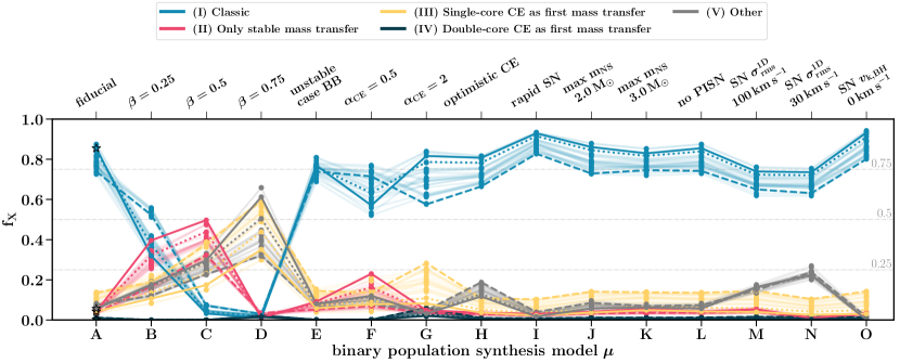
Figure 11: Fraction, $\rm{f}_{\rm{X}}$, that each formation channel contributes to the total predicted GW detected BHNS merger rate $\mathcal{R}_{\rm{det}}$ for our $420$ model variations (where the subscript X is a placeholder for the formation channel label). Labels and lines are as in Figure 10, but are colored based on the five formation channels we classify as described in Section 3.1.

$\rm{f}_{\rm{I}}$	$\rm{f}_{\rm{II}}$	$\rm{f}_{\rm{III}}$	$\rm{f}_{\rm{IV}}$	$\rm{f}_{\rm{V}}$
$0.01$–$0.94$	$0.008$–$0.50$	$0.021$–$0.60$	$0$–$0.59$	$<0.1$–$0.66$

Table 5: Range of the minimum and maximum predicted percentage that each BHNS formation channel contributes when considering all $420$ model variations studied in this work. From left to right the columns represent the formation channels labeled: (I) classic, (II) only stable mass transfer, (III) Single-core CE as first mass transfer, (IV) Double-core CE as first mass transfer and (V) other. The formation channels are described in Section 3.1.

The predicted percentages that each formation channel contributes to the predicted total GW detected BHNS merger rate is affected by variations in SFRD$(Z_{\rm{i}},z)$ and binary population synthesis models and shown in Figure 11 and Table 5 for our five formation channels as described in Section 3.1. The minimum and maximum predicted percentages that each formation channel from Figure 11 can contribute to the GW detected BHNS rate is quoted in Table 5. We find that the fraction each formation channel contributes is dominated by variations in the binary population synthesis model over variations in SFRD$(Z_{\rm{i}},z)$. All models, except those involving binary population synthesis models B, C and D, predict the classic formation channel (I) dominates the BHNS rate, with a percentage $\rm{f}_{\rm{I}}>50\%$ of the GW detectable BHNS coming from this channel. Particularly in models B, C and D, that assume a fixed mass transfer efficiency of $\beta=0.25,\beta=0.5$ and $\beta=0.75$ for non compact objects, respectively, this percentage drastically decreases, as in those models binaries going through the classic channel merge before they form a BHNS system. This is particularly visible in the variations for Figures 4, 5 and 6 for models B and C, which are given in our online supplementary material. All in all, we find that the formation channel contributions for BHNS mergers is particularly sensitive to mass transfer, and so we expect that also varying binary population synthesis prescriptions for the stability criteria, the angular momentum loss and the CE prescription might further impact our results, as also suggested by e.g. Klencki et al. (2020, see Section 4.3).

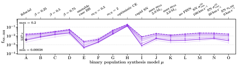
Figure 12: The predicted fractions of detectable BHNS systems where the NS forms first (NS–BH systems), $\rm{f}_{\text{NS--BH}}$, for a GW network at design sensitivity. The labels and lines are as in Figure 9.

4.1.4 GW Detectable NS–BH merger rates

NS–BH systems where the NS forms first are interesting astrophysical sources. First, because the first formed NS may spin up during mass transfer episodes and eventually form a millisecond-pulsar BH binary that might be observable with radio telescopes (e.g. Pfahl et al., 2005; Chattopadhyay et al., 2021). Detecting such a system would provide a unique laboratory to test general relativity and alternative theories of gravity (Wex & Kopeikin, 1999; Kramer et al., 2004; Wex, 2014) and will enable high precision measurements of the properties of BHs (Blandford & Teukolsky, 1975; Brumberg et al., 1975). However, to date, no pulsar–BH system has been observed through radio observations. This might not be entirely surprising as several studies estimate that the fraction of pulsar–BH over NSNS binaries in our Milky Way is small (Pfahl et al., 2005; Chattopadhyay et al., 2021). Currently there are about 20 NSNS known (e.g. Tauris et al., 2017b; Farrow et al., 2019). Second, in NS–BH systems the second formed BH may obtain a high BH spin if its progenitor helium star spun up due to tidal interactions with the NS companion, whereas a first formed BH in BHNS mergers may always have negligible spin (Qin et al., 2018). NS–BH mergers might, therefore, be distinguishable in GW observations by measuring a high $\chi_{\rm{eff}}$ from the high NS or BH spins compared to BH–NS mergers that will always have low $\chi_{\rm{eff}}$ (e.g. Chattopadhyay et al., 2021).

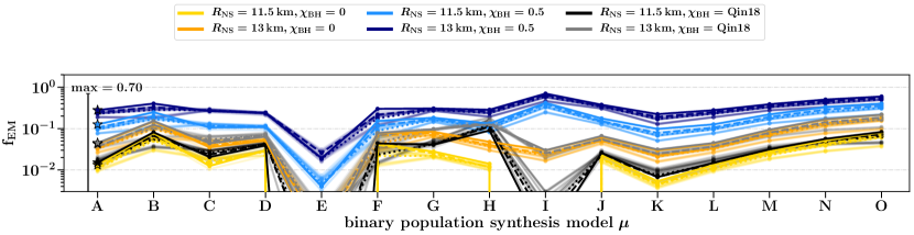
Figure 13: The fraction of GW detected BHNS mergers in which the NS is disrupted outside of the BH innermost stable circular orbit (instead of plunging into the BH), $\rm{f}_{\rm{EM}}$. Different colors correspond to different assumptions for the NS radii and BH spins. The labels and lines are as in Figure 9.

Figure 12 shows the predicted fraction of detectable BHNS mergers where the NS formed first (NS–BH systems). We predict fractions of NS–BH mergers in the range $\rm{f}_{\text{NS--BH}}\approx 0.00038$–$0.2$ for a GW network equivalent to LVK at design sensitivity. The highest fraction of NS–BH mergers is in the optimistic-CE model (H). This is because most NS–BH systems form from binaries where the first mass transfer occurs relatively early on (case A or early case B mass transfer). In our model this phase of mass transfer is typically highly conservative and the stars can therefore exchange a large fraction of mass and reverse in masses, making the initial primary star the least massive star in the system and eventually form the NS first. Such systems also typically undergo a CE phase initiated by a donor star on the Hertzsprung gap, which are assumed to lead to a stellar merger in the pessimistic CE models. From Figure 12 it can be seen that the fraction of GW detectable NS–BH mergers is particularly sensitive to assumptions in the mass transfer and CE prescriptions, varied in binary population synthesis models B, C, D, E, F, G and H. GW observations of $\chi_{\rm{eff}}$ of BHNS mergers could therefore be particularly insightful to constraining the mass transfer and CE prescriptions, given that the spin properties of NS–BH are distinct from those of BH–NS mergers.

4.1.5 GW detectable merger rates of BHNS systems that disrupt the NS outside of the BH innermost-stable orbit

Figure 13 shows the predictions for the fraction of GW detectable BHNS mergers for which the NS is disrupted outside the BH innermost stable circular orbit for six combinations of assumed NS radii and BH spins (described in Section 2.6). Our $420$ model variations predict fractions in the range $\rm{f}_{\rm{EM}}\approx 0$–$0.70$. The predictions that assume the highest BH spin values predict the highest fraction of BHNS mergers that disrupt the NS outside of the BH innermost stable orbit. Larger NS radii assumptions also lead to higher fractions as this makes it easier to disrupt the NS. The unstable case BB model (E) and rapid SN remnant mass prescription model (I) give the lowest fractions, where for the 11.5$\,\rm{km}$ NS radius and zero or Qin et al. (2018) BH spin assumptions none of the BHNS systems disrupt the NS outside of the BH. This is because only BHNS mergers with small NS and BH masses disrupt the NS outside of the BH innermost stable circular orbit for these most pessimistic assumptions for the NS radii and BH spins (see dark gray shaded area in top panels of Figure 6). These low mass remnants form from relatively low mass helium stars, that in model E undergo unstable case BB mass transfer and merge before forming a BHNS system. Model I does not produce, by construction, any BHs with $m_{\rm{BH}}\lesssim 6$$\,\rm{M}_{\odot}$, which are the BH masses that can disrupt the NS outside of the BH for the most pessimistic NS radius and BH spin assumption. At the same time, model I also predicts the highest fraction of NS disruptions outside the BH innermost-stable orbit, as high as $\rm{f}_{\rm{EM}}\approx 0.70$ for the most optimistic assumptions of 13$\,\rm{km}$ NS radii and BH spins of ${\chi}_{\rm{BH}}=0.5$. This is because the rapid SN remnant prescription produces a peak of BHs with masses around $\sim 8\,\rm{M}_{\odot}$ that disrupt their NS under these assumptions.

Figure 13 shows that the predicted rates of BHNS mergers that disrupt the NS outside of the BH innermost-stable orbit that assume our Qin et al. (2018) spin model (black and gray lines) are closest to our models that assume all BHs have zero spins (yellow and orange lines). This is because in most BHNS mergers the BHs forms first, resulting in zero BH spins in our Qin et al. (2018) spin model. The only binary population synthesis model where the Qin et al. (2018) spin assumption predicted rates drastically deviate from the zero BH spin predicted rates is in the optimistic-CE model (H). This is because in this model the fraction of NS–BH mergers, where the NS formed first, can be as high as $\rm{f}_{\text{NS--BH}}\approx 20\%$ as shown in Figure 12. As a result, a significant fraction of these NS–BH can achieve high spins in our Qin et al. (2018) model and disrupt the NS outside of the BH innermost-stable orbit.

The disruption of the NS outside of the BH innermost stable circular orbit can result in the production of electromagnetic transients such as short gamma-ray bursts, neutrinos and kilonovae (e.g. Bhattacharya et al., 2019; Barbieri et al., 2020; Darbha et al., 2021). In a (small) fraction of such events the electromagnetic counterpart might be detectable, allowing a multi-messenger observation (e.g. a fraction 0.1–0.5 for kilonoavae cf. Bhattacharya et al., 2019; Zhu et al., 2020). This depends among other things on the distance to the BHNS merger, the luminosity of the electromagnetic transient, its orientation and sky location.

4.1.6 Effect of varying binary population synthesis and SFRD$(Z_{\rm{i}},z)$ assumptions on the predicted BHNS rates

To quantify the scatter in the predicted rates, i.e. the impact from varying our model assumptions, we calculate the mean of the ratios between the maximum and minimum predicted rates given by

$$\langle\sigma_{\rm{\mu}}\rangle=\frac{1}{15}\sum_{\mu=A}^{\mu=O}\frac{\rm{max}(\mathcal{R}_{\rm{m,\mu 000}}^{0},...,\mathcal{R}_{\rm{m,\mu 333}}^{0})}{\rm{min}(\mathcal{R}_{\rm{m,\mu 000}}^{0},...,\mathcal{R}_{\rm{m,\mu 333}}^{0})},$$ (7)

and

$$\langle\sigma_{\rm{xyz}}\rangle=\frac{1}{28}\sum_{\rm{xyz}=000}^{\rm{xyz}=333}\frac{\rm{max}(\mathcal{R}_{\rm{m,Axyz}}^{0},...,\mathcal{R}_{\rm{m,Oxyz}}^{0})}{\rm{min}(\mathcal{R}_{\rm{m,Axyz}}^{0},...,\mathcal{R}_{\rm{m,Oxyz}}^{0})}.$$ (8)

The values for the scatter caused by our binary population synthesis and SFRD$(Z_{\rm{i}},z)$ assumptions are quoted for our BHNS mergers in Figure 9 and 10. We find that for both the predicted intrinsic and detected BHNS merger rates $\langle\sigma_{\rm{\mu}}\rangle\approx 20$–$30$ and $\langle\sigma_{\rm{xyz}}\rangle\approx 8$. Overall, we thus find that variations from binary population synthesis and SFRD$(Z_{\rm{i}},z)$ assumptions affect the rates of order $\sim\mathcal{O}(10)$. In the models that we varied we find that the binary population synthesis variations impact the rate with a factor 2–4 more compared to the variations in SFRD$(Z_{\rm{i}},z)$. Figure 9 and 10 also show that the uncertainties are somewhat independent of each other: our SFRD$(Z_{\rm{i}},z)$ assumptions introduce uncertainties of $\mathcal{O}(10)$ for all our binary population synthesis models, and vice versa: varying our binary population synthesis model assumptions introduces uncertainties of order $\mathcal{O}(10)$ for all our SFRD$(Z_{\rm{i}},z)$ models. This is because in all our population synthesis models, the BHNS rate behaves overall similarly as a function of metallicity: the rate is suppressed both at extremely low and high metallicities for all our binary population synthesis variations. This is shown for our fiducial model in Figure 5.

4.1.7 Effect from binary population synthesis variations

The highest predicted BHNS rates in Figure 9 and 10 are found in the binary population synthesis models G, H, I, K, M, N and O, which have $\gtrsim 50\%$ of the SFRD$(Z_{\rm{i}},z)$ variations typically predict BHNS merger rates $\mathcal{R}^{0}\gtrsim 100$$\,\rm{Gpc}^{-3}$ $\,\rm{yr}^{-1}$ and predict for most SFRD$(Z_{\rm{i}},z)$ models $\mathcal{R}_{\rm{det}}\gtrsim 10$$\,\rm{yr}^{-1}$.

In model G the CE efficiency parameter is increased to $\alpha=2$ compared to $\alpha=1$ for our fiducial model. This means that we assume more binary orbital energy is converted into unbinding the CE during the unstable mass transfer phase. This leads to more binaries surviving the CE phase as systems that don’t successfully eject the envelope are assumed to merge as stars. The result is that the rate of BHNS mergers forming from formation channels involving a CE, increases in our simulations for model G, as also visible for model G in Figure 11. The optimistic CE model (H) is the variation on our fiducial model where we allow Hertzsprung gap donors that engage in a CE event to survive. In this model the BHNS merger rate is, therefore, enhanced compared to the fiducial model as a significant number of BHNS systems forms through a CE with a Hertzsprung gap donor. Figure 12 shows that model H is especially important for forming a large fraction of NS–BH systems. In the rapid SN model (I) the rate of BHNS merger formation is also enhanced compared to our fiducial model that assumes the delayed SN remnant mass prescription. This is because most BHNS mergers form from binaries with secondary stars that have $10\lesssim m_{2,\rm{i}}/\,\rm{M}_{\odot}\lesssim 30$ (Section 3.2 and top panels Figure 4). The rapid SN remnant mass function typically allows a larger fraction of secondary masses in this range to form a NS whereas in the delayed prescription these form a BH instead. This is visible in the bottom panel in Figure 12 of Fryer et al. (2012). This effect causes the BHNS rate to increase in our model I simulation. In model K, which assumes a maximum NS mass of $3$$\,\rm{M}_{\odot}$, the BHNS merger rate is also enhanced as a fraction of the systems that in our fiducial model form BHBH mergers with one BH $\lesssim 3\,\rm{M}_{\odot}$ in this model form a BHNS merger instead. Models M, N and O all have lower BH and/or NS natal kicks compared to our fiducial model, which increases the fraction of systems that remain bound during the SNe and therefore increases the BHNS merger rate compared to our fiducial model.

In Figure 9 and 10 show that when the mass transfer efficiency is changed to respectively $\beta=0.25,0.5$ and $0.75$ (models B, C and D) that this leads to a decreasing BHNS rate. This seems counter-intuitive since higher values for $\beta$ correspond to more mass accretion by a star during mass transfer, which intuitively leads to the formation of more BHs and higher BHNS merger rates. However, there is another effect: the detectable systems are highly biased towards tight binaries that merge within a Hubble time. As almost all our BHNS mergers in our fiducial model go through the classic formation channel (I) (Figure 11) which involves a CE phase, a more massive companion leads to a more massive shared envelope that needs to be successfully ejected to avoid a stellar merger from the CE event. This leads to fewer BHNS systems as in agreement with findings by e.g. Kruckow et al. (2018). Figure 12 shows that the fraction of NS–BH mergers, on the other hand, increases for increasing $\beta$. This is because in this case the contribution of systems that merge as a result from a failed CE ejection is relatively low as these binaries typically form from initially lower mass stars and will typically have a lower mass envelope in the CE compared to BH–NS binaries.

4.1.8 Effect from SFRD$(Z_{\rm{i}},z)$ variations

For a given binary population synthesis model, the highest predicted BHNS rates are from the SFRD$(Z_{\rm{i}},z)$ models with the Langer & Norman (2006) MZR (the models $\rm{xy}1$). For a fixed galaxy mass, this MZR relation results in lower average birth metallicities compared to the other MZR variations as can be seen in Figure LABEL:fig:MSSFR-MZRs (see Appendix A of Neijssel et al. 2019 for more details). This leads to a higher fraction of stars that form BHs and therefore to a higher yield of BHNS mergers. The other two MZRs, Langer & Norman (2006) $+$ offset and Ma et al. (2016), corresponding to $\rm{xy}2$ and $\rm{xy}3$ respectively, lead to lower BHNS yields. We find that the MZR dominates the uncertainty in the predicted rates for our model variations, consistent with findings by e.g. Artale et al. (2019); Chruslinska & Nelemans (2019).

For the SFRD we find that the Strolger et al. (2004) SFRD ($2\rm{yz}$) typically has the highest yields, followed by the Madau & Dickinson (2014) ($1\rm{yz}$) and Madau & Fragos (2017) ($3\rm{yz}$) SFRD assumptions. This is corresponds to each SFRD$(Z_{\rm{i}},z)$ prescription having a different total star forming yield, as can be seen in Figure LABEL:fig:MSSFR-SFRs.

For the GSMFs we find the highest yield is given by the Furlong et al. (2015) functions, either single or double Schechter, which both give almost identical yields. On the other hand, the Panter et al. (2004) GSMF ($\rm{x}1\rm{z}$) leads to relatively lower BHNS merger yields. This is because the Furlong et al. (2015) GSMF prescriptions have relatively more low mass galaxies compared to the Panter et al. (2004) GSMF as can be seen in Figure LABEL:fig:MSSFR-GSMFs, which map to lower $Z_{\rm{i}}$ and typically to higher BHNS yields.

In total this leads to the SFRD$(Z_{\rm{i}},z)$ models $\rm{xyz}=231$ and $\rm{xyz}=312$ having (one of) the highest and lowest BHNS merger yields for each binary population synthesis model, as can be seen in Figures 9 and 10. Our fiducial SFRD$(Z_{\rm{i}},z)$ model (000) also produces one of the lowest yields. These three SFRD$(Z_{\rm{i}},z)$ models are highlighted in Figures 9–13.

Figure 14: Predicted normalized probability distribution functions (PDFs) for BHNS merger characteristics for our $420$ model variations of binary population synthesis and SFRD$(Z_{\rm{i}},z)$ assumptions (Tables 2 and 3). Each row shows, for the $15$ binary population synthesis variations (denoted with letters A, B, …, O, and different colors), the PDFs for the $28$ SFRD$(Z_{\rm{i}},z)$ models in a subfigure using a kernel density estimator. The PDF axis is plotted in linear scale. All distributions are weighted by the detection probability for an observatory equivalent to the LVK network at design sensitivity. For the kernel density functions we use the dimensionless bandwidth. More details are given in https://github.com/FloorBroekgaarden/BlackHole-NeutronStar.

4.2 Predicted BHNS distribution functions for varying model assumptions

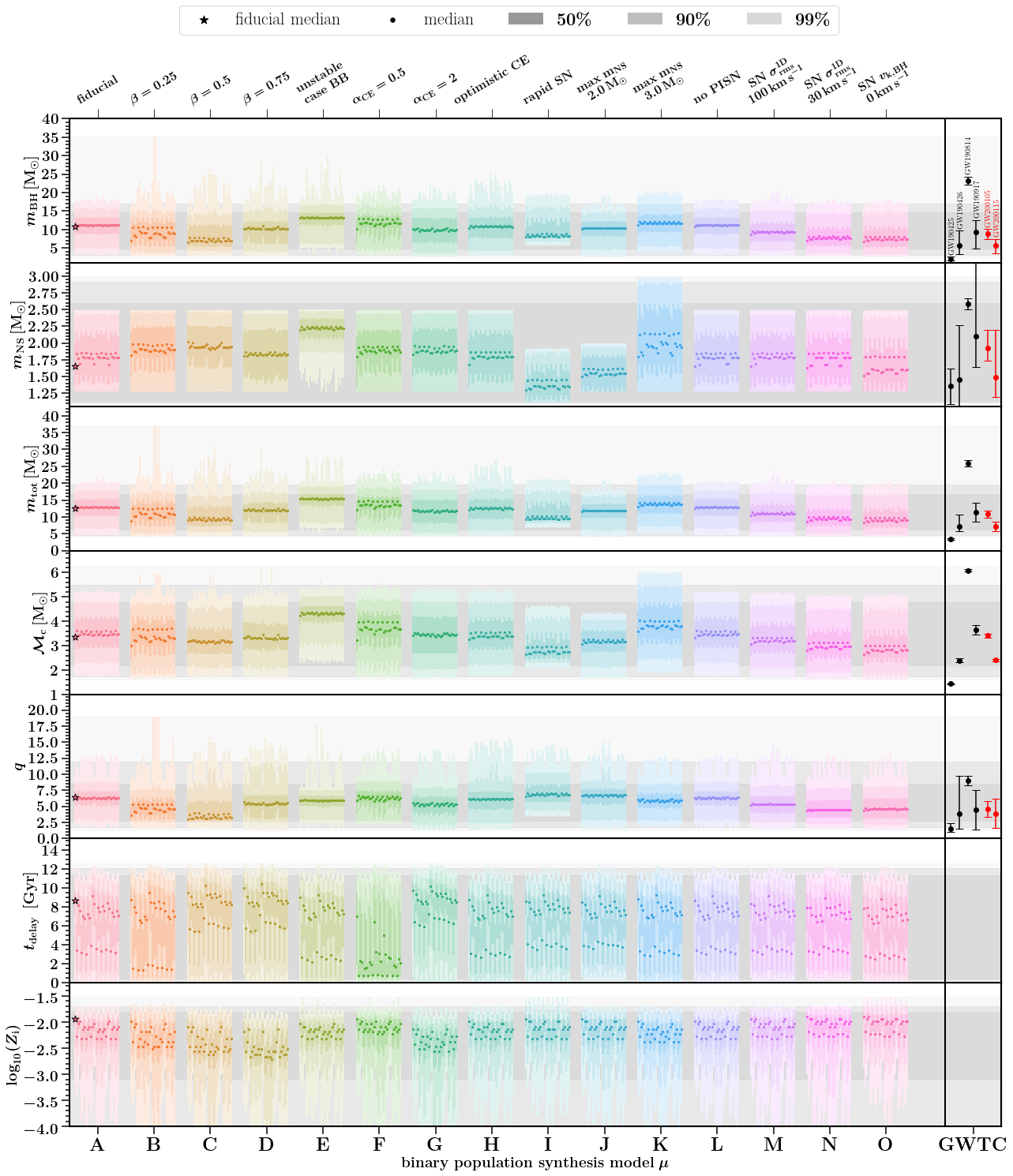
Figure 15: Distribution quantiles for the predicted BHNS distributions for our $420$ model variations of binary population synthesis and SFRD$(Z_{\rm{i}},z)$ assumptions (Table 2 and 3). Panels, colors and labels are as in Figure 14. Each colored block, which corresponds to one sub-figure in Figure 14, shows 28 bars, indicating the 28 SFRD$(Z_{\rm{i}},z)$ model variations. The SFRD$(Z_{\rm{i}},z)$ labels of these bars are shown in Figure 17. Each individual vertical bar representing one SFRD$(Z_{\rm{i}},z)$ model shows the median (scatter points), $50\%$ , $90\%$ and $99\%$ (see three shades) quantiles for the normalized probability distribution functions. The fiducial model ($\rm{A}000$) median values are shown with star symbols. The gray areas in the background show the minimum and maximum values for the $50\%$, 90$\%$ and 99$\%$ distribution quantiles for all $420$ models in each panel. All distributions are weighted by the detection probability for an observatory equivalent to the LVK network at design sensitivity. The rightmost columns show the median and $90\%$ credible intervals for the component masses, total mass, chirp mass and mass ratio of the confident BHNS detections GW200105 and GW200115 in red (Abbott et al., 2021d) and the possible detected GW sources GW190425, GW190426, GW190814 and GW190917 in black (where a BHNS origin has not been ruled out yet; Abbott et al. 2021b, a).

Besides the predicted rates (discussed in Section 4.1), the shapes of the predicted BHNS distributions are also sensitive to the binary population synthesis and SFRD$(Z_{\rm{i}},z)$ assumptions. To summarize and compare these effects, we discuss in this section the shape of the BHNS merger distributions for our $420$ model variations. We show the BH and NS masses ($m_{\rm{BH}}$ and $m_{\rm{NS}}$), mass ratio ($q_{\rm{f}}=m_{\rm{BH}}/m_{\rm{NS}}$), total mass ($m_{\rm{tot}}=m_{\rm{BH}}+m_{\rm{NS}}$) and chirp mass (${\mathcal{M}}_{\rm{c}}$) distributions as these are properties of the BHNS mergers that are generally inferred from GW observations. In addition, we show the delay times, ${t}_{\rm{delay}}$ and birth metallicity, $Z_{\rm{i}}$, of the detected mergers. The birth metallicity is highly correlated with the inspiral times, shown in previous sections, as BHNS mergers with longer inspiral times typically formed from stars with lower $Z_{\rm{i}}$. Throughout this section we show normalized probability distribution functions of these BHNS characteristics, to compare their shapes (the rates are given in Figure 9 and  10). The distributions are weighted for the detection probability obtained from Equation 2.3 for a GW detector equivalent to the LVK network at design sensitivity.

To summarize and compare the shape of the BHNS merger characteristics for $420$ model variations we focus on two figures. First, Figure 14 shows the predicted BHNS probability distribution functions for all $420$ model variations. This figure visualizes the overall shape of the distributions. Second, Figure 15, shows the median and the $50\%$, $90\%$ and $99\%$ distribution quantiles for all $420$ model variations.

4.2.1 BH mass

The top panel in Figure 15 shows that for all our $420$ model variations $90\%$ of the predicted observable BHNS mergers have $m_{\rm{BH}}$ in the range $2.5$–$18\,\rm{M}_{\odot}$. We find that in all model combinations less than $5\%$ of the BHNS mergers are predicted to have $m_{\rm{BH}}$ exceeding $18$$\,\rm{M}_{\odot}$. Moreover, most of the $420$ model variations predict $<1\%$ of GW detectable BHNS mergers have $m_{\rm{BH}}\gtrsim 20\,\rm{M}_{\odot}$, and only in models B, C, D and H this fraction is slightly above $1\%$ for some of the SFRD$(Z_{\rm{i}},z)$ models. This is especially clear in the probability distribution functions (PDFs) for the BH mass shown in Figure 14, where the region above $m_{\rm{BH}}\gtrsim 20\,\rm{M}_{\odot}$ is visibly suppressed for all models. Even the models that do not assume (pulsational)-PISN (all models with $\mu=\rm{L}$), or that have SFRD$(Z_{\rm{i}},z)$ models that prefer low $Z_{\rm{i}}$, lack a population of BHNS mergers with $m_{\rm{BH}}\gtrsim 20\,\rm{M}_{\odot}$. All in all, we conclude that such massive BHs are extremely rare in BHNS mergers in all our $420$ model variations. Detecting more than 1$\%$ of BHNS mergers with $m_{\rm{BH}}\gtrsim 20$$\,\rm{M}_{\odot}$ would therefore suggest that a large fraction of the BHNS systems form through a different formation channel than the isolated binary evolution channel, such as in AGN disks or through dynamical formation, which predict a significant fraction of BHNS mergers with BHs exceeding 20$\,\rm{M}_{\odot}$ (e.g. Rastello et al., 2020). Alternatively, it could constrain binary population synthesis and SFRD$(Z_{\rm{i}},z)$ models as basically all our models would be excluded as they do not support such observations. In Broekgaarden et al. (in prep.) we show that this is very different compared to our results for BHBH mergers, where typically our models predict that $\gtrsim 50\%$ of GW detectable BHBH mergers contain two BHs that both have masses $m_{\rm{BH}}$ exceeding $18\,\rm{M}_{\odot}$.

The $m_{\rm{BH}}$ distributions for models with the rapid SN remnant mass model (I) sharply peak around $m_{\rm{BH}}\approx 8\,\rm{M}_{\odot}$ in Figure 14. This is because the rapid prescription maps a large range of ZAMS masses to this BH mass range (see Figure 12 of Fryer et al., 2012)

The top panel in Figure 14 and 15 also show that BHNS mergers with $m_{\rm{BH}}\lesssim$5$\,\rm{M}_{\odot}$ are rare in most of our $420$ models. In all models, except most of the SFRD$(Z_{\rm{i}},z)$ models in combination with E (unstable case BB mass transfer) and all models with I (rapid SN remnant mass model) about $5\%$ of BHNS are expected to have BH masses below $5\,\rm{M}_{\odot}$. The sharp boundary in the minimum BH mass for model I is caused by the rapid SN remnant mass prescription, which assumes no BHs form with $m_{\rm{BH}}\leq 6\,\rm{M}_{\odot}$. Figure 14 and  15 show that models including B, C, G, H, N and O have the largest fraction of BHNS mergers with $m_{\rm{BH}}\lesssim 5$$\,\rm{M}_{\odot}$.

4.2.2 NS mass

The $90\%$ confidence intervals of the BHNS NS masses in the second row of Figure 15 typically span the range $m_{\rm{NS}}\approx 1.25$–$2.5$$\,\rm{M}_{\odot}$. The exceptions of models where the $90\%$ quantiles shift significantly are model E (assuming unstable case BB) where the range is $m_{\rm{NS}}\approx 1.8$–$2.5$$\,\rm{M}_{\odot}$, model I (the rapid SN remnant mass model) where it shifts to $m_{\rm{NS}}\sim 1.1$–$1.9$, model J (assuming max $m_{\rm{NS}}=2\,\rm{M}_{\odot}$) where it shifts to $1.25$–$2$$\,\rm{M}_{\odot}$ and model K (assuming max $m_{\rm{NS}}=3\,\rm{M}_{\odot}$) where it shifts to $1.25$–$3$$\,\rm{M}_{\odot}$. Especially in Figure 14 it can be seen that the unstable case BB model highly favors NSs with $m_{\rm{NS}}\gtrsim 2\,\rm{M}_{\odot}$, which is a result from that the low mass NSs are suppressed as their low mass progenitor helium stars typically undergo a case BB mass transfer phase and merge before forming a BHNS system in this model. In addition, it can be seen that for the rapid SN remnant mass model (I) the most probable NS mass in BHNS mergers is predicted to be $\lesssim 1.25$$\,\rm{M}_{\odot}$. In most model variations we find that the median NS mass is $\gtrsim 1.8\,\rm{M}_{\odot}$ and that except for models I and J, in all other models typically $\gtrsim 25\%$ of GW detectable BHNS mergers have NS with $m_{\rm{NS}}\gtrsim 2\,\rm{M}_{\odot}$. Such massive NSs are thus predicted to be common in BHNS mergers as can also be seen in the Figure 14 and 15.

4.2.3 Total mass and chirp mass

The BHNS total mass distributions follow the shape of the BH mass distributions as the BH typically dominates the mass of the BHNS. Figure 15 shows that in all $420$ model variations $90\%$ of the predicted GW detectable BHNS mergers will have $m_{\rm{tot}}$ in the range $\sim 5$–$20\,\rm{M}_{\odot}$ and hence that less than $5\%$ of BHNS mergers are predicted to have $m_{\rm{tot}}\gtrsim 20\,\rm{M}_{\odot}$. The total mass peaks around $m_{\rm{tot}}\approx 15\,\rm{M}_{\odot}$ for models including our fiducial model (A), and has the highest average in the unstable case BB model (E), as shown in Figure 14, as in this model many of the binaries with low BH mass progenitors merge during unstable case BB mass transfer. The total mass peaks as low as $m_{\rm{tot}}\approx 7\,\rm{M}_{\odot}$ for models including model C ($\beta=0.5$) and models N and O with low SN natal kicks. The latter is because low mass BHs can get moderate kicks in our delayed remnant mass prescription, disrupting the binary, whereas in models N and O such low mass BHs are given low or zero natal kicks.

Figure 15 shows that $90\%$ of the predicted GW detectable BHNS mergers will have ${\mathcal{M}}_{\rm{c}}\approx 1.7$–$5.5\,\rm{M}_{\odot}$ and hence that less than $5\%$ of BHNS mergers are predicted to have ${\mathcal{M}}_{\rm{c}}\gtrsim 5.5\,\rm{M}_{\odot}$. The most probable chirp masses, as shown in Figure 14, are typically in the range ${\mathcal{M}}_{\rm{c}}\approx 2$–$5$$\,\rm{M}_{\odot}$.

4.2.4 Mass ratio distribution

The $90\%$ quantiles for the BHNS mass ratio distributions lies for all models in $q_{\rm{f}}\approx 2$–$12$ as shown in Figure 15. The median and most probable BHNS $q_{\rm{f}}$ for our fiducial model (A), and most models, is $q_{\rm{f}}\approx 6$ as shown in Figure 14. For models B, C and D ($\beta=0.25,0.5,0.75)$, however, this changes to a sharper peak around $q_{\rm{f}}\approx 3$, as in these models low mass BHs are more common. Figure 15 also shows that in none of the models more than 5$\%$ of the BHNS mergers are predicted to have $q_{\rm{f}}$ $\gtrsim 12$. In addition, Figure 14 and  15 show that BHNS mergers with $q_{\rm{f}}\lesssim 2$ are predicted to be rare in all our $420$ model variations (less than $5\%$ of all BHNS mergers).

4.2.5 Delay times

Figures 14 and  15 show that the predicted delay time distributions have a wide spread of ${t}_{\rm{delay}}$, which typically peaks around 9$\,\mathrm{Gyr}$ or 1$\,\mathrm{Gyr}$, where the peak depends mostly on the SFRD$(Z_{\rm{i}},z)$ model that is used. Figure 15 shows that SFRD$(Z_{\rm{i}},z)$ models with relatively shorter median delay times (e.g. models with xy1), correspond to SFRD$(Z_{\rm{i}},z)$ models with low median metallicities. This is because the delay time of the detected BHNS mergers is a convolution between the intrinsic delay time distribution and the SFRD$(Z_{\rm{i}},z)$. Intrinsically, most BHNS mergers have short delay times $\lesssim 1\,\mathrm{Gyr}$ (e.g. Figure 7), and so the majority of BHNS systems has already merged before redshift $z=0$. In addition, the yield of BHNS mergers is higher at lower metallicities (i.e., around $\log_{10}(Z_{\rm{i}})\approx-2.5$), as shown in Figure 5. As a result, SFRD$(Z_{\rm{i}},z)$ models with high median metallicities only form stars with low $Z_{\rm{i}}$ early in the Universe. Because of the high BHNS formation yield, these low metallicities dominate the rate, leading to the detected population having longer delay times (since the BHNS with short delay times from low metallicities will already have merged at high redshifts). On the other hand, SFRD$(Z_{\rm{i}},z)$ models with low median metallicities still form low $Z_{\rm{i}}$ binaries at lower redshifts. All in all, this results in SFRD$(Z_{\rm{i}},z)$ models with low median metallicities corresponding to shorter ${t}_{\rm{delay}}$ values.

4.2.6 Birth metallicities

Figures 14 and  15 show that the predicted range and shape of the birth metallicity distribution of the detected BHNS mergers is strongly impacted by the SFRD$(Z_{\rm{i}},z)$ prescriptions. The scatter is mostly dominated by the MZR prescriptions in combination with the inspiral time distributions from the BHNS mergers. Models with relatively higher metallicities originate from SFRD$(Z_{\rm{i}},z)$ prescriptions that have the Langer & Norman (2006) $+$ offset or Ma et al. (2016) MZR relation that, for a given galaxy mass, map to higher average initial metallicities. Figure 14 shows that typically the metallicities have values in the range $Z_{\rm{i}}\approx 0.001$–$0.03$. The highest values for the median of $Z_{\rm{i}}$ in Figure 15 are $Z_{\rm{i}}$ $\sim 0.016$, whereas the lowest median values are $Z_{\rm{i}}$ $\sim 0.0018$.

4.2.7 Effect from variations in the binary population synthesis and SFRD$(Z_{\rm{i}},z)$ model assumptions on the shape of the BHNS distribution functions

We find that the variation in the predicted BHNS distribution functions is typically dominated by the binary population synthesis model assumptions when comparing with the effect from variations in our SFRD$(Z_{\rm{i}},z)$ models. This can be seen in Figures 14 and 15, that show that typically variations between models that use the same binary population synthesis model but different SFRD$(Z_{\rm{i}},z)$ are smaller compared to variations in the predicted BHNS merger distributions between different binary population synthesis models. The main exception are the $Z_{\rm{i}}$ distributions, which are mostly impacted by variations in SFRD$(Z_{\rm{i}},z)$. Models where some of the probability density function values change with factors 2 or more over variations of SFRD$(Z_{\rm{i}},z)$ within the same binary population synthesis model include $\mu=\rm{B}$ ($\beta=0.25$), $\mu=\rm{F}$ ($\alpha_{\rm{CE}}=0.5$), $\mu=\rm{N}$ (reduced SN natal kicks of $\sigma_{\rm{rms}}^{\rm{1D}}=30\,\rm{km}\,\rm{s}^{-1}$) and $\mu=\rm{O}$ (zero BH natal kicks). This is particularly also visible in Figure 15, where for those binary population synthesis models the median changes the most over SFRD$(Z_{\rm{i}},z)$ variations. In all the figures the largest impact by SFRD$(Z_{\rm{i}},z)$ models comes from the MZR assumption, which seems to be an outlier in our SFRD$(Z_{\rm{i}},z)$ models.

4.2.8 Comparison with GW observations

The right-most panels of Figure 15 show the median and $90\%$ credible intervals for the component masses, total mass, chirp mass and mass ratio of the two confident and four possible BHNS mergers from the third LIGO-Virgo-KAGRA observing run (Abbott et al., 2021d, b, a).

GW200105 and GW200115 are the first two confident BHNS mergers recently detected by LIGO-Virgo (Abbott et al., 2021d). The $90\%$ credible intervals of the properties of GW200105 are inferred to be ${\mathcal{M}}_{\rm{c}}=3.41^{+0.08}_{-0.07}$, $m_{\rm{tot}}=10.9_{-1.2}^{+1.1}$$\,\rm{M}_{\odot}$, $m_{\rm{BH}}=8.{9}_{-1.5}^{+1.2}$ $\,\rm{M}_{\odot}$, $m_{\rm{NS}}=1.{9}_{-0.2}^{+0.3}$ $\,\rm{M}_{\odot}$ and $q_{\rm{f}}=0.22_{-0.04}^{+0.08}$. For GW200115 the properties are ${\mathcal{M}}_{\rm{c}}=2.42_{-0.07}^{+0.05}$$\,\rm{M}_{\odot}$, $m_{\rm{tot}}=7.1_{-1.4}^{+1.5}$$\,\rm{M}_{\odot}$, $m_{\rm{BH}}=5.{7}_{-2.1}^{+1.8}$ $\,\rm{M}_{\odot}$ and $m_{\rm{NS}}=1.{5}_{-0.3}^{+0.7}$$\,\rm{M}_{\odot}$ and $q_{\rm{f}}\equiv(m_{\rm{NS}}/m_{\rm{BH}})=0.26_{-0.10}^{+0.35}$. Both GW200105 and GW200115 are consistent with the predicted distributions from our population synthesis models as shown in Figure 15. However, BHNS mergers with lower black hole masses, such as in GW200115, are more common in a subset of our models such as the simulations with $\beta=0.25$ or $\beta=0.5$ (models B and C) and/or low SN natal kicks (models N and O). In Broekgaarden & Berger (2021) we discuss the formation of GW200105 and GW200115 from isolated binary evolution in more detail and show that our models with low SN kick can potentially explain their formation as well as simultaneously match the inferred BHNS, BHBH and NSNS merger rate densities.

GW190425 is the system of the possible BHNS detections with the lowest total mass and is most likely a NSNS merger. However, a BHNS has not been ruled out. If it is a BHNS system, the component masses are $m_{\rm{BH}}=2.0_{-0.3}^{+0.6}$ and $m_{\rm{NS}}={1.4}_{-0.3}^{+0.3}$, and ${\mathcal{M}}_{\rm{c}}$, $m_{\rm{tot}}$ and $q_{\rm{f}}$ are as shown with errorbars in Figure 15. The inferred credible intervals of GW190425, particularly those for the $m_{\rm{BH}}$, $m_{\rm{tot}}$ and ${\mathcal{M}}_{\rm{c}}$, fall outside of the typical parameter values predicted by our models, which might indicate this is likely not a (typical) BHNS system.

GW190426 (short for GW190426$\_$152155) is a candidate event with a relatively high FAR of 1.4 $\,\rm{yr}^{-1}$ (Abbott et al., 2021b), making it a less significant detection compared to the two events mentioned above. If this event is real, we find that its inferred parameter credible intervals match well with the predicted BHNS distributions for all shown parameters in Figure 15.

GW190814 has been interpreted as a likely BHBH merger since its lower component mass is $2.59_{-0.009}^{+0.008}$$\,\rm{M}_{\odot}$. However, a BHNS interpretation cannot be ruled out (Abbott et al., 2020e). We find that although our model K (max $m_{\rm{NS}}=3.0\,\rm{M}_{\odot}$) can produce such a massive NS, the other inferred credible intervals for GW190814, such as $m_{\rm{tot}}$, ${\mathcal{M}}_{\rm{c}}$ and $m_{\rm{BH}}$, do not match well with typical BHNS distributions predicted by any of our models. These findings are conform Zevin et al. (2020b) who also discuss the challenges in forming this system through isolated binary evolution.

GW190917 is a marginal BHNS event from the GWTC-2.1 catalog (Abbott et al., 2021a). If real, this BHNS merger has inferred source parameters of ${\mathcal{M}}_{\rm{c}}=3.7^{+0.2}_{-0.2}$$\,\rm{M}_{\odot}$, $m_{\rm{BH}}=9.3^{+3.4}_{-4.4}$$\,\rm{M}_{\odot}$, $m_{\rm{NS}}=2.1^{+1.5}_{-0.5}$$\,\rm{M}_{\odot}$ and $q_{\rm{f}}=0.23^{+0.52}_{-0.09}$, very similar to GW200105, that are consistent with our predicted populations.

5 Discussion

5.1 Uncertainties beyond our models

We have modeled the rate and properties of BHNS mergers and demonstrated that uncertainties from both the massive (binary) star evolution and SFRD$(Z_{\rm{i}},z)$ significantly impact the predicted results. However, even with our large set of $420$ model variations, there are still additional uncertainties in the modelling that should be added and further explored in future work. We discuss the most important ones below.

5.1.1 SN remnant mass functions

Figure 14 showed that model I, which uses the rapid SN remnant mass prescription from Fryer et al. (2012), is the model variation that resulted in one of the most drastic changes in the predicted BHNS distributions. This makes the remnant mass prescription one of the key assumptions in modelling BHNS merger properties. Many binary population synthesis studies use the rapid SN prescription instead of our default delayed SN remnant prescription (e.g. Klencki & Nelemans, 2019; Belczynski et al., 2020). The rapid prescription assumes SN explosions occur within 250 ms (compared to longer timescales assumed for the delayed prescription) and reproduces, by construction, the lower remnant mass gap between NSs and BHs that has been inferred from X-ray binary observations (Bailyn et al., 1998; Özel et al., 2010; Farr et al., 2011) by a lack of BHs in the mass range between about the heaviest neutron stars $\sim$ 3$\,\rm{M}_{\odot}$ (Özel & Freire, 2016; Margalit & Metzger, 2017; Cromartie et al., 2020; Abbott et al., 2020b; Sarin et al., 2020) and BHs of $\sim$ 6$\,\rm{M}_{\odot}$.

It is still under debate whether this lower BH mass gap exists. Models of SNe predict a gap (Kochanek, 2014; Pejcha & Thompson, 2015) and no gap (e.g. Woosley & Weaver 1995; Fryer & Kalogera 2001; Ertl et al. 2020; Chan et al. 2020); see also Burrows et al. (2020) who point out that it is challenging to model remnant masses, and that the compactness measure that is often used in these SN remnant mass studies is not a good metric for SN explodability. Moreover, Kreidberg et al. (2012) argue that the apparent mass gap in X-ray binaries could be caused by systematic offsets in the BH mass measurements. More recently, Thompson et al. (2019) found evidence for a $3.3_{-0.7}^{+2.8}$$\,\rm{M}_{\odot}$ mass BH observed in a non-interacting binary with a red giant, adding to earlier speculation of a $\sim 2.44\pm 0.27$$\,\rm{M}_{\odot}$ BH (Clark et al., 2002; Rude et al., 2010; Dolan, 2011). In addition, Wyrzykowski et al. (2016); Wyrzykowski & Mandel (2020) studied microlensing events of BHs based on observations from OGLE-III and Gaia data release 2. They find evidence for a continuous distribution of stellar remnant masses and disfavor a mass gap between NSs and BHs (unless BHs receive natal kicks above 20-80$\,\rm{km}\,\rm{s}^{-1}$). In addition, the LIGO-Virgo Collaboration reported in the second GW catalog three GW events, GW190425, GW190814 and GW190426, with at least one component possibly in the lower mass gap (Abbott et al., 2021b). (Zevin et al., 2020b) show that particularly the formation of GW190814 might require the absence of the lower mass gap between NSs and BHs. Moreover, Vigna-Gómez et al. (2018) show that the delayed prescription better matches the observed distribution of masses of Galactic double NS systems.

In practice, both the delayed and rapid SN models might not represent the SN remnant mass distribution and future work should, therefore, explore other alternatives (cf. Román-Garza et al., 2021; Vigna-Gómez et al., 2021a; Mandel et al., 2021). Examples include the Müller et al. (2016) prescription used in Vigna-Gómez et al. (2018), the remnant mass function studied in Román-Garza et al. (2021) and the probabilistic remnant mass function from Mandel & Müller (2020).

5.1.2 Other binary population synthesis variations

Besides the remnant mass prescription, there are many additional uncertainties from binary population synthesis prescriptions that should be explored in future work. Examples which we think could significantly impact the rate and characteristics of BHNS mergers include the wind prescription, exploring different models and assumptions for ECSN and USSN, exploring alternative models for the SN natal kick magnitude and using different prescriptions for the CE evolution (e.g. Klencki et al., 2020; Vigna-Gómez et al., 2020; Olejak et al., 2021). Beyond this, we also note that instead of varying one population parameter at a time, future work should do a more robust exploration of the full parameter space that includes changing parameters simultaneously (e.g. Barrett et al., 2018). In addition, future studies should incorporate more detailed stellar evolution tracks such as discussed in e.g. Agrawal et al. (2020); Kruckow et al. (2018) and Bavera et al. (2021).

5.1.3 Metallicity-specific star formation rate density

As discussed in Section 2.4, in this work we used analytical prescriptions, commonly applied in binary population synthesis studies, to construct $28$ SFRD$(Z_{\rm{i}},z)$ models. This allows us to discuss the variation in the modeled properties of BHNS population caused by the different literature SFRD$(Z_{\rm{i}},z)$ assumptions. We note that to properly evaluate the uncertainty of the modelled properties of the BHNS population, one should cover the full range of SFRD$(Z_{\rm{i}},z)$ assumptions allowed by observations. Establishing this range presents a challenge in itself (Chruslinska & Nelemans, 2019) and is beyond the scope of this study. Furthermore, prescriptions introduced in Section 2.4 rely on important simplifications and do not reproduce all characteristics of the SFRD$(Z_{\rm{i}},z)$ expected from observations (see e.g. discussion in Chruslinska & Nelemans 2019). For instance, our fiducial SFRD$(Z_{\rm{i}},z)$ (following the phenomenological model from Neijssel et al. (2019) by construction produces a log-normal metallicity distribution, which is not supported by observations (e.g. Chruslinska & Nelemans, 2019; Boco et al., 2021) and does not reproduce the extended low metallicity tail of the distribution. Those issues could be circumvented with more detailed approaches, for instance employing cosmological simulations to construct a SFRD$(Z_{\rm{i}},z)$ (e.g. O’Shaughnessy et al., 2010; Mapelli et al., 2017; Mapelli & Giacobbo, 2018; Lamberts et al., 2018; Artale et al., 2019) or combining a wide range of recent observational results describing the properties of star forming galaxies at different redshifts (Chruslinska & Nelemans, 2019; Boco et al., 2019, 2021).

5.1.4 Initial conditions

We assumed fixed initial distributions for, e.g. the initial masses and separations. In practice these distributions are uncertain (e.g. Schneider et al., 2018) and may be metallicity or redshift dependent (e.g. Gennaro et al., 2018), which is not taken into account here. Varying the uncertain initial conditions can impact the results for the predicted rates and shapes of BHNS merger distributions. Future work should explore this impact similar to studies such as de Mink & Belczynski (2015), and use correlated initial distribution function as described in work including de Mink & Belczynski (2015); Moe & Di Stefano (2017) and Klencki et al. (2018).

6 Conclusions

In this study we made predictions for the intrinsic and GW detectable rate and characteristics of BHNS mergers for ground-based GW detectors equivalent to the LVK network at design sensitivity. We accomplish this by simulating populations of binaries over a grid of 53 metallicities and convolving this with a SFRD$(Z_{\rm{i}},z)$ and detection probability. We explore uncertainties arising from both assumptions in massive binary star evolution and the SFRD$(Z_{\rm{i}},z)$, and present the BHNS rates and characteristics for a total of $420$ variations ($15$ binary population synthesis and $28$ SFRD$(Z_{\rm{i}},z)$ variations). Our main findings are summarized below.

6.1 Predictions for BHNS mergers from our fiducial model

• Our fiducial model $\rm{A}000$ predicts an intrinsic BHNS merger rate at redshift zero of $\mathcal{R}_{\rm{m}}^{0}\approx 43$$\,\rm{Gpc}^{-3}$ $\,\rm{yr}^{-1}$, consistent with the inferred merger rate from the first two BHNS observations by the LIGO/Virgo network (Abbott et al., 2021d). We find a GW detection rate of $\mathcal{R}_{\rm{det}}\approx 11$$\,\rm{yr}^{-1}$ for an LVK network at design sensitivity.
  

• In Section 3.5.1 we show that our fiducial model predicts that $86\%$ of the GW detectable BHNS mergers formed through the classic formation channel within isolated binary evolution (shown in Figure 3). This channel involves first a dynamically stable mass transfer episode, and eventually a reverse dynamically unstable (common-envelope) mass transfer phase. GW observations of BHNS mergers will therefore provide a clean probe of the classic formation channel (whereas BHBH and NSNS detections might be dominated by different formation channels within isolated binary evolution).
  

• In Figure 8 we present the characteristic distributions for detectable BHNS mergers for our fiducial model $\rm{A}000$. This model predicts that BHNS mergers observable with the LVK network at design sensitivity typically have BH masses of $2.5\lesssim m_{\rm{BH}}/\,\rm{M}_{\odot}\lesssim 16$, with fewer than $5\%$ of BHNS mergers having $m_{\rm{BH}}\gtrsim 15\,\rm{M}_{\odot}$. We also find that $\approx 60\%$ of the NS masses are $m_{\rm{NS}}\gtrsim 1.5\,\rm{M}_{\odot}$. In addition, we find for $\rm{A}000$ that the mass ratio is typically in the range $2\lesssim q_{\rm{f}}\lesssim 10$ ($q_{\rm{f}}\gtrsim 2$ for $\gtrsim 98\%$ of detectable BHNS mergers). The BHNS merger total mass and chirp mass for our fiducial model are predicted to lie in the ranges $5\lesssim m_{\rm{tot}}/\,\rm{M}_{\odot}\lesssim 20$ and $1.5\lesssim{\mathcal{M}}_{\rm{c}}/\,\rm{M}_{\odot}\lesssim 5.5$. The inspiral times for the majority of detected BHNS mergers are predicted to fall in the range $2\lesssim{t}_{\rm{inspiral}}/\,\mathrm{Gyr}\lesssim 12$ in model $\rm{A}000$.
  

• Our fiducial model predicts that $f_{\rm{EM}}\approx 1-28\%$ of the GW detected BHNS mergers will have a disruption of the NS outside of the BH’s innermost stable circular orbit (Table 4). Such systems are expected to produce electromagnetic counterparts.

6.2 Varying binary population synthesis and metallicity-specific star formation rate models

In Section 4 we investigate how the predictions for the BHNS characteristics change over our $420$ model variations in binary population synthesis and SFRD$(Z_{\rm{i}},z)$ prescriptions (summarized in Table 2 and 3).

6.2.1 Predicted rates

• The predicted merger rate is uncertain, spanning two orders of magnitude across our range of assumptions, where both binary evolution model assumptions and SFRD$(Z_{\rm{i}},z)$ variations impact the predicted merger rates at the order-of-magnitude level. We show our predicted intrinsic BHNS merger rates in Figure 9; these $420$ rates span the range $\mathcal{R}_{\rm{m}}^{0}\approx$ $4$–$830$ $\,\rm{Gpc}^{-3}$ $\,\rm{yr}^{-1}$. In Figure 10 we show the rates of detectable events, which are in the range $\mathcal{R}_{\rm{det}}\approx 1$–$180$$\,\rm{yr}^{-1}$ for an LVK network
  

• In Figure 11 we show that in the majority of our models $\gtrsim 50\%$ of the GW detectable BHNS mergers forms through the classic formation channel. However, we also show that, particularly when changing the mass transfer efficiency in models B, C and D, the contribution of the classic channel is reduced to a few percent and that other channels dominate the formation of BHNS mergers, including the only stable mass transfer channel (II) and single-CE as first mass transfer channel (III). We find that the double-core CE channel, which has been found to be important for the formation of NSNS mergers, does not significantly contribute to the formation of BHNS mergers in any of our $420$ models.
  

• We present in Figure 12 the predicted fraction of GW detectable BHNS mergers where the NS forms first. We find that this fraction lies in the range $f_{\text{NS--BH}}\approx 0-20\%$, and that the fraction is mostly impacted by our mass transfer and CE assumptions. This fraction could be possibly inferred from the spin distribution of GW detections and the rate of occurrence of pulsar–BH systems.
  

• We present for our $420$ model variations the predicted fraction of GW observable BHNS mergers where the NS is disrupted outside of the BH innermost-stable orbit in Figure 13, and find that this fraction lies in the range $f_{\rm{EM}}\approx 0-70\%$. The lowest fractions are from models assuming small NS radii and low BH spins and from models assuming unstable case BB mass transfer or using the rapid SN remnant mass prescription. We find that in most of our $420$ models the fraction lies above $1\%$ even for our most pessimistic assumptions for the NS radii and BH spins.
  

6.2.2 Predicted shapes of the BHNS property distributions

In Figure 14 and 15 we present the predicted shapes of the probability distribution functions for the population of BHNS mergers that will be detected with design-sensitivity advanced GW instruments. We present results for BHNS merger characteristics including the BH and NS masses ($m_{\rm{BH}}$, $m_{\rm{NS}}$), the total mass ($m_{\rm{tot}}$), the chirp mass (${\mathcal{M}}_{\rm{c}}$), the mass ratio ($q_{\rm{f}}=m_{\rm{BH}}/m_{\rm{NS}}$), delay time (${t}_{\rm{delay}}$) and the initial metallicity ($Z_{\rm{i}}$). We find that, except for the delay time and initial metallicity distributions, the shapes are predominantly impacted by the binary evolution variations and that the impact from variations in SFRD$(Z_{\rm{i}},z)$ are typically minor.

• In all our $420$ models, fewer than $5\%$ of the BHs in BHNS mergers are predicted to have $m_{\rm{BH}}\gtrsim 18\,\rm{M}_{\odot}$, and typically $\lesssim 1\%$ of the BHNS merges are predicted to have $m_{\rm{BH}}\gtrsim 20\,\rm{M}_{\odot}$ (Section 4.2.1). Thus, our model variations do not commonly form GW events similar to GW190814 which is inferred to have $m_{\rm{BH}}\gtrsim 20\,\rm{M}_{\odot}$.
  

• In Section 4.2.2 we show that all models except I and J (which assume the ‘rapid’ SN remnant mass function and a maximum NS mass of $m_{\rm{NS}}=2\,\rm{M}_{\odot}$, respectively) predict median NS masses of $\gtrsim 1.8\,\rm{M}_{\odot}$, with $\gtrsim 25\%$ of the detectable BHNS mergers having $m_{\rm{NS}}>2\,\rm{M}_{\odot}$, making such massive NSs common in observations of BHNS mergers.
  

• We find in Section 4.2.3 that in all $420$ models, $\gtrsim 90\%$ of the detectable BHNS mergers are predicted to have total masses in the range $m_{\rm{tot}}\approx 5-20\,\rm{M}_{\odot}$ and chirp masses in the range ${\mathcal{M}}_{\rm{c}}\approx 1.7-5.5\,\rm{M}_{\odot}$. Less than $5\%$ of BHNS mergers are predicted to have $m_{\rm{tot}}\gtrsim 20\,\rm{M}_{\odot}$ or ${\mathcal{M}}_{\rm{c}}\gtrsim 5.5\,\rm{M}_{\odot}$ in any of our models.
  

• In Section 4.2.4 we show that in all $420$ models, $\gtrsim 90\%$ of the detectable BHNS mergers are predicted to have mass ratios in the range $q_{\rm{f}}\approx 2-12$ and that less than $5\%$ of GW detected BHNS mergers are predicted to have $q_{\rm{f}}\gtrsim 12$. We also find that BHNS mergers with $q_{\rm{f}}\lesssim 2$ are predicted to be rare (less than $5\%$ of all BHNS mergers) in all our simulations.
  

To summarize, we find that the rate and the shape of the distributions of GW detectable BHNS mergers are significantly impacted by variations in binary evolution and SFRD$(Z_{\rm{i}},z)$. Future BHNS observations can, therefore, help to constrain our models. On the other hand, several predictions above are robust among our $420$ variations. If future GW observations of BHNS mergers support distributions that violate these predictions, it will mean that either all our $420$ models miss some of the underlying physics necessary to correctly model BHNS mergers (as discussed in Section 5) or that BHNS mergers predominantly form through a different formation channel than the isolated binary evolution studied in this paper. Future GW observations and modelling, particularly simultaneously with constraints from NSNS and BHBH observations and electromagnetic observations, will aid in exploring massive binary star evolution and the metallicity specific star formation history over cosmic time.

Software

Simulations in this paper made use of the COMPAS rapid binary population synthesis code, which is freely available at http://github.com/TeamCOMPAS/COMPAS (Stevenson et al., 2017a; Barrett et al., 2018; Vigna-Gómez et al., 2018; Broekgaarden et al., 2019). The simulations performed in this work were simulated with a COMPAS version that predates the publicly available code. Our version of the code is most similar to version 02.13.01 of the publicly available COMPAS code. Requests for the original code can be made to the lead author. The authors used STROOPWAFEL from (Broekgaarden et al., 2019), publicly available at https://github.com/FloorBroekgaarden/STROOPWAFEL. The authors also made use of Python from the Python Software Foundation. Python Language Reference, version 3.6. Available at http://www.python.org (van Rossum, 1995). In addition the following Python packages were used: matplotlib (Hunter, 2007), NumPy (Harris et al., 2020), SciPy (Virtanen et al., 2020), ipython$/$jupyter (Perez & Granger, 2007; Kluyver et al., 2016), pandas (Wes McKinney, 2010), seaborn (Waskom & the seaborn development team, 2020), (Astropy Collaboration et al., 2018). This paper also made use of the hdf5 library for Python, available at https://docs.h5py.org/en/stable/ (Collette, 2013). This research has made use of NASA’s Astrophysics Data System Bibliographic Services. We also made use of the computational facilities from the FAS Research Computing and Birmingham computer cluster. This research has made use of data, software and/or web tools obtained from the GW Open Science Center (https://www.gw-openscience.org), a service of LIGO Laboratory, the LIGO Scientific Collaboration and the Virgo Collaboration. LIGO is funded by the U.S. National Science Foundation. Virgo is funded by the French Centre National de Recherche Scientifique (CNRS), the Italian Istituto Nazionale della Fisica Nucleare (INFN) and the Dutch Nikhef, with contributions by Polish and Hungarian institutes.

Data Availability

All data produced in this study are publicly available on Zenodo at doi 10.5281/zenodo.4574727 through the link https://doi.org/10.5281/zenodo.4574727. All code, scripts and files to reproduce all the figures, results and supplementary material from the paper are publicly available through the main author’s Github repository https://github.com/FloorBroekgaarden/BlackHole-NeutronStar or at doi https://doi.org/10.5281/zenodo.5555970.

Appendix A Calculating the cosmological merger rates

In practice we approximate the integral in Equation 2.3 with the Monte Carlo estimate

$$\mathcal{R}_{\rm{det}}=\sum_{z_{{\rm{m}}}^{j}}\sum_{Z_{\rm{i}}^{k}}\,\left(\int_{0}^{{t}_{\rm{m}}^{j}}\,\mathop{}\!\mathrm{d}{t}_{\rm{delay}}\,\mathcal{R}_{{\rm{form}}}(Z_{\rm{i}}^{k},{t}_{\rm{delay}})\,{\rm{SFRD}}(Z_{\rm{i}}^{k},z_{\rm{form}})\right)\times$$

$$\hskip 28.45274pt\frac{{D}_{\rm{c}}^{2}(z_{{\rm{m}}}^{j})}{E(z_{{\rm{m}}}^{j})}\frac{1}{1+z_{{\rm{m}}}^{j}}\frac{4\pi c}{\mathcal{H}_{0}}\ P_{{\rm{det}}}(m_{1,\rm{f}},m_{2,\rm{f}},z_{{\rm{m}}}^{j})\,\Delta z_{{\rm{m}}}^{j}\,\Delta Z^{k},$$ (9)

where we sum over 100 equally divided redshift bins $z_{{\rm{m}}}^{j}\in[0,z_{\rm{max}}]$ where we choose $z_{\rm{max}}=6$, which is a conservative upper limit for the maximum redshift out to which DCOs are detectable with a LVK GW network at design sensitivity, see Figure 3 of Martynov et al. 2016, the last columns of Table 3 and 4 of Belczynski et al. (2020) and Abbott et al. 2018a. We also sum over our 53 metallicity bins $Z_{\rm{i}}^{k}$ distributed approximately log-uniform in the range 0.0001–0.03, corresponding to the $Z_{\rm{i}}$ range in Hurley et al. (2000). The metallicity grid points are shown with black scatter points in Figure 5. We use ${t}_{\rm{m}}^{j}$ as short hand notation for ${t}_{\rm{m}}(z_{{\rm{m}}}^{j})$, the merger time at redshift $z_{{\rm{m}}}^{j}$, and also write the short hand notation $\Delta z_{{\rm{m}}}^{j}=(z_{{\rm{m}}}^{j+1}-z_{{\rm{m}}}^{j})$ and $\Delta Z_{\rm{i}}^{k}=(Z_{\rm{i}}^{k+1}-Z_{\rm{i}}^{k})$. We also use $z_{\rm{form}}$ as a short hand notation for $z({t}_{\rm{form}}={t}_{\rm{delay}}-{t}_{\rm{m}}^{j})$. ${D}_{\rm{c}}$ and $E$ are functions of redshift given in Hogg (1999) and $\mathcal{H}_{0}$ is the Hubble constant at redshift $z=0$.

Appendix B metallicity-specific star formation rate prescriptions

In Figure 16 we show the distributions of the prescriptions that build up our SFRD$(Z_{\rm{i}},z)$ models in more detail. As discussed in Section 2.3 (and schematically shown in Figure 2) we construct our $28$ SFRD$(Z_{\rm{i}},z)$ models from a SFRD and metallicity distribution function $\mathop{}\!\mathrm{d}P/\mathop{}\!\mathrm{d}Z_{\rm{i}}$. The $28$ ($3\times 3+1$) combinations are summarized in Table 3.

Figure LABEL:fig:MSSFR-SFRs shows the used SFRD prescriptions. It can be seen that the Madau & Fragos (2017) and Neijssel et al. (2019) SFRDs prescriptions give lower yields, particularly for redshifts $z\lesssim 3$, compared to the Madau & Dickinson (2014) and Strolger et al. (2004) SFRD. These lower SFRD yields lead to lower predicted merger rates as discussed in Section 4.

Figure LABEL:fig:MSSFR-Z-PDFs shows three examples of metallicity distributions $\mathop{}\!\mathrm{d}P/\mathop{}\!\mathrm{d}Z_{\rm{i}}$. In all models except our SFRD$(Z_{\rm{i}},z)$ model $\rm{xyz}=000$, the metallicity distribution function is created from convolving a GSMF with a MZR. In model $\rm{xyz}=000$ the $\mathop{}\!\mathrm{d}P/\mathop{}\!\mathrm{d}Z_{\rm{i}}$ is constructed from a phenomenological model as presented in Neijssel et al. (2019). The Neijssel et al. (2019) phenomenological metallicity distribution function is shown in solid lines. The metallicity prescriptions $\rm{yz}=31$ (dashed lines) and $\rm{yz}=12$ (dotted lines) are shown as example. These prescriptions correspond to the metallicity distribution models with our Furlong et al. (2015) GSMF and Langer & Norman (2006) MZR and our Panter et al. (2004) GSMF and Langer & Norman (2006) + offset MZR. Section 4 shows that these result in the highest and lowest BHNS merger rates, respectively. The gray areas in the figure show $Z_{\rm{i}}$ values outside our modelled metallicity grid (see Table 1). Parts of the metallicity distribution function that fall outside of the $Z_{\rm{i}}$ parameter range are added to the edge bins when integrating over metallicities in Equation 9. Figure LABEL:fig:MSSFR-GSMFs shows our explored GSMFs, whereas Figure LABEL:fig:MSSFR-MZRs shows our three explored MZRs. See for more details Neijssel et al. (2019).

(a)

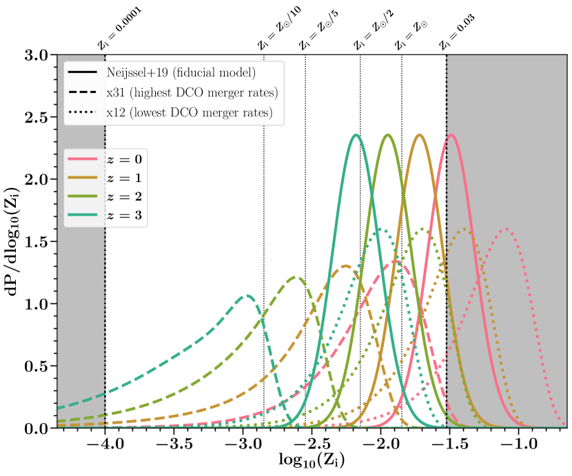
(b)

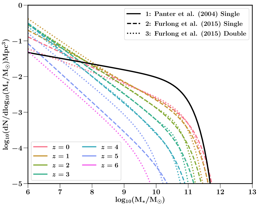
(c)

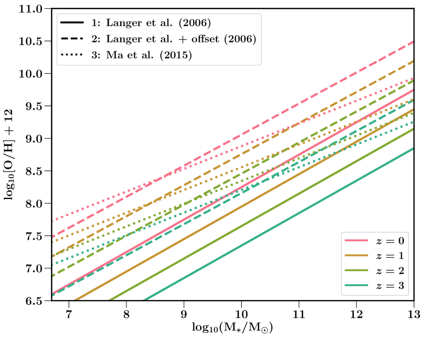
(d)

Figure 16: Figures showing the components that construct the metallicity-specific star formation rate densities (SFRD$(Z_{\rm{i}},z)$) that are used in this study. From left to right and top to bottom we show: (a) the SFRDs, (b) the metallicity distributions $\mathop{}\!\mathrm{d}P/\mathop{}\!\mathrm{d}Z_{\rm{i}}$, (c) the GSMFs and (d) the MZRs. See for more details Table 3 and Section 2.3.

Appendix C Zoom in on Figure 15.

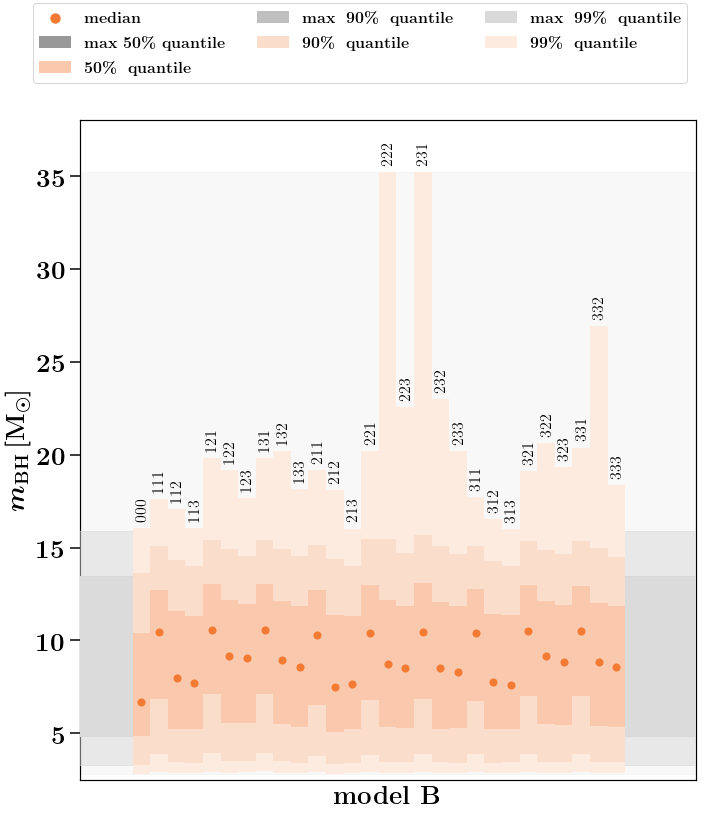
Figure 17: A zoom in of Figure 15 showing the distribution quantiles for the BH mass distribution for all $28$ SFRD$(Z_{\rm{i}},z)$ model variations in combination with the binary population synthesis model B. The figure highlights the SFRD$(Z_{\rm{i}},z)$ bars, adding the SFRD$(Z_{\rm{i}},z)$ label denoted by $\rm{xyz}$ (see Table 3) on top of the corresponding bar. Colored bars from dark to light denote the distribution quantiles for $50\%$, $90\%$ and $99\%$ of the distribution. Scatter points show the median values of the distribution. In the background the maximum range of the $50\%$, $90\%$ and $99\%$ quantiles over all $420$ model variations is shown.

In Figure 17 we give a zoom-in of Figure 15 to show the SFRD$(Z_{\rm{i}},z)$ models that correspond with each bar. The order of the bars, and hence SFRD$(Z_{\rm{i}},z)$ models, is the same throughout all model blocks in Figure 15.

References

- Abadie et al. (2010) Abadie J., et al., 2010, Classical and Quantum Gravity, 27, 173001
- Abbott et al. (2016) Abbott B. P., et al., 2016, Living Reviews in Relativity, 19, 1
- Abbott et al. (2017) Abbott B. P., et al., 2017, Annalen der Physik, 529, 1600209
- Abbott et al. (2018a) Abbott B. P., et al., 2018a, Living Reviews in Relativity, 21, 3
- Abbott et al. (2018b) Abbott B. P., et al., 2018b, Phys. Rev. Lett., 121, 161101
- Abbott et al. (2019) Abbott B. P., et al., 2019, Physical Review X, 9, 031040
- Abbott et al. (2020a) Abbott R., et al., 2020a, arXiv e-prints, p. arXiv:2004.08342
- Abbott et al. (2020b) Abbott B. P., et al., 2020b, Classical and Quantum Gravity, 37, 045006
- Abbott et al. (2020c) Abbott R., et al., 2020c, Phys. Rev. Lett., 125, 101102
- Abbott et al. (2020d) Abbott B. P., et al., 2020d, ApJ, 892, L3
- Abbott et al. (2020e) Abbott R., et al., 2020e, ApJ, 896, L44
- Abbott et al. (2020f) Abbott R., et al., 2020f, ApJ, 900, L13
- Abbott et al. (2021a) Abbott R., et al., 2021a, arXiv e-prints, p. arXiv:2108.01045
- Abbott et al. (2021b) Abbott R., et al., 2021b, Physical Review X, 11, 021053
- Abbott et al. (2021c) Abbott R., et al., 2021c, ApJ, 913, L7
- Abbott et al. (2021d) Abbott R., et al., 2021d, ApJ, 915, L5
- Abt (1983) Abt H. A., 1983, ARA&A, 21, 343
- Abt et al. (1990) Abt H. A., Gomez A. E., Levy S. G., 1990, ApJS, 74, 551
- Acernese et al. (2015) Acernese F., et al., 2015, Classical and Quantum Gravity, 32, 024001
- Ackley et al. (2020) Ackley K., et al., 2020, A&A, 643, A113
- Agrawal et al. (2020) Agrawal P., Hurley J., Stevenson S., Szécsi D., Flynn C., 2020, MNRAS, 497, 4549
- Akmal et al. (1998) Akmal A., Pandharipande V. R., Ravenhall D. G., 1998, Phys. Rev. C, 58, 1804
- Almeida et al. (2017) Almeida L. A., et al., 2017, A&A, 598, A84
- Alsing et al. (2018) Alsing J., Silva H. O., Berti E., 2018, MNRAS, 478, 1377
- Anagnostou et al. (2020) Anagnostou O., Trenti M., Melatos A., 2020, arXiv e-prints, p. arXiv:2010.06161
- Andrews & Mandel (2019) Andrews J. J., Mandel I., 2019, ApJ, 880, L8
- Andrews et al. (2018) Andrews J. J., Zezas A., Fragos T., 2018, The Astrophysical Journal Supplement Series, 237, 1
- Antoniadis et al. (2013) Antoniadis J., et al., 2013, Science, 340, 448
- Arca Sedda (2020) Arca Sedda M., 2020, Communications Physics, 3, 43
- Arca Sedda (2021) Arca Sedda M., 2021, ApJ, 908, L38
- Artale et al. (2019) Artale M. C., Mapelli M., Giacobbo N., Sabha N. B., Spera M., Santoliquido F., Bressan A., 2019, MNRAS, 487, 1675
- Arzoumanian et al. (2002) Arzoumanian Z., Chernoff D. F., Cordes J. M., 2002, ApJ, 568, 289
- Aso et al. (2013) Aso Y., Michimura Y., Somiya K., Ando M., Miyakawa O., Sekiguchi T., Tatsumi D., Yamamoto H., 2013, Phys. Rev. D, 88, 043007
- Asplund et al. (2009) Asplund M., Grevesse N., Sauval A. J., Scott P., 2009, ARA&A, 47, 481
- Astropy Collaboration et al. (2018) Astropy Collaboration et al., 2018, AJ, 156, 123
- Babak et al. (2017) Babak S., Taracchini A., Buonanno A., 2017, Phys. Rev. D, 95, 024010
- Bae et al. (2014) Bae Y.-B., Kim C., Lee H. M., 2014, MNRAS, 440, 2714
- Baibhav et al. (2019) Baibhav V., Berti E., Gerosa D., Mapelli M., Giacobbo N., Bouffanais Y., Di Carlo U. N., 2019, Phys. Rev. D, 100, 064060
- Bailyn et al. (1998) Bailyn C. D., Jain R. K., Coppi P., Orosz J. A., 1998, ApJ, 499, 367
- Banerjee (2020) Banerjee S., 2020, MNRAS,
- Barbieri et al. (2020) Barbieri C., Salafia O. S., Perego A., Colpi M., Ghirlanda G., 2020, European Physical Journal A, 56, 8
- Barkat et al. (1967) Barkat Z., Rakavy G., Sack N., 1967, Phys. Rev. Lett., 18, 379
- Barnes & Kasen (2013) Barnes J., Kasen D., 2013, ApJ, 775, 18
- Barrett et al. (2017) Barrett J. W., Mandel I., Neijssel C. J., Stevenson S., Vigna-Gómez A., 2017, in Brescia M., Djorgovski S. G., Feigelson E. D., Longo G., Cavuoti S., eds, IAU Symposium Vol. 325, Astroinformatics. pp 46–50 (arXiv:1704.03781), doi:10.1017/S1743921317000059
- Barrett et al. (2018) Barrett J. W., Gaebel S. M., Neijssel C. J., Vigna-Gómez A., Stevenson S., Berry C. P. L., Farr W. M., Mandel I., 2018, MNRAS, 477, 4685
- Bavera et al. (2020) Bavera S. S., et al., 2020, A&A, 635, A97
- Bavera et al. (2021) Bavera S. S., et al., 2021, A&A, 647, A153
- Belczynski et al. (2002) Belczynski K., Kalogera V., Bulik T., 2002, ApJ, 572, 407
- Belczynski et al. (2008) Belczynski K., Kalogera V., Rasio F. A., Taam R. E., Zezas A., Bulik T., Maccarone T. J., Ivanova N., 2008, ApJS, 174, 223
- Belczynski et al. (2010a) Belczynski K., Bulik T., Fryer C. L., Ruiter A., Valsecchi F., Vink J. S., Hurley J. R., 2010a, ApJ, 714, 1217
- Belczynski et al. (2010b) Belczynski K., Dominik M., Bulik T., O’Shaughnessy R., Fryer C., Holz D. E., 2010b, ApJ, 715, L138
- Belczynski et al. (2013) Belczynski K., Bulik T., Mandel I., Sathyaprakash B. S., Zdziarski A. A., Mikołajewska J., 2013, ApJ, 764, 96
- Belczynski et al. (2016a) Belczynski K., Holz D. E., Bulik T., O’Shaughnessy R., 2016a, Nature, 534, 512
- Belczynski et al. (2016b) Belczynski K., Repetto S., Holz D. E., O’Shaughnessy R., Bulik T., Berti E., Fryer C., Dominik M., 2016b, ApJ, 819, 108
- Belczynski et al. (2017) Belczynski K., Ryu T., Perna R., Berti E., Tanaka T. L., Bulik T., 2017, MNRAS, 471, 4702
- Belczynski et al. (2020) Belczynski K., et al., 2020, A&A, 636, A104
- Belczynski et al. (2021) Belczynski K., et al., 2021, arXiv e-prints, p. arXiv:2108.10885
- Beniamini & Piran (2016) Beniamini P., Piran T., 2016, MNRAS, 456, 4089
- Beradze et al. (2020) Beradze R., Gogberashvili M., Sakharov A. S., 2020, Physics Letters B, 804, 135402
- Bethe & Brown (1998) Bethe H. A., Brown G. E., 1998, ApJ, 506, 780
- Bhattacharya & van den Heuvel (1991) Bhattacharya D., van den Heuvel E. P. J., 1991, Phys. Rep., 203, 1
- Bhattacharya et al. (2019) Bhattacharya M., Kumar P., Smoot G., 2019, MNRAS, 486, 5289
- Blandford & Teukolsky (1975) Blandford R., Teukolsky S. A., 1975, ApJ, 198, L27
- Blinnikov et al. (1984) Blinnikov S. I., Novikov I. D., Perevodchikova T. V., Polnarev A. G., 1984, Soviet Astronomy Letters, 10, 177
- Boco et al. (2019) Boco L., Lapi A., Goswami S., Perrotta F., Baccigalupi C., Danese L., 2019, ApJ, 881, 157
- Boco et al. (2021) Boco L., Lapi A., Chruslinska M., Donevski D., Sicilia A., Danese L., 2021, ApJ, 907, 110
- Bouffanais et al. (2021) Bouffanais Y., Mapelli M., Santoliquido F., Giacobbo N., Iorio G., Costa G., 2021, MNRAS, 505, 3873
- Brandt et al. (1995) Brandt W. N., Podsiadlowski P., Sigurdsson S., 1995, MNRAS, 277, L35
- Breivik et al. (2020) Breivik K., et al., 2020, ApJ, 898, 71
- Brisken et al. (2002) Brisken W. F., Benson J. M., Goss W. M., Thorsett S. E., 2002, ApJ, 571, 906
- Broekgaarden & Berger (2021) Broekgaarden F. S., Berger E., 2021, arXiv e-prints, p. arXiv:2108.05763