Microscopic theory of pygmy- and giant resonances:
Accounting for complex 1p1h$\otimes$phonon and two-phonon configurations

Abstract

The self-consistent Theory of Finite Fermi Systems (TFFS) is consistently generalized for the case of accounting for phonon coupling (PC) effects in the energy region of pygmy- and giant multipole resonances (PDR and GMR) in magic nuclei with the aim to consider particle-hole (ph) and both complex 1p1h$\otimes$phonon and two-phonon configurations. The article is the direct continuation and generalization of the previous article [S.Kamerdzhiev, M.Shitov, Eur.Phys.J.A. 56, 265 (2020)], referred to as [I], where 1p1h- and only complex 1p1h$\otimes$phonon configurations were considered. The newest equation for the TFFS main quantity, the effective field (vertex), which describes the nuclear polarizability, has been obtained. It has considerably generalized the results of the previous article and accounts for two-phonon configurations. Two variants of the newest vertex equation have been derived: (1)the first variant contains complex 1p1h$\otimes$phonon configurations and the full 1p1h-interaction amplitude $\Gamma$ instead of the known effective interaction F in [I], (2) the second one contains both 1p1h$\otimes$phonon and two-phonon configurations. Both variants contain new, as compared to usual approaches, PC contributions, which are of interest in the energy region under consideration and, at least, should result in a redistribution of the PDR and GMR strength, which is important for the explanation of the PDR and GMR fine structure. The qualitative analysis and discussion of the new terms and the comparison to the known time-blocking approximation are performed.

I Introduction

The experimental and theoretical studies of multipole pygmy-and giant resonances, especially pygmy-dipole resonance (for simplicity, hereinafter PDR and GMR), continue to draw much attention, see reviews Savran ; Paar ; Bracco ; revKST ; kaevYadFiz2019 . For PDR , it is explained by the new experimental possibilities Cosel ; Larsen ; Bracco , for example, polarized proton inelastic scattering at very forward angles Cosel , the existence of many new and delicate physical effects in this energy region, like irrotational and vortical kind of motion Nester ; Paar and the upbend phenomenon for the photon strength function in the energy region of 1-3 MeV Larsen . Besides, as it turned out, it is impossible to explain completely, with the account of phonon coupling (PC), the observed PDR fine structure, even in the nucleus ²⁰⁸Pb, within both non-self-consistent rezaeva and self-consistent Lyutor2018 approaches.

From a physical point of view, the problem is understandable, but only in principle: it is necessary to take into account the phonon coupling (PC) effects in addition to the standard random phase approximation (RPA) and quasiparticle RPA (QRPA) approaches. Here, several non-self-consistent and self-consistent approaches have been developed, see reviews Paar ; Bracco ; kaevYadFiz2019 , which considered both 1p1h$\otimes$phonon and 1p1h$\otimes$phonon + two-phonon configurations. But they still have room for the improvement. We are sure that the use of consistent quantum many-body formalism, to be more exact, the Green function (GF) method, including generalization of the self-consistent Theory of Finite Fermi Systems (TFFS) Migdal ; KhSap1982 is very promising for further work.

In the self-consistent TFFS, which was developed in KhSap1982 and partly described in the second edition of Migdal’s book Migdal2 , it was shown that in all the numerous problems considered kaevYadFiz2019 PC contributions were considerable, of fundamental importance and necessary for explaining experimental data. In the works KhSap1982 only the self-consistent description of characteristics of the ground and low-lying collective states was considered. The success of these works is explained, first of all, by a more consistent consideration of PC effects, in particular, the tadpole effects KhSap1982 ; SapTol2016 and, probably, by the effect of the effective interaction variation in the phonon field voitenkov .

In our opinion, the next natural step is to go further and to consider the field of PDR + GMR within the self-consistent TFFS. This is the general aim of our article

The theory for PDR and GMR was developed, within the GF method and with PC, in the framework of both non-self-consistent kaev83 ; ts89 ; revKST and self-consistent variants ts2007 ; ave2011 . The difference between kaev83 and ts89 consisted in the fact that in ts89 the disadvantage of kaev83 was eliminated, namely, a special approximate method of chronological decoupling of diagrams (MCDD) (or, in a more modern terminology, time blocking approximation (TBA)) was developed in order to solve the problem of second-order poles in the generalized propagator of the extended RPA propagator in kaev83 . This disadvantage was not important for explanation of the properties of M1 resonance ktZPhys ; kt1984 , which is in the PDR energy region. Moreover, earlier it was even used within Nuclear Field Theory (NFT) for electrical GMR Bortignon ; Bortignon2 with the smearing parameter of 600 keV. Later on, this method to solve the second-order poles problem was considerably improved ts2007 so that the approach obtained the name of quasiparticle time blocking approximation (QTBA) for nuclei with pairing and TBA for magic nuclei, respectively. TBA and QTBA and their modifications have been applied for the description of PDR and also GMR in magic and semi-magic nuclei ts2018 ; litva-schuck ; Larsen ; kaev2014 . Usually, in the most part of these works the calculations were performed with the use of a smearing parameter, which was taken to be equal to the experimental resolution of about 100-500 keV. However, the main physical content, i.e. inclusion of PC only into the particle-hole (ph) propagator (in the language of TFFS) was always preserved despite the fact that the derivation method was different and was based on the Bethe-Salpeter equation. Unfortunately, even the known tadpole effect was not considered in the generalized propagator of MCDD, or TBA.

In article KaShi , which further will be referred to as [I], a theory of PDR and GMR was developed within the GF method in the approximation of 1p1h+1p1h$\otimes$phonon configurations. The consistent generalization of the standard TFFS with the aim to include $g^{2}$ PC corrections, where $g$ is the creation amplitude of the usual RPA phonon, allowed us to obtain new PC contributions to the new equation for the main TFFS quantity - vertex V. They included the dynamical tadpole effects for the vertex, the so-called induced interactions caused by the phonon exchange and the first and second variations of the effective interaction in the phonon field. In article [I], we used the approximation for the first and second variations of the vertex V in the phonon field, namely, only free terms of the equations for them were used, which provided accounting for only complex 1p1h$\otimes$phonon configurations. In the present article, we reject this approximation and consider the exact equations for the vertex variations, i.e. accurate expressions obtained for them.

The restriction by only complex 1p1h$\otimes$phonon configurations is not enough in the PDR+GMR field, at least for the explanation of the PDR fine structure. In the non-self-consistent approaches, this can be seen from numerous calculations in the PDR energy region, see Savran ; rezaeva , performed within the non-self-consistent Quasiparticle-Phonon Model (QPM) Sol89 . In order to improve the agreement with the $(e,e^{\prime})$-experiments there, it was necessary to add more complex, first of all, two-phonon configurations. As it was said earlier, the comparison to the latest experimental results obtained with polarized proton inelastic scattering at very forward angles Cosel , also confirmed that, within the self-consistent approaches with only 1p1h$\otimes$phonon configurations Lyutor2018 , it was not possible to explain the PDR fine structure in ²⁰⁸Pb. The importance of the role of two-phonon configurations in this problem was also underlined in self-consistent calculations of it-z2015 .

The goal of this article is to do the next necessary and essential step further than in article [I]. Namely, to analyse the consequences of the use of accurate expressions for the first and second variations of the vertex in the phonon field instead of the approximate ones, and, as one of these consequences, to add the second type of complex configurations, i.e., two-phonon ones.

In this article, we will consider only magic nuclei, complex 1p1h$\otimes$phonon and two-phonon configurations. As usual, we use the fact of existence of the small $g^{2}$ parameter. Very often we symbolically write our formulas, the main of which are represented in the form of Feynman diagrams, so the final formulas can be easily obtained.

II Some earlier results

II.1 Some initial formulas of TFFS.

In the standard TFFS, the main quantity in the problems connected with the interaction between a nucleus and an external field $V^{0}(\omega)$ with the energy $\omega$, is the notion of effective field (vertex) $V$, which describes the nuclear polarizability and satisfies the equation in the symbolic form Migdal :

$$V=e_{q}V^{0}+FAV,$$ (1)

where the ph-propagator reads:

$$A_{12}(\omega)=\int G_{1}(\varepsilon)G_{2}(\varepsilon-\omega)d\varepsilon.$$ (2)

The full 1p1h-interaction amplitude $\Gamma(\omega)$ satisfies the equation:

$$\Gamma=F+FA\Gamma$$ (3)

In Eq.(1) and Eq.(3), F is the effective interaction, which in the self-consistent TFFS is calculated as the second variational derivative of the energy density functional and the mean field is calculated as the first variational derivative of the energy density functional. Low indices mean a set of single-particle quantum numbers 1 $\equiv({n_{1},j_{1},l_{1},m_{1}})\equiv\lambda_{1}$ and we write $d\varepsilon$ instead of $\frac{d\varepsilon}{2\imath\pi}$ everywhere.

The phonon creation amplitude g satisfies the equation Migdal

$$g=FAg.$$ (4)

Eq.(1), Eq.(3) and Eq.(4) comply with the RPA approach written in the FG language, i.e. with the standard TFFS. We will use them as the initial relations or input data for further development. And we will speak about generalization of the standard TFFS just in this sense in the present article.

II.2 Earlier results with PC

As it was mentioned in the Introduction, the physical content of the previous GF approaches in the PDR and GMR theory consisted in the fact that $g^{2}$ PC corrections were included only into ph-propagator, Eq.(2). So, in the language of TFFS, the diagrams presented in Fig.1 should correspond to the equation for the vertex $V^{\prime}$ with the simplest PC ph-propagator. The case without the MCDD prescription was realised in kaev83 ; kt1984 ; ktZPhys for M1 resonances in magic nuclei. Physically, they also correspond to the approach within NFT Bortignon ; Bortignon2 for GMR.

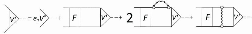
Figure 1: Equation for the vertex $V^{\prime}$ containing the simplest ph-propagator with PC kaev83 ; ktZPhys . Straight and wavy lines correspond to GFs G and D, circles with one wavy line stand for the amplitude of phonon production g. The rectangle stands for the effective interaction F. See text for details.

In Fig.1 the diagrams without phonons represent the RPA case for the vertex V formulated in the standard TFFS language, Eq.(1), with the ph-propagator A, Eq.(2). Hereinafter, number 2 before a graph or a corresponding formula means that there are two graphs or formulas of a similar type. Of course, it is necessary to keep in mind that in reality the MCDD prescription ts89 , or TBA, should be used for numerical results to avoid the above-mentioned problem with the second-order poles in the PC propagator shown in Fig.1. Such a generalized MCDD propagator is rather complicated, it was discussed in details and given in revKST .

In the works performed within the self-consistent TFFS, the $g^{2}$ PC corrections to the mean field, which take into account the tadpole, were actively used. They can be written in the symbolic form as

$$\delta\Sigma=gDGg+g_{11}D$$ (5)

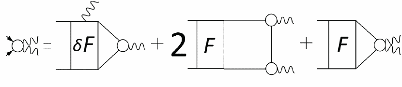
Figure 2: Diagram representation of Eq.(7). The circle with two wavy lines is $g_{12}$, which (with 1=2) is contained in the tadpole

Here $\Sigma$ is the self-energy operator, G and D are the single-particle and phonon GF’s:

$$G_{1}(\varepsilon)=\frac{1-n_{1}}{\varepsilon-\varepsilon_{1}+\imath\gamma}+\frac{n_{1}}{\varepsilon-\varepsilon_{1}-\imath\gamma},$$

$$D_{s}(\omega)=\frac{1}{\omega-\omega_{s}+\imath\gamma}-\frac{1}{\omega+\omega_{s}-\imath\gamma},$$ (6)

g obeys the homogeneous equation (4) and $\varepsilon_{1}\equiv\varepsilon_{\lambda_{1}},n_{1}\equiv n_{\lambda_{1}}$

The amplitude of creation of two phonons, similar in the tadpole case, is obtained as the variation of Eq.(4) in the field of the phonon 2

$$g_{12}\equiv\delta^{(1)}g_{2}=\delta^{(1)}FAg_{2}+F\delta^{(1)}Ag_{2}+FAg_{12}$$ (7)

This equation shown in Fig.2 was solved only in the coordinate representation in the works pertaining to other problems connected with the properties of the ground or low-lying collective states platonov ; KhSap1982 . In the works of Kurchatov Institute group KhSap1982 ; SapTol2016 , a realistic estimation of the two-phonon creation amplitude $g_{11}\equiv\delta^{(1)}g_{1}$ contained in the phonon tadpole term $K^{ph}=\int d\omega g_{11}D$ was used. This estimation was based on the ansatz for the quantity $\delta F$ KhSap1982 :

$$\delta F=(\raisebox{1.0pt}{$\delta F$}\big{/}\raisebox{-1.0pt}{$\delta\rho$})\,Ag$$ (8)

III Exact expressions for first and second variations of the vertex $\delta V$ and $\delta^{(2)}V$

In order to obtain the full $g^{2}$ corrections to the vertex V, Eq.(1), we will use, like in [I], the following expressions for them

$$\tilde{V}=V+\Delta V(g,V)$$ (9)

and

$$\Delta V=2gDG\delta^{(1)}V+\delta^{(2)}VD,$$ (10)

where the quantities $\delta^{(1)}V$ and $\delta^{(2)}V$ are the first- and second-order variations of the vertex $V$, Eq.(1), in the phonon field. These corrections are shown in Fig.3.

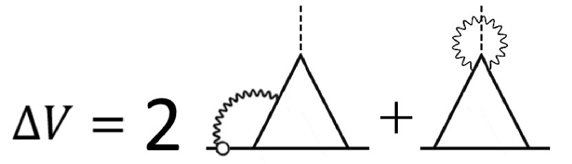
Figure 3: The $g^{2}$ corrections to the vertex V, Eq.(10)

The second term in Eq.(10), Fig.3, contains ”pure” $g^{2}$ corrections, while the first term in Eq.(10), Fig.3, is a mix of the first-order correction to the vertex $V$ and the ”end” corrections of the first order in $g$.

First of all, let us obtain the quantity $\delta^{(2)}A$ contained in $\delta^{(2)}V$ for our case of similar phonons. In order not to confuse it with the single-particle index 1, here we introduce the notion $\tilde{1}$ for the phonon 1. When $\tilde{1}=\tilde{2}$, which is of interest in our case of the variation $\delta^{(2)}V=\delta^{\tilde{1}}\delta^{\tilde{1}}V$, we obtain five terms (instead of eight in the general case of unequal phonons for $g_{\tilde{1}\tilde{2}}$); they are shown in Fig.4.

$$\delta^{(2)}A=\delta^{\tilde{1}}\delta^{\tilde{1}}G_{1}G_{2}=2G_{1}g_{\tilde{1}}G_{4}g_{\tilde{1}}G_{3}G_{2}+$$

$$2G_{1}g_{\tilde{1}\tilde{1}}G_{3}G_{2}+G_{1}g_{\tilde{1}}G_{3}G_{2}g_{\tilde{1}}G_{4}$$ (11)

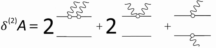
Figure 4: Expression (11) in the diagrammatic representation.

The quantities $\delta^{(1)}V$ and $\delta^{(2)}V$ are obtained by variation of Eq.(1) in the phonon field:

$$\delta^{(1)}V= \delta^{(1)}FAV+F\delta^{(1)}AV+FA\delta^{(1)}V,$$

$$\delta^{(2)}V= \delta^{(1)}\delta^{(1)}V=F\delta^{(2)}AV+$$

$$2\delta^{(1)}F\delta^{(1)}AV+2\delta^{(1)}FA\delta^{(1)}V+2F\delta^{(1)}A\delta^{(1)}V+$$

$$\delta^{(2)}FAV+FA\delta^{(2)}V$$ (12)

In [I] the quantities $\delta^{(1)}V$ and $\delta^{(2)}V$ were accounted approximately; namely, only free terms of equations Eq.(12) were taken into account for them. This approximation provided accounting for only 1p1h$\otimes$phonon configurations.

In this article, we reject this approximation. We transform the obtained equations Eq.(12)for $\delta^{(1)}V$ and $\delta^{(2)}V$ to the expressions for $\delta^{(1)}V$ and $\delta^{(2)}V$ without loss of accuracy. Note that we use Eq.(4), i.e. the RPA (or TFFS) approach, for phonons.

Let us rewrite the equations for $\delta^{(1)}V$ and $\delta^{(2)}V$ as follows:

$$\delta^{(1)}V=(\delta^{(1)}V)_{0}+FA\delta^{(1)}V,$$

$$\delta^{(2)}V=(\delta^{(2)}V)_{0}+FA\delta^{(2)}V,$$ (13)

where $(\delta^{(1)}V)_{0}$ and $(\delta^{(2)}V)_{0}$ are free terms of Eq.(12). In the other form, we have (symbolically as always):

$$(1-FA)\delta^{(1)}V=(\delta^{(1)}V)_{0},$$

$$(1-FA)\delta^{(2)}V=(\delta^{(2)}V)_{0},$$ (14)

or

$$\delta^{(1)}V=(1-FA)^{-1}(\delta^{(1)}V)_{0}$$

$$\delta^{(2)}V=(1-FA)^{-1}(\delta^{(2)}V)_{0}.$$ (15)

Following Khodel , we introduce also the quantity d$\Gamma$ (to avoid mixing with the usual variation of Eq.(3), we redefined it instead of $\delta\Gamma$ in Khodel )

$$d\Gamma=\delta^{(1)}F+FAd\Gamma.$$ (16)

Further we will use the following symbolic expressions obtained from Eq.(3) and Eq.(16)

$$\Gamma=(1-FA)^{-1}F$$

$$d\Gamma=(1-FA)^{-1}\delta^{(1)}F$$ (17)

Substituting the free terms $(\delta^{(1)}V)_{0}$ and $(\delta^{(2)}V)_{0}$ of Eq.(12) into Eq.(15) and using Eqs.(17), we obtain the accurate expressions for $\delta^{(1)}V$ and $\delta^{(2)}V$:

$$\delta^{(1)}V=d\Gamma AV+\Gamma\delta AV$$

$$\delta^{(2)}V=\Gamma\delta^{(2)}AV+2d\Gamma\delta AV+2d\Gamma A\delta V+$$

$$2\Gamma\delta A\delta V+d^{(2)}\Gamma AV,$$ (18)

which contain $\Gamma$ and $d\Gamma$ instead of F and $\delta F$ and we have introduced a new quantity

$$d^{(2)}\Gamma=\delta^{(2)}F+FAd^{(2)}\Gamma,$$ (19)

or

$$d^{(2)}\Gamma=(1-FA)^{-1}\delta^{(2)}F.$$ (20)

The obtained exact expressions for $\delta^{(1)}V$ and $\delta^{(2)}V$ are shown in Fig.5. Note, the ”accuracy” for $\delta^{(1)}V$ and $\delta^{(2)}V$ consists in the fact that they contain just the TFFS equations for vertex V, Eq.(1), amplitude $\Gamma$, Eq.(3), phonon creation amplitude $g$ Eq.(4) and $d\Gamma$, Eq.(16), i.e. in this sense everything is completely within the initial ideas of the standard TFFS Migdal . The principal difference from [I] is that now we use the accurate expressions for $\delta^{(1)}V$ and $\delta^{(2)}V$, Fig.5, instead of free terms of Eq.(12) for them.

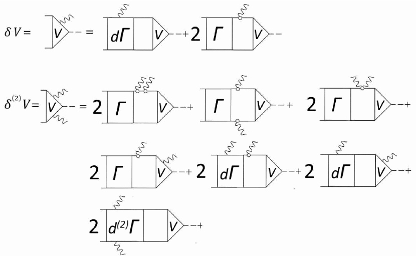
Figure 5: Exact expressions, Eq.(18), for the first and second variations of the vertex V $\delta^{(1)}V$ and $\delta^{(2)}V$ in the phonon field. The boxes with $\Gamma$, $d\Gamma$ and $d^{(2)}\Gamma$ stand for quantities $\Gamma$, Eq.(3), $d\Gamma$, Eq.(16) and $d^{(2)}\Gamma$, Eq.(19), respectively.

IV The newest equation for the effective field

IV.1 1p1h$\otimes$phonon configurations and the full interaction amplitude $\Gamma$

Let us go back to expression (9). One can see that expression (9) is the first iteration of the following equation (if $V$, Eq.(1), is zero iteration)

$$\tilde{V}=V+\Delta V(g,\tilde{V}),$$ (21)

where $\Delta V(g,\tilde{V})$ contains the newest vertex $\tilde{V}$ in the quantities $\delta^{(1)}V$ and $\delta^{(2)}V$ of Eq.(18). Using Eq.(1) and Eq.(21) one can obtain

$$\tilde{V}=V^{0}+FA\tilde{V}+(1-FA)\Delta V(g,\tilde{V}).$$ (22)

Let us substitute into Eq.(22) the exact expressions for $\delta^{(1)}V$ and $\delta^{(2)}V$, Eq.(18) (which already contain $\tilde{V}$) and use the relations (17) and (20). After a long derivation with the use of footnote 1 on page 2, four terms are cancelled and, as the result, the following equation for $\tilde{V}$ is obtained:

$$\tilde{V}=e_{q}V^{0}+FA\tilde{V}+2FGgDGgGG\tilde{V}+FGgGDGgG\tilde{V}+$$

$$2FGg_{\tilde{1}\tilde{1}}DGG\tilde{V}+4gGD\Gamma GgGG\tilde{V}+$$

$$2gDGd\Gamma GG\tilde{V}+2\delta FDGgGG\tilde{V}+$$

$$2\delta FDGG\Gamma GgGG\tilde{V}+$$

$$\delta FDGGd\Gamma GG\tilde{V}+\delta^{(2)}FGG\tilde{V}$$ (23)

This equation contains 10 integral terms instead of 12 in Eq.(16),[I] (note that in the analytic form of the equation we write digit 4 in the second line of Eq.(23) instead of digit 2 in graphic representation of two similar graphs). Eq.(23) can be easily represented in a graphic form. However, for our aim to include two-phonon configurations (see the next section), it is better to work not with the quantities $d\Gamma$ in Eq.(23) but with the amplitudes $\Gamma$. So, for it, we transform the equation for $d\Gamma$, Eq.(16), to the expression, which contains the amplitude $\Gamma$:

$$d\Gamma=\delta F+\Gamma A\delta F=\delta F+\Gamma GG\delta F.$$ (24)

Then, substituting Eq.(24) into Eq.(23), we obtain the equation for $\tilde{V}$, which contains only $\delta F$ and $\Gamma$:

$$\tilde{V}=e_{q}V^{0}+FA\tilde{V}+2FGgDGgGG\tilde{V}+FGgGDGgG\tilde{V}+$$

$$2FGg_{\tilde{1}\tilde{1}}DGG\tilde{V}+4gGD\Gamma GgGG\tilde{V}+$$

$$2gDG\delta FGG\tilde{V}+2gDG\Gamma GG\delta FGG\tilde{V}+2\delta FDGgGG\tilde{V}+$$

$$2\delta FDGG\Gamma GgGG\tilde{V}+$$

$$\delta FDGG\delta FGG\tilde{V}+\delta FDGG\Gamma GG\delta FGG\tilde{V}+\delta^{(2)}FGG\tilde{V},$$ (25)

It is shown in Fig.6. .

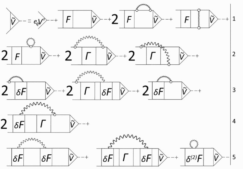
Figure 6: Graphic representation of Eq.(25)

Eq.(25), Fig.6, contains only known quantities $\Gamma$, $g$ and $g_{11}$, which satisfy Eq.(3), Eq.(4) and Eq.(7), respectively. The quantity $\delta F$ can be estimated with the use of ansatz in Eq.(8). Thus, Eq.(25), Fig.6, is the first main result of our article. It is exact in the sense that here we have used the exact expressions Eq.(18) for the first and second variations $\delta^{(1)}V$ and $\delta^{(2)}V$ of the vertex V, Eq.(1), in the phonon field.

This is a noticeable generalization of Eq.(16), Fig.6, in article [I]. Let us compare our Eq.(25), Fig.6, and Eq.(16), Fig.6, of [I]. For simplicity, we enumerate the terms of Eq.(25), Fig.6, in accordance with their lines as follows:

$$\tilde{V}=\tilde{V}^{1}+\tilde{V}^{tad}+\tilde{V}^{2}_{n}+\tilde{V}^{3}_{n}+\tilde{V}^{4}_{n}+\tilde{V}^{5}_{n}$$ (26)

Here the upper indices mean only the number of the line in Eq. (25), Fig.6. Some parts of Eq.(26) may include two or three terms in each line (with digit 2 each). Low index n in four terms of Eq.(26) shows that these terms contain new terms as compared to [I].

1. We obtained the full coincidence with [I] in line 1 and for the first term of line 2 (the dynamical effect of the tadpole)

2. However, there are considerable differences. Namely, while Eq.(16), Fig.6, in [I] contains the effective interaction F and $\delta F$, in our case five terms with the full amplitude $\Gamma$ appear. It gives the possibility to obtain naturally two-phonon configurations (see the next section). In the terms $\tilde{V}^{2}_{n}$ of line 2 we obtained the terms similar to [I], but, what is of most interest, in our case they contain the full amplitude $\Gamma$, instead of the effective interaction $F$ in the same terms in [I]. $\Gamma$ is not a static quantity and depends on the energy $\omega$. In this sense, these four terms are physically similar to the results in litva-schuck shown in Fig.13 of litva-schuck . However, in contrast to litva-schuck , here we cannot include the configurations more complex than two-phonon ones. The reason is that in our case it would be incorrect to go beyond the formulas in Section II.A.

All the terms in lines 3,4,5 of Eq.(25), Fig.6, are new as compared to TBA and other models and methods in the PDR and GMR field because they contain $\delta F$, and, among them, there are three terms with $\Gamma$ in lines 3,4,5.

IV.2 1p1h$\otimes$phonon and two-phonon configurations

To obtain all previous results, i.e. to generalize TFFS for the PC case, we have used the initial TFFS formulas described in Section II.A. In order to preserve the consistency of this approach for the inclusion of two-phonon configurations, it is also necessary to use TFFS. And Eq.(25) gives such a possibility. Let us consider the expansion in phonons for the amplitude $\Gamma$

$$\Gamma(\omega)=\sum_{s}\frac{g^{s}g^{s*}}{\omega-\omega_{s}},$$ (27)

where $g$ satisfies Eq.(4). In the PDR and GMR calculations, as a rule, a great number of phonons are used, so that the expansion in phonons, Eq.(27), exhausts almost all $\Gamma$. Making use of the RPA phonons for accounting for PC effects is applied in many modern approaches, like QPM Sol89 , TBA and QTBA ts2007 , relativistic QTBA litva-ring-ts . We will see that our approach for the TFFS generalization gives some additional effects.

In principle, in Eq.(27), one could add a regular part $\Gamma^{r}$ that does not depend on $\omega$. However, such an approach will give a strong complication. First, a necessity to find $\Gamma^{r}$. Second, one can easily obtain that the use of $\Gamma^{r}$ will strongly complicate the equation for $\tilde{V}$. Indeed, in this case, the quantity $\Gamma^{r}$ will appear in line 2 of Fig.6 and in other lines containing $\delta F$. These new terms will generalize the results of [I] in such a way that the new quantities $\Gamma^{r}_{ind}$, which differ from $F_{ind}$ in [I] only by F changed by an unknown quantity $\Gamma^{r}$, should be in line 2 of Fig.6 and in other lines. Such a complication is not constructive at this stage and will be discussed somewhere else. For these reasons, in this article we omit $\Gamma^{r}$. Substituting Eq.(27) into the term $2gDGg\Gamma G$, which plays the role of a phonon-induced interaction, we have (symbolically):

$$gDG\Gamma Gg=gGgDDgGg,$$ (28)

which is shown in a graphic form in Fig.7. However, note that, for example, for the problems with consideration of two specific phonons, in principle, it will be necessary to find $\Gamma^{r}$.

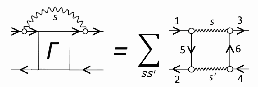
Figure 7: Graphic representation of Eq.(28).

In order to obtain the final newest equation for the vertex $\tilde{V}$, it is necessary to substitute Eq.(27) into all five terms of Eq.(25), Fig.6, which contain the amplitude $\Gamma$. The result is as follows:

$$\tilde{V}=e_{q}V^{0}+FA\tilde{V}+2FGgDGgGG\tilde{V}+FGgGDGgG\tilde{V} +$$

$$2FGg_{\tilde{1}\tilde{1}}DGG\tilde{V}+$$

$$4gGgDDgGgGG\tilde{V}+$$

$$2g\delta FDGGG\tilde{V}+2\delta FDGgGG\tilde{V}+$$

$$2\delta FDGG\delta FGG\tilde{V}+\delta^{(2)}FDGG\tilde{V}+$$

$$\delta FGGgDDgGG\delta FGG\tilde{V}+$$

$$2gGgDDgGG\delta FGG\tilde{V}+$$

$$2\delta FGGgDDgGgGG\tilde{V}$$ (29)

It is shown in Fig.8. The lines of Eq.(29) and Fig.8 correspond to each other. Due to the symbolical form of Eq.(29), in line 3, we have shown two graphs in Fig.8 instead of the terms with digit 4 in the same line 3 of Eq.(29)

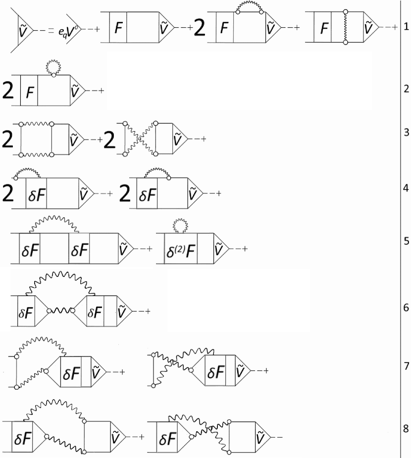
Figure 8: Graphic representation for Eq.(29)

Using the standard diagram technique, one can easily see that Eq.(29), Fig.8, contains both 1p1h$\otimes$phonon configurations in all the lines, except for the RPA part (Eq.(1)) in line 1, and two-phonon configurations in lines 3, 6, 7, 8. Thus, Eq.(29), Fig.8, is the second main result of our article.

V Discussion of the newest equation for the effective field $\tilde{V}$

V.1 General description.
Comparison to article [I]

In subsections A and B of the previous Section IV, Fig.6 and Fig.8, respectively, we obtained the justification of our ansatz in [I], where the very first integral term $FA\tilde{V}$ was included intuitively instead of $FAV$. This justification is due to inclusion of the exact expressions for $\delta^{(1)}V$ and $\delta^{(2)}V$.

Like in [I] and also in the case of 1p1h$\otimes$phonon configuration in the previous section, see Eq.(25), Fig.6, we obtained the full coincidence with [I] in line 1 and in the first term of line 2 (the dynamical tadpole effect). Besides, this is a considerable generalization of Eq.(16), Fig.6, in article [I]. As compared to Eq.(16), Fig.6 of [I], we obtained new five terms with two-phonon configurations in lines 3, 6, 7, 8 in Eq.(29).

All the terms in lines 4, 5, 6, 7, 8 of Eq.(29), Fig.8, are quite new as compared to TBA and other models and methods in the PDR and GMR field because they contain $\delta F$.

For simplicity, we enumerate the terms of Eq.(29), Fig.8, in accordance with their lines as follows:

$$\tilde{V}=\tilde{V}^{1}+\tilde{V}^{tad}+\tilde{V}^{3}_{2phon}$$

$$+\tilde{V}^{4}+\tilde{V}^{5}++\tilde{V}^{6}_{2phon}+\tilde{V}^{7}_{2phon}+\tilde{V}^{8}_{2phon}$$ (30)

Here the upper indices 1-8 mean only the number of the line in Eq.(29), Fig.8. The low indices $2phon$ mean that the terms contain two-phonon configurations. Some parts of Eq.(30) may include two terms in each line.

1. We obtained the full coincidence between Eq.(16), Fig.6[I], and Eq.(29), Fig.8, in lines 1 and lines 2 (the dynamical effect of the tadpole). See the discussion about these terms in Section 4 in [I].

2. Four terms in lines 4 and 5, $\tilde{V}^{4}$ and $\tilde{V}^{5}$, coincide with $\tilde{V}^{4}$ and $\tilde{V}^{6}$ in [I], respectively, they were obtained and discussed there. They are of order $g^{2}$.

3. The terms in lines 6, 7, 8, i.e. $\tilde{V}^{6}_{2phon},\tilde{V}^{7}_{2phon}$ and $\tilde{V}^{8}_{2phon}$, contain two-phonon configurations and $(\delta F)^{2}g^{2}$, $(g^{3}\delta F)$ and $(\delta F)g^{3}$, respectively. Since $\delta F$ contains g, see Eq.(8), all these terms are of order $g^{4}$.

All the terms in lines 4-8 contain the quantity $\delta F$ , $(\delta F)^{2}$ or $\delta^{(2)}F$. The quantity $\delta F$ is expressed in terms of the three-quasiparticle effective interaction amplitude $W$ KhSap1982 :

$$\delta_{s}F=WGg_{s}G.$$ (31)

As the role of this interaction is known to be small on the whole, one can think that the terms with $\delta F$ will give a small contribution. We have only one real example when it was estimated numerically voitenkov with the use of Eq.(8): the contribution of the term with $\delta F$ was very small for the case of static characteristics. So, in the present article, we will not consider these lines and further down we will consider only terms $\tilde{V}^{3}_{2phon}$, see Section B. We will obtain general formulas for them, but, first of all, and in a more detailed form, we consider quite new phonon-induced interactions that appear in line 3, which are caused by the phonon exchange in various channels (ph, hp, pp, hh).

V.2 Terms $\tilde{V}^{3}_{2phonon}$ (line 3). Two-phonon configurations.
Comparison to the TBA model.

Here we introduce the two-phonon induced interaction $F^{2phonon}_{ind}$ for the first of the two two-phonon graphs of Fig.8:

$$(F^{2phonon}_{ind})_{1234\_1}(\varepsilon_{1},\varepsilon_{3},\omega)=$$

$$\sum_{56ss^{\prime}}g^{s}_{15}g^{s*}_{63}g^{s^{\prime}}_{52}g^{s^{\prime}*}_{46}I_{56ss^{\prime}\_1}\delta(\varepsilon_{1}-\varepsilon_{2}+\varepsilon_{4}-\varepsilon_{3}),$$ (32)

$$I_{56ss^{\prime}\_1}(\varepsilon_{1},\varepsilon_{3})=$$

$$\int G_{5}(\varepsilon_{1}-\omega_{1})G_{6}(\varepsilon_{3}-\omega_{1})D_{s}(\omega_{1})D_{s^{\prime}}(\omega_{1}-\omega)d\omega_{1}.$$ (33)

The first two-phonon induced interaction $F^{2phonon}_{ind}$, which is present in the second (”crossed”) graph of line 3, Fig.(8), reads:

$$(F^{2phonon}_{ind})_{1234\_2}(\varepsilon_{1},\varepsilon_{4},\omega)=$$

$$\sum_{56ss^{\prime}}g^{s}_{15}g^{s*}_{46}g^{s^{\prime}}_{52}g^{s^{\prime}*}_{63}I_{56ss^{\prime}\_2}\delta(\varepsilon_{1}-\varepsilon_{2}+\varepsilon_{4}-\varepsilon_{3}),$$ (34)

$$I_{56ss^{\prime}\_2}(\varepsilon_{1},\varepsilon_{4})=$$

$$\int G_{5}(\varepsilon_{1}-\omega_{1})G_{6}(\varepsilon_{4}+\omega_{1})D_{s}(\omega_{1})D_{s^{\prime}}(\omega_{1}-\omega)d\omega_{1}.$$ (35)

The results of integration in Eq.(33) and Eq.(35) are given in Eq.(36), where we introduced $(\varepsilon_{1}-\varepsilon_{2})=(\varepsilon_{3}-\varepsilon_{4})=\omega$. Eq.(36) was obtained with the help of computer transformations from the initial much more cumbersome results of integrations in order to try and single out (unsuccessfully !) only terms with $[\omega\pm(\omega_{s}+\omega_{s}^{\prime})]^{-1}$.

$$I_{56ss^{\prime}\_1}(\varepsilon_{1},\varepsilon_{3},\omega)=$$

$$\frac{1-n_{\lambda_{5}}}{(\varepsilon_{3}+\varepsilon_{\lambda_{5}}-\varepsilon_{\lambda_{6}}-\varepsilon_{1})(\varepsilon_{1}-\varepsilon_{\lambda_{5}}-\omega_{s})(\varepsilon_{1}-\varepsilon_{\lambda_{5}}-\omega-\omega_{s}^{\prime})}-\frac{n_{\lambda_{5}}}{(\varepsilon_{3}+\varepsilon_{\lambda_{5}}-\varepsilon_{\lambda_{6}}-\varepsilon_{1})(\varepsilon_{1}-\varepsilon_{\lambda_{5}}+\omega_{s})(\varepsilon_{1}-\varepsilon_{\lambda_{5}}-\omega+\omega_{s}^{\prime})}+$$

$$\frac{(1-n_{\lambda_{5}})n_{6}}{(\varepsilon_{3}+\varepsilon_{\lambda_{5}}-\varepsilon_{\lambda_{6}}-\varepsilon_{1})(\varepsilon_{3}-\varepsilon_{\lambda_{6}}+\omega_{s})(\varepsilon_{3}-\varepsilon_{\lambda_{6}}-\omega+\omega_{s}^{\prime})}-\frac{n_{\lambda_{5}}(1-n_{6})}{(\varepsilon_{3}+\varepsilon_{\lambda_{5}}-\varepsilon_{\lambda_{6}}-\varepsilon_{1})(\varepsilon_{3}-\varepsilon_{\lambda_{6}}-\omega_{s})(\varepsilon_{3}-\varepsilon_{\lambda_{6}}-\omega-\omega_{s}^{\prime})}+$$

$$\frac{1}{(\varepsilon_{1}-\varepsilon_{\lambda_{5}}+\omega_{s})(\varepsilon_{3}-\varepsilon_{\lambda_{6}}+\omega_{s})(\omega_{s}+\omega_{s}^{\prime}+\omega)}+\frac{1}{(\varepsilon_{1}-\varepsilon_{\lambda_{5}}-\omega_{s})(\varepsilon_{3}-\varepsilon_{\lambda_{6}}-\omega_{s})(\omega_{s}+\omega_{s}^{\prime}-\omega)}\$$ (36)

$$I_{56ss^{\prime}\_2}(\varepsilon_{1},\varepsilon_{4},\omega)=$$

$$\frac{1-n_{\lambda_{5}}}{(\varepsilon_{4}+\varepsilon_{1}-\varepsilon_{\lambda_{6}}-\varepsilon_{\lambda_{5}})(\varepsilon_{1}-\varepsilon_{\lambda_{5}}-\omega_{s})(\varepsilon_{1}-\varepsilon_{\lambda_{5}}-\omega-\omega_{s}^{\prime})}-\frac{n_{\lambda_{5}}}{(\varepsilon_{4}+\varepsilon_{1}-\varepsilon_{\lambda_{6}}-\varepsilon_{\lambda_{5}})(\varepsilon_{1}-\varepsilon_{\lambda_{5}}+\omega_{s})(\varepsilon_{1}-\varepsilon_{\lambda_{5}}-\omega+\omega_{s}^{\prime})}-$$

$$\frac{(1-n_{\lambda_{5}})(1-n_{6})}{(\varepsilon_{4}+\varepsilon_{1}-\varepsilon_{\lambda_{6}}-\varepsilon_{\lambda_{5}})(\varepsilon_{\lambda_{6}}-\varepsilon_{4}+\omega_{s})(\varepsilon_{\lambda_{6}}-\varepsilon_{4}-\omega+\omega_{s}^{\prime})}+\frac{n_{\lambda_{5}}n_{6}}{(\varepsilon_{4}+\varepsilon_{1}-\varepsilon_{\lambda_{6}}-\varepsilon_{\lambda_{5}})(\varepsilon_{\lambda_{6}}-\varepsilon_{4}-\omega_{s})(\varepsilon_{\lambda_{6}}-\varepsilon_{4}-\omega-\omega_{s}^{\prime})}+$$

$$\frac{1}{(\varepsilon_{1}-\varepsilon_{\lambda_{5}}+\omega_{s})(\varepsilon_{4}-\varepsilon_{\lambda_{6}}-\omega_{s})(\omega_{s}+\omega_{s}^{\prime}+\omega)}+\frac{1}{(\varepsilon_{1}-\varepsilon_{\lambda_{5}}-\omega_{s})(\varepsilon_{4}-\varepsilon_{\lambda_{6}}+\omega_{s})(\omega_{s}+\omega_{s}^{\prime}-\omega)}$$

In Fig.9, we show two-phonon induced interactions $(F^{2phonon}_{ind})_{1234\_1}$, Eq.(32) and $(F^{2phonon}_{ind})_{1234\_2}$ Eq.(34), which are present in line 3 of Eq.(29), Fig.(8), and illustrate possible 1p1h$\otimes$phonon and two-phonon configurations created due to accounting for ground state correlations (GSC), or ”graphs going back”. These configurations may be clearly seen from the cross-cuts shown by dashed lines. They correspond to numerous denominators in Eq.(36). From the initial much more cumbersome results of integrations mentioned above, one can see more clearly that the two-phonon denominators $[\omega\pm(\omega_{s}+\omega_{s^{\prime}}]^{-1}$ are present in both pp($n_{\lambda_{5}}n_{\lambda_{6}}$), hh$(1-n_{\lambda_{5}})(1-n_{\lambda_{6}})$ and hp $(1-n_{\lambda_{5}})(n_{\lambda_{6}})$, ph$(n_{\lambda_{5}})(1-n_{\lambda_{6}})$ terms, where pp (hh) corresponds to two particles (holes) above (below) the Fermi surface and hp( ph) corresponds to a hole and a particle which lie on different sides of the Fermi surface. Note, the two-phonon terms in line 3 (see Fig.9 and Eq.(36)) contain complex 1p1h$\otimes$phonon and two-phonon configurations. Our two-phonon configurations also contain two-phonon GSCs with the denominators $[\omega+(\omega_{s}+\omega_{s^{\prime}}]^{-1}$. Thus, in addition to line 1, 1p1h$\otimes$phonon configurations are present in line 3, i.e. we get a considerable complication as compared to [I].

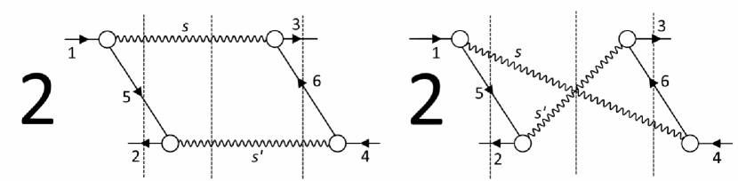
Figure 9: Two-phonon induced interaction $(F^{2phonon}_{ind})_{1234\_1}$, Eq.(32) and $(F^{2phonon}_{ind})_{1234\_2}$ Eq.(34), which are present in line 3 of Eq.(29),Fig.(8). Illustration of GSCs for two-phonon graphs in line 3 of Fig.(8). The cross-cuts show various 1p1h$\otimes$phonon and two-phonon configurations.

Here one can see a considerable difference from the two-phonon version of (Q)TBA ts2007 ; litva-ring-ts . Our method of introduction of two-phonon configurations shown in Eq.(28), Fig.7, gives much more complicated $\omega$-dependence for our two-phonon induced interactions $F^{2phonon}_{ind}$, Eq.(32) and Eq.(34), which correspond to the $\omega$-dependent two- quasiparticle amplitude $\Phi(\omega)$ in ts2007 ; litva-ring-ts . The difference is due to the use of a special factorization procedure for $\Phi(\omega)$ in ts2007 ; litva-ring-ts . Namely, it consists in inclusion of the correlations in the ph-pair entering the 1p1h$\otimes$phonon configuration, i.e., replacement of the uncorrelated pair with the phonon ts2007 . We think that our method with the full 1p1h-interaction amplitude $\Gamma$ shown in Eq.(28), Fig.7, is rather natural.

It is necessary to take into account the general specific features of the self-consistent approach. We mean the subtraction method developed in detail by V. Tselyaev tssubtraction ; litva-ring-ts . For the non-self-consistent approach, the analogous procedure was described and realized in kaev83 and ktZPhys , respectively, within the so-called refinement procedure that included the refined single-particle basis. As known, the energy density functional is constructed in the way to give the exact (in the limiting case) description of the nuclear ground state properties. Therefore, to avoid double counting of static contributions of complex configurations, which are already contained in the energy density functional, in our case it is necessary to subtract the static part $F^{2phonon}_{ind}(\omega=0)$ from $F^{2phonon}_{ind}(\omega)$. The detailed discussion of these rather numerous problems goes beyond the scope of our work.

The terms $\tilde{V}^{3}_{2phonon}$ in line 3 of Eq.(29), Fig.8, can be written through our two-phonon induced interactions, Eq.(32) and Eq.(34):

$$(\tilde{V}^{3}_{2phon})_{12\_1}(\varepsilon_{1},\omega)=$$

$$\sum_{34}\int(F^{2phonon}_{ind})_{1234\_1}(\varepsilon_{1},\varepsilon_{3})G_{3}(\varepsilon_{3}+\omega)G_{4}(\varepsilon_{3})\tilde{V}_{34}d\varepsilon_{3}$$

$$(\tilde{V}^{3}_{2phon})_{12\_2}(\varepsilon_{1},\omega)=$$

$$\sum_{34}\int(F^{2phonon}_{ind})_{1234\_2}(\varepsilon_{1},\varepsilon_{4})G_{3}(\varepsilon_{4}+\omega)G_{4}(\varepsilon_{4})\tilde{V}_{34}d\varepsilon_{4}$$ (37)

The final expressions for $(\tilde{V}^{3}_{2phon})_{12}(\varepsilon_{1},\omega)$ are rather cumbersome. They will be obtained and discussed in details somewhere else.

VI Energies and probabilities of transitions

Formulas for the energies and probabilities of transitions between the ground and excited states were obtained in [I] by means of direct and rather formal generalization of the respective formulas in TFFS Migdal ; Migdal2 . For the simplest case, which corresponds to the terms of $\tilde{V}^{1}$, Eq.(30) or lines 1 of Fig.8 and Fig.6, they were realized numerically without the TBA prescription in articles ktZPhys ; kt1984 for fine structure characteristics of isovector M1 resonances in magic nuclei. With the use of the TBA prescription and within the strongly improved TBA version, they were realized for the M1 resonance in ${}^{208}Pb$ recently in articles Tsel2019 ; Tsel2020 (see modifications of the TBA model there). In all these calculations there were no full explanation of the fine structure of the M1 resonance in ${}^{208}Pb$.

In [I] and in the present article, the next important step is realized, namely, due to inclusion of the first term of Eq.(10), Fig.3, the new phonon-induced interactions appear and, therefore, the $\varepsilon_{1}$-dependence of $\tilde{V}(\varepsilon_{1})$ is obtained for the first time.

This dependence, although interesting as it is, must be integrated and, therefore, is not seen in the strength function

$$S(\omega,\Delta)=\frac{dB(EL)}{d\omega}=-\frac{1}{\pi}Im\sum_{12}e_{q}V^{0}_{12}\rho_{21}(\omega+\imath\Delta),$$ (38)

where the density matrix $\rho=\overline{A}\tilde{V}$, $\overline{A}$ is a new generalized propagator and $\Delta$ is a smearing parameter that simulates a finite experimental resolution.

In our case, the equation for the density matrix $\rho$ is obtained by means of generalization of the equation for $\rho$ in [I]. From Eq.(38), one can obtain the transition probabilities and energy-weighed sum rule summed over an energy interval. This prescription is similar to the method of strength functions always used in the QPM method. As far as the important fine structure problem is concerned, the fine structure characteristics can be obtained at small numbers $\Delta$ = 10 keV or 1 keV. In Lyutor2018 such calculations for the PDR in ${}^{208}Pb$ were performed within the self-consistent TBA with the use of Skyrme forces, and they showed that it was impossible to obtain a reasonable agreement with the observable PDR fine structure. One can hope that the calculations within our approach should improve the situation.

VII Conclusion

In this article, the self-consistent TFFS has been consistently generalized for the case of accounting for PC effects in the energy region of PDR and GMR with the aim to take into account both 1p1h$\otimes$phonon and two-phonon configurations.

If to neglect the terms with $\delta F$, which probably give small contributions, our new results are contained in two variants of the newest equation for vertex $\tilde{V}$ shown in Fig.6 and Fig.8. The first variant, Section IV.A, Fig.6, contains 1p1h$\otimes$phonon configurations and the full amplitude 1p1h-interaction $\Gamma$, Eq.(3). This variant has some promising prospects for further development.

In the second variant, Section IV.B, Fig.8, the first step for further development has been realized within our TFFS generalization for the vertex $\tilde{V}$. Namely, through expansion of the full amplitude interaction $\Gamma$ in the RPA phonons, Eq.(27), it was possible to add two-phonon configurations to 1p1h$\otimes$phonon ones in line 3 (and also in lines 6,7,8 of Eq.(29), Fig.8, containing terms with $\delta F$) and to obtain the new two-phonon-induced interaction $F^{2phonon}_{ind}$.

In this second variant, both 1p1h$\otimes$phonon and two-phonon configurations, whose necessity was discussed in the Introduction, have been obtained. This allowed us to compare our results with the known QPM and QTBA approaches (in their variants for magic nuclei). We obtained a considerable complication as compared to them and article [1], not to mention the terms with $\delta F$. Our two-phonon part strongly differs from the TBA two-phonon part: it contains a more complex $\omega$-dependence, i.e. both two-phonon configurations with the numerators $[\omega\pm(\omega_{s^{\prime}}+\omega_{s})]^{-1}$ and 1p1h$\otimes$phonon configurations together, see Eq.(36).

In both variants we confirmed the previous model kaev83 shown in Fig.1 and, in fact, the standard TBA model ts89 but only as a particular case corresponding to line 1 in both variants shown in Fig.6 and Fig.8 (of course, provided that in the terms of line 1 and in other lines, the MCDD, or TBA prescription, will be applied, if necessary). Like in the considered case of [I], in both variants, the dynamic term with $\tilde{V}^{tad}$ is present. In the PDR+GMR energy region , this is a quite new effect and it is necessary to solve Eq.(7) for the two phonon creation amplitude $g_{11}$, in order to consider it. It can be done in the representation of single particle wave functions, but nobody has done it yet.

The two-phonon-induced interactions $F^{2phonon}_{ind}$ are caused by the phonon exchange in various channels (ph, hp, pp, hh). Their dependence on energy variables may be of interest both for nuclei and, probably, for other Fermi-systems and should be studied in future.

All the obtained formulas contain numerous GSCs in both 1p1h$\otimes$phonon and two-phonon configurations. These effects were investigated mainly within the GF formalism, however, it was not sufficient. They should be important, at least, in the problem of the PDR and GMR resonance fine structure, see recent article nester2020 and references in it.

Thus, in the present article, an important step to the direction of consistent inclusion of PC effects to the self-consistent TFFS has been made. In the nearest future we will finalize the general formulation of this approach in the PDR and GMR energy region with the aim to account for complex 1p1h$\otimes$phonon and two-phonon configurations. But at the present stage one can already see that the situation is rather complicated. Suffice it to compare the old approach shown in Fig.1 and the new one in Fig.8. We hope that several aspects of the particle-vibration coupling scheme have been clarified. Numerous future calculations must clarify the role of new considered effects. A further development is probably possible if to go beyond the main initial TFFS equations mentioned in Section II.A.

VIII ACKNOWLEDGMENTS

We are grateful to V.A. Khodel, and V.I. Tselayev for useful discussions. S.K. thanks Dr. A.C. Larsen and the Oslo group for stimulating cooperation in the PDR field. The reported study was funded by RFBR, project no.19-31-90186 and supported by the Russian Science Foundation, project no.16-12-10155.

References

- (1) D. Savran , T. Aumann, A. Zilges, Progr. Part. Nucl. Phys. 70, 210 (2013).
- (2) N. Paar, D. Vretenar, E. Khan, G. Colo, Rep. Prog. Phys. 70, 691 (2007).
- (3) A. Bracco, E.G. Lanza, and A. Tamii, Prog. Part. Nucl.Phys. 106, 360 (2019).
- (4) S.P. Kamerdzhiev, O.I. Achakovskiy, S.V. Tolokonnikov, M.I. Shitov, Phys. At. Nucl. 82, 366 (2019).
- (5) S. Kamerdzhiev, J. Speth, G. Tertychny, Phys. Rep. 393, 1 (2004).
- (6) A. Tamii, I. Poltoratska, P. von Neumann-Cosel, Y. Fujita, T. Adachi, C. A. Bertulani, J. Carter, M. Dozono, H. Fujita, K. Fujita, K. Hatanaka, D. Ishikawa, M. Itoh, T. Kawabata, Y. Kalmykov, A. M. Krumbholz, E. Litvinova, H. Matsubara, K. Nakanishi, R. Neveling, H. Okamura, H. J. Ong, B. Özel-Tashenov, V. Yu. Ponomarev, A. Richter, B. Rubio, H. Sakaguchi, Y. Sakemi, Y. Sasamoto, Y. Shimbara, Y. Shimizu, F. D. Smit, T. Suzuki, Y. Tameshige, J. Wambach, R. Yamada, M. Yosoi, and J. Zenihiro, Phys. Rev. Let. 107, 062502 (2011).
- (7) A. C. Larsen, J. E. Midtbø, M. Guttormsen, T. Renstrøm, S. N. Liddick, A. Spyrou, S. Karampagia, B. A. Brown, O. Achakovskiy, S. Kamerdzhiev, D. L. Bleuel, A. Couture, L. Crespo Campo, B. P. Crider, A. C. Dombos, R. Lewis, S. Mosby, F. Naqvi, G. Perdikakis, C. J. Prokop, S. J. Quinn, and S. Siem, Phys. Rev. C 97, 054329 (2018).
- (8) A. Repko, V.O. Nesterenko, J. Kvasil, and P.-G. Reinhard, Eur. Phys. J.A 55, 242 (2019).
- (9) N. Ryezayeva, T. Hartmann, Y. Kalmykov, H. Lenske, P. von Neumann-Cosel, V.Yu. Ponomarev, A. Richter, A. Shevchenko, S. Volz, and J.Wambach, Phys. Rev. Let. 89, 272502 (2002).
- (10) N. A. Lyutorovich, V. I. Tselyaev, O. I. Achakovskiy, and S. P. Kamerdzhiev, JETP Lett. 107, 659 (2018) .
- (11) A. B.Migdal, Theory of Finite Fermi Systems and Applications to Atomic Nuclei (Nauka, Moscow, 1965; Intersci., New York, 1967).
- (12) V. A. Khodel and E. E. Saperstein, Phys. Rep. 92, 183 (1982).
- (13) A. B.Migdal, Theory of Finite Fermi Systems and Applications to Atomic Nuclei, 2-ed Edition (Nauka, Moscow, 1983).
- (14) E. E. Saperstein and S. V. Tolokonnikov, Phys. At.Nucl. 79, 1030 (2016).
- (15) D.Voitenkov, S. Kamerdzhiev, S. Krewald, E.E. Saperstein, S.V. Tolokonnikov, Phys. Rev. C 85, 054319 (2012).
- (16) S.P. Kamerdzhiev, Sov. J. Nucl. Phys. 38, 188 (1983).
- (17) V. I. Tselyaev, Sov. J. Nucl. Phys. 50, 780 (1989).
- (18) V. Tselyaev, Phys. Rev. C 75, 024306 (2007).
- (19) A. Avdeenkov, S. Goriely, S. Kamerdzhiev, S. Krewald, Phys. Rev. C 83, 064316 (2011).
- (20) S. P. Kamerdzhiev and V.N. Tkachev, Z. Phys. A334, 19 (1989).
- (21) S. P. Kamerdzhiev and V.N. Tkachev, Phys. Lett. 142B, 225 (1984).
- (22) P.F. Bortignon, R.A. Broglia, Nucl. Phys. A 371, 405 (1981).
- (23) P.F. Bortignon, R.A. Broglia,G.F. Bertsch, J.Pacheco, Nucl. Phys. A 460, 149 (1986).
- (24) S.P. Kamerdzhiev, A.V. Avdeenkov, O.I. Achakovskiy, Phys. Atom. Nucl. 77, 1303 (2014).
- (25) V. Tselayev, N. Lyutorovich, J. Speth, P.-G.Reinhard, Phys. Rev. C 97, 044308 (2018).
- (26) E.Litvinova and P.Schuck, Phys. Rev. C 100, 064320 (2019).
- (27) S.P. Kamerdzhiev, M. I. Shitov, Eur.Phys.J.A 80, 265 (2020).
- (28) V.G. Soloviev, Theory of atomic nuclei: quasi-particles and phonons (Institute of physics, Bristol and Philadelphia, USA, 1992).
- (29) F. Knapp, N. Lo Iudice, P. Vesely, F. Andreozzi, G. De Gregorio, and A. Porrino, Phys. Rev. C 92, 054315 (2015).
- (30) V. A. Khodel, A.P. Platonov, E.E. Saperstein, J. Phys. G: Nucl. Phys. 6, 1199 (1980).
- (31) V. A. Khodel, Sov. J. Nucl. Phys. 24, 367 (1976).
- (32) E.Litvinova, P.Ring, V.Tselyaev, Phys.Rev. C 88, 044320 (2013).
- (33) V. Tselyaev, N. Lyutorovich, J. Speth, P.-G. Reinhard, and D. Smirnov, Phys. Rev. C 99, 064329 (2019).
- (34) V. Tselyaev, N. Lyutorovich, J. Speth, P.-G. Reinhard, Phys.Rev. C 102,064319 (2020).
- (35) V.I. Tselyaev, Phys.Rev. C 88, 054301 (2013).
- (36) L. M. Donaldson, J. Carter, P. von Neumann-Cosel, V. O. Nesterenko, R. Neveling, P.-G. Reinhard,I. T. Usman, P. Adsley, C. A. Bertulani, J. W. Brümmer, E. Z. Buthelezi, G. R. J. Cooper, R. W. Fearick,S. V. Förtsch, H. Fujita, Y. Fujita, M. Jingo, N. Y. Kheswa, W. Kleinig, C. O. Kureba, J. Kvasil, M. Latif, C. W. Li, J. P. Mira, F. Nemulodi, P. Papka, L. Pellegri, N. Pietralla, V. Yu. Ponomarev, B. Rebeiro, A. Richter, N. Yu. Shirikova, E. Sideras-Haddad, A. V. Sushkov, F. D. Smit G. F. Steyn, J. A. Swartz, and A. Tamii, Phys. Rev. C 102, 064327 (2020).