Temperature Controlled Open Quantum System Dynamics using Time-dependent Variational Method

Abstract

Dirac-Frenkel variational method with Davydov $\text{D}_{2}$ trial wavefunction is extended by introducing a thermalization algorithm and applied to simulate dynamics of a general open quantum system. The algorithm allows to control temperature variations of a harmonic finite size bath, when in contact with the quantum system. Thermalization of the bath vibrational modes is realised via stochastic scatterings, implemented as a discrete-time Bernoulli process with Poisson statistics. It controls bath temperature by steering vibrational modes’ evolution towards their canonical thermal equilibrium. Numerical analysis of the exciton relaxation dynamics in a small molecular cluster reveals that thermalization additionally provides significant calculation speed up due to reduced number of vibrational modes needed to obtain the convergence.

I Introduction

Obtaining dynamics of open quantum systems, i.e., quantum systems that are identified as separate from its environment, yet remain in thermal contact with it, is one of the most general quantum mechanical problems. Its applicability range from excited state relaxation in optical response (Dorfman et al., 2016; Mukamel, 1995), energy transport in molecular aggregates (Jakučionis et al., 2018; Chorošajev et al., 2017; Schröter et al., 2015; Chorošajev et al., 2014; Valkunas et al., 2013; May and Kühn, 2011), photosynthetic complexes (Jang and Mennucci, 2018; Thyrhaug et al., 2018; Malý et al., 2016; Chenu and Scholes, 2015) and others (Sjakste et al., 2018; Flesch et al., 2008; Lombardo and Turiaci, 2013; Yu and Zhang, 2008; Ruostekoski and Walls, 1998). Prevalent theoretical description is given in terms of system- bath model in constant temperature bath conditions (Breuer and Petruccione, 2007; Weiss, 2012), where the system degrees of freedom are coupled to the bath-induced thermal fluctuations representing the environment, e.g., phonons or vibrational motion of surrounding molecules. Fluctuations are modeled by an infinite number of quantum harmonic oscillators constituting the quantum bath at thermal equilibrium.

These conditions can be fulfilled using the reduced density matrix approach (Valkunas et al., 2013; Mukamel, 1995). First perturbation order, with respect to the system-bath coupling, leads to the reduced equations of motion of the system-only variables, while the bath is averaged out. Then the system variables indirectly depend on the bath degrees of freedom via fluctuation correlation functions, which are well-behaved analytical functions. At the second perturbation order (Breuer and Petruccione, 2007; Valkunas et al., 2013), equations of motion are reminiscent of the Pauli master equation with relaxation coefficients calculated with respect to the thermal equilibrium. However, now the resulting equations can lead to unphysical results, e.g., negative probabilities (Montoya-Castillo et al., 2015). The more complicated fourth order equations of motion include divergent parameters and are often avoided (Jang et al., 2002). Non-perturbative, numerically exact approach of hierarchical equations of motion for the exponential fluctuation correlation functions is available to obtain exact dynamics (Tanimura, 1990, 2006; Xu and Yan, 2007), chain-mapping techniques together with the time-dependent density matrix renormalization group are alternatively possible for structured environments (Tamascelli et al., 2019; Prior et al., 2010). However, computational costs limit these methods to models with just few degrees of freedom. A well known method of stochastic Schrödinger equation requires averaging over many entangled trajectories to obtain dynamics at finite temperature (Abramavicius and Abramavicius, 2014; Appel and Di Ventra, 2009; Biele and D’Agosta, 2012; Diósi and Strunz, 1997; de Vega et al., 2005; Link and Strunz, 2017). Its hierarchical realisation (Hartmann and Strunz, 2017) improves convergence, meanwhile, thermofield dynamics approach tries to directly compute thermally averaged dynamics by mapping the initial thermal density matrix onto a fictitious bath vacuum state and then coupling system to it (Reddy and Prasad, 2015; Ritschel et al., 2015; Borrelli and Gelin, 2016; Chen and Zhao, 2017). Alternativelly, dissipative dynamics can be obtained by straightforward addition of a linear friction coefficient to the model Hamiltonian (Martinazzo et al., 2006), however, it only applies at zero temperature. Yet, in all these cases, thermal state of the nearest surrounding is not under control.

An important aspect of the bath, more explicitly, of the finite number of bath oscillators, is its heat capacity. For a single quantum harmonic oscillator the heat capacity in the limit of weak system-bath coupling is given by

$$c\left(\beta^{-1}\right)= (\beta\omega)^{2}\frac{\exp(\beta\omega)}{(\exp(\beta\omega)-1)^{2}}\ ,$$ (1)

here throughout the paper $\hbar=1$, $\beta=\left(k_{\text{B}}T\right)^{-1}$ is an inverse temperature, $\omega$ is the oscillator frequency. When the system exchanges energy with a bath made of such oscillators, its temperature may be affected. If the system-bath energy exchange is excessively large, the thermal energy can accumulate in the bath oscillators and this will effectively change thermostat temperature (Abramavicius et al., 2018). In most cases, the bath heating effect is undesirable as, in the system-bath models, the bath is generally supposed to represent a constant temperature thermostat.

On the other hand, the bath heating effect could be related to the natural phenomenon of molecular local heating (Chen and Sorbello, 1993; Ichikawa et al., 2007), i.e., if a molecule quickly dissipates a large amount of thermal energy to its environment, e.g., due to exciton-exciton annihilation (Gulbinas et al., 1996; Valkunas and Gulbinas, 1997; Gulbinas et al., 2006) or ultrafast molecular internal-conversion (Balevičius et al., 2018; Balevičius Jr et al., 2019), the local heating of the molecule nearest surrounding takes place and the further cooling process, the quantum thermalization (Choi et al., 2019; Scarani et al., 2002), becomes an important ingredient to consider when describing the corresponding experiments.

In this work, we introduce the thermalization algorithm to the time dependent variational theory that allows explicit control over the bath temperature. By varying the bath size and the thermalization rate, both the degree of bath heating and the cooling time can be adjusted. These properties allow to mimic realistic physical conditions, making presented approach superior to the density operator based approaches, where the bath heating is excluded, and to the explicit bath models, where the bath temperature is not controlled.

II Fluctuating exciton model

We consider a molecular aggregate made of $N$ coupled chromophores at specific sites. In the simplest case, the sites represent distinct molecules that can be electronically excited by, e.g., laser or sunlight irradiation in visible spectral region. Vibrational normal modes of molecules and of the surrounding medium will be treated as the baths of harmonic oscillators. Each chromophore is directly affected only by its own intramolecular vibrations and of its closest environment, therefore, a separate and uncorrelated (local) manifold of vibrational modes $q=1,2,\ldots,Q$ is associated with each chromophore. Such model is characterized by a Hamiltonian $\hat{H}=\hat{H}_{\text{S}}+\hat{H}_{\text{B}}+\hat{H}_{\text{SB}}$, with system, bath and system-bath coupling terms being

$$\hat{H}_{\text{S}}= \sum_{n}\varepsilon_{n}\hat{a}_{n}^{\dagger}\hat{a}_{n}+\sum_{n,m}^{n\neq m}J_{nm}\hat{a}_{n}^{\dagger}\hat{a}_{m}\ ,$$ (2)

$$\hat{H}_{\text{B}}= \sum_{n,q}\omega_{nq}\hat{b}_{nq}^{\dagger}\hat{b}_{nq}\ ,$$ (3)

$$\hat{H}_{\text{SB}}= -\sum_{n}\hat{a}_{n}^{\dagger}\hat{a}_{n}\sum_{q}\omega_{nq}g_{nq}\left(\hat{b}_{nq}^{\dagger}+\hat{b}_{nq}\right)\ ,$$ (4)

Here $\varepsilon_{n}$ denotes $n$th chromophore electronic excitation energy $J_{nm}$ is the resonant coupling between $n$th and $m$th chromophores, while $\hat{a}_{n}^{\dagger}$ and $\hat{a}_{n}$ are the corresponding electronic excitation creation and annihilation bosonic operators. Frequency of the $q$th vibrational mode in the $n$th bath is $\omega_{nq}$, the electron-vibrational coupling is characterized by $g_{nq}$, while $\hat{b}_{nq}^{\dagger}$ and $\hat{b}_{nq}$ are the creation and annihilation bosonic operators of the $q$th mode in the $n$th bath.

In the following we consider only single electronic excitation in the aggregate. Time evolution of a non-equilibrium state is described by Davydov $\text{D}_{2}$ wavefunction (Frenkel and Frenkel, 1936; Sun et al., 2010)

$$|\Psi_{\text{D}_{2}}\rangle=\sum_{n}^{N}\alpha_{n}\left(t\right)\hat{a}_{n}^{\dagger}\hat{a}_{n}|0\rangle_{\text{el}}\times\prod_{m,q}^{N,Q}|\lambda_{mq}\left(t\right)\rangle\ ,$$ (5)

where $\alpha_{n}\left(t\right)$ is the electronic excitation amplitude, $|0\rangle_{\text{el}}=\prod_{n}|0\rangle_{n}$ is the global ground state, when all sites are in their electronic ground states. $|\lambda_{mq}\left(t\right)\rangle$ is the coherent state of the $q$th mode in the $m$th bath (Zhang et al., 1990; Kais and Levine, 1990). It is fully described by the time-dependent complex displacements, $\lambda_{mq}\left(t\right)$. The time dependent Dirac-Frenkel variational method allows to obtain equations of motion for parameters $\alpha_{n}$, $\lambda_{mq}$ (Chorošajev et al., 2014; Jakučionis et al., 2018; Chen et al., 2018; Yan et al., 2020)

$$\frac{\text{d}\alpha_{n}\left(t\right)}{\text{dt}}=-\text{i}\alpha_{n}\left(t\right)\varepsilon_{n}-\text{i}\sum_{m}^{m\neq n}\alpha_{m}\left(t\right)J_{nm}$$

$$\qquad+\text{i}\alpha_{n}\left(t\right)\sum_{q}\omega_{nq}\left(2g_{nq}-h_{q}\right)\text{Re}\left(\lambda_{nq}\left(t\right)\right)\ ,$$ (6)

$$\frac{\text{d}\lambda_{mq}\left(t\right)}{\text{dt}}=-\text{i}\omega_{mq}\left(\lambda_{mq}\left(t\right)-h_{q}\left(t\right)\right)\ .$$ (7)

Here $h_{q}\left(t\right)=\sum_{i}^{N}g_{iq}\left|\alpha_{i}\left(t\right)\right|^{2}$ is the site population-weighted electron-vibrational coupling strength. First line in Eq. (6) describes dynamics of an isolated system. Accordingly, the first term on the right hand side of Eq. (7) describes isolated oscillators. Other terms are due to the system-bath interaction.

Description of the model at the given temperature $T$ requires creation of statistical ensemble. This is achieved by Monte Carlo sampling over a statistical thermal ensemble, i. e., over initial bath oscillator displacements $\lambda_{mq}\left(0\right)$, sampled from the Glauber-Sudarshan probability distribution (Glauber, 1963)

$$\mathcal{P}\left(\lambda_{mq}\right)=\mathcal{Z}^{-1}\exp\left(-\left|\lambda_{mq}\right|^{2}\left[\text{e}^{\beta\omega_{mq}}-1\right]\right)\ .$$ (8)

The ensemble describes canonical statistics of quantum harmonic oscillators, which applies to our model prior to external perturbations. The ensemble averaged quantities will be denoted by $\left\langle\cdots\right\rangle_{\text{th}}$. The ensemble of exciton trajectories allows to describe irreversible excitation energy relaxation. While the initial thermal state before excitation can be properly defined, the bath accepts energy during exciton relaxation and the state of the bath after relaxation is away from equilibrium. Equations of motion guarantee energy conservation, hence the combined system-bath cannot thermalize. In order to thermalize the bath, we extend the original model by introducing the secondary bath (we will refer to the local baths as the primary baths). Effective heat capacity of the secondary bath is infinite, hence, the bath can be characterized by a constant temperature, $T_{\infty}$. The secondary bath will not be treated explicitly: modes of the primary baths interact with the secondary bath via stochastic scattering events, or quantum jumps (Plenio and Knight, 1998; Luoma et al., 2020), which affect the kinetic energy of primary baths modes.

The scattering statistics follows Poisson distribution $P_{mq}\left(\theta,\tau\right)=\frac{1}{\theta!}\left(\tau\nu_{mq}\right)^{\theta}\text{e}^{-\tau\nu_{mq}}$, which defines the probability of observing $\theta$ scattering events per time interval $\tau$ with individual event scattering rate $\nu_{mq}$. Poisson statistics is obtained by simulating a discrete-time Bernoulli process (Kampen, 2007; Bertsekas and Tsitsiklis, 2008) in a limit of $\tau\rightarrow 0$ and $\nu_{mq}\tau\ll 1$. This is realized in simulations by dividing the total evolution time $t_{\text{total}}$ into equidistant length $\tau$ intervals. At the end of each interval, for each mode in the primary bath, we flip a biased coin with probability $\nu_{mq}\tau$ of landing “heads”. If the coin lands heads, we shift momentum of the mode $p_{mq}\left(kt\right)=\sqrt{2}\text{Im}\lambda_{mq}\left(kt\right)$ to a value drawn from the Glauber-Sudarshan distribution, see Eq. (8), while the coordinate remains unchanged. Otherwise, if coin lands tails, no changes are done. To obtain converged statistics, we apply the thermalization algorithm to every trajectory of the thermal ensemble.

III Simulation results

We first demonstrate control of the primary bath temperature of the simplest possible system, a single, $N=1$, chromophore unit. For demonstration we set up artificial conditions: the initial primary bath temperature $T_{1}\left(0\right)=300\ \text{K}$, the secondary bath is at $T_{\infty}=200\ \text{K}$. The primary bath consists of $Q=750$ vibrational modes with frequencies, $\omega_{q}=\omega_{0}+\left(q-1\right)\Delta\omega$. An offset by $\omega_{0}=0.01\ \text{cm}^{-1}$ is introduced for stability and a step size $\Delta\omega=1\ \text{cm}^{-1}$. The coupling parameters $g_{nq}$ follow the super-Ohmic spectral density function $C^{"}\left(\omega\right)=\omega^{s}\exp\left(-\omega/\omega_{c}\right)$ with $s=2$, $\omega_{\text{c}}=100\ \text{cm}^{-1}$ (Kell et al., 2013; Jakučionis et al., 2018). The number of modes and discretization parameters are sufficient to obtain convergent model dynamics. For thermalization, we consider scattering rates of all modes to be equal $\nu_{mq}\rightarrow\nu$, and the scattering step size $\tau=0.01\ \text{ps}^{-1}$. Thermal ensemble consists of $5000$ trajectories.

Figure 1: Phase space trajectory of one specific bath mode $\omega_{q}=100\ \text{cm}^{-1}$ for a single excited chromophore calculated with various scattering rates $\nu$. Initial temperature of the primary bath is $T_{1}\left(0\right)=300\ \text{K}$ and the secondary bath is at a constant temperature $T_{\infty}=200\ \text{K}$. Scattering step size is $\tau=0.01\ \text{ps}$. Wiggles in dynamics are due to finite size ensemble averaging (5000 trajectories).

In Fig. (1) the coordinate $\left\langle x_{1q}\right\rangle_{\text{th}}=\left\langle\sqrt{2}\text{Re}\lambda_{1q}\right\rangle_{\text{th}}$ and momentum $\left\langle p_{1q}\right\rangle_{\text{th}}=\left\langle\sqrt{2}\text{Im}\lambda_{mq}\right\rangle_{\text{th}}$ phase space trajectory of a single $100\ \text{cm}^{-1}$ frequency vibrational mode, calculated with various scattering rates $\nu$ is presented. The oscillator, in the absence of thermalization, evolves along a closed trajectory around $x_{1q}^{\text{min}}=\sqrt{2}g_{1q}$. Applying thermalization procedure, a dissipative type trajectory is observed. The coordinate $\left\langle x_{1q}\right\rangle_{\text{th}}$ equilibrates to $x_{1q}^{\text{min}}$ (equilibrium is shifted from zero due to coupling with the system), while momentum $\left\langle p_{1q}\right\rangle_{\text{th}}$ approaches zero. The thermalization time can be adjusted by changing the scattering rate, $\nu$. Both weakly damped and overdamped regimes become available.

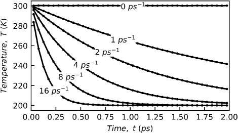
Figure 2: The primary bath temperature $T_{1}\left(t\right)$ calculated with various scattering rates $\nu$. Initial temperature of the primary bath is $T_{1}\left(0\right)=300\ \text{K}$ and the secondary bath is at a constant temperature $T_{\infty}=200\ \text{K}$. Scattering step size is $\tau=0.01\ \text{ps}$.

Transient temperature of the primary bath can be estimated (Abramavicius et al., 2018) by computing the average kinetic energy $\left\langle K_{mq}\left(t,\epsilon\right)\right\rangle_{\text{th}}$ over time interval $\epsilon$. The parameter $\epsilon$ then implies the resolution. For the whole primary bath the transient temperature is then given by

$$T_{m}\left(t\right)=\frac{1}{k_{\text{B}}Q}\sum_{q=1}^{Q}\omega_{mq}\ln\left(1+\frac{\omega_{mq}}{2\left\langle K_{mq}\left(t,\epsilon\right)\right\rangle_{\text{th}}}\right)^{-1}\ .$$ (9)

In Fig. (2) we present the primary bath temperature calculated with $\epsilon=50\ \text{fs}$ and various scattering rates, $\nu$. In the absence of thermalization, the primary bath temperature remains at the initial value of $T_{1}\left(0\right)=300\ \text{K}$. Meanwhile, thermalization introduces cooling of the primary bath down to the temperature of the secondary bath. The scattering rate, $\nu$, allows to control the thermalization time.

The temperature control and stability considerably affects the electronic excitation dynamics. To demonstrate the sensitivity of the excitation evolution to the thermalization we consider a linear $N=3$ chromophore aggregate, with chromophore transition energies $0,\ 250,\ 500\ \text{cm}^{-1}$, and nearest neighbor coupling $J=100\ \text{cm}^{-1}$. Excited states of such chromophore aggregate are excitons (Valkunas et al., 2013; van Amerongen et al., 2000). They represent electronic excitations delocalized over several sites with time dependent delocalization length (Chorošajev et al., 2016). Hence, we switch to the eigenstate basis (exciton representation, defined by $\hat{H}_{\text{S}}\psi^{(\mathrm{exc})}=\varepsilon\psi^{(\mathrm{exc})}$): $\rho_{e}^{\text{(exc)}}\left(t\right)=\sum_{n,m}\left(\psi_{ne}^{(\mathrm{exc})}\right)^{\star}\left\langle\alpha_{n}^{\ast}\left(t\right)\alpha_{m}\left(t\right)\right\rangle_{th}\psi_{me}^{(\mathrm{exc})}$. The initial electronic state correspond to the optically excited highest energy exciton eigen state. The parameters of the primary baths of chromophores are the same as above, however, now the initial primary bath temperature and the secondary bath temperature is the same $T_{m}\left(0\right)=T_{\infty}=77\ \text{K}$. The thermal ensemble consists of $240$ trajectories. In Fig. (3) we present exciton state populations $\rho_{e}^{\text{exc}}\left(t\right)$ and the primary bath temperatures $T_{m}\left(t\right)$ calculated in (i) the dense primary bath discretization regime without thermalization (the bath discretization step size is $\Delta\omega=1\ \text{cm}^{-1}$, $Q=750$ vibrational modes per site), in (ii) the sparse discretization regime without thermalization ($\Delta\omega=50\ \text{cm}^{-1}$, $Q=15$) and (iii) the sparce discretized bath with thermalization ($\nu=2.5\ \text{ps}^{-1}$).

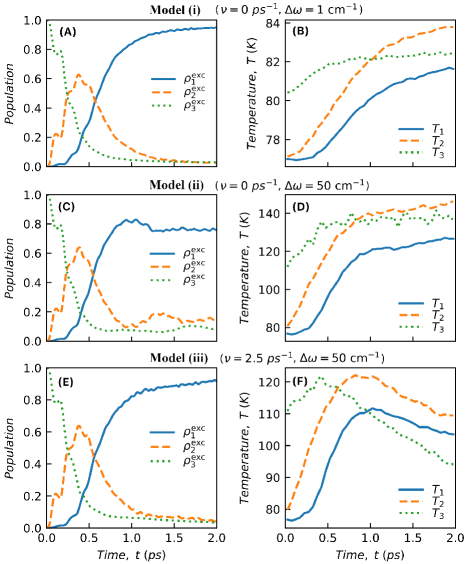
Figure 3: Multi site-bath model exciton state populations $\rho_{n}^{\text{exc}}\left(t\right)$ and local bath temperatures $T_{m}\left(t\right)$ calculated in (i) the dense primary bath discretization regime without thermalization, (ii) the sparse discretization regime without thermalization and (iii) the sparcely discretized bath with thermalization ($\nu=2.5\ \text{ps}^{-1}$).

Consider the excitation dynamics without thermalization. In models (i) and (ii) exciton populations sequentially relax to lower energy exciton states, eventually reaching the lowest energy state. (Moix et al., 2012; Subasi et al., 2012; Gelzinis and Valkunas, 2020). The final population distribution in the sparse regime, model (ii), significantly differs from the dense case. Origin of the discrepancy is two-fold: the bath recursion time $t_{\text{rec}}=2\pi/\Delta\omega$ for model (ii) is shorter than the calculation time $t_{\text{rec}}<t_{\text{total}}$, and the sparse primary bath shows significant growth of the bath temperature, compare Fig. (3B and 3D). Both of these drawbacks are addressed by introducing the bath thermalization in model (iii). Looking at Fig. (3E), we see that the exciton population dynamics and steady state values for model (iii) become quantitatively comparable to case of model (i).

IV Discussion

A single quantum harmonic oscillator is characterized by a specific heat $c(\beta^{-1})<k_{\text{B}}$, which depends on temperature as given by Eq. (1). For a given set of bath oscillators the specific heat at a given temperature can be estimated, however, the harmonic oscillators of the bath as defined by Eq. (3) do not exchange energy. Accordingly, as the system relaxes, only a few in-resonant oscillators accept the energy and diverges away from equilibrium (Chin et al., 2013). Hence, the temperature at which excitation dynamics occur no longer match the initial bath temperature - local heating takes place.

A straightforward approach to avoid heating is to increase the bath density of states until dynamics of interest converges (in our model, this is achieved by increasing the number of bath oscillators). However, this is acceptable only for small systems, since computation effort scales quadratically with both number of sites and bath oscillators. Thermalization can be utilized to steer the bath to the required temperature. Additional merit of thermalization is the significant reduction of the the number of vibrational modes needed per bath. Our simulations show convergence with just $15$ modes per bath while maintaining comparable exciton relaxation dynamics (Fig. 3).

In effort to reduce the computational effort, Wang et al. have used (Wang et al., 2016) a logarithmic bath discretization. However, high frequency representation of the continuous spectral density becomes poor. Our model is in line with explicit surrogate Hamiltonian (Baer and Kosloff, 1997) and its stochastic realization (Katz et al., 2008; Torrontegui and Kosloff, 2016; Habecker et al., 2019), while our approach does not require the explicit modeling of the secondary bath, it still maintaining proper quantum dynamics in the system.

The time-dependent variational approach with Davydov $\text{D}_{2}$ ansatz can be improved by considering more complex Davydov ans$\ddot{a}$tze family members, e.g., multitude of $\text{D}_{1}$ ansatz (multi-$\text{D}_{1}$) and multi-$\text{D}_{2}$ (Zhou et al., 2015; Wang et al., 2016; Zhou et al., 2016; Chen et al., 2018) or its Born-Oppenheimer approximated variant (Jakučionis et al., 2020), $\text{sD}_{2}$. In either way, they all suffer from finite bath heating capacity, in most cases, even stronger than the $\text{D}_{2}$ ansatz, because of significantly increased computational effort needed to propagate numerous bath oscillators. Work is in progress on adapting the presented thermalization algorithm to these more intricate ans$\ddot{a}$tze.

In conclusion, we present a system-bath model with stochastic bath thermalization using the time-dependent variational approach with Davydov $\text{D}_{2}$ ansatz. Thermalization allows to steer bath vibrational modes evolution towards equilibrium thermal state of selected temperature in a controlled way, and at the same time, for the bath to still maintain an aspect of being coupled to the system. In addition, by analysing exciton relaxation dynamics of a chromophore aggregate with thermalization, we found the exciton dynamics to converge with much smaller number of bath modes, significantly speeding up numerical computation.