D’ya like DAGs? A Survey on Structure Learning and Causal Discovery

Abstract.

Causal reasoning is a crucial part of science and human intelligence. In order to discover causal relationships from data, we need structure discovery methods. We provide a review of background theory and a survey of methods for structure discovery. We primarily focus on modern methods which leverage continuous optimization, and provide reference to further resources such as benchmark datasets and software packages. Finally, we discuss the assumptive leap required to take us from structure to causality.

1. Introduction

Causal understanding has been described as ‘part of the bedrock of intelligence’ (Li et al., 2020b), and is one of the fundamental goals of science (Glymour et al., 2019; Pearl, 2009; van der Laan and Rose, 2011; Bareinboim et al., 2020; van der Laan and Starmans, 2014; van der Laan and Rose, 2018). It is important for a broad range of applications, including policy making (Kreif and DiazOrdaz, 2019), medical imaging (Castro et al., 2019), advertisement (Bottou et al., 2013), the development of medical treatments (Petersen et al., 2017), the evaluation of evidence within legal frameworks (Pearl, 2009; Siegerink et al., 2016), social science (Vowels, 2020; Hernan, 2018; Grosz et al., 2020), biology (Triantafillou et al., 2017), and many others. It is also a burgeoning topic in machine learning and artificial intelligence (Xu et al., 2020; Scholkopf, 2019; Li et al., 2020a; Bengio, 2019; Goyal and Bengio, 2020; Vowels et al., 2020a; Garcez and Lamb, 2020), where it has been argued that a consideration for causality is crucial for reasoning about the world. In order to discover causal relations, and thereby gain causal understanding, one may perform interventions and manipulations as part of a randomized experiment. These experiments may not only allow researchers or agents to identify causal relationships, but also to estimate the magnitude of these relationships.

Unfortunately, in many cases, it may not be possible to undertake such experiments due to prohibitive cost, ethical concerns, or impracticality. For example, to understand the impact of smoking, it would be necessary to force different individuals to smoke or not-smoke. Researchers are therefore often left with non-experimental, observational data. In the absence of intervention and manipulation, observational data leave researchers facing a number of challenges: Firstly, observational datasets may not contain all relevant variables - there may exist unobserved/hidden/latent factors (this is sometimes referred to as the third variable problem). Secondly, observational data may exhibit selection bias - for example, younger patients may in general prefer to opt for surgery, whereas older patients may prefer medication. Thirdly, the causal relationships underlying these data may not be known a priori - for example, are genetic factors independent causes of a particular outcome, or do they mediate or moderate an outcome? These three challenges affect the discovery and estimation of causal relationships.

To address these challenges, researchers in the fields of statistics and machine learning have developed numerous methods for uncovering causal relations (causal discovery) and estimating the magnitude of these effects (causal inference) from observational data, or from a mixture of observational and experimental data. Under various (often strong) assumptions, these methods are able to take advantage of the relative abundance of observational data in order to infer causal structure and causal effects. Indeed, observational data may, in spite of the three challenges listed above, provide improved statistical power and generalizability compared with experimental data (Deaton and Cartwright, 2018).

In this paper we review relevant background theory and provide a survey of methods which perform structure discovery (sometimes called causal induction (Griffiths and Tenenbaum, 2009)) with observational data or with a mixture of observational and experimental data. A number of reviews, surveys and guides are already available (see e.g. (Heinze-Deml et al., 2018; Glymour et al., 2019; Spirtes and Zhang, 2016)), however, these reviews cover combinatoric approaches to causal discovery, whereas we primarily focus on the recent flurry of developments in continuous optimization approaches. Furthermore, the existing reviews are relatively short, and we attempt to provide a more scoping introduction to the necessary background material. We also seek to provide more extensive coverage of continuous optimization approaches than other current reviews, which focus on combinatoric approaches. Finally, we provide references to further useful resources including datasets and openly available software packages.

The structure of this survey is as follows: Following an overview of relevant background information in Section 2, we provide an overview of approaches to structure discovery in Section 3, including a list of common evaluation metrics. In Section 4 we briefly outline a range of combinatoric approaches, before focusing on continuous optimization approaches in Section 5. We begin 6 by referencing several additional resources including reviews, guides, datasets, and software packages. We also provide a summary and discussion of the methods covered in Section 6, and note various opportunities for future work and future direction. Many of the methods we review in this survey seek to discover and interpret the learned structure causally. Whilst this is a laudable aim, we are reminded of important commentaries (e.g.,(Humphreys and Freedman, 1996; Freedman and Humphreys, 1999; Dawid, 2008)) which argue for appropriate skepticism and care when making the leap from observation to causality via causal discovery methods. We therefore conclude Section 6, as well as this survey as a whole, by providing a discussion on these issues.

2. Background - Definitions and Assumptions

In this section we provide working definitions of key concepts in structure discovery. We include a presentation of a common framework used in structure discovery (namely, that of structured graphical representations) as well as a number of common assumptions.

2.1. Causality and SCMs

In spite of some notable reluctance to treat graphs learned from observational data as causal (Dawid, 2008; Humphreys and Freedman, 1996; Freedman and Humphreys, 1999), we acknowledge that it is a common and worthwhile aim, and begin by presenting a working definition of causality and its popular systematization in Structural Causal Models (SCMs). Causality eludes straightforward definition (Spirtes et al., 2000), and is often characterized intuitively with examples involving fires and houses (Pearl, 2009), firing squads (Hopkins and Pearl, 2003), and bottles and rocks (Hopkins and Pearl, 2005). One definition of what is known as counterfactual causality is given by by Lewis (1973) (Lewis, 1973) as follows:

”We think of a cause as something that makes a difference, and the difference it makes must be a difference from what would have happened without it. Had it been absent, its effects – some of them, at least, and usually all – would have been absent as well”.

Lewis’ definition is counterfactual in the sense that he effectively describes ‘what would have happened if the cause had been A*, given that the effect was B when the cause was A’. Seemingly, this definition is compatible with the Pearlian school of causal reasoning. Specifically, in the context of what are known as SCMs:

”Given two disjoint sets of variables $X$ and $Y$, the causal effect of $X$ on $Y$, denoted as… $P(y|do(x))$, is a function from $X$ to the space of probability distributions on $Y$. For each realization of $x$ of $X$, $P(y|do(x))$ gives the probability of $Y=y$ induced by deleting from the model [$x_{i}=f_{i}(pa_{i},u_{i}),i=1...,n,$] all equations corresponding to variables in $X$ and substituting $X=x$ in the remaining equations.”

This definition (Pearl, 2009, p.70) requires further examination. Firstly, the model $x_{i}=f_{i}(pa_{i},u_{i}),i=1...,n,$ is a Structural Equation/Causal Model (SEM/SCM) which indicates assignment of the value $x_{i}$ in the space of $X$ to a function of its structural parents $pa_{i}$ and exogenous noise $u_{i}$. We elaborate on what parents are (as well as children, descendants etc.) below. Secondly, the $do$ notation (Pearl, 2009) indicates intervention, where the value of $x$ is set to a specific quantity. The structure (including attributes such as parents) can be represented graphically using various types of graphical models (e.g., Directed Acyclic Graphs). Figure 1 shows the relationship between a DAG and a general Structural Equation Model. Sometimes this SEM is also called a Functional Causal Model (FCM), where the functions are assumed to represent the causal mechanisms (Goudet et al., 2018). The use of the assignment operator ‘$:=$’ makes explicit the asymmetric nature of these equations. In other words, they are not to be rearranged to solve for their inputs. To transform these relationships from mathematical relationships to causal relations, the Causal Markov Condition is imposed, which simply assumes that arrows (and their entailed conditional independencies) represent causal dependencies (Peters et al., 2017, p.105-6).

The ultimate benefit of the graphical and structural model frameworks is that they, at least in principle and under some strong assumptions, enable us to use observational data to answer scientific questions such as ‘how?’, ‘why?’, and ‘what if?’ (Pearl and Mackenzie, 2018).

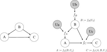
Figure 1. Transitioning from a typical DAG representation (left) to a structural equation model (right). Grey vertices are unobserved/latent random variables.

2.2. Graphical Models

For background on graphical models, see work by Koller and Friedman (2009) (Koller and Friedman, 2009). We follow a similar formalism to Peters et al. (2017) (Peters et al., 2017) and Strobl (2018) (Strobl, 2018). A graph $\mathcal{G}(\mathbf{X},\mathcal{E})$ represents a joint distribution $P_{\mathbf{X}}$ as a factorization of $d$ variables $\mathbf{X}=\{X_{1},...,X_{d}\}$ using $d$ corresponding nodes/vertices $v\in\mathbf{V}$ and connecting edges $(i,j)\in\mathcal{E}$, where $(i,j)$ indicates an edge between $v_{i}$ and $v_{j}$. If two vertices $i$ and $j$ are connected by an edge we call them adjacent, and, can also denote this in terms of the corresponding variables $\mathbf{X}$ as $X_{i}\rightarrow X_{j}$ or $X_{i}\leftarrow X_{j}$ (directed), $X_{i}$ — $X_{j}$ (undirected), $X_{i}\leftrightarrow X_{j}$ (bidirected), $X_{i}\kern 3.0pt\hbox{-}\kern-1.0pt\hbox{-}\kern-1.0pt\hbox{-}\kern-1.0pt\hbox{$\circ$}\kern 3.0ptX_{j}$ or $X_{i}\kern 3.0pt\hbox{$\circ$}\kern-1.0pt\hbox{-}\kern-1.0pt\kern-1.0pt\hbox{-}\kern-1.0pt\hbox{-}\kern-1.0pt\hbox{-}\kern 3.0ptX_{j}$ (partially undirected), $X_{i}\kern 3.0pt\hbox{$\circ$}\kern-2.0pt\hbox{$\rightarrow$}\kern 3.0ptX_{j}$ or $X_{i}\kern 3.0pt\hbox{$\leftarrow$}\kern-2.0pt\hbox{$\circ$}\kern 3.0ptX_{j}$ (partially directed), or $X_{i}\kern 3.0pt\hbox{$\circ$}\kern-1.0pt\hbox{-}\kern-1.0pt\hbox{-}\kern-1.0pt\hbox{$\circ$}\kern 3.0ptX_{j}$ (nondirected). A graph comprising entirely undirected edges forms a skeleton. It is also possible to have self-loops, although these occur relatively infrequently in the structure discovery literature. These different edge types allow us to define a range of graph types and relationships.

An undirected path exists if there are edges connecting two vertices regardless of the edge types between them. In contrast, a directed path constitutes directed edges with consistent arrowhead directions. We can define a parent $pa_{j}$ as a vertex $v_{i}$ with child $v_{j}$ connected by a directed edge $X_{i}\rightarrow X_{j}$ such that $(i,j)\in\mathcal{E}$ but $(j,i)\notin\mathcal{E}$. Further upstream parents are ancestors of downstream descendants if there exists a directed path constituting $i_{k}\rightarrow j_{k+1}$ for all $k$ in a sequence of vertices. An immorality or v-structure describes when two non-adjacent vertices are parents of a common child. A collider is a vertex where incoming directed arrows converge.

It is possible for directed cycles to occur when following a directed path results in the visitation of a vertex more than once (e.g., $X_{i}\rightarrow X_{j}\rightarrow X_{k}\rightarrow X_{i}$). Many phenomena in nature exhibit cyclic properties and feedback, and ignoring this possibility has the potential to induce bias (Strobl, 2018; Sacks et al., 2005; Ghassami et al., 2020). If all edges are directed, and there are no cycles, we have the well-known class of Directed Acyclic Graphs (DAGs). On the other hand, if all edges are directed but there is no restriction preventing cycles, we have a Directed Graph (DG).

2.3. The Markov Assumption, $d$-Separation, and $d$-Faithfulness

The graphs are usually assumed to fulfil the Markov property, such that the implied joint distribution factorizes according to the following recursive decomposition, characteristic of Bayesian networks (Pearl, 2009):

(1) $$P(\mathbf{X})=\prod_{i}^{d}P(X_{i}|pa_{i})$$

This decomposition relates to the notion of $d$-separation. Two vertices $X_{i}$ and $X_{k}$ are $d$-separated by the set of vertices $\mathbf{S}$ if $X_{j}\in\mathbf{S}$ in any of the following structural scenarios (Peters et al., 2017):

(2) $$\begin{split}X_{i}\rightarrow X_{j}\rightarrow X_{k}\\ X_{i}\leftarrow X_{j}\leftarrow X_{k}\\ X_{i}\leftarrow X_{j}\rightarrow X_{k}\\ \end{split}$$

They are also $d$-separated if $X_{j}$ and none of the descendants of $X_{j}$ are in set $\mathbf{S}$ in the following structural scenario (collider):

(3) $$\begin{split}X_{i}\rightarrow X_{j}\leftarrow X_{k}\\ \end{split}$$

If the DAG’s $d$-separation properties hold (an assumpion of faithfulness - see below), they imply Markovian conditional independencies in the joint distribution, which can be denoted as $X_{i}\rotatebox[origin={c}]{90.0}{$\models$}_{P_{\mathbf{X}}}X_{k}|X_{j}$. In terms of the DAG, disjoint (i.e., non-overlapping) sets of variables $\mathbf{A}$ and $\mathbf{B}$ are $d$-separated by disjoint set of variables $\mathbf{S}$ in graph $\mathcal{G}$ if $\mathbf{A}\rotatebox[origin={c}]{90.0}{$\models$}_{d-sep}\mathbf{B}|\mathbf{S}$ (Peters et al., 2017), and are, conversely $d$-connected if this conditional independence in the graph does not hold.

The assumption of $d$-faithfulness is that any conditional independencies implied by the graph, according to its $d$-separation properties, are reflected in the joint distribution $P_{\mathbf{X}}$. More formally (Peters et al., 2017, p.107), for joint distribution $P_{\mathbf{X}}$ and DAG $\mathcal{G}$, the assumption of $d$-faithfulness holds if $\mathbf{A}\rotatebox[origin={c}]{90.0}{$\models$}_{P_{\mathbf{X}}}\mathbf{B}|\mathbf{C}\implies\mathbf{A}\rotatebox[origin={c}]{90.0}{$\models$}_{d-sep}\mathbf{B}|\mathbf{C}$. One example of a violation of $d$-faithfulness occurs when the influence of two paths cancel each other out, resulting in a DAG with different implied conditional independencies to those present in the joint distribution.

2.4. Markov Equivalence Class (MEC) and Completed Partially Directed Acyclic Graphs (CPDAGs)

The conditional independence constraints implied by a graph’s $d$-separation properties are not always enough to uniquely identify it. Whether a graph can be uniquely identified is known as the problem of identifiability, and a significant body of work has been devoted to identifying scenarios for which the true graph is identifiable (e.g., linear functional form with non-Gaussian errors (Hoyer et al., 2008b), or nonlinear functional forms with additive noise (Hoyer et al., 2008a)). As such, there are situations in which multiple graphs satisfy the same conditional independencies. For example, conditional independence implied by $X_{i}\rotatebox[origin={c}]{90.0}{$\models$}X_{k}|X_{j}$ is present in the graph $X_{i}\rightarrow X_{j}\rightarrow X_{k}$ as well as the graphs $X_{i}\leftarrow X_{j}\leftarrow X_{k}$ and $X_{i}\leftarrow X_{j}\rightarrow X_{k}$, in spite of the fact that these graphs have drastically different causal implications. The class of graphs which represent the same set of conditional independencies together constitute the Markov Equivalence Class (MEC). Graphs belong to the same equivalence class when they have the same skeleton and the same immoralities (Verma and Pearl, 1991).

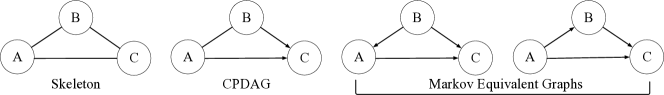
Figure 2. Showing a skeleton, a CPDAG, and the Markov Equivalence set of graphs. Variable C is a collider, and so the direction of incoming arrows can be identified from conditional independencies.

Completed Partially Directed Acyclic Graphs (CPDAGs) can be used to represent an MEC. In CPDAGs, an edge is only directed if there is only one graph in the MEC with an edge in that direction, otherwise, if there is uncertainty about the direction, it is left ‘non-directed’ using $\circ$--$\circ$. One might wonder whether there are any MECs without undirected edges, and indeed there are. A collider or v-structure forms an MEC with only one valid DAG: $X_{i}\rightarrow X_{j}\leftarrow X_{k}$. This is because conditioning on $X_{j}$ makes $X_{i}$ and $X_{k}$ $d$-connected. An example of a skeleton graph, a CPDAG, and corresponding MEC graphs are shown in Figure 2.

2.5. Assumption: Sufficiency

One of the challenges with using observational data is the assumption that all relevant data have been collected/observed. This is less problematic in the case of Randomized Controlled Trials (RCTs) because the randomization itself helps mitigate the effect of confounding which would otherwise imbalance the treatment and control groups. In observational settings, unobserved confounding can significantly bias effect estimates (even reversing their direction). Whilst it is possible to try to infer hidden confounders from observational data using latent variable models (see e.g. (Wang and Blei, 2019; Louizos et al., 2017; Vowels et al., 2020a), a large number of causal discovery methods assume sufficiency, which is the assumption that there are no unobserved confounders. The assumption of sufficiency is strong and may often be inappropriate or overly restrictive. If the assumption does not hold, the set of observed variables is (causally) insufficient (Bhattacharya et al., 2020) and a DAG comprising only the observed variables can not be used (and the DAG is said to not be closed under marginalization) (Hu and Evans, 2020).

2.6. Acyclic Directed Mixed Graphs (AGMGs) and Maximal Ancestral Graphs (MAGs) and $m$-separation

In the presence of unobserved confounding, an Acyclic Directed Mixed Graph (ADMG) may be used. ADMGs represent hidden confounding as bidirected edges. For example, the confounding relationship given by $X_{i}\leftarrow H\rightarrow X_{j}\rightarrow X_{k}$ can, in the absence of $H$, be represented in an ADMG as $X_{i}\leftrightarrow X_{j}\rightarrow X_{k}$.

Maximal Ancestral Graph (MAG) can also be used to represent hidden confounding, and have the further capacity of representing selection bias (i.e. as might occur when a certain sub-population is sampled). MAGs satisfy the following three properties (Richardson and Spirtes, 2002, 2003; Ali et al., 2009): (1) there are no directed cycles (acyclicity); (2) if an edge $X_{i}\leftrightarrow X_{j}$ exists (which implies $X_{i}$ is the spouse of $X_{j}$) then there are no directed paths between $X_{i}$ and $X_{j}$; (3) if an edge $X_{i}$ — $X_{j}$ exists (which implies $X_{i}$ is the neighbour $X_{j}$) then $X_{i}$ and $X_{j}$ have no spouses or parents. This edge is used to represent selection bias (i.e. where a subpopulation has been sampled according to some condition).

The definitions of ancestor and descendent translate naturally from DAGs (see above) to MAGs, as does the definition for $d$-separation, which becomes $m$-separation. In the latter case, the conditions for $d$-separation in Equations 2 and 3 hold, substituting any confounding variable relationships (e.g., $X_{i}\leftarrow H\rightarrow X_{j}$) with a bidirected arrow (e.g., $X_{i}\leftrightarrow X_{j}$). In the presence of selection bias, a $X_{i}$ — $X_{j}$ edge can be used. Readers are directed to (Richardson and Spirtes, 2002, 2003; Ali et al., 2009) for a more detailed and formal exposition.

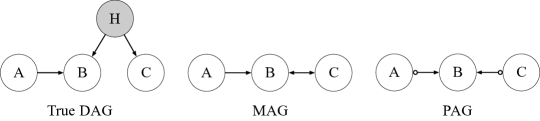
Figure 3. Showing the relationship between the true DAG and its representation using a MAG and a PAG. Shaded vertex is a hidden/unobserved confounding variable. Adapted from (Peters et al., 2017, p.179).

The assumption of $m$-faithfulness translates naturally from $d$-faithfulness for DAGs (see above) to MAGs, according to the conditional independencies implied by $m$-separation.

2.7. Partial Ancestral Graphs (PAGs)

Similarly to how the MEC of a set of DAGs was represented using a CPDAG, the MEC for a set of MAGs can be representing using a Partially Ancestral Graph (PAG). PAGs make use of edges $X_{i}\kern 3.0pt\hbox{$\circ$}\kern-1.0pt\hbox{-}\kern-1.0pt\hbox{-}\kern-1.0pt\hbox{$\circ$}\kern 3.0ptX_{j}$, $X_{i}\kern 3.0pt\hbox{$\circ$}\kern-2.0pt\hbox{$\rightarrow$}\kern 3.0ptX_{j}$, and $X_{i}\kern 3.0pt\hbox{-}\kern-1.0pt\hbox{-}\kern-1.0pt\hbox{-}\kern-1.0pt\hbox{$\circ$}\kern 3.0ptX_{j}$. Edges with arrowheads indicate that arrowheads are present in all MAGs in the associated MEC. A tail (i.e., an edge without either a circle mark or an arrowhead) indicates that the tail is present in all MAGs in the associated MEC. Circle marks (as with CPDAGs) indicate uncertainty in the edge mark, such that the MEC contains MAGs in which the edge mark is either a tail or an arrowhead. (Heinze-Deml et al., 2018; Peters et al., 2017). An example of a DAG and its equivalent MAG and PAG are shown in Figure 3.

2.8. Other Definitions and Assumptions

Other types of graph used to represent causal structure include Partially Oriented Induced Path Graphs (POIPGs) (Spirtes et al., 2000; Peters et al., 2017), Single World Intervention Graphs (SWIGs) (Breskin et al., 2018; Richardson and Robins, 2013a, b), $\sigma$-connection graphs (Forré and Mooij, 2018), undirected graphs (Battaglia et al., 2018), interaction and component graphs for dynamic systems (Cummins et al., 2019), Maximal Almost Ancestral Graphs (MAAGs) (Strobl, 2018), psi-ECs (Jaber et al., 2020), Patterns (Zhang et al., 2020a), and arid, bow-free, and ancestral ADMGs (Bhattacharya et al., 2020). There are also other types of assumptions relating to the functional form of the structural relationships (e.g., linear or non-linear) as well as the parametric form of the marginals and the errors (e.g., Gaussian or non-Gaussian). In the interests of brevity, we have not discussed these additional graph-types and assumptions here, but encourage interested readers to consult the listed references.

3. Structure Discovery Methods

We consider four approaches to structure discovery: constraint-based, score-based, those exploiting structural asymmetries, and those exploiting various forms of intervention. We begin by introducing these four approaches. Each structure discovery method may be sub-categorized into those which seek to identify a graphical structure via combinatoric/search-based approaches, or those which seek to identify a graphical structure via continuous optimization. Previous reviews exist for the former (e.g., (Heinze-Deml et al., 2018; Glymour et al., 2019; Spirtes and Zhang, 2016)), so we primarily focus on the latter. Finally, methods may be categorized as local, whereby edges are tested one at a time, or global, whereby an entire graph candidate is tested.

3.1. Constraint-Based and Score-Based Approaches

Most constraint-based approaches test for conditional independencies in the empirical joint distribution in order to construct a graph that reflects these conditional independencies. According to the discussion above, there are often multiple graphs that fulfil a given set of conditional independencies, and so it is common for constraint-based approaches to output a graph representing some MEC (e.g., a PAG). Unfortunately, conditional independence tests require large sample sizes to be reliable, and Shah and Peters (2020) (Shah and Peters, 2020) discuss further challenges to controlling Type I errors.

Score-based approaches test the validity of a candidate graph $\mathcal{G}$ according to some scoring function $S$. The goal is therefore stated as (Peters et al., 2017):

(4) $$\hat{\mathcal{G}}=\mbox{argmax}_{\mathcal{G}\mbox{ over }\mathbf{X}}S(\mathcal{D},\mathcal{G})$$

where $\mathcal{D}$ represents the empirical data for variables $\mathbf{X}$. Common scoring functions include the Bayesian Information Criterion (BIC) (Geiger and Heckerman, 1994), the Minimum Description Length (as an approximation of Kolmogorov Complexity) (Janzing and Schölkopf, 2010; Grünwald and Vitányi, 2008; Kalainathan et al., 2020), the Bayesian Gaussian equivalent (BGe) score (Geiger and Heckerman, 1994), the Bayesian Dirichlet equivalence (BDe) score (Heckerman et al., 1995), the Bayesian Dirichlet equivalence uniform (BDeu) score (Heckerman et al., 1995), and others (Imoto et al., 2002; Hyvärinen and Smith, 2013; Huang et al., 2018).

3.2. Exploiting Structural Asymmetries

There is no way to rule out scenarios whereby a joint distribution admits SCMs indicating either of the structural directions $X_{i}\rightarrow X_{j}$ or $X_{i}\leftarrow X_{j}$, thereby making the induction of causal directionality from observation alone, impossible. However, if some additional assumptions are made about the functional and/or parametric forms of the underlying true data-generating structure, then one can exploit asymmetries in order to identify the direction of a structural relationship. These asymmetries manifest in various ways, including non-independent errors, measures of complexity, and dependencies between marginals and cumulative distribution functions. Methods which exploit such asymmetries are typically local methods, as they are only able to test edges one at a time (pairwise/bivariate causal directionality), or to test triples (with the third variable being an unobserved confounder) (Hoyer et al., 2008b). They may, of course, be extended to construct full-graphs by iteratively testing pairwise relationships (see e.g. the Information-Geometric Causal Inference algorithm (Janzing et al., 2012)). We now briefly provide some examples of structural asymmetries, and direct interested readers to Mooij et al. (2016) (Mooij et al., 2016b) for a detailed review.

3.2.1. Additive Noise

Given the linear structural equations $X=U_{X}$ and $Y=X+U_{Y}$ such that $U_{Y}\rotatebox[origin={c}]{90.0}{$\models$}X$, we expect the residuals from a regression on the data from this generative model to reflect the $U_{Y}\rotatebox[origin={c}]{90.0}{$\models$}X$ property. Interestingly, if at most $X$ or $U_{Y}$ is non-Gaussian, then the causal direction (i.e. $X\rightarrow Y$) is identifiable (Peters et al., 2017; Hyvärinen et al., 2001; Kagan et al., 1973; Glymour et al., 2019). This is illustrated in Figure 4. The true structural relationship $X=U_{X}$ and $Y=X+U_{Y}$ is used to generate data, where $U_{X}$ and $U_{Y}$ are non-Gaussian (they are uniformly distributed). In plot A, $Y$ is regressed onto $X$ (aligning with the true structural directionality), and it can be seen from plot B that the residuals following this regression are uncorrelated with $X$. Conversely, and as shown in plot C, when $X$ is regressed onto $Y$(conflicting with the true structural directionality), it can be seen in plot D that this results in dependence between the residuals and $Y$.

The example given in Figure 4 depicts the non-Gaussian, linear case. Unfortunately, the assumption that (a) the data generating process is linear and (b) that the noise are sufficiently non-Gaussian to facilitate reliable identifiability may be overly restrictive in practice. The post-non-linear additive noise model assumes that the data are generated according to the structural equations $X=U_{X}$ and $Y=f(X)+U_{Y}$ where $f$ is sufficiently non-linear, and does not assume that either $U_{Y}$ or $X$ are non-Gaussian. Similarly to the linear non-Gaussian case above, the post-non-linear additive noise model exhibits structural asymmetries that are reflected in the (in)dependence of regression residuals (Peters et al., 2017; Glymour et al., 2019; Hoyer et al., 2008a).

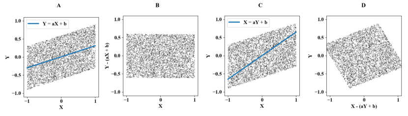
Figure 4. The true structural relationship is $Y=X+U_{Y}$ and $X=U_{X}$ where $U_{X}$ and $U_{Y}$ are uniform noise sources. (A) shows the regression line when regressing $Y$ onto $X$, and (B) shows the corresponding residuals plotted against $X$. (C) shows the regression line when regressing $X$ onto $Y$ and (D) shows the corresponding residuals plotted against $Y$. Together, these demonstrate that under the assumption of linear functional form and non-Gaussian noise, the true structural direction is identifiable as the one for which $X$ is independent of the residuals, as indicated in (B). Example adapted from (Peters et al., 2017).

3.2.2. Information Geometric Properties

From a causal perspective, the information geometric approach to identifying structural directionality takes inspiration from the concept of independent mechanisms. Assuming that the true structural direction is $X\rightarrow Y$, the concept of independent mechanisms holds that $P(X)$ contains no information about $P(Y|X)$, and vice versa. A common illustrative example (Peters et al., 2017) involves measurements of temperature $Y$ at weather stations of different altitudes $X$. Regardless of the distribution of weather station altitudes $P(X)$, the mechanisms linking altitude to temperature (e.g. the law determining the relationship between the temperature and pressure of a gas) exist independently, and changing the temperature around a weather station does not increase its altitude.

Numerically, this scenario may be easily demonstrated by considering the inverse transform sampling method for transforming a uniform distribution $P(X)$ into a target distribution $P(Y)$ using the inverse cumulative distribution function. The uniform distribution is clearly independent of the function being used to transform it, but this independence does not hold for the transformed distribution. More generally, if $Y=f(X)$, the independence of mechanisms implies with high likelihood that $P_{X}$ will be independent of the mechanism $f$. The corollary is that there exists dependence between $P_{Y}$ and $f^{-1}$ (Janzing et al., 2012). Assuming a structural direction $X\rightarrow Y$ via function $f$, the inverse function $f^{-1}$ satisfies $\mbox{cov}[\log f^{-1},p_{Y}]\geq 0$ (Janzing et al., 2012, 2015; Peters et al., 2017).

It is worth noting various limitations to this approach, particularly with respect to its application to causal discovery in real-world systems. Firstly, it assumes that the mechanism $f$ is deterministic. Secondly, it assumes that $f$ is sufficiently non-linear that it may be used to identify dependence. Thirdly, real-world systems may (in addition to having non-deterministic mechanisms) demonstrate adaptation between cause and effect, such that $P_{X}$ is no longer independent of $f$.

Figure 5. Showing the differences between a hard/structural intervention (middle) and a soft/parametric intervention (right) on the original DAG (left). It can been that the parametric intervention preserves structural relationships. Adapted from (Eberhardt and Scheine, 2006, p.986).

Figure 6. Starting with the CPDAG on the left, where the structural direction between vertices A and B is unknown, intervening on B allows us to orient this edge. In the middle, the edge from A to B is removed following intervention on B (this is illustrated with the slash). On the right, an intervention on B does not remove the edge from B to A, and the effect of the intervention flows to A.

3.3. Interventions and Adjustment Sets

If interventional data are available, we are able to reduce the number of graphs in our MEC. An intervention can be denoted using Pearl’s do operator (Pearl, 2009) such that, ”for each realization of $x$ of $X$, $P(y|do(x))$ gives the probability of $Y=y$ induced by deleting from the model [$x_{i}=f_{i}(pa_{i},u_{i}),i=1...,n,$] all equations corresponding to variables in $X$ and substituting $X=x$ in the remaining equations.” Such interventions can be hard/perfect/structural/atomic/deterministic, or soft/imperfect/parametric, depending on whether a variable is set to a specific value, or whether the variable and its relationship to its neighbours is modified in some way (e.g., by changing the noise distribution $u$). Graphically, a hard intervention can be represented by removing all incoming arrows (from parents) to a vertex, and setting that vertex to the value $x$ (Peters et al., 2017, p.88-91). For a structural equation model $X=U_{X}$, $Y=f(X)+U_{Y}$ and $Z=g(X)+h(Y)+U_{Z}$, an intervention $Y=4$ would entail $X=U_{X}$ (unmodified), $Y=4$ (modified), and $Z=g(X)+h(4)+U_{Z}$ (modified). Thus it can be seen that only $Y$ and its descendants have been affected by the intervention, leaving $X$ unchanged. In contrast to hard interventions, a parametric intervention preserves the structure of the intervention itself, introducing an additional vertex and affecting the conditional distribution of the intervened variable. Parametric interventions also preserve any correlations deriving from unobserved/hidden confounders (Eberhardt and Scheine, 2006). This difference is illustrated in Figure 5.

In order to demonstrate how interventions can be used to narrow the equivalence set (and in some cases make the true graph identifiable), consider the graphs in Figure 6. Starting with the CPDAG on the left, where the edge from A to C is undirected because the direction of the edge cannot be ascertained from conditional independencies alone. Intervening (hard) on B allows us to orient this edge by comparing the resulting distribution under intervention. If the edge is oriented $A\rightarrow B$ then the intervention has the effect of ‘removing’ this edge. Conversely, if the edge is oriented $B\rightarrow A$ then the intervention does nothing to remove this arrow, and the downstream variable $A$ should change accordingly.

Another way to view interventions from the perspective of independencies is to consider their formulation in terms of adjustment sets. Following (Peters and Bühlmann, 2015; Cinelli et al., 2020; Pearl, 2009): $p(y|do(X=x))=p(y)$ if $Y$ is a parent of $X$ (i.e., $Y\in pa_{X}$). In words, intervening on $X$ does not change $y$ because $X$ is ‘downstream’ of $Y$. Secondly, if $Y\not\in pa_{X}$, then:

(5) $$p(y|do(X=x))=\sum_{pa_{X}}p(y|x,pa_{X})p(pa_{X})$$

Here, the marginalized interventional distribution $p(y|do(X=x))$ is being computed using the adjustment set (in this case $pa_{X}$ is a valid adjustment set). More generally, the interventional distribution can be calculated as:

(6) $$p(y|do(X=x))=\sum_{\mathbf{z}}p(y|x,\mathbf{z})p(\mathbf{z})$$

when $\mathbf{z}$ is a valid adjustment set for this particular interventional distribution. Note that sets including mediators and descendants of mediators (where $B$ in the graph $A\rightarrow B\rightarrow C$ is a mediator) are not valid adjustment sets for finding $C|do(A)$. See Cinelli et al. (2020) (Cinelli et al., 2020) for a ”Crash course in good and bad controls”.

For a detailed review of different types of interventions and their implications, readers are directed to Eberhardt & Scheines (2006) (Eberhardt and Scheine, 2006). Suffice to say there are many ways to leverage different types of intervention, including multiple interventions on different vertices, or single interventions applied to multiple nodes. Finally, there is work investigating the use of data representing unknown or uncertain interventions, whereby it is not known which variables have been intervened on (Ke et al., 2020a; Rothenhausler et al., 2015; Eaton and Murphy, 2007; Mooij et al., 2016a). The use of intervention also yields what is known as an Interventional Equivalence Class (IEC), representing the set of graphs compatible with a given intervention(s).

3.4. Causality Over Time

Consider a graph $X\rightarrow Y$ for the case where $X$ and $Y$ vary over time. In this scenario, a single right-arrow is not sufficient to detail whether $X$ causes $Y$ on an intra-timepoint basis (i.e, contemporaneously), or on an inter-timepoint (i.e., lagged) basis. Indeed, at different points in time, and over different lags, the direction of causality may switch. In these cases it is common to unroll the graph over time, such that each instance of variables $X^{t}$ and $Y^{t}$ and their structural relationships over time are modelled explicitly.

There are then two types of causality considered in the context of time series. The most common (which is generally considered to be the industry standard, particularly in economics) is Granger causality (Granger, 1980). If a variable $X$ ‘Granger-causes’ $Y$, then it means that $Y^{t}\not\!\perp\!\!\!\perp X^{<t}|Y^{<t}$ (Peters et al., 2017, pp.207), where $<t$ indicates timepoints previous to $t$. If this is the case, then the predictability of $Y^{t}$ will decrease when $X^{<t}$ is removed from the model (because $X$ contains unique information for predicting $Y$), when accounting for previous values of $Y$.

The first thing to note about Granger causality is that it tends to fail in the presence of contemporaneous effects (Peters et al., 2017, pp.207), owing to difficulties with identifiability. The second, and perhaps more important aspect of Granger causality, is that it is only applicable if separability holds. Separability refers to the independence of the variables in the absence of causal interactions. Unfortunately, this is rarely the case in dynamic systems, where the current state of a variable may be heavily determined by the past of another (e.g., consider a predator-prey model, where both population levels are always functions of each other).

This failure of Granger causality was noted by Granger himself, and has motivated the development and application of dynamic-causality; in particular, methods deriving from Sugihara et al.‘s Convergent Cross Mapping methods (Sugihara et al., 2012; Ye et al., 2015). The methods operate using time delayed embeddings or shadow manifolds. These shadow manifolds are constructed by concatenating time-lagged versions of the original time series. This process has been shown according to Takens’ theorem (Tak, 1981), to be sufficient in recovering the dynamics of the full system even if only one, or a limited number, of observational variables are used. Dynamic or CCM-causality has shown great promise in applications to ecosystems and genetics (Sugihara et al., 2012; Ye et al., 2015). The general idea behind these methods is to exploit asymmetries that exist between the compactness of neighbourhoods of points in the shadow manifolds. If $X\rightarrow Y$ in a CCM-causal sense, then points which are tightly clustered in the ‘effect shadow manifold’ of $Y$ should also be tightly clustered in the ‘cause shadow manifold’ of $X$. This characteristic does not hold in the reverse direction (nor if there is no causal interaction in either direction), and this asymmetry enables us to identify causal interactions and directionality.

3.5. Evaluation Metrics

There are a number of common metrics used for evaluating the performance of causal discovery algorithms. The metrics given below are those used to evaluate the success of edge discovery. Other score metrics can be used to measure model fit (such as the log likelihood or the Bayesian Information Criterion). For a more detailed discussion on structural discovery metrics, readers are directed to work by de Jongh (2009) (de Jongh and Druzdzel, 2009).

True Positive Rate (TPR) (Heinze-Deml et al., 2018, p.383): Assuming the probability of an edge $p(a_{ij})$ can be thresholded by $t\in(0,1)$, TPR is defined as $\mbox{TPR}_{t}=|\{(i,j):p(a_{ij})\geq t\}\cap\mathbf{S}|/|\mathbf{S}|$ where $\mathbf{S}$ is the set of ground truth edges (i.e., $\{(i,j):a^{*}_{ij}=1\}$).

False Positive Rate (FPR) (Heinze-Deml et al., 2018, p.383): Assuming the probability of an edge $p(a_{ij})$ can be thresholded by $t\in(0,1)$, FPR is defined as $\mbox{FPR}_{t}=|\{(i,j):p(a_{ij})\geq t\}\cap\hat{\mathbf{S}}|/|\hat{\mathbf{S}}|$ where $\hat{\mathbf{S}}$ is the set of ground truth missing edges (i.e., $\{(i,j):a^{*}_{ij}=0\}$).

Area Over Curve (AOC) (Heinze-Deml et al., 2018, p.383): Simply $(1-\mbox{Area Under Curve (AUC)}$ for the AUC of $(FPR_{t},TPR_{t})$ where the threshold $t$ is varied between 0 and 1. Either the AUC or AOC can be used as a structure discovery performance metric.

Structural Hamming Distance (SHD): Is the number of required changes to the graph for it to match the ground truth. It is the sum of missing edges, extra edges, and incorrect edges (de Jongh and Druzdzel, 2009).

Structural Interventional Distance (SID) (Peters and Bühlmann, 2015): Is a count of the number of vertex pairs $(i,j)$ for which the intervention $p(x_{j}|do(X_{i}=x))$ would be incorrect if the estimated graph (as opposed to the ground-truth graph) were used for the associated adjustment set. It is therefore particularly well suited for causal inference tasks (Lachapelle et al., 2020, p.7).

4. Combinatoric/Search Based Approaches

The number of possible DAGs increases super-exponentially with the number of variables (Robinson, 1973). As noted by Peters et al. (2017) (Peters et al., 2017), the number of possible DAGs for 10 variables is $>4\times 10^{18}$. As such, the search problem is NP-hard (Chickering, 1996), and this will later motivate the use of continuous optimization approaches to graph learning.

Method	Year	Type	Suff.	Faith.	Acycl.	Interv.	Output
PC (Spirtes et al., 2000)	1993	constraint	yes	yes	yes	no	CPDAG
CCD (Richardson, 1996)	1996	constraint	yes	yes	both	no	PAG
FCI (Spirtes et al., 2000)	2000	constraint	no	yes	yes	no	PAG
TPDA (Cheng et al., 2002)	2002	constraint	yes	yes	yes	no	CPDAG
CPC (Ramsey et al., 2006)	2006	constraint	yes	relaxed	yes	no	CPDAG
KCL (Sun et al., 2007)	2007	constraint	yes	yes	yes	no	CPDAG
ION (Tillman et al., 2008)	2008	constraint	no	yes	yes	no	PAG
IDA (Maathuis et al., 2009)	2009	constraint	yes	yes	yes	yes	DAG
cSAT+ (Triantafillou et al., 2010)	2010	constraint	no	yes	yes	no	PCG
KCI-test (Zhang et al., 2012)	2012	constraint	yes	yes	yes	no	CPDAG
RFCI (Colombo et al., 2012)	2012	constraint	no	yes	yes	no	PAG
CHC (Gámez et al., 2012)	2012	constraint	yes	yes	yes	no	PDAG
SAT (Hyttinen et al., 2013)	2013	constraint	no	yes	no	yes	DG
Parallel-PC (Le et al., 2014)	2014	constraint	yes	yes	yes	no	CPDAG
RPC (Harris and Drton, 2013)	2013	constraint	yes	yes	yes	no	CPDAG
PC-stable (Colombo and Maathuis, 2014)	2014	constraint	both	yes	both	no	CPDAG
COmbINE (Triantafillou and Tsamardinos, 2015)	2015	constraint	no	yes	yes	yes	summary SMCMs
backshift (Rothenhausler et al., 2015)	2015	-	no	no	no	yes	DG
IGSP (Yang et al., 2018)	2018	constraint	yes	relaxed	yes	yes	I-MEC
$\sigma$-CG (Forré and Mooij, 2018)	2018	constraint	no	yes	no	yes	$\sigma$-connection graphs
CCI (Strobl, 2018)	2018	constraint	no	yes	no	no	MAAG
FCI-soft (Kocaoglu et al., 2019)	2019	constraint	no	relaxed	yes	yes	I-MEC
IBSSI (Chicharro et al., 2020)	2020	constraint	no	yes	yes	yes	DAG
CD-NOD (Huang et al., 2020)	2020	constraint	no	yes	both	yes	—–
psi-FCI (Jaber et al., 2020)	2020	constraint	no	relaxed	yes	yes	Psi-EC
LCDI (Zhang et al., 2020a)	2020	constraint	no	yes	yes	yes	Pattern
EG (Elidan and Gould, 2009)	2009	score	yes	yes	yes	no	BT-DAG
TWILP (Parviainen et al., 2014)	2014	score	yes	yes	yes	no	BT-DAG
K2 (Cooper and Herskovits, 1992)	1992	score	no	yes	yes	no	CPDAG
LB-MDL (Lam and Bacchus, 1994)	1994	score	yes	yes	yes	no	DAG
HGC (Heckerman et al., 1995)	1995	score	yes	yes	yes	no	CPDAG
GES (Chickering, 2002)	2002	score	yes	yes	yes	no	CPDAG
OS (Teyssier and Koller, 2005)	2005	score	yes	yes	yes	no	DAG
HGL (He et al., 2005)	2005	score	yes	yes	yes	yes	CPDAG
Meinshausen (Meinshausen and Bühlmann, 2006)	2006	score	yes	-	no	no	UG
Graphical Lasso (Friedman et al., 2008)	2008	score	yes	-	no	no	UG
BC (Banerjee et al., 2008)	2008	score	yes	-	no	no	UG
TC (Pellet and Elisseeff, 2008)	2008	score	yes	yes	yes	no	CPDAG
HG (He and Geng, 2008)	2008	score	yes	yes	yes	yes	DAG
Adaptive Lasso (Shojaie and Michailidis, 2010)	2010	score	yes	yes	yes	no	DAG
GIES (Hauser, 2012)	2012	score	yes	yes	yes	yes	PDAG
CD (Fu and Zhou, 2013)	2013	score	yes	yes	yes	yes	DAG
GBN learner (van de Geer and Bühlmann, 2013)	2013	score	yes	no	yes	no	CPDAG
GES-mod (Alonso-Barba et al., 2013)	2013	score	yes	yes	yes	no	CPDAG
Pen-PC (Ha et al., 2015)	2015	score	yes	yes	yes	no	CPDAG
Scalable GBN (Aragam and Zhou, 2015)	2015	score	yes	no	yes	no	DAG
K-A* (Scanagatta et al., 2016)	2016	score	yes	yes	yes	no	DAG
NS-DIST (Han et al., 2016)	2016	score	yes	no	yes	yes	DAG
MIP-GD (Park and Klabjan, 2017)	2017	score	yes	yes	yes	no	CPDAG
CD2 (Gu et al., 2018)	2018	score	yes	yes	yes	yes	DAG
SP (Raskutti and Uhler, 2018)	2018	score	yes	relaxed	yes	no	CPDAG
VAR (Young et al., 2018)	2018	score	yes	yes	both	no	DG
GSF (Huang et al., 2018)	2018	score	yes	yes	yes	no	CPDAG
bQCD (Tagasovska et al., 2020)	2020	score	yes	yes	yes	no	Bi
GCL (Varando, 2020)	2020	score	no	-	no	no	GCLM
GGIM (Fitch, 2020)	2020	score	yes	no	no	no	GGIM
GYKZ (Ghassami et al., 2020)	2020	score	yes	yes	both	no	DG
SLARAC etc. (Weichwald et al., 2020)	2020	score	Granger	-	-	no	Bi
Order-MCMC (Friedman and Koller, 2003)	2003	sampling	yes	yes	yes	no	DAG
OG (Ellis and Wong, 2008)	2008	sampling	yes	yes	yes	yes	DAG
EE-DAG (Zhou, 2011)	2011	sampling	yes	yes	yes	yes	DAG
ZIPBN (Choi et al., 2020)	2020	sampling	yes	no	yes	no	DAG
LiNGAM (Shimizu et al., 2006)	2006	asymmetries	yes	no	yes	no	DAG
LV LiNGAM (Hoyer et al., 2008b)	2008	asymmetries	no	yes	yes	no	DAG
non-linear ANM (Hoyer et al., 2008a)	2008	asymmetries	yes	yes	yes	no	DAG
CAN (Janzing et al., 2009)	2009	asymmetries	no	yes	yes	no	Bi/tri
CCM (Sugihara et al., 2012)	2012	asymmetries	-	-	no	no	Bi
IGCI (Janzing et al., 2012)	2012	asymmetries	yes	yes	yes	no	Bi
KCDC (Mitrovic et al., 2018)	2018	asymmetries	yes	yes	yes	no	Bi
MMHC (Tsamardinos et al., 2006)	2006	hybrid	yes	yes	yes	no	DAG
ARGES (Nandy et al., 2018)	2018	hybrid	yes	yes	yes	no	CPDAG

Table 1. This table comprises a list of non-continuous optimization based approaches to causal discovery (i.e., combinatoric, search-based, SAT-solver). Provides indication of assumptions of sufficiency (‘Suff.’), faithfulness (‘Faith.’), acyclicity (‘Acycl.’), as well as whether the method leverages forms of intervention (‘Interv.’). ‘Bi’ indicates bivariate cause-effect pairs (possibly multivariate). N.B. If the output is ‘DAG’ this does not necessarily imply that the method identifies the true DAG.

Table 1 presents a non-exhaustive list of methods which do not use continuous optimization. In other words, they include primarily combinatoric/search-based approaches to structure discovery. The table presents the type of approach used: constraint-based, score-based, asymmetry-based, hybrid, and sampling-based (which measure belief in a proposed graph structure by sampling from a posterior). In addition, the table provides the associated assumptions: Sufficiency (i.e., whether it assumes there are no hidden variables), Faithfulness (some methods achieve a less severe/relaxed form of faithfulness); and Acyclicity (some methods can learn feedback loops and cycles). Finally, the table indicates whether the method leverages interventions, and indicates the method’s output (CPDAG, PAG, etc.).

5. Continuous Optimization Based Approaches

The primary focus of this survey is to review continuous optimization based methods for structure discovery. Continuous optimizaion methods are pervasive in the field of deep learning, whereby highly parameterized networks are optimized using variations on gradient descent (Goodfellow et al., 2016). Increased compute (particularly with the advent of GPUs) make the task of learning from large, high-dimensional datasets feasible. Recently, there have been an increasing number of methods which seek to learn structure from data, whilst leveraging the advantages of continuous optimization. This has resulted in the confluence of black-box deep learning approaches, and structure discovery. These continuous optimization approaches recast the combinatoric graph-search problem into a continuous optimization problem (specifically, an Equality Constrained Program) (Zheng et al., 2018). In Equation 7, the left hand side represents the traditional approach, which seeks the adjacency matrix $\mathbf{A}$ that minimizes some score function $S(\mathbf{A})$, subject to the implied $d$-vertex graph $\mathcal{G}(A)$ being in the set of valid DAGs. The right hand side represents a characterization of the continuous optimization problem which, again, seeks the adjacency matrix $\mathbf{A}$ that minimizes some score function $S(\mathbf{A})$, but this time subject to the constraint $h(\mathbf{A})=0$. Here, $h$ is the function used to enforce acyclicity in the inferred graph.

(7) $$\begin{array}[]{cl}\min_{\mathbf{A}\in\mathbb{R}^{d\times d}}S(\mathbf{A})&\;\;\;\;\;\;\min_{\mathbf{A}\in\mathbb{R}^{d\times d}}S(\mathbf{A})\\ \text{ subject to }\mathcal{G}(\mathbf{A})\in\mathrm{DAGs}&\;\;\;\;\;\text{ subject to }h(\mathbf{A})=0\end{array}$$

The increased popularity of structure discovery in deep learning is not without sound motivation, with arguments that disentangled, structured, and symbolic representations are key to the next generation of AI, as well as robust cross-domain performance, transfer learning, and interpretability (Greff et al., 2020; Bengio, 2019; Bengio et al., 2013; Garcez and Lamb, 2020). Researchers have noted three primary approaches to learning representations of the world: (1) distributed, (2) structured and symbolic, and (3) a hybrid of (1) and (2). Most basic neural networks perform distributed learning and there is no clear separation of high-level semantics..

Method	Year	Data	Acycl.	Interv.	Output
CMS (Ma et al., 2014)	2014	low	-	no	Bi
NO TEARS (Zheng et al., 2018)	2018	low	yes	no	DAG
CGNN (Goudet et al., 2018)	2018	low	yes	no	DAG
Graphite (Grover et al., 2019)	2019	low/medium	no	no	UG
SAM (Kalainathan et al., 2020)	2019	low/medium	yes	no	DAG
DAG-GNN (Yu et al., 2019)	2019	low	yes	no	DAG
GAE (Ng et al., 2019)	2019	low	yes	no	DAG
NO BEARS (Lee et al., 2020)	2019	low/medium/high	yes	no	DAG
Meta-Transfer (Bengio et al., 2019)	2019	Bi	yes	yes	Bi
DEAR (Shen et al., 2020)	2020	high	yes	no	-
CAN (Moraffah et al., 2020)	2020	low/medium/high	yes	no	DAG
NO FEARS (Wei et al., 2020)	2020	low	yes	no	DAG
GOLEM (Ng et al., 2020b)	2020	low	yes	no	DAG
ABIC (Bhattacharya et al., 2020)	2020	low	yes	no	ADMG/PAG
DYNOTEARS (Pamfil et al., 2020)	2020	low	yes	no	SVAR
SDI (Ke et al., 2020a)	2020	low	yes	yes	DAG
AEQ (Galanti et al., 2020)	2020	Bi	-	no	direction
RL-BIC (Zhu et al., 2020a)	2020	low	yes	no	DAG
CRN (Ke et al., 2020b)	2020	low	yes	yes	DAG
ACD (Lowe et al., 2020)	2020	low	Granger	no	time-series DAG
V-CDN (Li et al., 2020b)	2020	high	Granger	no	time-series DAG
CASTLE (reg.) (Kyono et al., 2020)	2020	low/medium	yes	no	DAG
GranDAG (Lachapelle et al., 2020)	2020	low	yes	no	DAG
MaskedNN (Ng et al., 2020a)	2020	low	yes	no	DAG
CausalVAE (Yang et al., 2020)	2020	high	yes	yes	DAG
CAREFL (Khemakem et al., 2020)	2020	low	yes	no	DAG / Bi
Varando (Varando, 2020)	2020	low	yes	no	DAG
NO TEARS+ (Zheng et al., 2020)	2020	low	yes	no	DAG
ICL (Wang et al., 2020)	2020	low	yes	no	DAG
LEAST (Zhu et al., 2020b)	2020	low/medium/high	yes	no	DAG

Table 2. This table comprises a list of continuous optimization based approaches to causal discovery. ‘Data’ indicates the dimensionality of the data the method has been demonstrated to handle. ‘Bi’ indicates bivariate cause-effect pairs (possibly multivariate), ‘low’ indicates ¡100 vertices, ‘medium’ indicates ¿100, and ‘high’ indicates either dimensionality ¿10,000 or data which are not already projected into a causal/semantic space (e.g., image data). ‘Acycl.’ indicates whether the method enforces acyclicity, and ‘Interv.’ indicates the use of interventions during learning. Please consult the main test for further details of each method. N.B. If the output is ‘DAG’ this is not meant to necessarily imply the method identifies the true DAG.

Conversely, DAGs are highly structured and facilitate causal reasoning. However, such reasoning is only possible if one already has access to variables which represent high-level semantic concepts, which is not the case when learning from raw video data, for example. Hence the motivation for hybrids which can be used to ‘learn’ or infer high-level representations as well as the structured relations between them. Examples of hybrid approaches include methods such as Recurrent Independent Mechanisms (Goyal et al., 2019), graph networks (Battaglia et al., 2018; Scarselli et al., 2009; Beaini et al., 2020), and a large body of work on scene understanding (Mao et al., 2019; Nash et al., 2017; Yi et al., 2020; Nanbo et al., 2020; Jiang and Ahn, 2020). The debate as to how much structural inductive bias / constraint is required for an algorithm to reason effectively is ongoing (Ding et al., 2020; Battaglia et al., 2018). Indeed, finding a DAG to represent complex phenomena (such as natural language) is non-trivial and potentially impossible.

In this section we review the recent evolution of continuous optimization based approaches to structure learning, and Table 2 presents a non-exhaustive list of such methods.

5.1. Cross Map Smoothness (CMS, 2014)

The CMS algorithm (Ma et al., 2014) is intended to identify causal directionality between time varying variables in dynamic systems. The method is inspired by convergent cross mapping methods (Sugihara et al., 2012; Ye et al., 2015) which operate using time delayed embeddings or shadow manifolds. In order to ascertain whether two variables $X$ and $Y$ from a time varying dynamical system are causally related, CMS uses a radial basis function neural network to map between the shadow embeddings for $X$ and $Y$. The asymmetry in the error when mappying from $X$ to $Y$, compared with the error when mapping from $Y$ to $X$, is used as a proxy to infer causal directionality. Note that this method is only demonstrated to work when the input variables are univariate, but may be used multiple times to ascertain the causal structure of more than two observational variables.

5.2. DAGs with NO TEARS (2018)

The recent (2018) method DAGs with NO TEARS (Non-combinatoric Optimization via Trace Exponential Augmented lagRangian Structure learning) (Zheng et al., 2018) is generally considered as the first to recast the combinatoric graph search problem as a continuous optimization problem (see Equation 7). The function $h$ for enforcing acyclicity is derived to be:

(8) $$h(\mathbf{A})=tr(e^{\mathbf{A}\odot\mathbf{A}})-d=0$$

In practice, $h(A)$ may be small but non-zero, and edges may require some thresholding. One of the disadvantages of this acyclicity constraint is that the matrix exponential requires $\mathcal{O}(d^{3})$ computations, and subsequent methods seek to improve on this. The structural model learnt is linear such that $X_{j}=a_{j}^{T}\mathbf{X}+U_{j}$, where $a_{j}$ is the weight in the adjacency matrix corresponding with the edges into $X_{j}$, (the noise variables are not assumed to be Gaussian). NO TEARS uses a least-squares loss with an $l1$ penalty to encourage sparsity, and their objective is optimized using the Augmented Lagrangian method (Nemirovsky, 1999) with L-BFGS (Byrd et al., 1995). As well as synthetic data, NO TEARS is also evaluated on the proteins and phospholipid dataset by Sachs et al. (2005) (Sacks et al., 2005). Despite the fact that the formulated optimization problem does not guarantee an optimal solution, their results demonstrate close-to-optimal results on the chosen datasets.

5.3. Causal Generative Neural Network (CGNN, 2018)

CGNN (Goudet et al., 2018) combines graph learning with continuous optimization, neural networks, and hill-climbing or Tabu search. The neural networks are used to learn the functions mapping variables (e.g. see the SEM breakdown in Figure 1), where the variables themselves are selected according to the output of a greedy-search algorithm. The motivation for the neural network is that they do not impose restrictions on the functional form a priori and therefore ”let the data speak” (van der Laan and Rose, 2011). The networks are trained using the Adam (Kingma and Ba, 2017) optimizer with a Maximum Mean Discrepancy (MMD) (Gretton et al., 2007) score function. During training, the edges are directed in order to minimize this discrepancy, and following training, the graph is adjusted to remove cycles. CGNN incorporates a hill-climbing search algorithm to optimize the structure of the DAG, and then the network optimization resumes. This training cycle is repeated to convergence, and each edge has an associated score representing its contribution to the global fit. They use a thresholding function to regularize the number of edges in the graph. Finally, their method includes a means to identify possible hidden confounding, by leveraging the fact that confounding can be modelled as correlations/associations between the (otherwise) exogenous latent random variables.

5.4. Graphite (2019)

Graphite (Grover et al., 2019) is a generative neural network model incorporating a graph neural network (Scarselli et al., 2009) encoder, where latent variables are inferred using black-box variational inference (Ranganath et al., 2013; Rezende et al., 2014; Kingma and Welling, 2014; Blei et al., 2018). Graphite takes in graphical/network data, and infers a posterior latent distribution over these data. The network is trained to reconstruct the graph which is parameterized using a symmetric, weighted adjacency matrix (i.e. the graph is undirected). The method is shown to perform well on data with as many as 19,717 vertices.

5.5. Structural Agnostic Modeling (SAM, 2019)

SAM (Kalainathan, 2019; Kalainathan et al., 2020) is a neural network approach that is intended to address the limitations of CGNN. These limitations are CGNN’s quadratic complexity (due to the calculation of the MMD), and the scalability issues that arise due to CGNNs use of a greedy-search. SAM addresses these two limitations with the use of adversarial training (Goodfellow et al., 2014), and by making the mechanism which optimizes the DAG part of end-to-end training. Their score function is a log-likelihood loss with two model complexity regularizers: One that penalizes the model, on a per-vertex basis, by an amount proportional to the number of vertex parents; and one which acts as neural network parameter/weight decay. It uses an acyclicity constraint which is similar to the one in NO TEARS (Zheng et al., 2018) to encourage DAG-ness:

(9) $$\sum_{k=1}^{d}\frac{tr(A_{j})}{k!}=0$$

Here, $A$ is what they call a structural gate, which performs the same function as an adjacency matrix. The neural network parameterization of the structural equation model is $X_{j}=L_{j,H+1}\circ\sigma\circ...L_{j,1}([\mathbf{a}_{j}\odot\mathbf{X},U_{j}]$. In words, the stack of $H$ neural network layers $L_{H}$ and non-linearities $\sigma$ for each variable $j$ is used as the function over the Hadamard product between the data $\mathbf{X}$ and a binary vector form of the adjacency matrix $A$, s.t. $a_{i,j}=1$ iff there is an edge $X_{i}\rightarrow X_{j}$. They provide a detailed theoretical analysis of their method, showing how the global training objective constitues a combination of a structural component (which seeks the CPDAG) and a functional component (which exploits asymmetries). They assume both faithfulness and sufficiency, and evaluate on a range of low to medium dimensionality datasets (the highest number of dimensions is approximately 6000 (DREAM5 (Marbach et al., 2012)).

5.6. DAG Graph Neural Network (DAG-GNN, 2019)

DAG-GNN (Yu et al., 2019) extends NO TEARS by incorporating neural network functions $f$ and black-box variational inference such that the score function is the Evidence Lower BOund (ELBO) (Ranganath et al., 2013; Rezende et al., 2014; Kingma and Welling, 2014; Blei et al., 2018). The method assumes faithfulness, and infers a latent posterior $\mathbf{Z}$:

(10) $$\mathbf{Z}=f_{4}((\mathbf{I}-\mathbf{A}^{T})f_{3}(\mathbf{X})$$

where $A$ is a weighted adjacency matrix, and $\mathbf{X}$ may comprise vector-valued variables. DAG-GNN recovers the observations with a decoder:

(11) $$\mathbf{X}=f_{2}((\mathbf{I}-\mathbf{A}^{T})^{-1}f_{1}(\mathbf{Z}))$$

Together, Equations 10 and 11 constitute a variational autoencoder (Kingma and Welling, 2014; Rezende et al., 2014). Noting that if $f_{2}$ is invertible, then:

(12) $$f_{2}^{-1}(\mathbf{X})=\mathbf{A}^{T}f_{2}^{-1}(\mathbf{X})+f_{1}(\mathbf{Z})$$

which is a generalization of the linear SEM model $\mathbf{X}=\mathbf{A}^{T}\mathbf{X}+\mathbf{Z}$. Acyclicity is enforced using a constraint derived from the one employed in NO TEARS (Zheng et al., 2018) as:

(13) $$tr[(\mathbf{I}+\alpha\mathbf{A}\odot\mathbf{A})^{d}]-d=0$$

where $\alpha$ acts as a hyperparameter on this constraint. This formulation of the acyclicity constraint is justified on the basis of that it is preferred over a calculation that involves the matrix exponential (as appears in Equation 8). Similarly to NO TEARS, they also use the augmented Lagriangian approach to optimization. They evaluate on low-dimensional data such as the proteins and phospholipid dataset by Sachs et al. (2005) (Sacks et al., 2005).

5.7. Graph AutoEncoder (GAE, 2019)

GAE (Ng et al., 2019) extends NO TEARS and DAG-GNN formulations for structure learning into a graph autoencoder model, facilitating non-linear structural relationships and vector-valued variables. They model structure in the same way as DAG-GNN, and draw a connection to graph convolutional neural networks (Kipf and Welling, 2017):

(14) $$f(X_{j},\mathbf{A})=f_{2}(\mathbf{A}^{T}f_{1}(X_{j}))$$

where $f_{1}$ and $f_{2}$ are multilayer perceptrons (MLPs). Similarly to NO TEARS, and DAG-GNN, they also use the augmented Lagrangian method with Adam (Kingma and Ba, 2017) for constrained optimization. Their acyclicity constraint is identical to the one used in NO TEARS (Equation 8). They demonstrate that GAE performs significantly better than NO TEARS and DAG-GNN, particularly as the number of vertices in the graph increases, and also highlight that training time is much shorter.

5.8. Meta-Transfer Objectives (2019)

Bengio et al. (Bengio et al., 2019) identify that if the correct causal direction is known, then learning algorithms adapt faster under distributional shift (i.e. intervention), than they do if it makes the incorrect assumptions about the direction. This is demonstrated by comparing the adaptation rates, and formulating a meta-learning objective that accounts for the rates of learning under different directional assumptions.

5.9. Scaling Structural Learning with NO BEARS (2019)

The NO BEARS method (Lee et al., 2020) is partly motivated by the computational complexity $\mathcal{O}(d^{3})$ associated with the matrix exponential in the NO TEARS acyclicity constraint. They reformulate the acyclicity constraint by using the spectral radius of a matrix. Normally the spectral radius also requires $\mathcal{O}(d^{3})$ operations, but they present an approximation that takes only $\mathcal{O}(d^{2})$. The spectral radius is the maximum magnitude of eigenvalues, and the authors show how it forms an upper bound on the original NO TEARS acyclicity constraint. Rather than using neural networks to increase the flexibility of the structural functions, they use a polynomial (order 3) regression. NO BEARS is demonstrated to scale well even on data with as many as 12,800 vertices.

5.10. Disentangled gEnerative cAusal Representation Learning (DEAR 2020)

DEAR (Shen et al., 2020) combines a Variational AutoEncoder (VAE) (Kingma and Welling, 2014; Rezende et al., 2014) with an adversarial loss (Goodfellow et al., 2014) in order to infer a latent space with ”causal” structure. Strictly, this is not a causal discovery method, because they assume the ‘super-graph’ is given, and they learn the associated weights and parameters. The latent space is given supervision in the form of labels for the generative factors. The latent structure is defined as:

(15) $$z=f((\mathbf{I}-\mathbf{A}^{T})^{-1}h(\epsilon))$$

Here, $A$ is a weighted adjacency matrix, $f$ and $h$ are neural networks, and $\epsilon$ is noise sampled from a prior distribution. DEAR is notable for its use of high-dimensional data with semantic labels. It maps from image data to the structured latent space, where the labels provide a form of supervision.

5.11. Causal Adversarial Network (CAN 2020)

CAN (Moraffah et al., 2020) is a Generative Adversarial Network (GAN) (Goodfellow et al., 2014) that facilitates interventional sampling from a structural graph (which the authors refer to as a causal graph) at inference time. It comprises a Label Generation Network, which learns a graph from the dataset labels, and a Conditional Image Generation Network, which generates the images conditioned on the interventional distribution specified by the user at inference time. Their generator is a function of an adjacency matrix applied to the noise vectors as $\mathbf{X}=G((\mathbf{I}-\mathbf{A}^{T})^{-1}\mathbf{Z})$ where $X$ is a sample from the join distribution, $\mathbf{Z}$ is random noise, $A$ is a weighted adjacency matrix, $\mathbf{I}$ is the identity matrix, and $G$ is the non-linear generator function. In order to impose acyclicity they leverage an equality constraint (Yu et al., 2019), such that acyclicity occurs if:

(16) $$tr[(\mathbf{I}+\beta\mathbf{A}\odot\mathbf{A})^{d}]-d=0$$

where $d$ is the number of vertices in the graph, ‘$tr$’ is the trace operator, $\odot$ is the Hadamard product, and $\beta$ is a non-zero hyperparameter.

As well as evaluating CAN on CelebA (Liu et al., 2015) image data (including the generation of interventional samples), they also evaluate it on the more traditional CHILD (Spiegelhalter and Cowell, 1992) and Alarm (Beinlich et al., 1989) datasets showing performance competitive with state-of-the-art.

5.12. DAGs with NO FEARS

NO FEARS (Wei et al., 2020) revisits and updates aspects of DAG-GNN and NO TEARS. They provide a detailed analysis of the acyclicity constraint of NO TEARS (see Equation 8) and show that, following the augmented Lagrangian optimization, it is not guaranteed to converge to a feasible solution of the intend constraint (i.e., when $h(\mathbf{A})=0$). Instead of a constraint that depends on $\mathbf{A}\odot\mathbf{A}$, they propose one that depends only on the absolute value $|\mathbf{A}|$, on the basis that there is a connection with the $l1$ penalty and sparsity. Following some modifications to make the absolute value function differentiable, the authors modify existing algorithms with knowledge derived through theoretic analysis, and show their proposal to improve all baselines (including combinatoric approaches).

5.13. Gradient-based Optimization of dag-penalized Likelihood for learning linEar dag Models (GOLEM, 2020)

Following in a similar vain to other works such as NO BEARS, DAG-GNN, and NO FEARS, GOLEM (Ng et al., 2020b) examines the acyclicity constraint of NO FEARS. They also note that NO TEARS uses a least-squares score function, and improve on this by proposing a score function that directly maximizes the data likelihood. The authors show that in the linear Gaussian case and under mild assumptions (such as faithfulness), a likelihood-based objective with ‘soft’ sparsity regularization is sufficient to asymptotically identify a quasi-equivalent (see original paper for definition) DAG and that a hard acyclicity constraint is not required. Further, in the linear non-Gaussian scenario, they explain how an acyclicity constraint is not needed in the asymptotic regime, although it may be necessary with finite samples. Finally, they explain how it is sufficient to have a ‘soft’ acyclicity penalty, instead of a hard constraint, which greatly reduces the complexity of the optimization problem. They propose their own objective, including a likelihood based score with an $l1$ regularizer and soft acyclicity constraint, which they optimize using Adam (Kingma and Ba, 2017). Some post-processing is undertaken to threshold edges in order to guarantee acyclicity. The primary distinctions from NO TEARS are, therefore, (a) the likelihood based score function, and (b) the use of a soft (rather than hard) aycyclicity penalty.

5.14. Approximate Bayesian Information Criterion for Differentiable Causal Discovery Under Unmeasured Confounding (ABIC, 2020)

ABIC (Bhattacharya et al., 2020) extends the continuous optimization paradigm to discover various types (ancestral, arid, bow-free) of ADMGs which account for unmeasured confounding. In the linear SEM case, unmeasured confounders manifest as correlated errors, which are represented in a second adjacency matrix. They present three differentiable constraints which can be used to discover a particular type of ADMG. They use the BIC criterion as the primary objective/score function. The parameters are optimized using a Residual Iterative Conditional Fitting algorithm (Drton et al., 2009).

5.15. DYNOTEARS (2020)

DYNOTEARS (Pamfil et al., 2020) seeks to discover structure in time series data, which is a topic we have not covered in Section 2 of this work. By using second order optimization, DYNOTEARS seeks to learn a Structural Vector AutoRegressive (SVAR) model, which is also a form of dynamic Bayesian network. This is argued to be important on the basis that temporal dynamics are an essential part of real-world systems, which cannot be captured using a static graph model. They assume that variables potentially affect each other both contemporaneously, and in a time-lagged manner. DYNOTEARS is, therefore, not Granger causal, because it accounts for contemporaneous effects (Peters et al., 2017, p.203-208). They model two adjacency matrices, $\mathbf{W}$ and $\mathbf{A}$, for the intra-slice and inter-slice graph edges, respectively. Because the edges represented in $\mathbf{A}$ only go forward in time, only $\mathbf{W}$ needs an acyclicity constraint. They use the same constraint as NO TEARS (see Equation 8, and incorporate it into an augmented Lagrangian problem which is optimized using L-BFGS-B (Zhu et al., 1997). Following optimization, and similarly to other methods using acyclicity constraints, they threshold edges with weights close to 0. DYNOTEARS is evaluated on S&P 500 returns data with 97 vertices, and on DREAM4 with 100 vertices (Marbach et al., 2009).

5.16. Structural Discovery from Intervention (SDI, 2020)

SDI (Ke et al., 2020a) is a neural network method that assumes faithfulness and sufficiency, and which attempts to discover structure using data which have been subject to unknown interventions. SDI is restricted to discrete, categorical variables with no missingness; it assumes the available interventions are sparse and only effect a single (possibly unknown) variable; the interventions may be soft; and there are no compounding interventions (i.e., only one or less interventions occur in the data).

The method is trained in three stages which repeat until convergence. The first stage is concerned with updating the functional parameters (those which map between vertices). The procedure involves randomly drawing data samples and graph configurations, and optimizing the functional parameters using the log-likelihood as a score function. In the second stage the structural parameters are updated (those which model the edges between vertices), and interventional (unknown) data are sampled. The variable subject to intervention is predicted using a simple heuristic; namely, that the variable exhibiting the greatest reduction in log-likelihood is predicted on the basis that it is a poor fit to the observational distribution. Given a new set of interventional data and sampled graphs, these graphs can be scored whilst masking the intervened variable. In the third stage, and following (Bengio et al., 2019), the REINFORCE algorithm (Williams, 1992) is used to update the discrete structural parameters.

They apply an acyclicity constraint which is derived from Equation 8 as: $\sum_{i\neq j}\mbox{cosh}(\sigma(a_{ij})\sigma(a_{ji}))$, where $a_{ij}$ is the structural parameter linking variable $i$ to $j$, and $\sigma$ is the sigmoid function. The method is evaluated on low-dimensional data ($d<100$), and is shown to exceed state-of-the-art on a number of benchmark datasets.

5.17. AutoEncoder Complexity (AEQ, 2020)

The authors of the AEQ method (Galanti et al., 2020) develop a score function based on autoencoder reconstruction error for discovering the directionality of vector valued cause-effect pairs. Their key result is that the SEM $Y=g(f(X),U)$ only holds in one direction if $X$ and $Y$ are vectors and $g$ and $f$ are neural network functions. They extend this result to univariate $X$ by creating multivariate versions of the variable based on a sorted concatenation of slices of the original. The complexity of this multivariate surrogate is then measured using an autoencoder reconstruction error (they use an $l2$ loss). For a cause-effect pair, the variable with the higher loss is likely to be the cause. In the case where the original variables are multivariate, they propose an adversarial conditional independence method that discriminates between joint distributions and the product of the marginals (resembling a mutual information proxy).

5.18. Causal Discovery with Reinforcement Learning (RL-BIC, 2020)

The authors of RL-BIC (Zhu et al., 2020a) take a reinforcement learning approach to causal discovery. They generate directed graphs using an encoder-decoder neural network model, which forms the ‘actor’. The output of the encoder-decoder is the proposed graph, which is scored using the BIC in order to generate a reward signal. A critic is used to update the proposed graphs and therefore also to drive the optimization of the neural network parameters. They assume an additive noise model $X_{i}=f_{i}(pa_{i})+U_{i}$ as well as faithfulness and causal sufficiency. Their output graph is represented using a binary adjacency matrix. They mask out $(i,i)$ edges to prevent self-loops, and incorporate an adapted form of the NO TEARS acyclicity penalty:

(17) $$h(\mathbf{A})=tr(e^{\mathbf{A}})-d=0$$

In order to guarantee acyclicity (in the event that $h(\mathbf{A})$ is small but non-zero), they augment it with a hard indicator function penalty that acts on whether the graph is a valid DAG or not. All generated graphs are stored during training, and the one with the best score is chosen, and this graph is finally pruned to reduce false discovery. The method is trained using poly-gradient method and REINFORCE (Williams, 1992) with Adam (Kingma and Ba, 2017), and evaluated on relatively small graphs ($\leq 30$ nodes).

5.19. Meta-Learning Neural Causal Representations (CRN, 2020)

Ke et al. (2020) (Ke et al., 2020b) propose a meta-learning neural network method that leverages continuous representations of graphs and which assumes causal sufficiency. Training is split into episodes where, for each episode, a graph is proposed and used to generate data for the duration of the episode. The episode is further split into $k$ time points, and for each time point a random intervention is undertaken on the graph and data is generated. The model is then asked to predict the outcome of the intervention, and thereby ends up ‘learning’ the causal relationships between the variables in the graph. They also propose a Causal Relational Network (CRN), which accumulates information about the interventions and graphs over time (similar to an LSTM (Hochreiter and Schmidhuber, 1997)). They use a graph decoder (the gradients from which are not backpropagated to the rest of the network) in order to validate the graph’s continuous representation against the ground truth graph. It is shown that CRNs learn new causal models quickly and efficiently. Interestingly, there is no discussion about (a)cyclicity, but nonetheless their intention is to learn DAGs.

5.20. Amortized Causal Discovery (ACD, 2020)

ACD (Lowe et al., 2020) is a Granger-causality non-linear time-series method which leverages black-box variational inference (Ranganath et al., 2013; Rezende et al., 2014; Kingma and Welling, 2014; Blei et al., 2018) to infer a latent posterior graph. Granger causality assumes there are no contemporaneous effects (Peters et al., 2017, p.203-208). The method is demonstrated to perform well under hidden confounding (and so does not assume causal sufficiency).

ACD learns from samples with different causal relationships but shared dynamics. This is motivated using an example from neuroscience. They use the encoder to infer the causal graph from a particular sample, and a decoder which models the dynamics and takes past samples and the inferred graph in order to predict the future. Specifically, for sample $\mathbf{X}_{s}$ with graph encoder $f$ and decoder dynamics model $g$, the future is predicted as $\mathbf{X}_{s}^{t+1}=g(\mathbf{X}_{s}^{\leq t},f(\mathbf{X}_{s}))$. The graph is inferred from the entire sample, and the dynamics model $g$ is used to predict the future given the inferred graph and a portion of the past.

5.21. Causal Discovery from Video (V-CDN, 2020)

The authors of V-CDN (Li et al., 2020b) use unsupervised key-point detection on video data in order to build a causal representation of these points. It is a Granger-causal non-linear time-series method which leverages black-box variational inference (Ranganath et al., 2013; Rezende et al., 2014; Kingma and Welling, 2014; Blei et al., 2018) and deep neural networks to infer a latent graph which explains the structural relationships between the deteceted keypoints. They integrate a dynamics module to facilitate future prediction.

5.22. Causal Structure Learning (CASTLE, 2020)

The authors of CASTLE (Kyono et al., 2020) propose causal discovery as an auxiliary task which helps to regularize a supervised predictive model. The motivation is that, by identifying key causal factors, the model avoids overfitting to potential confounders which hurt model robustness and generalizability. Specifically, a neural network model attempts to identify the DAG that explains the structural relationships between the observed variables, and this task is built into an autoencoder (Kramer, 1991) framework. Their structural model is non-parametric, following the form $X_{i}=f_{i}(pa_{i},U_{i})$ and using an acyclicity constraint:

(18) $$h(\mathbf{A})=(tr(e^{\mathbf{A}\odot\mathbf{A}})-d-1)^{2}$$

which, they explain, also forces the autoencoder to reconstruct only the input variables which have neighbours.

5.23. Gradient Based Neural DAG Learning (GranDAG, 2020)

In a similar vain to other methods, GranDAG (Lachapelle et al., 2020) seeks to expand upon NO TEARS in order to deal with non-linear relationships through the use of neural networks. They follow the non-linear additive noise structural model of the form $X_{j}=f_{j}(pa_{j})+U_{j}$, where each function $f_{j}$ is parameterized as a fully-connected neural network. In order to maintain an independence of mechanisms which corresponds with the independence implied by an adjacency matrix, they formulate neural network paths and a connectivity matrix, resembling previous work by Germain et al. (2015) (Germain et al., 2015). The connectivity matrix $\mathbf{C}_{j}$ is essentially the matrix product of all neural network weights in a single neural network (i.e., parameterizing one $f_{j}$). This product results in $\mathbf{C}_{j}\in\mathbb{R}^{m\times d}$ where $m$ is the number of parameters needed to specify a chosen distribution for $X_{j}$ (e.g., a Gaussian has two parameters), and $d$ is the number of variables. If $\mathbf{C}_{j,ki}=0$ then the input $i$ is independent of output $k$ for variable $X_{j}$. Note that $f_{j}$ takes as input $X_{-j}$ (where the variable of interest $j$ is masked to zero). The connectivity matrix is then used to define their weighted adjacency matrix, such that the adjacency matrix $\mathbf{A}\in\mathbb{R}^{d\times d}$ depends on all neural network weights from all neural networks. They define the weighted adjacency matrix and substitute it into the NO TEARS acyclicity constraint as:

(19) $$h(\mathbf{A})=tr(e^{\mathbf{A}})-d=0$$

For learning they employ the augmented Lagrangian formulation, using a log-likelihood score function, and threshold the resulting edges for $h(\mathbf{A}){ij})$ close to zero. They demonstrate that their continuous optimization based approach exceeds the performance of combinatoric approaches such as PC (Spirtes et al., 2000), as well as other continuous optimization based approaches e.g. NO TEARS and DAG-GNN.

5.24. Masked Gradient Based Structure Learning (MaskedNN, 2020)

The researchers behind (Ng et al., 2020a) attempt to improve on NO TEARS (Zheng et al., 2018) using neural networks. They assume an additive noise SEM of the form $X_{j}=f_{j}(pa_{j})+U_{j}$, and explain how their method can be directly extended from handling scalar variables to vector valued variables. They provide a discussion on identifiability (something which a number of methods in both the combinatoric and continuous optimization literature tend to omit). They provide an overview of the gradual evolution from NO TEARS (which assumes linear SEMs), via DAG-GNN (Yu et al., 2019), GAE (Ng et al., 2019) and GraNDAG (Lachapelle et al., 2020) (which handle non-linear SEMs), but highlight that these methods do not provide an in depth discussion about identifiability. They also highlight that the use of non-linear transformations on the adjacency matrices in DAG-GNN and GAE may affect their causal interpretability.

MaskedNN uses a binary adjacency matrix $\mathbf{A}$ (rather than weighted), which is integrated into their SEM as: $X_{j}=h_{j}(\mathbf{A}_{j}\odot\mathbf{X})+U_{j}$ and refer to this as an Augmented SEM (ASEM). Their discussion on identifiability states that their method can learn a Super-graph of the true graph, and further utilize thresholding and Causal Additive Model (Bühlmann et al., 2014) based pruning to remove spurious edges under mild conditions. They leverage the Gumbel-softmax trick (Maddison et al., 2017; Jang et al., 2017) to incorporate discrete learning (in view of the binary adjacency matrix) into an augmented Lagrangian 1st order continuous optimization based approach with an Adam optimizer (Kingma and Ba, 2017)).

5.25. Causal Variational AutoEncoder (CausalVAE, 2020)

The creators of CausalVAE (Yang et al., 2020) argue that whilst many disentangled representation learning methods assume independence between latent factors (Locatello et al., 2019; Higgins et al., 2017; Kumar et al., 2018), most latent factors behind real-world phenomena exhibit causal dependencies. They propose the use of a Variational AutoEncoder (Rezende et al., 2014; Kingma and Welling, 2014). The latent space of a VAE is usually parameterized by a set of exogeneous factors (often modelled as a multivariate, isotropic Gaussian). CausalVAE integrates a Causal Layer which transforms these exogenous latent factors into endogenous factors which reflect the causal semantics of the data. They assume a linear SEM following the form $\mathbf{Z}=\mathbf{A}^{T}\mathbf{Z}+\mathbf{U}$ where $\mathbf{Z}$ are the inferred latent factors following the application of the adjacency matrix $\mathbf{A}$. They integrate supervision in the form of semantic labels $\mathbf{Y}$ to condition the posterior $p(\mathbf{Z}|\mathbf{Y})$, which forces identifiability.

These factors (which now reflect semantic quantities according to the provided supervision) are then passed to a masking layer, similar to the one used in MaskedNN. They then apply $Z_{j}=g_{j}(\mathbf{A}_{j}\odot\mathbf{Z})+U_{j}$ where $g$ are nonlinear and invertible functions. $\mathbf{A}_{j}\odot\mathbf{Z}$ yields a vector only containing parental information, because the adjacency matrix effectively masks non-parents. The authors explain how this masking layer facilitates interventional queries. In order to learn the causal structure, they incorporate the structural inductive prior into the supervised loss function:

(20) $$l_{y}=\mathbb{E}_{q}||\mathbf{Y}-\sigma(\mathbf{A}^{T}\mathbf{Y})||^{2}_{2}$$

where $q$ is the approx posterior distribution. They incorporate the NO TEARS acyclicity constraint:

(21) $$h(\mathbf{A})=tr((\mathbf{I}+\mathbf{A}\odot\mathbf{A})^{d})-d=0$$

The method is evaluated on the CelebA (Liu et al., 2015) dataset, as well as a synthetic data of a pendulum casting a shadow from a light. The second dataset is used to demonstrate the interventions - they intervene (for example) on the position of the light in order to demonstrate the independence of the position of the pendulum as well as the dependence with the shadow.

5.26. Causal AutoRegressive Flows (CAREFL, 2020)

In CAREFL (Khemakem et al., 2020), the authors combine causal discovery with the deep learning framework known as normalizing flows (Kobysev et al., 2020; Rezende and Mohamed, 2016). Normalizing flows provide a means to construct generative models which have the capacity to model complex densities using invertible transformations of a basic and tractable density. They enable the exact computation of the log-likelihood (which constitute their learning objective) via the use of the change of variables formula and inverse log Jacobian determinant. Specifically, they use autoregressive flows, which are a form of normalizing flow for which the transformations are affine and have simple, lower-triangular Jacobians (Kingma et al., 2016; Marino et al., 2019).

The authors consider an SEM in terms of a causal ordering, whereby, according to the SEM/DAG, there exists a permutation of the vertices that corresponds to the order of specified dependencies. For example, a parent vertex precedes a child vertex in the causal ordering. The generic additive noise SEM $X_{j}=f_{j}(pa_{j})+U_{j}$ can be written in terms of a causal ordering $\pi$ as $X_{j}=f_{j}(\mathbf{X}_{<\pi(j)})+U_{j}$ (which is assumed for CAREFL), where $X_{<\pi(j)}$ represents variables that precede $X_{j}$ in the causal order (including its parents). This latter form is shown to bear resemblance to the autoregressive flow model with a few constraints. The CAREFL method is shown to be flexible enough to answer both counterfactual and interventional queries. As well as outputting a DAG, the method can also be used to judge causal direction by using the log-likelihood to score different directions.

5.27. DAGs without Imposing Acyclicity (NODAG, 2020)

Varando (2020) (Varando, 2020) proposes a proximal gradient (Parikh and Boyd, 2014) optimization objective that yields a linear SEM and corresponding DAG without requiring an acyclicity constraint. The method derives the novel objective by framing the learning problem in terms of sparse matrix factorization, and the resulting method NODAG is shown to be both effective and efficient.

5.28. NO TEARS+ (2020)

A number of the same authors from NO TEARS revisit their original work and update it. We refer to this later work as NO TEARS+ (Zheng et al., 2020), which seeks to extend NO TEARS acyclicity constraint to handle nonparametric, general models of the form $g_{j}(f_{j}(X))$ (which subsumes additive noise models, linear models, and generalized linear models). This model does not utilize an adjacency matrix, and thus they frame acyclicity in terms of partial derivatives (an idea they attribute to Rosasco et al. (2013) (Rosasco et al., 2013)) such that $[\mathbf{W}(f)]_{kj}:=||\partial_{k}f_{j}||_{2}$. This states that the dependency structure between variable $k$ and the function $f_{j}$ (which is described by the DAG represented in matrix $\mathbf{W}$) is the $l2$ norm of the partial derivative of $f_{j}$ with respect to $X_{k}$. They integrate a multi-layer perceptron into their derived framework (as well as a number of other variations) and demonstrate it’s effective performance and efficiency.

5.29. Imputated Causal Learning (ICL, 2020)

The authors of ICL (Wang et al., 2020) focus on the problem of structure discovery under the missing-data setting, and provide definitions and examples of three types of missingness: Missing At Random (MAR), Missing Completely At Random (MCAR), and Missing Not At Random (MNAR). They propose the use of Generative Adversarial Networks (GANs) (Goodfellow et al., 2014) and Variational AutoEncoders (VAEs) (Rezende et al., 2014; Kingma and Welling, 2014). ICL takes incomplete data and simultaneously imputes the missing data using the GAN, in order to match the generated distribution to the empirical distribution. The task of the discriminator in the GAN is to differentiate between observed versus generated data. The skeleton graph is estimated using a method following DAG-GNN (Yu et al., 2019). Following this, the edges in the skeleton are oriented following a method proposed by Cai et al. (2019) (Cai et al., 2019) which is based on the additive noise model for causal direction identification.

Method	Keywords & Software
causaleffect (Tikka and Karvanen, 2017)	general causality, R
daggity (Textor et al., 2016)	general causality, R
dosearch (Tikka et al., 2020)	causal effect identification, R
Causal Discovery Toolbox (Kalainathan and Goudet, 2019)	causal discovery, Python
pcalg (Kalisch et al., 2012)	causal discovery, R
bnlearn (Scutari, 2017)	causal discovery, R
rEDM (Park et al., 2021)	dynamic modeling and convergent cross mapping, R
DoWhy (Sharma and Kiciman, 2020)	general causality, Python
CausalImpact (Brodersen et al., 2015)	intervention, time series, R
causal-cmd (Wongchokprasitti et al., 2019)	general causality, Python (py-causal) & JAVA + CLI

Table 3. This table comprises a list of Python and R packages for general causal inference and structure discovery. CLI = command line interface

5.30. Scalable Learning for Bayesian Networks (LEAST, 2020)

The authors of LEAST (Zhu et al., 2020b) propose a new acyclicity constraint, which improves upon the $\mathcal{O}(d^{3})$ cost of NO TEARS (Zheng et al., 2018). To do this, they first consider:

(22) $$h(\mathbf{S})=tr(e^{\mathbf{S}})-d=0$$

to be the NO TEARS constraint, where $\mathbf{S}=\mathbf{A}\odot\mathbf{A}$. This was subsequently altered by (Yu et al., 2019) to:

(23) $$g(\mathbf{S})=tr((\mathbf{I}+\mathbf{S})^{d})-d=tr(\sum_{k=1}^{d}\frac{d}{k}\mathbf{S}^{k})=0$$

on the basis that $e^{\mathbf{S}}=\sum_{i=0}^{\inf}\frac{\mathbf{S}^{k}}{k!}$, where $k$ is the length of a cycle. The authors of LEAST argue that both of these have drawbacks relating to $\mathcal{O}(d^{3})$ complexity, as well as storage of $e^{S}$. They note that NO BEARS (Lee et al., 2020) framed the problem in terms of a spectral radius (the absolute value of the largest Eigenvalue of $S$). However, this also requires $\mathcal{O}(d^{3})$ computation, so they derive an upper bound $\bar{\delta}$ on this spectral radius as:

(24) $$\begin{split}\bar{\delta}^{(k)}=\sum_{i=1}^{d}b^{(k)}[i]\;\;\;\mbox{where}\\ b^{(k)}=(r(\mathbf{S}^{(k)}))^{\alpha}\odot(c(\mathbf{S}^{(k)}))^{1-\alpha}\;\;\;\mbox{and}\\ \mathbf{S}^{(k+1)}=(D^{(k)})^{-1}\mathbf{S}^{(k)}D^{(k)}\;\;\;\;\mbox{and}\\ D^{(k)}=\mbox{Diag}(b^{(k)})\end{split}$$

Combining a computable form for this upper bound with the least squares objective and $l1$ regularization, they show that this new objective is nearer to $\mathcal{O}(d)$, and trains between 5 and 15 times faster than NO TEARS. Note that edge thresholding is still required. They demonstrate the benefits of this speedup by evaluating on both small graphs, as well as graphs with as many as 160,000 vertices.

Dataset	Vertices	Notes
Multi-body Interaction (Li et al., 2020b)	-	up to 5 moving balls with physical interactions/relations
Fabric deformation (Li et al., 2020b)	-	applying forces to different fabrics
Cause-effect pairs (Tagasovska et al., 2020)	2	bivariate distributions
Cause-effect pairs (Mooij and Janzing, 2010)	2	bivariate distributions
Cause-effect pairs (Tuebingen) (Mooij et al., 2016b, 2014)	2	bivariate distributions
SynTReN (Van den Bulcke et al., 2006)	user specified	synthetic gene expression data
Sachs (Sacks et al., 2005)	11	proteins and phospholipids in human cells
Scale-Free Graphs (Barabási and Albert, 1999)	user specified	preferential attachment graph generation law
Erdos-Rényi Graphs (e.g. (Lachapelle et al., 2020))	user specified	adds edges with probability $p=\frac{2e}{d^{2}-d}$
Linear, GP Add, GP Mix, Sigmoid Add and Sigmoid Mix	-	mixed graph data
CausalWorld (Ahmed et al., 2020)	-	comprehensive robotics dataset
MPI3D (Gondal et al., 2019)	-	visual disentanglement dataset
Pendulum-light-shadow (Yang et al., 2020)	-	image data
Phase coupled oscillator (Araki, [n.d.])	-	physical relations
NetSim (Smith et al., 2011)	user specified	fMRI data simulation
Temperature (Lowe et al., 2020)
BnLearn (Scutari, 2017)	-	Repository
DREAM series (Marbach et al., 2009; Marbach et al., 2012)	up to 6000	simulated and in-vivo gene regulation networks
Causality 4 Climate (Runge et al., 2019)	-	climate change time series competition data
Archaeology (Huang et al., 2018)	8	archaeology data
S&P500	500	time series / stock returns

Table 4. This table comprises a list of datasets that have been used for testing structure discovery methods.

6. Summary and Discussion

We have attempted to present the relevant background, definitions, assumptions, approaches to causal discovery, common evaluation metrics, as well as providing a brief review of combinatoric methods, and a detailed review of continuous optimization based methods. In terms of additional resources, a range of software packages exist for undertaking causal inference and structure discovery and we have provided a list in Table 3 for convenience. Also, in Table 4 we provide a list of datasets used for causal discovery. Note that not all of these datasets are readily available. Finally, we encourage readers to explore various additional references and commentaries. These include: A discussion of the relevance of causality to machine learning (Scholkopf, 2019; Neto, 2020; Gong, 2020); Commentaries on the nature of causality (Lewis, 1973; Menzies and Beebee, 2020); alternative reviews on causal inference and causal discovery (Guo et al., 2020; Yao et al., 2020; Glymour et al., 2019; Heinze-Deml et al., 2018; Spirtes and Zhang, 2016); reviews with a focus on time-series causal inference and discovery (Eichler, 2013); frameworks for dynamical SCMs with ODEs (Peters et al., 2020; Mooij et al., 2013); guides on the foundations for causal discovery (Eberhardt, 2017); some example applications (Sani et al., 2020; Lin et al., 2020; Lopez-Paz et al., 2016; anon, 2021; Zhu et al., 2020a); textbooks on causal inference and causal discovery (Peters et al., 2017; Spirtes et al., 2000; Pearl, 2009).

6.1. Opportunities and Future Directions

One of the main advantages to combinatoric approaches to structure discovery relates to the provision of guarantees for identifying the true graph, or at least the true equivalence class. This advantage comes at a significant cost, however, because such approaches are limited to low-dimensional problems (or low-cardinality graphs) due to the super-exponential search space. One might expect, then, that even though the continuous optimization approaches are confronted with a non-trivial, non-convex solution space, they might at least scale to larger problems. Unfortunately, and as can be seen from Table 2, most continuous optimization approaches have only been evaluated on low-dimensional problems. This seems to be due to the fact that the most common acyclicity constraint, namely the one in Equation 8 from NO TEARS (Zheng et al., 2018), contains a term that requires $\mathcal{O}({d^{3}})$ computations. This has motivated the development of higher-efficiency acyclicity constraints for continuous optimization approaches to structure discovery, such as the one in LEAST (Zhu et al., 2020b). One further way to alleviate the issues when confronted with high-dimensional problems is to encode the data into a lower-dimensional representation. This was undertaken in CausalVAE (Yang et al., 2020), who applied the NO TEARS constraint to a graph operating in low-dimensional representation space. Whilst this approach works well for non-semantic data (such as pixel data from images), it might not be useful in situations whereby the data are both high-dimensional and semantic (as with gene regulation data in the DREAM5 dataset (Marbach et al., 2012)). In the latter case, encoding semantic data into a new subspace may or may not be meaningful, and will likely depend on the domain of application.

In terms of what we consider to present the most opportunity for future work, we note that there are relatively few continuous optimization approaches which seek to learn structured, semantic representations from non-semantic, high-dimensional data such as video or image data (exceptions include CausalVAE (Yang et al., 2020) and DEAR (Shen et al., 2020), and related works on scene understanding include (Bear et al., 2020; Ehrhardt et al., 2020; Engelcke et al., 2019; Burgess et al., 2019)). Interestingly, the field of reinforcement learning, which involves the interaction of learning agents with each other and their environment, has been relatively slow on the uptake of causal perspectives (de Haan et al., 2019; Ashton, 2020). Ashton (2020) (Ashton, 2020) even notes that one of the seminal texts on reinforcement learning (Sutton and Barto, 2018) makes no explicit reference to causality throughout the entire text. As such, the application of causal discovery to reinforcement learning presents significant opportunity. Finally, whilst there were numerous combinatoric methods which are designed to handle unobserved confounding and/or cyclicity (e.g., CCD (Richardson, 1996), backshift (Rothenhausler et al., 2015), CCI (Strobl, 2018)), there are relatively few such continuous optimization approaches. Given the complexity of time-varying real-world phenomena and the potential for cycles, we note the opportunity to develop continuous optimization methods which can operate in a broader class of scenarios.

6.2. The Causal Leap

It was mentioned in Section 1, that a causal perspective is crucial to the empirical sciences as well as for improving machine learning methods. More fundamentally, as humans we are interested in how to reason about and interact in a world full of causal interactions. In general, the pursuit of causality is essential to understanding the world and our universe. However, it is fraught with difficulty, and below we finish with a discussion on some of the criticisms and warnings relating to this otherwise laudable pursuit.

We now take the time to discuss how structure discovery methods take us from a structural association (albeit, an association which may exhibit directional asymmetry) to that of a causal association. What is there to suggest that learning or identifying such a graphical or structural model is equivalent to learning or identifying causes and generative structure in reality? In order to interpret graphical models causally, the the Causal Markov Condition (CMC) (Spirtes et al., 2000) is often assumed. However, in our view (and see also (Freedman and Humphreys, 1999)) the CMC simply represents an uninformative re-branding of the regular Markov condition (which describes the conditional independence properties of the graph), with the additional and rather audacious interpretation of the arrows as directed causal dependencies. As Dawid (2008) (Dawid, 2008, p.83) argues, ”there is no reason to believe [the causal implications of the CMC] hold in complete generality”. It should be clear that the conditional independence properties of DAGs play a foundational rôle in causal discovery. However, as Dawid (2008) states in his work Beware of the DAG!: ”…for conditional independence the arrows are nothing but incidental construction features supporting the $d$-separation semantics.” It may be interesting, then, to observe just how many structure discovery methods, particularly those which rely exclusively on conditional independencies (rather than, say, interventional data and rigorous identifiability), uncritically label themselves as causal…

The use of structural equations gets us somewhat closer to where we want to be when seeking to represent causality, than do graphical models alone. This is because the structural equation formalism can be more specific and informative than its simpler (yet intuitive) graphical counterpart (Peters et al., 2017, p.106). Nonetheless, as with graphical models, the interpretation of structural equations as structural causal models cannot be made without strong and often untestable assumptions. Applying these strong assumptions to structural or graphical models incites some harsh criticism. Indeed, Korb & Wallace (1997) caricature research into causal discovery as ”a glorious perversion” akin to the ”search for the philosopher’s stone” (Korb and Wallace, 1997, p.551).

Such criticisms are important to assimilate, and they remind us to be careful when using statistical/causal models to draw inference about the nature of reality. In particular, even if a graphical model bears resemblance to our own conception of a phenomenon, it may not be an appropriate or fair way to represent complex social constructs (e.g., gender or race), representing what Freidman described as a biased attempt to ”quantify the qualitative, make discrete the continuous, or formalize the nonformal” (Friedman, 1996). For instance, it is not clear what it means to be able to manipulate/intervene on someone’s race, independently of their other attributes, or indeed at all. In general, we need a thorough understanding of what a variable is supposed to represent, and whether it actually represents it at all (both a problem of ontology and epistemology) before we perform meaningful inference. However, a sufficiently clear understanding may be slippery and, in some cases, impossible to attain.

The prevalence of reports of systemic bias arising from automated decision processes is increasing, and an awareness for sources of bias is critical in undertaking fair and equitable machine learning (Holstein et al., 2019; Nabi et al., 2019; Vowels et al., 2020b; Slack et al., 2019). Just because causal discovery methods define themselves as ‘causal’, does not mean there are not significant problems with taking the leap from data to reality. Indeed, blindly interpreting structured models as robustly representing causal quantities can be immensely problematic. We appreciate Dawid’s (Dawid, 2008) reference to Bourdieu who warns of ”sliding from the model of reality to the reality of the model” (Bourdieu, 1977).

In spite of the notable criticisms, causal discovery methods may still be used productively, particularly for exploratory purposes (e.g., in providing candidate causal links for further investigation and validation) (Dawid, 2008). Furthermore, the combination of observational and interventional/experimental data may provide us with opportunities to uniquely identify models which, at least under various assumptions, correspond with some true external cause-effect relationships. More broadly, shifting from naive associational and purely predictive machine learning models to models informed by causal structure, may bring concomitant improvements in model robustness and generalizability. So long as researchers maintain a cautious approach when making the leap from modelling structure to inferring causality, structure discovery methods can still be used in support of the endeavour to further human understanding.

References

- (1)
- Tak (1981) 1981. Dynamical Systems and Turbulence, Lecture notes in Mathematics 898. Springer, Berlin, Heidelberg, Chapter Detecting strange attractors in turbulence.
- Ahmed et al. (2020) O. Ahmed, F. Träuble, A. Goyal, A. Neitz, M. Wütrich, Y. Bengio, B. Schölkopf, and S. Bauer. 2020. CausalWorld: a robotic manipulation benchmark for causal structure and transfer learning. arXiv:2010.04296v1 (2020).
- Ali et al. (2009) R.A. Ali, T.S. Richardson, and P. Spirtes. 2009. Markov equivalence for ancestral graphs. The Annals of Statistics 37, 5B (2009), 2808–2837.
- Alonso-Barba et al. (2013) J.I. Alonso-Barba, L. de la Ossa, J.A. Gámez, and J.M. Puerta. 2013. Scaling up the greedy equivalence algorithm by constraining the seach space of equivalence classes. Internat. J. Approx. Reason. 54 (2013).
- anon (2021) anon. 2021. Systematic evaluation of causal discovery in visual model based reinforcement learning. OpenReview ICLR (2021).
- Aragam and Zhou (2015) B. Aragam and Q. Zhou. 2015. Concave penalized estimation of sparse Gaussian Bayesian networks. Journal of Machine Learning Research 16 (2015).
- Araki ([n.d.]) H. Araki (Ed.). [n.d.]. International Symposium on Mathematical Problems in Theoretical Physics. Springer-Verlag, New York, Chapter Lecture notes in physics. 39.
- Ashton (2020) H. Ashton. 2020. Causal Campbell-Goodhart’s law and reinforcement learning. arXiv.2011.01010v1 (2020).
- Banerjee et al. (2008) O. Banerjee, L. El Ghaoui, and A. d’Aspremont. 2008. Model selection through sparse maximum likelihood estimation for multivariate Gaussian or binary data. Journal of Machine Learning Research 9 (2008).
- Barabási and Albert (1999) A.-L Barabási and R. Albert. 1999. Emergence of scaling in random networks. Science (1999).
- Bareinboim et al. (2020) E. Bareinboim, J.D. Correa, D. Ibeling, and T. Icard. 2020. On Pearl’s hierarchy and the foundations of causal inference. ACM Special Reports (2020).
- Battaglia et al. (2018) P. W. Battaglia, J. B. Hamrick, V. Bapst, A. Sanchez-Gonzalez, V. Zambaldi, M. Malinowski, A. Tacchetti, D. Raposo, A. Santori, R. Faulkner, C. Gulcehre, F. Song, A. Ballard, J. Gilmer, G. Dahl, A. Vaswani, K. Allen, C. Nash, V. Langston, C. Dyer, N. Heess, D. Wierstra, P. Kohli, M. Botvinick, O. Vinyals, Y. Li, and R. Pascanu. 2018. Relational inductive biases, deep learning, and graph networks. arXiv:1806.01261v2 (2018).
- Beaini et al. (2020) D. Beaini, S. Passaro, V. Létourneau, W.L. Hamilton, G. Corso, and P. Liò. 2020. Directional graph networks. arXiv:2010.02863v2 (2020).
- Bear et al. (2020) M.B. Bear, C. Fan, D. Mrowca, Y. Li, S. Alter, A. Nayebi, J. Schwartz, L. Fei-Fei, J. Wu, J. B. Tenenbaum, and D.L.K. Yamis. 2020. Learning physical graph representations from visual scenes. arXiv:2006.12373v2 (2020).
- Beinlich et al. (1989) I.A. Beinlich, H.J. Suermondt, R.M. Chavez, and G.F. Cooper. 1989. The ALARM monitoring system: A case study with two probabilistic inference techniques for belief networks. Proceedings of the 2nd European Conference on Artificial Intelligence in Medicine (1989).
- Bellot and van der Schaar (2019) A. Bellot and M. van der Schaar. 2019. Conditional independence testing using generative adversarial networks. arXiv:1907.04068v1 (2019).
- Bengio (2019) Y. Bengio. 2019. The consciousness prior. arXiv.1709.08568v2 (2019).
- Bengio et al. (2013) Y. Bengio, A. Courville, and P. Vincent. 2013. Representation learning: A review and new perspectives. IEEE Transactions on pattern analysis and machine intelligence (2013).
- Bengio et al. (2019) Y. Bengio, T. Deleu, N. Rahaman, N. R. Ke, S. Lachapelle, O. Bilaniuk, A. Goyal, and C. Pal. 2019. A meta-transfer objective for learning to disentangle causal mechanisms. arXiv:1901.10912v2 (2019).
- Bhattacharya et al. (2020) R. Bhattacharya, T. Nagarajan, D. Malinsky, and I. Shpitset. 2020. Differentiable causal discovery under unmeasured confounding. arXiv:2010.06978v1 (2020).
- Blei et al. (2018) D. M. Blei, A. Kucukelbir, and J. D. McAuliffe. 2018. Variational inference: a review for statisticians. arXiv:1601.00670v9 (2018).
- Bottou et al. (2013) L. Bottou, J. Peters, Quinonero-Candela J., D. X. Charles, D. M. Chickering, E. Portugaly, D. Ray, P. Simard, and E. Snelson. 2013. Counterfactual reasoning and learning systems: the example of computational advertising. Journal of Machine Learning Research 14 (2013).
- Bourdieu (1977) P. Bourdieu. 1977. Outline of a theory of practice. Cambridge University Press, Cambridge.
- Breskin et al. (2018) A. Breskin, S.R. Cole, and M.G. Hudgens. 2018. A practical example demonstrating the utility of single-world intervention graphs. Epidemiology 29, 3 (2018).
- Brodersen et al. (2015) K.H. Brodersen, F. Gallusser, J. Koehler, N. Remy, and S.L. Scott. 2015. Inferring causal impact using Bayesian structural time-series models. Annals of Applied Statistics 9 (2015), 247–274.
- Bühlmann et al. (2014) P. Bühlmann, J. Peters, and J. et al. Ernest. 2014. CAM: Causal Additive Models, high-dimensional order search and penalized regression. The Annals of Statistics 42, 6 (2014), 2526–2556.
- Burgess et al. (2019) C. P. Burgess, L. Matthey, N. Watters, R. Kabra, I. Higgins, M. Botvinick, and A. Lerchner. 2019. MONet: Unsupervised scene decomposition and representation. arXiv:1901.11390v1 (2019).
- Byrd et al. (1995) R.H. Byrd, P. Lu, J. Nocedal, and C. Zhu. 1995. A limited memory algorithm for bound constrained optimization. SIAM Journal on Scientific Computing (1995).
- Cai et al. (2019) R. Cai, J. Qiao, K. Zhang, Z. Zhang, and Z. Hao. 2019. Causal discovery with cascade nonlinear additive noise model. Proceedings of the 28th International Joint Conference on Artificial Intellgence (2019).
- Castro et al. (2019) D. C. Castro, I. Walker, and B. Glocker. 2019. Causality matters in medical imaging. arXiv:1912.08142v1 (2019).
- Cheng et al. (2002) J. Cheng, R. Greiner, J. Kelly, D. Bell, and W. Liu. 2002. Learning Bayesian networks from data: An information-theory based approach. Artificial Intelligence 132, 1-2 (2002).
- Chicharro et al. (2020) D. Chicharro, M. Besserve, and S. Panzeri. 2020. Causal learning with sufficient statistics: an information bottleneck approach. arXiv:2010.05375v1 (2020).
- Chickering (1996) D.M. Chickering. 1996. Learning from Data. Lecture notes in statistics, vol 112. Springer, New York, Chapter Learning Bayesian networks is NP-complete.
- Chickering (2002) D.M. Chickering. 2002. Optimal structure identification with greedy search. Journal of Machine Learning Research 3, Nov (2002).
- Choi et al. (2020) J. Choi, R. Chapkin, and Y. Ni. 2020. Bayesian causal structure learning with zero-inflated Poisson Bayesian networks. 34th Conference on Neural Information Processing Systems (2020).
- Cinelli et al. (2020) C. Cinelli, A. Forney, and J. Pearl. 2020. A crash course in good and bad controls. Technical Report R-493 (2020).
- Colombo and Maathuis (2014) D. Colombo and M.H. Maathuis. 2014. Order-independent constraint-based causal structure learning. Journal of Machine Learning Research 15 (2014).
- Colombo et al. (2012) D. Colombo, M.H. Maathuis, M. Kalisch, and T.S. Richardson. 2012. Learning high-dimensional directy acyclic graphs with latent and selection variables. The Annals of Statistics 40, 1 (2012).
- Cooper and Herskovits (1992) G.F. Cooper and E. Herskovits. 1992. A Bayesian method for the induction of probabilistic networks from data. Machine Learning 9 (1992).
- Corcoll and Vicente (2020) O. Corcoll and R. Vicente. 2020. Disentangling causal effects for hierarchical reinforcement learning. arXiv:2010.01351v1 (2020).
- Cummins et al. (2019) R. Cummins, M. P. Ewbank, A. Martin, V. Tablan, A. Catarino, and A. Blackwell. 2019. TIM: a tool for gaining insights into psychotherapy. WWW (2019).
- Dawid (2008) A.P. Dawid. 2008. Beware of the DAG! NeurIPS Workshop on Causality (2008).
- de Haan et al. (2019) P. de Haan, D. Jayaraman, and S. Levine. 2019. Causal confusion in imitation learning. 33rd Conference on Neural Information Processing Systems (2019).
- de Jongh and Druzdzel (2009) M. de Jongh and M.J. Druzdzel. 2009. A comparison of structural distance measures for causal Bayesian network models. Recent Advances in Intelligent Information Systems (2009).
- Deaton and Cartwright (2018) A. Deaton and N. Cartwright. 2018. Understanding and misundertstanding randomized controlled trials. Social Science and Medicine 210 (2018), 2–21. https://doi.org/10.1016/j.socscimed.2017.12.005
- Ding et al. (2020) D. Ding, F. Hill, A. Santoro, and M. Botvinick. 2020. Object-based attention for spatio-temporal reasoning: outperforming neuro-symbolic models with flexible distributed architectures. arXiv:2012.08508v1 (2020).
- Drton et al. (2009) M. Drton, M. Eichler, and T.S. Richardson. 2009. Computing maximum likelihood estimates in recursive linear models with correlated errors. Journal of Machine Learning Research 10, 10 (2009).
- Eaton and Murphy (2007) D. Eaton and K. Murphy. 2007. Exact Bayesian structure learning from uncertain interventions. AISTATS (2007).
- Eberhardt (2017) F. Eberhardt. 2017. Introductions to the foundations of causal discovery. Int. J. Data Sci. Anal. 3 (2017).
- Eberhardt and Scheine (2006) F. Eberhardt and R. Scheine. 2006. Interventions and Causal Inference. Philosophy of Science 74, 5 (2006), 981–995.
- Ehrhardt et al. (2020) S. Ehrhardt, O. Groth, A. Monszpart, M. Engelcke, I. Posner, N. Mitra, and A. Vedaldi. 2020. RELATE: Physically plausible multi-object scene synthesis using structured latent spaces. arXiv:2007.01272v1 (2020).
- Eichler (2013) M. Eichler. 2013. Causal inference with multiple time series: principles and problems. Philosophical Transactions of the Royal Society 371, 1997 (2013).
- Elidan and Gould (2009) G. Elidan and S. Gould. 2009. Learning bounded treewidth Bayesian networks. Advances in Neural Information Processing Systems 21 (2009).
- Ellis and Wong (2008) B. Ellis and W.H. Wong. 2008. Learning causal Bayesian network structures from experimental data. J. Amer. Statist. Assoc. 103 (2008).
- Engelcke et al. (2019) M. Engelcke, A. R. Kosiorek, O. P. Jones, and I. Posner. 2019. Genesis: generative scene inference and sampling with object-centric latent representations. arXiv:1907.13052v2 (2019).
- Fitch (2020) K. Fitch. 2020. Learning directed graphical models from Gaussian data. arXiv:1906.08050v3 (2020).
- Forré and Mooij (2018) P. Forré and J.M. Mooij. 2018. Constraint-based causal discovery for non-linear structural causal models with cycles and latent confounders. arXiv:1807.03024v1 (2018).
- Freedman and Humphreys (1999) D. Freedman and P. Humphreys. 1999. Are there algorithms that discovery causal structure? Synthese 121 (1999).
- Friedman (1996) B. Friedman. 1996. Value-sensitive design. Interactions 3, 6 (1996).
- Friedman et al. (2008) J. Friedman, T. Hastie, and R. Tibshirani. 2008. Sparse inverse covariance estimation with the graphical lasso. Biostatistics 9 (2008).
- Friedman and Koller (2003) N. Friedman and D. Koller. 2003. Being Bayesian about network structure: a Bayesian approach to structure discovery in Bayesian networks. Machine Learning 50 (2003).
- Fu and Zhou (2013) F. Fu and Q. Zhou. 2013. Learning sparse causal Gaussian networks with experimental intervention: regualrization and coordinate descent. J. Amer. Statist. Assoc. 108, 501 (2013).
- Fukumizu and Gretton (2008) K. Fukumizu and A. Gretton. 2008. Kernel measures of conditional dependence. Electronic Proceedings of Neural Information Processing Systems (2008).
- Galanti et al. (2020) T. Galanti, O. Nabati, and L. Wolf. 2020. A critical view of the structural causal model. arXiv:2002.10007v1 (2020).
- Gámez et al. (2012) J. Gámez, J.L. Mateo, and J. Puerta. 2012. One iteration CHC algorithm for learning Bayesian networks: an effective and efficient algorithm for high dimensional problems. Progress in Artificial Intelligence 1 (2012).
- Garcez and Lamb (2020) A.D. Garcez and L.C. Lamb. 2020. Neurosymbolc AI: The 3rd Wave. arXiv:2012.05876v2 (2020).
- Geiger and Heckerman (1994) D. Geiger and D. Heckerman. 1994. Learning Gaussian networks. Proceedings of the 10th Conference on Uncertainty in Artificial Intelligence (1994).
- Germain et al. (2015) M. Germain, K. Gregor, I. Murray, and H. Larochelle. 2015. MADE: Masked autoencoder for distribution estimation. Proceedings of the 32nd International Conference on Machine Learning (2015).
- Ghassami et al. (2020) AE. Ghassami, A. Yang, N. Kiyavash, and K. Zhang. 2020. Chacterizing distribution equivalence and structure learning for cyclic and acyclic directed graphs. arXiv:1910.12993v3 (2020).
- Glymour et al. (2019) C. Glymour, K. Zhang, and P. Spirtes. 2019. Review of causal discovery methods based on graphical models. Frontiers in Genetics 10 (2019).
- Gondal et al. (2019) M.W. Gondal, M. Wütrich, D. Miladinovic, F. Locatello, M. Breidt, V. Volchkov, J. Akpo, O. Bachem, B. Schölkopf, and S. Bauer. 2019. On the transfer of inductive bias from simulation to the real world: a new disentanglement dataset. arXiv:1906.03292 (2019).
- Gong (2020) M. Gong. 2020. Bridging causality and learning: how do they benefit from each other? Proceedings of the 29th International Joint Conference on Artificial Intelligence (2020).
- Goodfellow et al. (2016) I. Goodfellow, Y. Bengio, and A. Courville. 2016. Deep Learning. MIT Press, Cambridge, Massachusetts.
- Goodfellow et al. (2014) I. J. Goodfellow, J. Pouget-Abadie, M. Mirza, B. Xu, D. Warde-Farley, S. Ozair, A. Courville, and Y. Bengio. 2014. Generative Adversarial Nets. arXiv:1406.2661 (2014).
- Goudet et al. (2018) O. Goudet, D. Kalainathan, P. Caillou, I. Guyon, D. Lopez-Paz, and M. Sebag. 2018. Learning functional causal models with generative neural networks. arXiv:1709.05321v3 (2018).
- Goyal and Bengio (2020) A. Goyal and Y. Bengio. 2020. Inductive biases for deep learning of higher-level cognition. arXiv:2011.15091v2 (2020).
- Goyal et al. (2019) A. Goyal, A. Lamb, J. Hoffmann, S. Sodhani, S. Levine, Y. Bengio, and B. Scholkopf. 2019. Recurrent independent mechanisms. arXiv:10893v2 (2019).
- Granger (1980) C.W.J. Granger. 1980. Testing for causality: A personal viewpoint. Journal of Economic Dynamics and Control 2, 1 (1980), 329–352.
- Greff et al. (2020) K. Greff, S. van Steenkiste, and J. Schmidhuber. 2020. On the binding problem in artificial neural networks. arXiv:2012.05208v1 (2020).
- Gretton et al. (2007) A. Gretton, K.M. Borgwardt, M. Rasch, B. Schölkopf, and A.J. et al. Smola. 2007. A kernel method for the two-sample problem. Neural Information Processing Systems (2007).
- Griffiths and Tenenbaum (2009) T.L. Griffiths and J. B. Tenenbaum. 2009. Theory-based causal induction. Psychological Review 116, 4 (2009), 661–716. https://doi.org/10.1037/a0017201
- Grosz et al. (2020) M.P. Grosz, J.M. Rohrer, and F. Thoemmes. 2020. The taboo against explicit causal inference in nonexperimental psychology. Perspectives on Psychological Science (2020), 1–13. https://doi.org/10.1177/1745691620921521
- Grover et al. (2019) A. Grover, A. Zweig, and S. Ermon. 2019. Graphite: iterative generative modeling of graphs. Proceedings of the 36th International Conference on Machine Learning (2019).
- Grünwald and Vitányi (2008) P.D. Grünwald and P.M. Vitányi. 2008. Handbook of the Philosophy of Information. North Holland, Chapter Algorithms information theory.
- Gu et al. (2018) J. Gu, F. Fu, and Q. Zhou. 2018. Penalized estimation of directed acyclic graphs from discrete data. arXiv:1403.2310v4 (2018).
- Guo et al. (2020) R. Guo, L. Cheng, J. Li, P.R. Hahn, and H. Liu. 2020. A survey of learning causality with data: Problems and methods. ACM Comput. Surv. 1, 1 (2020).
- Ha et al. (2015) M.J. Ha, W. Sun, and J. Xie. 2015. PenPC: a two-step approach to estimate the skeletons of high-dimensional directed acyclic graphs. Biometrics (2015).
- Han et al. (2016) S.W. Han, G. Chen, M-S. Cheon, and H. Zhong. 2016. Estimation of directed acyclic graphs through two-stage adaptive lasso for gene network inference. J. Amer. Statist. Assoc. 111, 515 (2016).
- Harris and Drton (2013) N. Harris and M. Drton. 2013. PC algorithm for nonparanormal graphical models. Journal of Machine Learning Research 14 (2013).
- Hauser (2012) P. Hauser, A.and Bühlmann. 2012. Characterization and greedy learning of interventional Markov equivalence classes of directed acyclic graphs. Journal of Machine Learning Research 13 (2012).
- He and Geng (2008) Y-B. He and Z. Geng. 2008. Active learning of causal networks with intervention experiments and optimal designs. Journal of Machine Learning Research 9 (2008).
- He et al. (2005) Y-B. He, Z. Geng, and X. Liang. 2005. Learning causal structures based on Markov equvialence class. International Conference on Algorithmic Learning Theory (2005).
- Heckerman et al. (1995) D. Heckerman, D. Geiger, and D.M. Chickering. 1995. Learning Bayesian networks: the combination of knowledge and statistical data. Machine Learning 20 (1995).
- Heinze-Deml et al. (2018) C. Heinze-Deml, M.H. Maathuis, and N. Meinshausen. 2018. Causal structure learning. Annual Review of Statistics and Its Application 5 (2018).
- Herlan (2020) T. Herlan. 2020. Causal variables from reinforcement learning using generalized Bellman equations. arXiv:2010.15745v1 (2020).
- Hernan (2018) M. Hernan. 2018. The c-word: scientific euphemisms do not improve causal inference from observational data. American Journal of Public Health 108, 5 (2018), 625–626. https://doi.org/10.2105/AJPH.2018.304337
- Higgins et al. (2017) I. Higgins, L. Matthey, A. Pal, C. Burgess, X. Glorot, M. Botvinick, S. Mohamed, and A. Lerchner. 2017. Beta-VAE: Learning basic visual concepts with a constrained variational framework. ICLR (2017).
- Hochreiter and Schmidhuber (1997) S. Hochreiter and J. Schmidhuber. 1997. Long short-term memory. Neural Computation 9, 8 (1997), 1–32.
- Holstein et al. (2019) K. Holstein, J. W. Vaughan, H. Daume III, M. Dudik, and H. Wallach. 2019. Improving fairness in machine learning systems: what do industry practicioners need? arXiv:1812.05239v2 (2019).
- Hopkins and Pearl (2003) M. Hopkins and J. Pearl. 2003. Clarifying the usage of structural models for commonsense causal reasoning. Proceedings of AAAI Spring Symposium on Logical Formalizations of Commonsense Reasoning (2003).
- Hopkins and Pearl (2005) M. Hopkins and J. Pearl. 2005. Causality and counterfactuals in the situation calculus. Proceedings of the 7th International Symposium on Logical Formalization of Commonsense Reasoning (2005).
- Hoyer et al. (2008a) P.O. Hoyer, D. Janzing, J.M. Mooij, and J. Peters. 2008a. Nonlinear causal discovery with additive noise models. Advances in Neural Information Processing Systems (2008).
- Hoyer et al. (2008b) P.O. Hoyer, S. Shimizu, A.J. Kerminen, and M. Palviainen. 2008b. Estimation of causal effects using linear non-Gaussian causal models with hidden variables. Int. J. Approx. Reasoning 49, 2 (2008).
- Hu and Evans (2020) Z. Hu and R. Evans. 2020. Faster algorithms for Markov equivalence. Proceedings of the 36th Conference on Uncertainty in Artificial Intelligence (2020).
- Huang et al. (2018) B. Huang, K. Zhang, Y. Lin, B. Schölkopf, and C. Glymour. 2018. Generalized score functions for causal discovery. KDD (2018).
- Huang et al. (2020) B. Huang, K. Zhang, J. Zhang, J. Ramsey, Sanchez-Romero R., C. Glymour, and B. Schölkopf. 2020. Causal discovery from heterogeneous/nonstationary data with independent changes. arXiv:1901.01672v5 (2020).
- Humphreys and Freedman (1996) P. Humphreys and D. Freedman. 1996. The Grand Leap. The British Journal for the Philosophy of Science 47 (1996).
- Hyttinen et al. (2013) A. Hyttinen, F. Hoyer, O.and Eberhardt, and M. Jarvisalo. 2013. Discoverying cyclic causal models with latent variables: a genearal SAT-based procedure. Proceedings of the 29th Conf. on Uncertainty in Artificial Intelligence (2013).
- Hyvärinen et al. (2001) A. Hyvärinen, J. Karhunen, and E. Oja. 2001. Independent Component Analysis. John Wiley and Sons, Inc.
- Hyvärinen and Smith (2013) A. Hyvärinen and S.n.M. Smith. 2013. Pairwise likelihood ratios for estimation of non-Gaussian structural equation models. Journal of Machine Learning Research 14 (2013), 111–152.
- Imoto et al. (2002) S. Imoto, T. Goto, and S. Miyano. 2002. Estimation of genetic networks and functional structures between genes by using Bayesian networks and nonparametric regression. Pacific Symposium on Biocomputing 175-186 (2002).
- Jaber et al. (2020) A. Jaber, M. Kocaoglu, K. Shanmugam, and E. Bareinboim. 2020. Causal discovery from soft interventions with unknown targets: characterization and learning. 34th Conference on Neural Information Processing Systems (2020).
- Jang et al. (2017) E. Jang, S. Gu, and B. Poole. 2017. Categorical reparameterization with Gumbel-Softmax. arXiv:1611.01144v5 (2017).
- Janzing et al. (2012) D. Janzing, J. Mooij, J. Zhang, K.and Lemeire, J. Zscheischler, P. Daniusis, B. Steudel, and B. Schölkopf. 2012. Information-geometric approach to inferring causal directions. Artificial Intelligence 182-183 (2012).
- Janzing et al. (2009) D. Janzing, J. Peters, J. Mooij, and B. Scholkopf. 2009. Identifying confounders using additive noise models. Porceedings of the 25th Conference on Uncertainty in Artificial Intelligence (2009).
- Janzing and Schölkopf (2010) D. Janzing and B. Schölkopf. 2010. Causal inference using the algorithmic Markov condition. IEEE Transactions on Information Theory 56, 10 (2010).
- Janzing et al. (2015) D. Janzing, B. Steudel, N. Shajarisales, and B. Schölkopf. 2015. Measures of Complexity. Springer, Heidelberg, Germany, Chapter Justifiying information geometric causal inference.
- Jiang and Ahn (2020) J. Jiang and S. Ahn. 2020. Generative neurosymbolic machines. arXiv:2010.12152v1 (2020).
- Kagan et al. (1973) A.M. Kagan, Y.V. Linnik, and C.R. Rao. 1973. Characterization problems in mathematical statistics. Wiley, New York, NY.
- Kalainathan (2019) D. Kalainathan. 2019. Generative neural networks to infer causal mechanisms: algorithms and applications. Ph.D. Dissertation. Universite Paris Sud.
- Kalainathan and Goudet (2019) D. Kalainathan and O. Goudet. 2019. Causal discovery toolbox: uncover causal relationships in Python. arXiv:1903.02278v1 (2019).
- Kalainathan et al. (2020) D. Kalainathan, O. Goudet, I. Guyon, D. Lopez-Paz, and M. Sebag. 2020. Structural agnostic modeling: Adversarial learning of causal graphs. arXiv:1803.04929v3 (2020).
- Kalisch et al. (2012) M. Kalisch, M. Mächler, D. Colombo, M.H. Maathuis, and P. Bühlmann. 2012. Causal inference using graphical models with the R package pcalg. Journal of Statistical Software 47, 11 (2012).
- Ke et al. (2020a) N. R. Ke, O. Bilaniuk, A. Goyal, S. Bauer, H. Larochelle, B. Schölkopf, M. C. Mozer, C. Pal, and Y. Bengio. 2020a. Learning neural causal models from unknown interventions. arXiv:1910.01075v2 (2020).
- Ke et al. (2020b) N. R. Ke, J.X. Xang, J. Mitrovic, M. Szummer, and D. J. Rezende. 2020b. Amortized learning of neural causal representations. ICLR Causal Learning for Decision Making Workshop (2020).
- Khemakem et al. (2020) I. Khemakem, R.P. Monti, R. Leech, and A. Hyvärinen. 2020. Causal autoregressive flows. arXiv:2011.02268v1 (2020).
- Kingma et al. (2016) D.P. Kingma, T. Salimans, R. Jozefowicz, X. Chen, I. Sutskever, and M. Welling. 2016. Improved variational inference with inverse autoregressive flow. 29th Conference on Neural Information Processing Systems (2016).
- Kingma and Ba (2017) D. P. Kingma and J. L. Ba. 2017. Adam: a method for stochastic optimization. arXiv:1412.6980v9 (2017).
- Kingma and Welling (2014) D. P. Kingma and M. Welling. 2014. Auto-encoding variational Bayes. arXiv:1312.6114v10 (2014).
- Kipf and Welling (2017) T.N. Kipf and M. Welling. 2017. Semi-supervised classification with graph convolutional networks. ICLR (2017).
- Kobysev et al. (2020) I. Kobysev, S.J.D. Prince, and M.A. Brubaker. 2020. Normalizing flows: an introduction and review of current methods. IEEE TRANSACTIONS ON PATTERN ANALYSIS AND MACHINE INTELLIGENCE (2020).
- Kocaoglu et al. (2019) M. Kocaoglu, A. Jaber, K. Shanmugam, and E. Bareinboim. 2019. Characterization and learning of causal graphs with latent vaiables from soft interventions. 33rd Conference on Neural Information Processing Systems (2019).
- Koller and Friedman (2009) D. Koller and N. Friedman. 2009. Probabilistic Graphical Models: Principles and Techniques. MIT Press, Cambridge, Massachusetts.
- Korb and Wallace (1997) K.B. Korb and C.S. Wallace. 1997. In search of the philosopher’s stone: Remarks on Humphreys and Freedman’s critique of causal discovery. British Journal for the Philosophy of Science (1997), 543–553.
- Kramer (1991) M.A. Kramer. 1991. Nonlinear principal component analysis using autoassociative neural networks. AIChE Journal 37, 2 (1991).
- Kreif and DiazOrdaz (2019) N. Kreif and K. DiazOrdaz. 2019. Machine learning in policy evaluation: new tools for causal inference. arXiv:1903.00402v1 (2019).
- Kumar et al. (2018) A. Kumar, P. Sattigeri, and A. Balakrishnan. 2018. Variational inference of disentangled latent concepts from unlabeled observations. arXiv:1711.00848v3 (2018).
- Kyono et al. (2020) T. Kyono, Y. Zhang, and M. van der Schaar. 2020. CASTLE: regularization via auxiliary causal graph discovery. 34th Conference on Neural Information Processing Systems (2020).
- Lachapelle et al. (2020) S. Lachapelle, P. Brouillard, T. Deleu, and S. Lacoste-Julien. 2020. Gradient-based neural DAG learning. arXiv:1906.02226v2 (2020).
- Lam and Bacchus (1994) W. Lam and F. Bacchus. 1994. Learning Bayesian belief networks: an approach based on the MDL principle. Computational Intelligence 10, 3 (1994).
- Le et al. (2014) T.D. Le, T. Hoang, L. Li, J. Liu, H. Liu, and S. Hu. 2014. A fast PC algorithm for high dimensional causal discovery with multi-core PCs. IEEE/ACM Transactions on Computational Biology and Bioinformatics 13, 9 (2014).
- Lee et al. (2020) H-C. Lee, M. Danieletto, R. Miotto, S.T. Cherng, and J.T. Dudley. 2020. Scaling structural learning with NO-BEARS to infer causal transcriptome networks. Pacific Symposium on Biocomputing 25 (2020).
- Lewis (1973) D. Lewis. 1973. Causation. The Journal of Philosophy 70, 17 (1973), 556–567.
- Li et al. (2020a) J. Li, L. Liu, T. D. Le, and J. Liu. 2020a. Accurate data-driven prediction does not mean high reproducibility. Nature Machine Intelligence (2020).
- Li et al. (2020b) Y. Li, A. Torralba, A. Anandkumar, D. Fox, and A. Garg. 2020b. Causal discovery in physical systems from videos. arXiv:2007.00631v2 (2020).
- Lin et al. (2020) L. Lin, M. Sperrin, D.A. Jenkins, G.P. Martin, and N. Peek. 2020. A systematic review of causal methods enabling predictions under hypothetical interventions. arXiv:2011.09815v1 (2020).
- Liu et al. (2015) Z. Liu, P. Luo, X. Wang, and X. Tang. 2015. Deep learning face attributes in the wild. Proceedings of ICCV (2015).
- Locatello et al. (2019) F. Locatello, S. Bauer, M. Lucic, G. Ratsch, S. Gelly, B. Scholkopf, and Bachem O. 2019. Challenging common assumptions in the unsupervised learning of disentangled representations. arXiv:1811.12359v3 (2019).
- Lopez-Paz et al. (2016) D. Lopez-Paz, R. Nishihara, S. Chintala, B. Schölkopf, and L. Bottou. 2016. Discovery causal signals in images. CVPR (2016).
- Louizos et al. (2017) C. Louizos, U. Shalit, J. Mooij, D. Sontag, R. Zemel, and M. Welling. 2017. Causal effect inference with deep latent-variable models. 31st Conference on Neural Information Processing Systems (2017).
- Lowe et al. (2020) S. Lowe, D. Madras, R. Zemel, and M. Welling. 2020. Amortized causal discovery: Learning to infer causal graphs from time-series data. arXiv:2006.10833v1 (2020).
- Ma et al. (2014) H. Ma, K. Aihara, and L. Chen. 2014. Detecting causality from nonlinear dynamics with short-term time series. Scientific Reports 4, 7464 (2014).
- Maathuis et al. (2009) M.H. Maathuis, M. Kalisch, and P. Bühlmann. 2009. Estimating high-dimensional intervention effects from observational data. The Annals of Statistics 37 (2009).
- Maddison et al. (2017) C. J. Maddison, A. Mnih, and Y. W. Teh. 2017. The concrete distribution: a continuous relaxation of discrete random variables. arXiv:1611.00712v3 (2017).
- Mao et al. (2019) J. Mao, C. Gan, P. Kohli, J. B. Tenenbaum, and J. Wu. 2019. The neuro-symbolic concept learner: interpreting scenes, words, and sentences from natural supervision. ICLR (2019).
- Marbach et al. (2012) D. Marbach, J.C. Costello, R. Küffner, N.M. Vega, R.J. Prill, D.M. Camacho, K.R. Allison, M. Kellis, J.J. Collins, and G. Stolovitzky. 2012. Wisdom of crowds for robust gene network inference. Nature Methods 9, 8 (2012), 796–804.
- Marbach et al. (2009) D. Marbach, T. Schaffter, C. Mattiussi, and D. Floreano. 2009. Generating realistic in silico gene networks for performance assessment of reverse engineering methods. Journal of Computational Biology 16, 2 (2009), 229–239.
- Marino et al. (2019) J. Marino, L. Chen, J. He, and S. Mandt. 2019. Improving sequential latent variable models with autoregressive flows. 2nd Symposium on Advances in Approximate Bayesian Inference (2019).
- Meinshausen and Bühlmann (2006) N. Meinshausen and P. Bühlmann. 2006. High-dimensional graphs and variable selection with the lasso. The Annals of Statistics 34 (2006).
- Menzies and Beebee (2020) P. Menzies and H. Beebee. 2020. The Stanford Encyclopedia of Philosophy. Metaphysics Research Lab, Stanford University, Chapter Counterfactual Theories of Causation.
- Mitrovic et al. (2018) J. Mitrovic, D. Sejdinovic, and Y. W. Teh. 2018. Causal inference via kernel deviance measures. arXiv:1804.04622v1 (2018).
- Mooij and Janzing (2010) J.M. Mooij and D. Janzing. 2010. Distinguishing cause from effect. JMLR Workshop and Conference Proceedings 6 (2010), 147–156.
- Mooij et al. (2013) J.M. Mooij, D. Janzing, and B. Schölkopf. 2013. From ordinary differential equations to structural causal models: the deterministic case. UAI (2013).
- Mooij et al. (2014) J.M. Mooij, D. Janzing, J. Zscheischler, and B. Schölkopf. 2014. CauseEffectPairs repository. https://webdav.tuebingen.mpg.de/cause-effect/
- Mooij et al. (2016a) J.M. Mooij, S. Magliacane, and T. Claassen. 2016a. Joint causal inference from multiple contexts. arXiv:1611.10351 (2016).
- Mooij et al. (2016b) J.M. Mooij, J. Peters, D. Janzing, J. Zscheischler, and B. Scholkopf. 2016b. Distinguishing cause from effect using observational data: methods and benchmarks. Journal of Machine Learning Research 17, 32 (2016), 1–102.
- Moraffah et al. (2020) R. Moraffah, B. Moraffah, M. Karami, A. Raglin, and H. Liu. 2020. Causal adversarial network for learning conditional and interventional distributions. arXiv:2008.11376v2 (2020).
- Nabi et al. (2019) R. Nabi, D. Malinsky, and I. Shpitser. 2019. Optimal training of fair predictive models. arXiv:1910.04109v1 (2019).
- Nair et al. (2019) S. Nair, Y. Zhu, S. Savarese, and L. Fei-Fei. 2019. Causal induction from visual observations for goal directed tasks. arXiv:1910.01751v1 (2019).
- Nanbo et al. (2020) L. Nanbo, C. Eastwood, and R.B. Fisher. 2020. Learning object-centric representations of multi-object scenes from multiple views. 34th Conference on Neural Information Processing Systems (2020).
- Nandy et al. (2018) P. Nandy, A. Hauser, and M.H. Maathuis. 2018. High-dimensional consistency in score-based and hybrid structure learning. The Annals of Statistics 46, 6A (2018).
- Nash et al. (2017) C. Nash, S. M. A. Eslami, C. Burgess, I. Higgins, D. Zoran, T. Weber, and P. Battaglia. 2017. The multi-entity variational autoencoder. 31st Conference on Neural Information Processing Systems (2017).
- Nemirovsky (1999) A. Nemirovsky. 1999. Optimization II: Numerical methods for nonlinear continuous optimization. Israel Institute of Technology.
- Neto (2020) E.C. Neto. 2020. Towards causality-aware predictions in static machine learning tasks: the linear structural causal model case. arXiv:2001.03998v1 (2020).
- Ng et al. (2020a) I. Ng, Z. Fang, S. Zhu, Z. Chen, and J. Wang. 2020a. Masked gradient-based causal structure learning. arXiv:1910.08527v2 (2020).
- Ng et al. (2020b) I. Ng, AE. Ghassami, and K. Zhang. 2020b. On the role of sparsity and DAG constraints for learning linear DAGs. 34th Conference on Neural Information Processing Systems (2020).
- Ng et al. (2019) I. Ng, S. Zhu, Z. Chen, and Z. Fang. 2019. A graph autoencoder approach to causal structure learning. NeurIPS Workshop (2019).
- Pamfil et al. (2020) R. Pamfil, N. Sriwattanaworachai, S. Desai, P. Pilgerstorfer, P. Beaumont, K. Georgatzis, and B. Aragam. 2020. DYNOTEARS: Structure learning from time-series data. Proceedings of the 23rd International Conference on Artificial Intelligence and Statistics (2020).
- Parikh and Boyd (2014) N. Parikh and S. Boyd. 2014. Proximal algorithms. Found. Trends Optim. 1, 3 (2014), 127–239.
- Park et al. (2021) J. Park, C. Smith, G. Sugihara, E. Deyle, E. Saberski, and H. Ye. 2021. rEDM: Empirical Dynamic Modeling. (2021). https://CRAN.R-project.org/package=rEDM
- Park and Klabjan (2017) Y.W. Park and D. Klabjan. 2017. Bayesian network learning via topological order. arXiv:1701.05654v2 (2017).
- Parviainen et al. (2014) P. Parviainen, H.S. Farahani, and J. Lagergren. 2014. Learning bounded tree-width Bayesian networks using integer linear programming. Proceedings of the 17th International Conference on Artificial Intelligence and Statistics (2014).
- Pearl (2009) J. Pearl. 2009. Causality. Cambridge University Press, Cambridge.
- Pearl and Mackenzie (2018) J. Pearl and D. Mackenzie. 2018. The book of why. Penguin Books.
- Pellet and Elisseeff (2008) J.P. Pellet and A. Elisseeff. 2008. Using Markov blankets for causal structure learning. Journal of Machine Learning Research 9 (2008).
- Peters et al. (2020) J. Peters, S. Bauer, and N. Pfister. 2020. Causal models for dynamical systems. arXiv:2001.06208v1 (2020).
- Peters and Bühlmann (2015) J. Peters and P. Bühlmann. 2015. Structural intervention distance (SID) for evaluating causal graphs. Neural Computation (2015).
- Peters et al. (2017) J. Peters, D. Janzing, and B. Scholkopf. 2017. Elements of Causal Inference. MIT Press, Cambridge, Massachusetts.
- Petersen et al. (2017) M. Petersen, L. Balzer, D. Kwarsiima, N. Sang, G. Chamie, J. Ayieko, J. Kabami, A. Owaraganise, T. Liegler, F. Mwangwa, and K. Kadede. 2017. Association of implementation of a universal testing and treatment intervention with HIV diagnosis, receipt of antiretroviral therapy, and viral suppression in East Africa. Journal of American Medical Association 317, 21 (2017), 2196–2206. https://doi.org/10.1001/jama.2017.5705
- Ramsey et al. (2006) J. Ramsey, J. Zhang, and P. Spirtes. 2006. Adjacency-faithfulness and conservative causal inference. Proceedings of the 22nd International Conference on Uncertainty in Artificial Intelligence (2006).
- Ranganath et al. (2013) R. Ranganath, S. Gerrish, and D.M. Blei. 2013. Black box variational inference. arXiv:1401.0118v1 (2013).
- Raskutti and Uhler (2018) G. Raskutti and C. Uhler. 2018. Learning directed acyclic graph models based on sparsest permutations. ISI Journal for the Rapid Dissemination of Statistics Research (2018).
- Rezende et al. (2020) D. J. Rezende, I. Danihelka, G. Papamakarios, N. R. Ke, R. Jiang, T. Weber, K. Gregor, H. Merzic, F. Viola, J. Wang, J. Mitrovic, F. Besse, I. Antonoglou, and L. Buesing. 2020. Causally correct partial models for reinforcement learning. ICLR (2020).
- Rezende and Mohamed (2016) D. J. Rezende and S. Mohamed. 2016. Variational inference with normalizing flows. arXiv:1505.05770v6 (2016).
- Rezende et al. (2014) D. J. Rezende, S. Mohamed, and D. Wierstra. 2014. Stochastic backpropagation and approximate inference in deep generative models. arXiv:1401.4082 (2014).
- Richardson (1996) T. Richardson. 1996. A discovery algorithm for directed cyclic graphs. Proceedings of the 12th International Conference on Uncertainty in Artificial Intelligence (1996).
- Richardson and Robins (2013a) T.S. Richardson and J.M. Robins. 2013a. Single World Intervention Graphs: a primer. Working Paper Number 128, Center for Statistics and the Social Sciences, Univerity of Washington (2013).
- Richardson and Robins (2013b) T.S. Richardson and J.M. Robins. 2013b. Single World Intervention Graphs (SWIGS): a unification of the counterfactual and graphical approaches to causality. Working Paper Number 128, Center for Statistics and the Social Sciences, Univerity of Washington (2013).
- Richardson and Spirtes (2002) T. Richardson and P. Spirtes. 2002. Ancestral graph Markov models. The Annals of Statistics 30, 4 (2002), 962–1030.
- Richardson and Spirtes (2003) T.S. Richardson and P. Spirtes. 2003. Highly Structured Stochastic Systems. Oxford University Press, Oxford, Chapter Causal inference via ancestral graph models.
- Robinson (1973) R.W. Robinson. 1973. New Directions in the Theory of Graphs. Academic Press, New York, Chapter Counting labeled acyclic digraphs.
- Rosasco et al. (2013) L. Rosasco, S. Villa, S. Mosci, M. Santoro, and A. Verri. 2013. Nonparametric sparsity and regularization. Journal of Machine Learning Research (2013).
- Ross et al. (2011) S. Ross, G.J. Gordon, and J.A. Bagnell. 2011. A reduction of imitation learning and structured prediction to no-regret online learning. Proceedings of the 14th International Conference on Artificial Intelligence and Statistics (2011).
- Rothenhausler et al. (2015) D. Rothenhausler, C. Heinze, J. Peters, and N. Meinshausen. 2015. backShift: learning causal cyclic graphs from unknown shift interventions. Advances in Neural Information Processing Systems (2015).
- Runge et al. (2019) J. Runge, S. Bathiany, E. Bollt, G. Camps-Valls, D. Coumou, E. Deyle, C. Glymour, and M. et al. Kretschmer. 2019. Inferring causation from time series in Earth system sciences. Nature Communications 10, 2553 (2019).
- Sacks et al. (2005) K. Sacks, O. Perez, D. Pe’er, D.A. Lauffenburger, and G.P. Nolan. 2005. Causal protein-signaling networks derived from multiparameter single-cell data. Science 308, 5721 (2005), 523–529.
- Sani et al. (2020) N. Sani, D. Malinsky, and I. Shpitser. 2020. Explaining the behavior of black-box prediction algorithms with causal learning. arXiv:2006.02482v1 (2020).
- Scanagatta et al. (2016) M. Scanagatta, G. Corani, de Campos C.P., and M. Zaffalon. 2016. Learning treewidth-bounded Bayesian networks with thousands of variables. 30th Conference on Neural Information Processing Systems (2016).
- Scarselli et al. (2009) F. Scarselli, M. Gori, A.C. Tsoi, M. Hagenbuchner, and G. Monfardini. 2009. The graph neural network model. IEEE Transactions on Neural Networks 20, 1 (2009), 61–80.
- Scholkopf (2019) B. Scholkopf. 2019. Causality for machine learning. arXiv:1911.10500v1 (2019).
- Scutari (2017) M. Scutari. 2017. Bayesian network constraint-based structure learning algorithms: Parallel and optimized implementations in the bnlear R package. Journal of Statistical Software 77, 2 (2017).
- Shah and Peters (2020) R. D. Shah and J. Peters. 2020. The hardness of conditional independence testing and the generalised covariance measure. The Annals of Statistics 48, 3 (2020).
- Sharma and Kiciman (2020) A. Sharma and E. Kiciman. 2020. DoWhy: An end-to-end library for causal inference. arXiv:2011.04216 (2020).
- Shen et al. (2020) X. Shen, F. Liu, H. Dong, Q. Lina, Z. Chen, and T. Zhang. 2020. Disentangled generative causal representation learning. arXiv:2010.02637v1 (2020).
- Shi et al. (2020) C. Shi, T. Xu, and W. Bergsma. 2020. Double generative adversarial networks for conditional independence testing. arXiv:2006.02615v1 (2020).
- Shimizu et al. (2006) S. Shimizu, P.O. Hoyer, A. Hyvärinen, and A. Kerminen. 2006. A linear non-Gaussian acyclic model for causal discovery. Journal of Machine Learning Research 7 (2006).
- Shojaie and Michailidis (2010) A. Shojaie and G. Michailidis. 2010. Penalized likelihood methods for estimation of sparse high-dimensional directed acyclic graphs. Biometrika 97 (2010).
- Siegerink et al. (2016) B. Siegerink, W. den Hollander, M. Zeegers, and R. Middelburg. 2016. Causal inference in law: an epidemiological perspective. European Journal of Risk Regulation 7, 1 (2016), 175–186. https://doi.org/10.1017/S1867299X0000547X
- Slack et al. (2019) D. Slack, S. Hilgard, E. Jia, S. Singh, and H. Lakkaraju. 2019. How can we fool LIME and SHAP? Adversarial attacks on post hoc explanation methods. arXiv:1911.02508v1 (2019).
- Smith et al. (2011) S.M. Smith, K.L. Miller, G. Salimi-Khorshidi, M. Webster, C.F. Beckmann, T.E. Nichols, J.D. Ramsey, and M.W. Woolrich. 2011. Network modelling methods for fMRI. NeuroImage 54 (2011), 875–891.
- Sontakke et al. (2020) S.A. Sontakke, A. Mehrjou, L. Itti, and B. Schölkopf. 2020. Causal curiosity: RL agents discovering self-supervised experiments for causal representation learning. arXiv:2010.03110v1 (2020).
- Spiegelhalter and Cowell (1992) D.J. Spiegelhalter and R.G. Cowell. 1992. Bayesian statistics (4th ed.). Clarendon Press, Oxford, Chapter Learning in probabilistic expert systems.
- Spirtes et al. (2000) P. Spirtes, C. Glymour, and R. Scheines. 2000. Causation, prediction, and search (2nd ed.). MIT Press, Cambridge, Massachusetts.
- Spirtes and Zhang (2016) P. Spirtes and K. Zhang. 2016. Causal discovery and inference: concepts and recent methodological advances. Applied Informatics 3, 3 (2016). https://doi.org/10.1186/s40535-016-0018-x
- Strobl (2018) E.V. Strobl. 2018. A constraint-based algorithm for causal discovery with cycles, latent variables and selection bias. arXiv:1805.02087v1 (2018).
- Sugihara et al. (2012) G. Sugihara, R. May, C.-h. Hsieh, E. Deyle, M. Fogarty, and S. Munch. 2012. Detecting causality in complex ecosystems. Science 338 (2012).
- Sun et al. (2007) X. Sun, D. Janzing, B. Schölkopf, and K. Fukumizu. 2007. A kernel-based causal learning algorithm. ICML (2007).
- Sutton and Barto (2018) R.S. Sutton and A.G. Barto. 2018. Reinforcement learning: An introduction. Bradford Books / MIT Press, Cambridge, Massachusetts.
- Tagasovska et al. (2020) N. Tagasovska, V. Chavez-Demoulin, and T. Vatter. 2020. Distinguishing cause from effect using quantiles: Bivariate quantile causal discovery. Proceedings of the 37th International Conference on Machine Learning (2020).
- Textor et al. (2016) J. Textor, B. van der Zander, M.K. Gilthorpe, M. Liskiewicz, and G.T.H. Ellison. 2016. Robust causal inference using directed acyclic graphs: the R package ‘dagitty’. International Journal of Epidemiology (2016).
- Teyssier and Koller (2005) M. Teyssier and D. Koller. 2005. Ordering-based search: A simple and effective algorithm for learning Bayesian networks. Proceedings of the 21st Conference on Uncertainty in Artificial Intelligence (2005).
- Tikka et al. (2020) S. Tikka, A. Hyttinen, and J. Karvanen. 2020. dosearch: causal effect identification from multiple incomplete data sources. https://cran.r-project.org/package=dosearch
- Tikka and Karvanen (2017) S. Tikka and J. Karvanen. 2017. Identifying causal effects with the R package causaleffect. Journal of Statistical Software 76, 12 (2017), 1–30.
- Tillman et al. (2008) R.E. Tillman, D. Danks, and C. Glymour. 2008. Integrating locally learned causal structures with overlapping variables. Advances in Neural Information Processing Systems (2008).
- Triantafillou et al. (2017) S. Triantafillou, V. Lagani, C. Heinze-Deml, A. Schmidt, J. Tegner, and I. Tsamardinos. 2017. Predicting causal relationships from biological data: applying automated causal discovery on mass cytometry data of human immune cells. Nature Scientific Reports 7 (2017).
- Triantafillou and Tsamardinos (2015) S. Triantafillou and I. Tsamardinos. 2015. Constraint-based causal discovery from multiple interventions over overlapping variable sets. Journal of Machine Learning Research 16 (2015).
- Triantafillou et al. (2010) S. Triantafillou, I. Tsamardinos, and Tollis. I. 2010. Learning causal structure from overlapping variable sets. Proceedings of the 13th International Conference on Artificial Intelligence and Statistics (2010).
- Tsamardinos et al. (2006) I. Tsamardinos, L.E. Brown, and C.F. Aliferis. 2006. The max-min hill-climbing Bayesian network structure learning algorithm. Machine Learning 65 (2006).
- van de Geer and Bühlmann (2013) S. van de Geer and P. Bühlmann. 2013. l0-penalized maximum likelihood for sparse directed acyclic graphs. The Annals of Statistics 41, 2 (2013).
- Van den Bulcke et al. (2006) T. Van den Bulcke, K. Van Leemput, B. Naudts, P. van Remortel, H. Ma, A. Verschoren, B. De Moor, and Marchal K. 2006. SynTReN: a generator of synthetic gene expression data for design and analysis of structure learning algorithms. BMC Bioinformatics 7, 43 (2006).
- van der Laan and Rose (2011) M. J. van der Laan and S. Rose. 2011. Targeted Learning - Causal Inference for Observational and Experimental Data. Springer International, New York.
- van der Laan and Rose (2018) M. J. van der Laan and S. Rose. 2018. Targeted Learning in Data Science. Springer International, Switzerland.
- van der Laan and Starmans (2014) M. J. van der Laan and R. J. C. M. Starmans. 2014. Entering the era of data science: targeted learning and the integration of statistics and computational data analysis. Advances in Statistics (2014).
- Varando (2020) G. Varando. 2020. Learning DAGs without imposing acyclicity. arXiv:2006.03005v1 (2020).
- Verma and Pearl (1991) T. Verma and J. Pearl. 1991. Equivalence and synthesis of causal models. Computer Science Department, UCLA (1991).
- Vowels (2020) M. J. Vowels. 2020. Limited functional form, misspecification, and unreliable interpretations in psychology and social science. arXiv:2009.10025 (2020).
- Vowels et al. (2020a) M. J. Vowels, N.C. Camgoz, and R. Bowden. 2020a. Targeted VAE: Structured inference and targeted learning for causal parameter estimation. Under Review (2020).
- Vowels et al. (2020b) M. J. Vowels, N. C. Camgoz, and R. Bowden. 2020b. NestedVAE: Isolating Common Factors via Weak Supervision. Conference on Computer Vision and Pattern Recognition (2020).
- Wang and Blei (2019) Y. Wang and D. M. Blei. 2019. The blessings of multiple causes. arXiv:1805.06826v3 (2019).
- Wang et al. (2020) Y. Wang, V. Menkovski, H. Wang, X. Du, and M. Pechenizkiy. 2020. Causal discovery from incomplete data: a deep learning approach. Association for the Advancement of Artificial Intelligence (2020).
- Wei et al. (2020) D. Wei, T. Gao, and Y. Yu. 2020. DAGs with No Fears: A closer look at continuous optimization for learning Bayesian networks. 34th Conference on Neural Information Processing Systems (2020).
- Weichwald et al. (2020) S. Weichwald, M.E. Jakobsen, P.B. Mogensen, L. Petersen, N. Thams, and G. Varando. 2020. Causal structure learning from time series: large regression coefficients may predict causal links better in practice than small p-values. arXiv:2002.09573v1 (2020).
- Williams (1992) R.J. Williams. 1992. Simple statistical graident-following algorithms for connectionist reinforcement learning. Machine Learning 8 (1992), 229–256.
- Wongchokprasitti et al. (2019) C.K. Wongchokprasitti, H. Hochheiser, J. Espino, E. Maguire, B. Andrews, M. Davis, and C. Inskip. 2019. pycausal. bd2kccd/py-causal (2019). https://doi.org/10.5281/zenodo.3592985
- Xu et al. (2020) G. Xu, T.D. Duong, Q. Li, S. Liu, and X. Wang. 2020. Causality learning: a new perspective for interpretable machine learning. arXiv:2006.16789 (2020).
- Yang et al. (2018) K.D. Yang, A. Katcoff, and C. Uhler. 2018. Characterizing and learning equivalence classes of causal DAGs under interventions. ICML (2018).
- Yang et al. (2020) M. Yang, F. Liu, Z. Chen, X. Shen, J. Hao, and J. Wang. 2020. CausalVAE: disentangled representation learning via neural structural causal models. arXiv:2004.08697v4 (2020).
- Yao et al. (2020) L. Yao, Z. Chu, S. Li, Y. Li, J. Gao, and A. Zhang. 2020. A survey on causal inference. arXiv:2002.02770 (2020).
- Ye et al. (2015) H. Ye, E. Deyle, L.J. Gilarranz, and G. Sugihara. 2015. Distinguishing time-delayed causal interactions using convergent cross mapping. Scientific Reports 5, 14750 (2015).
- Yi et al. (2020) K. Yi, C. Gan, Y. Li, P. Kohli, J. Wu, A. Torralba, and J. B. Tenenbaum. 2020. CLEVRER: collision events for video representation and reasoning. arXiv:1910.01442v2 (2020).
- Young et al. (2018) W.C. Young, K.Y. Yeung, and A.E. Raftery. 2018. Identifying dynamical time series model parameters from equilibrium samples, with application to gene regulatory networks. Statistical Modelling 19, 4 (2018).
- Yu et al. (2019) Y. Yu, J. Chen, T. Gao, and M. Yu. 2019. DAG-GNN: DAG structure learning with graph neural networks. Proceedings of the 36th International Conference on Machine Learning (2019).
- Zhang et al. (2019) A. Zhang, Z.C. Lipton, L. Pineda, K. Azizzadenesheli, A. Anandkumar, L. Itti, J. Pineau, and T. Furlanello. 2019. Learning causal state representations of partially observable environments. arXiv:1906.10437v1 (2019).
- Zhang et al. (2020a) C. Zhang, B. Chen, and J. Pearl. 2020a. A simultaneous discover-identify approach to causal inference in linear models. Proceedings of the 34th International Conference on Artificial Intelligence (2020).
- Zhang et al. (2020b) J. Zhang, D. Kumor, and E. Bareinboim. 2020b. Causal imitation learning with unobserved confounders. 34th Conference on Neural Information Processing Systems (2020).
- Zhang et al. (2012) K. Zhang, J. Peters, D. Janzing, and B. Schölkopf. 2012. Kernel-based conditional independence test and application in causal discovery. arXiv:1202.3775 (2012).
- Zheng et al. (2018) X. Zheng, B. Aragam, P. Ravikumar, and E. P. Xing. 2018. DAGs with NO TEARS: Continuous optimization for structure learning. arXiv:1803.01422v2 (2018).
- Zheng et al. (2020) X. Zheng, C. Dan, B. Aragam, P. Ravikumar, and E.P. Xing. 2020. Learning sparse nonparametric DAGs. arXiv:1909.13189v2 (2020).
- Zhou (2011) Q. Zhou. 2011. Multi-domain sampling with applications to structural inference of Bayesian networks. J. Amer. Statist. Assoc. 106 (2011).
- Zhu et al. (1997) C. Zhu, R.H. Byrd, P. Lu, and J. Nocedal. 1997. Algorithm 778: L-BFGS-B Fortran subroutines for large-scale bound-constrained optimization. ACM Trans. Math. Soft. 23, 4 (1997), 550–560.
- Zhu et al. (2020b) R. Zhu, A. Pfadler, Z. Wu, Y. Han, X. Yang, F. Ye, Z. Qian, J. Zhou, and B. Cui. 2020b. Efficient and scalable structure learning for Bayesian networks: Algorithms and Applications. arXiv:2012.03540v1 (2020).
- Zhu et al. (2020a) S. Zhu, I. Ng, and Z. Chen. 2020a. Causal discovery with reinforcement learning. arXiv:1906.04477v4 (2020).