The Effect of the Approach to Gas Disk Gravitational Instability on the Rapid Formation of Gas Giant Planets. II. Quadrupled Spatial Resolution

Abstract

Observations support the hypothesis that gas disk gravitational instability might explain the formation of massive or wide-orbit gas giant exoplanets. The situation with regard to Jupiter-mass exoplanets orbiting within $\sim$ 20 au is more uncertain. Theoretical models yield divergent assessments often attributed to the numerical handling of the gas thermodynamics. Boss (2019) used the $\beta$ cooling approximation to calculate three dimensional hydrodynamical models of the evolution of disks with initial masses of 0.091 $M_{\odot}$ extending from 4 to 20 au around 1 $M_{\odot}$ protostars. The models considered a wide range (1 to 100) of $\beta$ cooling parameters and started from an initial minimum Toomre stability parameter of $Q_{i}=2.7$ (gravitationally stable). The disks cooled down from initial outer disk temperatures of 180 K to as low as 40 K as a result of the $\beta$ cooling, leading to fragmentation into dense clumps, which were then replaced by virtual protoplanets (VPs) and evolved for up to $\sim$ 500 yr. The present models test the viability of replacing dense clumps with VPs by quadrupling the spatial resolution of the grid once dense clumps form, sidestepping in most cases VP insertion. After at least $\sim$ 200 yr of evolution, the new results compare favorably with those of Boss (2019): similar numbers of VPs and dense clumps form by the same time for the two approaches. The results imply that VP insertion can greatly speed disk instability calculations without sacrificing accuracy.

1 Introduction

Core accretion (e.g., Mizuno 1980) has long been considered the primary mechanism for gas giant planet formation, with the alternative of gas disk gravitational instability (e.g., Boss 1997a) being considered a long shot (e.g., see the review by Helled et al. 2014). In recent years, however, observational evidence has begun to suggest at least a limited role for disk instability in the formation of giant planets. A direct imaging survey found an occurrence rate of $\sim 9\%$ for exoplanets with masses in the range from 5 to 13 $M_{Jup}$ at distances of 10 to 100 au around high-mass ($>1.5M_{\odot}$) stars (Nielsen et al. 2019). A compilation of direct imaging surveys for 344 stars found an occurrence rate of $\sim 11\%$ for companions with masses in the range from 1 to 20 $M_{Jup}$ at distances of 5 to 5000 au (Baron et al. 2019). Both studies concluded that the wider separation gas giants likely formed by gravitational instability, as is usually inferred for brown dwarf companions. In situ formation at distances of about 160 au and 320 au, respectively, seems to be required for the two gas giant planets orbiting the young star TYC 8998-760-1 (Bohn et al. 2020), as only circular orbits are stable for these exoplanets.

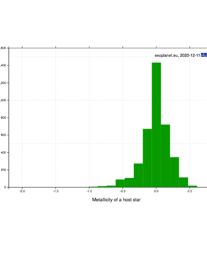
Figure 1: Frequency of planets in the Extrasolar Planets Encyclopedia database (exoplanet.eu) as a function of host star metallicity. Evidently the exoplanet frequency is similar to a Gaussian distribution centered on solar metallicity (0.0).

Ongoing observational work has shown that the strong dependence of exoplanet frequency on host star metallicity found by Fischer & Valenti (2005) has been supplanted by a nearly symmetrical frequency distribution centered on solar metallicity (Figure 1), weakening the overall case for exoplanet formation primarily by core accretion. Santos et al. (2017), Schlaufman (2018), Narang et al. (2018), Goda & Matsuo (2019), and Maldonado et al. (2019) all found that the distribution of exoplanet masses as a function of stellar metallicity depends on the exoplanet mass. Exoplanets with masses below $\sim 4M_{Jup}$ preferentially orbit high metallicity stars, while those with higher masses do not. Considering that core accretion is expected to be less efficient around low metallicity stars, as a consequence of a reduced feedstock for core assembly from planetesimals or pebbles, these studies imply that disk instability may be primarily responsible for the formation of the more massive exoplanets. Furthermore, Teske et al. (2019) did not find the clear correlation between host star metallicity and giant exoplanet excess metallicity that might be expected for formation by core accretion.

Core accretion has long had difficulty with forming gas giants around low mass, M dwarf stars (e.g., Laughlin et al. 2004), as opposed to the success of disk instability (e.g., Boss 2006). More recent work has confirmed the core accretion problem for low mass stars (Miguel et al. 2020), while M dwarfs still appear capable of forming gas giants by disk instability, provided their disks are massive enough (Mercer & Stamatellos 2020). The discovery of a gas giant planet orbiting the M5.5 dwarf star GJ 3512 has therefore been attributed to it having been formed by disk instability rather than by core accretion (Morales et al. 2019). High mass stars also appear to favor fragmentation as a formation process for their more massive companions (Cadman et al. 2020).

FU Ori-type stars undergo rapid luminosity increases that are consistently understood to be the result of a phase of gravitational instability and fragmentation (e.g., Takami et al. 2018). ALMA was used by Cieza et al. (2018) to show that FU Ori-type disks have radii less than 20 to 40 au and masses of 0.08 to 0.6 $M_{\odot}$, which are expected to be at least marginally gravitationally unstable. ALMA observations of the HL Tau disk have been used to interpret a disk gap as being caused by a gas giant planet in the process of formation by disk instability (Booth & Ilee 2020). ALMA disk gaps have been interpreted to be caused by embedded protoplanets with masses in the range of $\sim$ 0.1 to $\sim$ 10 $M_{Jup}$ at distances from $\sim$ 10 to $\sim$ 100 au (Zhang et al. 2018). ALMA imaging of the young stellar object BHB1 (Alves et al. 2020), with a disk gap, suggests that a massive gas giant planet has formed at the same time that the protostar is still accreting, i.e., at a very early age, less than 1 Myr. Four annular structures have been found by ALMA in a protostellar disk less than 0.5 Myr old (Segura-Cox et al. 2020), again implying rapid formation of protoplanets at large distances, presumably implicating disk gravitational instability. ALMA has also been used to study the spiral arms surrounding the AFGL 4176 O-type star, finding that the outer disk is cool enough to be gravitationally unstable and is likely to fragment into a companion object (Johnston et al. 2020). In fact, outer disk temperatures for the HD 163296 protoplanetary disk drop to $\sim$ 18 K in the midplane beyond 100 au (Dullemond et al. 2020). While disks with spiral arms appear to be rare, this may be more a result of spiral arm suppression by migrating giant planets than of insufficient mass for the disks to be gravitationally unstable (Rowther et al. 2020). When spiral arms do appear, they need not be caused by embedded planets, but rather may be direct manifestations of disk gas gravitational instability (Chen et al. 2021; Xie et al. 2021).

Boss (2017) adopted the $\beta$ cooling approximation for disk thermodynamics to study instabilities in disks with a wide range of $\beta$ values (1 to 100), starting with initial disks ranging from gravitationally unstable (Toomre $Q_{min}=1.3$) to gravitationally stable ($Q_{min}=2.7$), finding that fragmentation could occur for all $\beta$ values so long as the disks were initially close enough to instability ($Q_{min}<2$). Boss (2019) then addressed the question of evolving toward such an unstable configuration from an initially gravitationally stable configuration that is being cooled. Starting with $Q_{min}=2.7$ disks, but with the minimum disk temperature allowed to cool down to 40 K (equivalent to the outer disk temperature of models with initial $Q_{min}=1.3$), Boss (2019) found that fragmentation could still occur for the same wide range of $\beta$ values.

The present paper presents a suite of disk instability models that are variations on the $\beta$ cooling models of Boss (2019), now computed with as much as quadrupled spatial resolution of the spherical coordinate grid to avoid the need for the insertion of virtual protoplanets (VPs). The Boss (2019) models were restricted to a maximum of 200 radial ($r$) and 1024 azimuthal ($\phi$) grid points prior to VP insertion, whereas the new models double both of these maxima, up to 400 in radius and 2048 in azimuth (the vertical resolution was unchanged). These are the highest spatial resolution grid models ever run with the EDTONS code. However, this enhanced spatial resolution comes only with the severe penalty of running potentially eight times slower than the highest resolution models presented in Boss (2019). The factor of eight results from having the Courant time step halved and having four times as many grid points to compute at each time step. The new models are thus designed to learn to what extent the previous models might be considered to be close to having converged to the ideal of the continuum limit of infinite spatial resolution.

2 Numerical Methods and Initial Conditions

The code is the same as that used in many previous studies of disk instability by the author (e.g., Boss 2005, 2006, 2007, 2013, 2017, 2019). The EDTONS code solves the three-dimensional equations of hydrodynamics and the Poisson equation for the gravitational potential, with second-order-accuracy in both space and time, on a spherical coordinate grid (see Boss & Myhill 1992). The van Leer type hydrodynamic fluxes have been modified to improve stability (Boss 1997b). Numerous tests of the code are presented in Boss & Myhill (1992).

The energy equation is solved explicitly in conservation law form, as are the five other hydrodynamic equations. As in Boss (2017), the numerical code solves the specific internal energy $E$ equation (Boss & Myhill 1992):

$${\partial(\rho E)\over\partial t}+\nabla\cdot(\rho E{\bf v})=-p\nabla\cdot{\bf v}+L,$$

where $\rho$ is the gas density, $t$ is time, ${\bf v}$ is the velocity, $p$ is the gas pressure, and $L$ is the time rate of change of energy per unit volume, which is normally taken to be that due to the transfer of energy by radiation in the diffusion approximation. $L$ is defined in terms of the $\beta$ cooling formula (Gammie 2001), as follows. With $\beta=t_{cool}\Omega$, $t_{cool}$ is defined as the ratio of the specific internal energy to the time rate of change of the specific internal energy. $L$ is thus defined to be:

$$L=-{\rho E\Omega\over\beta},$$

where $\Omega$ is the local angular velocity of the gas. $L$ is always negative with this formulation, i.e., only cooling is permitted.

Detailed equations of state for the gas (primarily molecular hydrogen) and dust grain opacities are employed in the models; an updated energy equation of state is described by Boss (2007). The central protostar is effectively forced to wobble in order to preserve the location of the center of mass of the entire system (Boss 1998), which is accomplished by altering the apparent location of the point mass source of the star’s gravitational potential in order to balance the center of mass of the disk. No artificial viscosity is used in the models.

The numerical grid has $N_{r}=100$, 200, or 400 uniformly spaced radial grid points, $N_{\theta}=23$ theta grid points, distributed from $\pi/2\geq\theta\geq 0$ and compressed toward the disk midplane, and $N_{\phi}=512$, 1024, or 2048 uniformly spaced azimuthal grid points. The radial grid extends from 4 to 20 au, with disk gas flowing inside 4 au being added to the central protostar, whereas that reaching the outermost shell at 20 AU loses its outward radial momentum but remains on the active hydrodynamical grid. The $\theta$ grid points are compressed into the midplane to ensure The gravitational potential is obtained through a spherical harmonic expansion, including terms up to $N_{Ylm}=48$ for all spatial resolutions.

The $r$ and $\phi$ numerical resolution is doubled and then quadrupled when needed to avoid violating the Jeans length (e.g., Boss et al. 2000) and Toomre length criteria (Nelson 2006). As in Boss (2017, 2019), if either criterion is violated, the calculation stops, and the data from a time step prior to the criterion violation is used to double the spatial resolution in the relevant direction by dividing each cell into half while conserving mass and momentum. Here, however, the models can be doubled again to as high a spatial resolution as $N_{r}=400$ and $N_{\phi}=2048$ if needed. Even with this quadrupled spatial resolution, in one model (beq3) dense clumps formed that violated the Jeans or Toomre length criteria at their density maxima. In that case, the maximum density cell is again drained of 90% of its mass and momentum, which is then inserted into a virtual protoplanet (VP, Boss 2005), as in Boss (2017, 2019). The VPs orbit in the disk midplane, subject to the gravitational forces of the disk gas, the central protostar, and any other VPs, while the disk gas is subject to the gravity of the VPs. VPs gain mass at the rate (Boss 2005, 2013) given by the Bondi-Hoyle-Lyttleton (BHL) formula (e.g., Ruffert & Arnett 1994), as well as the angular momentum of any accreted disk gas. As in Boss (2017, 2019), VPs that reach the the inner or outer boundaries are simply tallied and removed from the calculation.

In the Boss (2017, 2019) models, the initial gas disk density distribution is that of an adiabatic, self-gravitating, thick disk with a mass of $M_{d}=0.091M_{\odot}$, in near-Keplerian rotation around a solar mass protostar with $M_{s}=1.0M_{\odot}$ (Boss 1993). The initial outer disk temperature was set to 180 K for all models, yielding an initial minimum value of the Toomre (1964) $Q$ gravitational stability parameter of 2.7, i.e., gravitationally stable, though the disks were allowed to cool down to as low as 40 K, as in Boss (2019). As in Boss (2017, 2019), the values of $\beta$ that were explored (see Table 1) were 1, 3, 10, 20, 30, 40, 50, and 100.

Gammie (2001) proposed that the outcome of a gas disk gravitational instability would depend on the parameter $\beta$, and suggested a critical value for fragmentation of $\beta_{cr}=3$. As a result, a critical value of $\beta_{cr}=3$ became the standard for predicting the outcome of the fragmentation process in protoplanetary disks. However, subsequent work by many groups (as summarized in Boss 2017, 2019) has questioned whether or not the value of $\beta_{cr}=3$ is a correct indicator for disk fragmentation, with other estimates of the true value ranging from $\beta_{cr}=10$ to $\beta_{cr}=30$, depending on the details of the numerical code used, such as numerical resolution and the artificial viscosity for smoothed-particle hydrodynamics (SPH) codes. More recently, Deng et al. (2017) found evidence for $\beta_{cr}=3$ for a novel meshless finite mass (MFM) code, but not for an SPH code, the latter apparently a result of artificial viscosity. Baehr et al. (2017) used local three-dimensional disk simulations to find $\beta_{cr}\sim 3$. Mercer et al. (2018) showed which of two approximate radiative transfer procedures is more accurate for protostellar disks, and demonstrated that the effective value of $\beta$ in such disks could vary from $\sim$ 0.1 to $\sim$ 200, i.e., a single, constant value of $\beta$ may not be capable of representing the full range of physical conditions in gravitationally unstable disks.

Boss (2017) discussed the problems of radiative transfer and cooling in disk instability calculations and the utility of the $\beta$ cooling approximation in sidestepping some of these issues. Boss (2001) calculated the first disk instability models with 3D radiative transfer hydrodynamics (RHD), finding that disk fragmentation was possible. Durisen et al. (2007) summarized much of the detailed work on 3D radiative transfer models, both from the side of models where clump formation occurred and from models where clump formation was less robust. While many numerical factors come to play in these calculations, e.g., grid resolutions for finite difference (FD) codes and smoothing lengths for SPH codes (e.g., Mayer et al. 2007), flux limiters for radiative transfer in the diffusion approximation, and accuracy of the gravitational potential solver, the key issue was determined to be whether a protoplanetary disk could remain sufficiently cold for spiral arms to form self-gravitating clumps that could contract toward planetary densities. Steiman-Cameron et al. (2013) studied the effect of spatial resolution on cooling times in RHD models, finding convergence for optically thick, inner regions, but not for optically thin, outer regions. Tsukamoto et al. (2015) used 3D RHD models to follow the formation of disks, starting from collapsing molecular cloud cores, finding that radiative heating from the interstellar medium could have a significant effect on the fragmentation process.

Note that as in the previous disk instability models in this series, magnetic fields can be neglected because of the low ionization levels in the optically thick disk midplanes (Gammie 1996; Boss 2005), where marginally gravitationally unstable disk dynamics occurs, at least for massive disks of the sizes (radii from 4 au to 20 au) considered here. Magnetic fields are expected to be of importance close to the protostar, at the disk surfaces, and at large distances from the protostar, especially in regions with strong EUV/FUV radiation from nearby O stars.

3 Results

The new models were started from the last saved time step of the model with corresponding $\beta$ in Boss (2019) before VPs were inserted, i.e., when the grids had only been doubled in $r$ and $\phi$, but not yet quadrupled. Table 1 lists the key results for all of the models: the final times reached, the number of VPs and of strongly (first number) or strongly and weakly (second number, when two numbers are given) gravitationally bound clumps present at the final time, the sum of those two ($N_{VP}$ + $N_{clumps}$ = $N_{total}$), and the number of VPs in Boss (2019) at the two time steps closest to the final time of the new models (a single number is given when both time steps have the same number of VPs). The number of clumps ($N_{clumps}$) was assessed by searching for dense regions with densities greater than $10^{-10}$ g cm^-3. For clumps of this density or higher, the free fall time is 6.7 yrs or less, considerably less than the orbital periods, implying that such clumps might be able to survive and contract to form gaseous protoplanets, provided there was sufficient spatial resolution. The orbital period of the disk gas at the inner edge (4 au) is 8.0 yr and 91 yrs at the outer edge (20 au). The final times reached ranged from 205 yrs to 326 yrs, indicating that the models spanned time periods long enough for many revolutions in the inner disk and multiple revolutions in the outer disk. The models required about 2.5 years to compute, with each model running on a separate, single core of the Carnegie memex cluster at Stanford University.

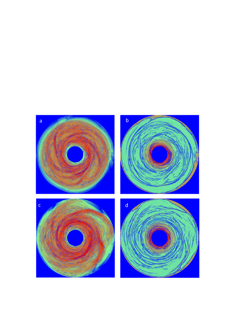
Figure 3: Equatorial (midplane) density (left) and temperature (right) contours for models beq5 (a,b) at 205 yrs and for model beq8 (c,d) at 326 yrs, respectively, plotted as in Figure 1. Maximum midplane gas densities are: (a) $1.2\times 10^{-9}$ g cm^-3 and (c) $6.2\times 10^{-10}$ g cm^-3.

The previous models with $\beta$ cooling (Boss 2017, 2019) all began from axisymmetric initial disks, and followed the growth of nonaxisymmetry as a result of disk self-gravitational instability, i.e., the formation and evolution of spiral arms and clumps, as shown in Figures 2 and 3 of Boss (2019). The present models all begin from the corresponding $\beta$ models of Boss (2019), just before the densest clumps were replaced with VPs, and so began highly nonaxisymmetric and clumpy. Figures 2 and 3 display the density and temperature distributions in the disk midplane for the eight new models with higher spatial resolution, showing the familiar proliferation of spiral arms and segments in both fields. As expected, the highest disk temperatures occur in the regions of highest disk density, where $\beta$ cooling is struggling to overcome the compressional heating of the disk gas in the clumps and arms.

In order to avoid violating the Jeans and Toomre length criteria during the evolutions, models beq1 through beq6 all required that the radial and azimuthal grids be doubled compared to the highest resolution used in the Boss (2019) models, that is, increased to the maximum values of $N_{r}=400$ and $N_{\phi}=2048$. In spite of these increases, model beq3 twice required the insertion of a VP in order to avoid violating the two length constraints, though only one VP was still active at the end of the calculation (Table 1). Models beq7 and beq8, on the other hand, only needed to be refined in radius in order to avoid the length criteria, and so reached a highest spatial resolution of $N_{r}=400$ and $N_{\phi}=1024.$ Given the slower $\beta$ cooling in models beq7 and beq8 than in the six lower $\beta$ models, this is to be expected. As in all the models in this series, the vertical resolution was fixed, with the theta grid cells compressed around the disk midplane for maximum vertical spatial resolution of the most dynamically evolving regions of the disk.

As noted above, Table 1 lists a range for the number of clumps present in the new models at the final time, with the range being the number of strongly or strongly and weakly gravitationally bound clumps, as defined below and in Table 2. Table 2 displays the clump properties for the eight new models upon which the numbers of clumps in Table 1 were assessed. The clumps are classified as either unbound (U), weakly (W), or strongly (S) self-gravitating, depending on whether the clump mass is less than (U), greater than (W), or more than 1.5 times (S) the Jeans mass for self-gravitational collapse. The Jeans mass is the mass of a sphere of uniform density gas with a radius equal to the Jeans length, where the Jeans length is the critical wavelength for self-gravitational collapse of an isothermal gas (e.g., Boss 1997b, 2005). In cgs units, the Jeans mass is given by $1.3\times 10^{23}(T/\mu)^{3/2}\rho^{-1/2}$, where $T$ is the gas temperature, $\rho$ the gas density, and $\mu$ the gas mean molecular weight. Clumps with masses exceeding the Jeans mass are capable of self-gravitational collapse on a time scale given by the free fall time. As previously noted, all of these clumps have a maximum density higher than $10^{-10}$ g cm^-3 (Table 2), implying collapse times shorter than a free fall time of 6.7 yr and thus shorter than their orbital periods.

An inspection of the last two columns in Table 1 shows that the total number of clumps and VPs formed in the present models ($N_{total}$) tracks reasonably well with the number of VPs ($N_{VP-2019}$) in the corresponding Boss (2019) models. The numbers in both cases drop from about 4 to 6 down to 1 to 2 as the $\beta$ parameter increases from 1 to 100, as to be expected as the cooling rate decreases. This result implies that the quadrupled spatial resolution of the present models, with the consequent major increase in computational times, does not appear to produce results that differ greatly from those obtained in the same disk model when the virtual protoplanet technique is employed to represent the highest density clumps.

The clump masses range from 0.30 $M_{Jup}$ to 2.3 $M_{Jup}$, i.e., from roughly a Saturn-mass to twice a Jupiter-mass. Table 3 lists the orbital parameters for the clumps displayed in Tables 1 and 2, based on their masses and midplane velocities at the final times shown in Table 1. Note that the maximum clump densities always occur in the midplane, except for a few clumps where the maximum occurs in the first cell above above the midplane, so the orbits summarized in Table 3 are all assumed to be restricted to the midplane, i.e., zero inclination.

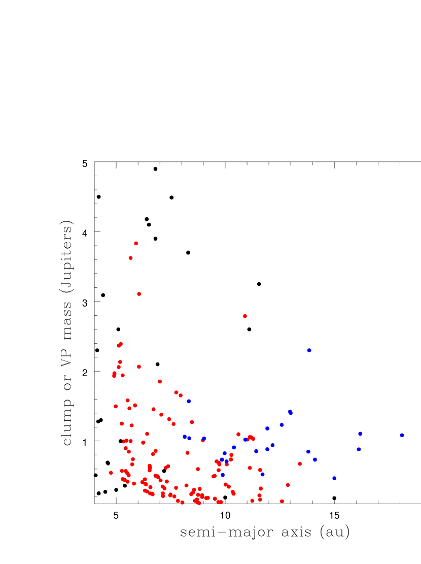
Figure 5: Same as Figure 4, except that now the red points show the VPs from the Boss (2019) models sampled at about 40 times during their evolutions, instead of only at the same time as the S and W clumps of the present models.

Figure 4 plots the clump masses for the present models as a function of semi-major axis, as well as the VPs from Boss (2019) at the data dump closest in time to the final times shown in Table 1. Note that the one VP that formed and survived in the present models (Table 1: model beq3) had a mass of only $4.3\times 10^{-3}$ $M_{Jup}$ and is not plotted in Figures 4 and 5. Also plotted in Figure 4 are the known exoplanets with masses and semi-major axes in the ranges of 0.1 $M_{Jup}$ to 5 $M_{Jup}$ and 4 au to 20 au, respectively. Figure 4 shows that the clumps formed primarily with semi-major axes in the range of 8 au to 16 au, whereas the VPs from Boss (2019) at those times orbited with semi-major axes between 6 au and 15 au. This slight discrepancy is due to the fact that once the VPs form, they orbit chaotically around the disk but with a tendency to move inward to smaller semi-major axes. This can be seen in Figure 5, where the VPs from Boss (2019) are shown not just at the same time as the clumps in Table 1, but at about 40 different data dumps, most of which show evolutionary times later than those plotted in Figure 4. Figure 5 shows that the VPs evolve to somewhat smaller semi-major axes on a time scale of a few hundred years (the Boss 2019 models ran as long as 462 yrs), and to some extent that inward evolution is responsible for the slight inward shift in semi-major axes compared to the clumps in Figure 4. The VPs also gain mass by BHL accretion rapidly over this time period, accounting for the much larger VP masses seen in Figure 5 compared to Figure 4, which is closer in time to when each VP was formed. The differing clump and VPs masses shown in Figure 4 are a result of the newly formed VPs having their mass derived solely from the single grid cell where the maximum density occurs, whereas the clump masses are derived by summing all the cells adjacent to the maximum density cell with densities no less than 0.1 that of the maximum density cell.

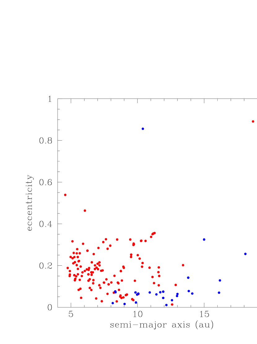
Figure 6: Eccentricities and semi-major axes for the clumps listed in Table 3 are shown in blue, while the red points show the values for the VPs from the Boss (2019) models sampled at about 40 times during their evolutions.

Figure 6 shows the semi-major axes and eccentricities for the VPs at multiple times and the clumps at their final time, again showing the inward migration of the VPs, as well as their eccentricities, which compare favorably in distribution to those of the clumps: most eccentricities are in the range of 0 to 0.35, but in both cases a few are as high as 0.9. Again, the quadrupled resolution clumps appear to support the VP model results in a broad sense.

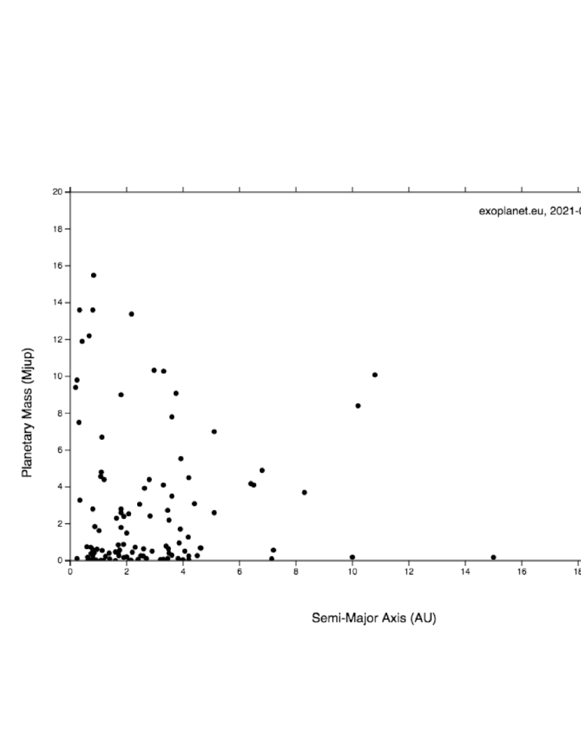
Figure 7: Masses and semi-major axes of the confirmed microlensing exoplanets listed in the Extrasolar Planets Encyclopedia (exoplanets.eu) for masses between 0.0 and 20 $M_{Jup}$ and semi-major axes between 0 au and 20 au.

While the goal of the present paper is to compare the quadrupled spatial resolution models with the VP models of Boss (2019), Figures 4 and 5 show that the observed exoplanets tend to have significantly higher masses and smaller semi-major axes than the clumps, though the agreement with the VPs is considerably better (see Table 2 in Boss 2019). Given that the observational biases for the known exoplanets favor large masses and small semi-major axes, the implication of the Boss (2019) and present models is that there may be a significant population of Jupiter-mass exoplanets orbiting from about 5 au to 15 au, awaiting discovery by future microlensing and direct imaging surveys (i.e., the Roman Space Telescope, RST). Figure 7 depicts the $\sim 100$ confirmed microlensing exoplanet discoveries to date, showing that a number of Jovian-mass exoplanets with semi-major axes between 5 au and 20 au have been detected by ground-based microlensing surveys, implying that they will be found in even greater numbers by the RST microlensing survey.

3.1 Discussion

Jin et al. (2020) undertook a semi-analytical model of the collapse of dense cloud cores to form protostars and protostellar disks. They found that disk fragmentation was most likely to occur at distances of 20 au to 200 au, though also at 200 au to 450 au to a reduced extent, with fragment masses expected primarily in the range of 3-35 $M_{Jup}$. Their disk model consists of a diffusion equation solution for the evolution of the gas surface density in an infinitely thin, one-dimensional (axisymmetric) disk, with fragmentation assumed to occur where the Toomre $Q$ value drops below 1.4. In their models, the Toomre $Q$ does not fall below 1.4 inside of 20 au, and so they do not predict any fragmentation to occur inside 20 au. Their models extend in time for about 1 Myr, by which time the typical disk extends well beyond 1000 au. In contrast, the present fully three dimensional gas hydrodynamics models do not attempt to follow the initial cloud core collapse phase (e.g., Boss 1982), but rather begin after protostar collapse has largely completed and left behind a 20 au radius, protoplanetary disk with an initial minimum Toomre $Q$ value of 2.7, stable with respect to fragmentation, and then follow the disk evolutions as they are allowed to cool.

4 Conclusions

These models have shown that increasingly higher spatial resolution models of the evolution of gravitationally unstable protoplanetary disks continue to support the possibility of the formation of self-gravitating clumps inside distances of 20 au from a solar-mass protostar. If these clumps are able to contract and survive their subsequent orbital evolution, they might imply the existence of a population of roughly Jupiter-mass exoplanets orbiting at distances that have not yet been thoroughly sampled by ground- or space-based telescopic surveys. The Roman Space Telescope, scheduled for launch in 2025, may be able to detect this largely unseen population through its gravitational microlensing survey, and perhaps may be able to perform direct imaging of a few with its coronagraphic instrument (CGI).

The fact that the quadrupled spatial resolution models produced results in terms of the number of clumps and of their initial orbital properties comparable to those of the virtual protoplanet (VP) models of Boss (2019) implies that the VP technique should be considered as a viable means for exploring a larger region of protoplanetary disk parameter space, as it yields comparable results with considerably lower computational burden than the quadrupled spatial resolution models presented here.

Clearly the utility of the $\beta$ cooling approximation needs to be further explored by comparison of the results of 3D RHD calculations with the results of 3D $\beta$ cooling models. A large set of such models is currently being calculated with the EDTONS code and will be the subject of a future publication. These new RHD models will also include quadrupled spatial resolution, in an attempt to test to what extent the models have approached convergence to the continuum limit, i.e., infinite spatial resolution.

The computations were performed on the Carnegie Institution memex computer cluster (hpc.carnegiescience.edu) with the support of the Carnegie Scientific Computing Committee. I thank Floyd Fayton for his invaluable assistance with the use of memex, and the referee for suggesting several additions to the manuscript.

Table 1: Results for the new models with varied $\beta$ cooling and quadrupled spatial resolution, showing the number of VPs and of clumps (both weakly and strongly gravitationally bound) at the final time, the sum of those two ($N_{VP}$ + $N_{clumps}$ = $N_{total}$), and the number of VPs in Boss (2019) at the two data dumps closest to the final time of the new models.

Model	$\beta$	final time (yrs)	$N_{VP}$	$N_{clumps}$	$N_{total}$	$N_{VP-2019}$
beq1	1	210.	0	4	4	5-6
beq2	3	206.	0	4-6	4-6	4-5
beq3	10	223.	1	3-5	4-6	3-4
beq4	20	267.	0	0-1	0-1	2
beq5	30	205.	0	1-2	1-2	3
beq6	40	245.	0	0-3	0-3	1
beq7	50	306.	0	1-2	1-2	1
beq8	100	326.	0	1-2	1-2	2

Table 2: Results for the new models, showing the estimated properties for the densest clumps present at the final times of the models, classified as either unbound (U), weakly (W), or strongly (S) self-gravitating, based on whether the clump mass is less than (U), greater than (W), or more than 1.5 times (S) the Jeans mass for self-gravitational collapse, with implications for clump survival.

Model	$\beta$	clump #	$\rho_{max}$ (g cm-3)	$M_{clump}$/$M_{Jup}$	$T_{average}$ (K)	$M_{Jeans}$/$M_{Jup}$	status
beq1	1	1	4.2e-10	0.51	106.	1.7	U
beq1	1	2	5.6e-10	2.3	44.	0.44	S
beq1	1	3	5.7e-10	0.83	47.	0.52	S
beq1	1	4	9.6e-10	1.0	43.	0.34	S
beq1	1	5	2.5e-9	0.94	42.	0.22	S
beq2	3	1	2.4e-9	1.0	102.	0.88	W
beq2	3	2	1.6e-9	1.6	92.	0.81	S
beq2	3	3	1.6e-9	1.4	51.	0.39	S
beq2	3	4	8.1e-10	1.2	42.	0.38	S
beq2	3	5	4.8e-10	1.4	42.	0.48	S
beq2	3	6	5.3e-10	0.71	44.	0.48	W
beq3	10	1	6.3e-9	0.91	86.	0.41	S
beq3	10	2	9.4e-10	0.52	41.	0.32	S
beq3	10	3	4.9e-10	1.1	44.	0.50	S
beq3	10	4	7.9e-10	0.47	45.	0.44	W
beq3	10	5	1.1e-9	0.32	115.	1.5	U
beq3	10	6	3.4e-10	0.85	52.	0.76	W
beq4	20	1	6.2e-10	0.48	56.	0.75	U
beq4	20	2	3.7e-10	0.85	54.	0.71	W
beq4	20	3	1.3e-9	0.53	69.	0.64	U
beq4	20	4	3.7e-10	0.33	53.	0.74	U
beq4	20	5	2.9e-10	0.78	57.	0.97	U
beq5	30	1	1.0e-9	0.73	45.	0.39	S
beq5	30	2	9.5e-10	0.51	52.	0.47	W
beq5	30	3	1.2e-9	0.30	54.	0.41	U
beq5	30	4	2.2e-10	0.55	47.	0.72	U
beq5	30	5	2.4e-10	0.48	53.	0.80	U
beq6	40	1	2.0e-9	1.1	99.	0.91	W
beq6	40	2	2.4e-10	0.45	48.	0.77	U
beq6	40	3	5.9e-10	0.72	65.	0.79	U
beq6	40	4	1.0e-9	0.73	67.	0.72	W
beq6	40	5	3.7e-10	1.1	57.	0.89	W
beq7	50	1	3.1e-10	0.88	48.	0.73	W
beq7	50	2	6.5e-10	0.88	55.	0.59	S
beq7	50	3	2.6e-10	0.47	47.	0.76	U
beq8	100	1	2.8e-10	1.2	48.	0.71	S
beq8	100	2	3.0e-10	0.66	63.	0.92	U
beq8	100	3	2.3e-10	0.51	48.	0.76	U
beq8	100	4	6.7e-10	1.0	60.	0.71	U

Table 3: Orbital parameters for the gravitationally bound clumps, i.e., those with a status of W or S in Table 2, at the final times listed in Table 1.

Model	$\beta$	clump #	semimajor axis (au)	eccentricity	status
beq1	1	2	13.85	0.078	S
beq1	1	3	9.97	0.061	S
beq1	1	4	10.92	0.071	S
beq1	1	5	12.17	0.011	S
beq2	3	1	8.35	0.072	W
beq2	3	2	8.33	0.076	S
beq2	3	3	12.95	0.064	S
beq2	3	4	11.93	0.045	S
beq2	3	5	12.97	0.054	S
beq2	3	6	10.06	0.066	W
beq3	10	1	10.42	0.856	S
beq3	10	2	11.71	0.072	S
beq3	10	3	18.09	0.256	S
beq3	10	4	14.99	0.325	W
beq3	10	6	13.81	0.142	W
beq4	20	2	11.42	0.062	W
beq5	30	1	14.11	0.066	S
beq5	30	2	9.88	0.023	W
beq6	40	1	8.14	0.020	W
beq6	40	4	9.85	0.071	W
beq6	40	5	16.19	0.129	W
beq7	50	1	16.12	0.070	W
beq7	50	2	11.93	0.075	S
beq8	100	1	12.59	0.034	S
beq8	100	4	9.03	0.016	U

Figure 2: Equatorial (midplane) density (left) and temperature (right) contours for models beq1 (a,b) at 210 yrs and for model beq3 (c,d) at 223 yrs, respectively. The disks have inner radii of 4 au and outer radii of 20 au. Density contours are labelled in log cgs units and temperature contours are labelled in log K units. Maximum midplane gas densities are: (a) $2.5\times 10^{-9}$ g cm^-3 and (c) $7.4\times 10^{-9}$ g cm^-3. The initial maximum midplane density is $1.0\times 10^{-10}$ g cm^-3 at 4 au. The models start with an initial minimum temperature of 180 K (light orange color) and can cool down to a minimum temperature of 40 K (light green color). The red color corresponds to temperatures of $\sim$ 1000 K.

Figure 4: Masses and semi-major axes of the S and W clumps from Table 3 are shown in blue, while the red points show the VPs from Boss (2019) at the data dump closest in time to the final times of the clumps listed in Table 1. The black points show all exoplanets listed in the Extrasolar Planets Encyclopedia (exoplanets.eu) for masses between 0.1 and 5 $M_{Jup}$ and semi-major axes between 4 au and 20 au.

References

- (1)
- (2) Alves, F. O., Cleeves, L. I., Girart, J. M., et al. ApJL, 904, L6
- (3)
- (4) Baehr, H., Klahr, H., & Kratter, K. M. 2017, ApJ, 848, 40
- (5)
- (6) Baron, F., Lafrenière, D., Artigou, E., et al. 2019, AJ, 158, 187
- (7)
- (8) Bohn, A. J., Kenworthy, M. A., Ginski, C., et al. 2020, ApJL, 898, L16
- (9)
- (10) Booth, A. S., & Ilee, J. D. 2020, MNRAS, 493, L108
- (11)
- (12) Boss, A. P. 1982, Icarus, 51, 623
- (13)
- (14) Boss, A. P. 1993, ApJ, 417, 351
- (15)
- (16) Boss, A. P. 1997a, Science, 276, 1836
- (17)
- (18) Boss, A. P. 1997b, ApJ, 483, 309
- (19)
- (20) Boss, A. P. 1998, ApJ, 503, 923
- (21)
- (22) Boss, A. P. 2001, ApJ, 563, 367
- (23)
- (24) Boss, A. P. 2005, ApJ, 629, 535
- (25)
- (26) Boss, A. P. 2006, ApJ, 643, 501
- (27)
- (28) Boss, A. P. 2007, ApJ, 661, L73
- (29)
- (30) Boss, A. P. 2013, ApJ, 764, 194
- (31)
- (32) Boss, A. P. 2017, ApJ, 836, 53
- (33)
- (34) Boss, A. P. 2019, ApJ, 884, 56
- (35)
- (36) Boss, A. P., & Myhill, E. A. 1992, ApJS, 83, 311
- (37)
- (38) Boss, A. P., Fisher, R. T., Klein, R. I., & McKee, C. F. 2000, ApJ, 528, 325
- (39)
- (40) Cadman, J., Rice, K., Hall, C., Haworth, T. J., & Biller, B. 2020, MNRAS, 492, 5041
- (41)
- (42) Chen, E., Yu, S.-Y., & Ho, L. C. 2021, ApJ, 906,19
- (43)
- (44) Cieza, L. A., Ruiz-Rodriquez, D., Perez, S., et al. 2018, MNRAS, 474, 4347
- (45)
- (46) Deng, H., Mayer, L., & Meru, F. 2017, ApJ, 847, 43
- (47)
- (48) Dullemond, C. P., Isella, A., Andrews, S. M., Skobleva, I., & Dzyurkevich, N. 2020, A&A, 633, A137
- (49)
- (50) Durisen, R. H., Boss, A. P., Mayer, L., Nelson, A., Rice, K., & Quinn, T. R. 2007, in Protostars and Planets V, B. Reipurth, D. Jewitt, & K. Keil, eds. (Tucson: University of Arizona Press), 607
- (51)
- (52) Fischer, D. A., & Valenti, J. 2005, ApJ, 622, 1102
- (53)
- (54) Gammie, C. F. 1996, Icarus, 457, 355
- (55)
- (56) Gammie, C. F. 2001, ApJ, 553, 174
- (57)
- (58) Goda, S., & Matsuo, T. 2019, ApJ, 876, 23
- (59)
- (60) Helled, R., Bodenheimer, P., Alibert Y., et al. 2014, in Protostars & Planets VI, eds. H. Beuther, R. Klessen, K. Dullemond, and Th. Henning, 643
- (61)
- (62) Jin, L., Liu, F., Jiang, T., Tang, P., & Yang, J. 2020, ApJ, 904, 55
- (63)
- (64) Johnston, K. G., Hoare, M. G., Beuther, H., et al. 2020, A&A, 634, L11
- (65)
- (66) Laughlin, G., Bodenheimer, P., & Adams, F. C. 2004, ApJ, 612, L73
- (67)
- (68) Maldonado, J., Villaver, E., Eiroa, C., & Micela, G. 2019, A&A, 624, A94
- (69)
- (70) Mayer, L., Lufkin, G., Quinn, T., & Wadsley, J. 2007, ApJ, 661, L77
- (71)
- (72) Mercer, A., & Stamatellos, D. 2020, A&A, 633, A116
- (73)
- (74) Mercer, A., Stamatellos, D., & Dunhill, A. 2018, MNRAS, 478, 3478
- (75)
- (76) Miguel, Y., Cridland, A., Ormel, C. W., Fortney, J. J., & Ida, S. 2020, MNRAS, 491, 1998
- (77)
- (78) Mizuno, H. 1980, Prog. Theor. Phys., 64, 544
- (79)
- (80) Morales, J. C., Mustill, A. J., Ribas, I., et al. 2019, Science, 365, 1441
- (81)
- (82) Narang, M., Manoj, P., Furlan, E., et al. 2018, AJ, 156, 221
- (83)
- (84) Nelson, A. F. 2006, MNRAS, 373, 1039
- (85)
- (86) Nielsen, E. L., De Rosa, R. J., Macintosh, B., et al. 2019, AJ, 158, 13
- (87)
- (88) Rowther, S., Meru, F., Kennedy, G. M., Nealon, R., & Pinte, C. 2020, ApJL, 904, L18
- (89)
- (90) Ruffert, M., & Arnett, D. 1994, ApJ, 427, 351
- (91)
- (92) Santos, N. C., Adibekyan, V., Figueira, P., et al. 2017, A&A, 603, A30
- (93)
- (94) Schlaufman, K. C. 2018, ApJ, 853, 37
- (95)
- (96) Segura-Cox, D. M., Schmiedeke, A., Pineda, J. E., et al. 2020, Nature, 586, 228
- (97)
- (98) Steiman-Cameron, T., Durisen, R. H., Boley, A. C., Michael, S., & McConnell, C. R. 2013, ApJ, 768
- (99)
- (100) Takami, M., Fu, G., Liu, H. B., et al. 2018, ApJ, 864, 20
- (101)
- (102) Teske, J. K., Thorngren, D., Fortney, J. J., Hinkel, N., & Brewer, J. M. 2019, AJ, 158, 239
- (103)
- (104) Toomre, A. 1964, ApJ, 139, 1217
- (105)
- (106) Tsukamoto, Y., Takahashi, S. Z., Machida, M. N., & Inutsuka, S. 2015, MNRAS, 446, 1175
- (107)
- (108) Xie, C., Ren, B., Dong, R., et al. 2021, ApJL, 906, L9
- (109)
- (110) Zhang, S., Zhu, Z., Huang, J., et al. 2018, ApJL, 869, L47
- (111)