Multi-task Learning by Leveraging the Semantic Information

Abstract

One crucial objective of multi-task learning is to align distributions across tasks so that the information between them can be transferred and shared. However, existing approaches only focused on matching the marginal feature distribution while ignoring the semantic information, which may hinder the learning performance. To address this issue, we propose to leverage the label information in multi-task learning by exploring the semantic conditional relations among tasks. We first theoretically analyze the generalization bound of multi-task learning based on the notion of Jensen-Shannon divergence, which provides new insights into the value of label information in multi-task learning. Our analysis also leads to a concrete algorithm that jointly matches the semantic distribution and controls label distribution divergence. To confirm the effectiveness of the proposed method, we first compare the algorithm with several baselines on some benchmarks and then test the algorithms under label space shift conditions. Empirical results demonstrate that the proposed method could outperform most baselines and achieve state-of-the-art performance, particularly showing the benefits under the label shift conditions.

Introduction

General machine learning paradigms typically focus on learning individual tasks. Even though significant progress has been achieved, recent successes in machine learning, especially in the deep learning area, usually rely on a large amount of labelled data to obtain a small generalization error. In practice, however, acquiring labelled data could be highly prohibitive, e.g., when classifying multiple objects in an image (Long et al. 2017), when analyzing patient data in healthcare data analysis (Wang and Pineau 2015; Zhou et al. 2021b), or when modelling users’ products preferences (Murugesan and Carbonell 2017). Data hungry has become a long-term problem for deep learning. Multi-task learning (MTL) aims at addressing this issue by simultaneously learning from multiple tasks and leveraging the shared knowledge across them. Many MTL approaches have been implemented in computer vision (Zhao et al. 2018), natural language processing (Bingel and Søgaard 2017), medical data analysis (Moeskops et al. 2016; Li, Carlson et al. 2018), brain-computer interaction (Wang et al. 2020) or cross-modality (Nguyen and Okatani 2019) learning problems. It has been shown with benefits to reduce the amount of annotated data per task to reach the desired performance.

The crucial idea behind MTL is to extract and leverage the knowledge and information shared across the tasks to improve the overall performances (Wang et al. 2019b), which can be achieved by task-invariant feature learning  (Maurer, Pontil, and Romera-Paredes 2016; Luo, Tao, and Wen 2017) or task relation learning (Zhang and Yeung 2012; Bingel and Søgaard 2017; Zhou et al. 2021b). One major issue with most of the existing feature learning approaches is that they only align the marginal distributions $\mathbb{P}(x)$ to extract the shared features without taking advantage of label information of the tasks. Consequently, the features can lack discriminative power for supervised learning even if their marginal features have been matched properly (Dou et al. 2019). Furthermore, only aligning $\mathbb{P}(x)$ cannot address the MTL problems when the label space of each task differs from each other, i.e., label shift problem (Redko et al. 2019).

While a few algorithms have been proposed to use semantic matching for MTL (Zhuang et al. 2017; Luo, Tao, and Wen 2017) and have shown improved performances, the theoretical justifications for the value of labels remain elusive. Most theoretical results (Shui et al. 2019; Mao, Liu, and Lin 2020) for MTL derive from the notion of $\mathcal{H}$-divergence (Ben-David et al. 2010) or Wasserstein adversarial training (Redko, Habrard, and Sebban 2017; Shen et al. 2018), which did not take the label information into consideration. As a result, they usually require additional assumptions, e.g., assuming the combined error across tasks is small (Ben-David et al. 2010) to ensure the algorithms succeed, which may not hold in practice.

To this end, we propose the first theoretical analysis for MTL that considers semantic matching. Specifically, our results reveal that the MTL loss can be upper-bounded in terms of the pair-wise discrepancy between the tasks, measured by the Jensen-Shannon divergences of label distribution $\mathbb{P}(y)$ and semantic distribution $\mathbb{P}(x|y)$.

The contributions of our work are trifold. 1. In contrast to previous theoretical results (Shui et al. 2019; Mao, Liu, and Lin 2020), which only consider the marginal distribution discrepancy (e.g., $\mathcal{H}$-divergence), we build a complete MTL theoretical framework upon the joint distribution discrepancy based on the Jensen-Shannon divergence. Thus, our result provides a deeper understanding of the general problem of MTL and insights into how to extract and leverage shared knowledge in a more appropriate and principled way by exploiting the label information. 2. Our analysis also reveals how the label shift problems affects the learning procedure of MTL, which was missing in previous results. 3. Our theoretical result leads to a novel algorithm, namely Semantic Multi-Task Learning (SMTL) algorithm, which explicitly leverages the label information for MTL.

Specifically, the proposed SMTL algorithm simultaneously learns task-invariant features and task similarities to match the semantic distributions across the tasks and minimizes label distribution divergence via a label re-weighting loss function. In addition, SMTL is based on a novel centroid matching approach for task-invariant feature learning, which is more efficient than other adversarial training based algorithms. To examine the effectiveness of the proposed algorithm, we evaluate SMTL on several benchmarks. The empirical results show that the proposed approach outperforms the baselines achieving state-of-the-art performance. Besides, the experiment results show that our algorithm can be more time-efficient than the adversarial baselines, which confirms the benefits of our proposed method. Furthermore, we also conduct a simulation of the label distribution shift scenario showing that the proposed algorithm could handle the label distribution shift problems that cannot be properly addressed by other baselines.

Related Works

Multi-task learning

MTL aims to learn multiple tasks simultaneously and improves learning efficiency by leveraging the shared features across tasks. It has been prevalent to lots of recent machine learning topics (Li, Liu, and Chan 2014; Wang, Pineau, and Balle 2016; Teh et al. 2017). Our work majorly relates to some feature representation learning-based approaches and task relation based approaches. (Maurer, Pontil, and Romera-Paredes 2016) firstly analyzed generalization error of representation-based approaches. (Murugesan et al. 2016; Pentina and Lampert 2017) approached the online and transductive learning problem by MTL using a weighted summation of the losses. (Wang et al. 2019a) analyzed the algorithmic stability in MTL. For task relations learning, (Zhang and Yeung 2010; Cao et al. 2018a) define a convex optimization problem to measure relationships while (Long et al. 2017; Kendall, Gal, and Cipolla 2018) propose probabilistic models by constructing task covariance matrices or estimate the multi-task likelihood via a deep Bayes model. Latterly, (Shui et al. 2019; Mao, Liu, and Lin 2020) combines the feature representation learning and task relations learning together and analyzed generalization bound under the adversarial training scheme motivated by the domain adaptation problems (Ben-David et al. 2010; Shen et al. 2018; Shui et al. 2020), showing improved performances in vision and language processing applications, respectively. This kind of approach neglected the value of label information, which may impair the learning process. There were also some approaches to investigate the situation where the label space may differ from each other.  (Su et al. 2020) investigate the problem where the task samples are confusing, and the model is trained to extract task concepts by discriminating them. These sample confusing concepts also have a connection with our semantic matching approach under the label distributions shift.

Semantic Transfer

Leveraging semantic information has been prevalent in some machine learning topics (Long et al. 2014), since it is easy to implement when few labels are available. Some few-shot adversarial based approaches (Motiian et al. 2017; Luo et al. 2017) have adopted the semantic alignment method for the learning scenario where a small amount of labelled data is available. (Dou et al. 2019; Zhou et al. 2021a; Matsuura and Harada 2020) proposed to leverage the semantic information by adopting the metric learning objective under an unsupervised scheme to enforce a class-specific alignment for domain generalization problems. (Zhang et al. 2019) propose to learn the class-specific prototype semantic information by a symmetric network to align semantic features for unsupervised domain adaptation problems.  (Xie et al. 2018) theoretically analyzed the semantic transfer method for domain adaptation problems with a pseudo label. (Shui et al. 2020) investigated the value of matching conditional and semantic distribution in domain adaptation problems. In the notion of MTL, leveraging the semantic information was investigated inconspicuously through some matrix decomposition methods in the notion of tensor learning. For example, (Zhuang et al. 2017) proposed a non-negative matrix factorization-based approach to learn a common semantic feature space underlying feature spaces of each task. (Luo, Tao, and Wen 2017) proposed to leveraging high-order statistics among tasks by analyzing the prediction weight covariance tensor of them. However, the theoretical analysis for leveraging the semantic information is still open.

Notations and Preliminaries

In this section, we start by introducing some necessary notations and preliminary problem setup.

Problem setup

Assuming a set of $T$ tasks $\{\hat{\mathcal{D}}_{t}\}_{t=1}^{T}$, each of them is generated by the underlying distribution $\mathcal{D}_{t}$ over $\mathcal{X}$ and by the underlying labelling functions $f_{t}:\mathcal{X}\to\mathcal{Y}$ for $\{(\mathcal{D}_{t},f_{t})\}_{t=1}^{T}$. A multi-task (MTL) learner aims to find $T$ hypothesis: $h_{1},\dots,h_{T}$ over the hypothesis space $\mathcal{H}$ to minimize the average expected error of all the tasks:

$$\arg\min_{h\in\mathcal{H}}\frac{1}{T}\sum_{i=1}^{T}\epsilon_{t}(h_{t}),$$

where $\epsilon_{i}(h_{i})\equiv\epsilon_{i}(h_{i},f_{i})=\mathbb{E}_{\mathbf{x}\sim\mathcal{D}_{i}}\ell(h_{i}(\mathbf{x}),f_{i}(\mathbf{x}))$ is the expected error of task $t$ and $\ell$ is the loss function. For each task $i$, assume that there are $m_{i}$ examples. For each task $i$, we consider a minimization of weighted empirical loss for each task by defining a simplex $\boldsymbol{\alpha}_{j}\in\Delta^{T}=\{\boldsymbol{\alpha}_{i,j}\geq 0,~{}\sum_{j=1}^{T}\boldsymbol{\alpha}_{i,j}=1\}$ for the corresponding weight for task $j$. It could be viewed as an explicit indicator of the task relations revealing how much information leveraged from other tasks.

The empirical loss $w.r.t.$ the hypothesis $h$ for task $i$ could be defined as,

$$\hat{\epsilon}_{\boldsymbol{\alpha}_{i}}(h)=\sum_{j=1}^{T}\boldsymbol{\alpha}_{i,j}\hat{\epsilon}_{j}(h),$$ (1)

where $\hat{\epsilon}_{i}(h)=\frac{1}{m_{i}}\sum_{j=1}^{m_{i}}\ell(h(x_{j}),y_{j})$ is the average empirical error for task $i$.

Most of the existing adversarial based MTL approaches, e.g. (Mao, Liu, and Lin 2020; Shui et al. 2019), were motivated by the theory of (Ben-David et al. 2010) using the $\mathcal{H}$ divergence. However, the $\mathcal{H}$-divergence theory itself is limited in many scenarios, e.g. when tackling the (semantic) conditional shifts and understanding open set learning problems (Panareda Busto and Gall 2017; Cao et al. 2018b; You et al. 2019). In this work, we adopt the Jensen-Shannon Divergence ($D_{\text{JS}}$) to measure the differences of tasks and analyze its potentials for controlling the semantic (covariate) relations i.e. measure the divergence between the tasks.

Definition 1 (Jensen-Shannon divergence).

Let $\mathcal{D}_{i}(x,y)$ and $\mathcal{D}_{j}(x,y)$ be two distribution over $\mathcal{X}\times\mathcal{Y}$, and let $\mathcal{M}=\frac{1}{2}(\mathcal{D}_{i}+\mathcal{D}_{j})$, then the Jensen-Shannon (JS) divergence between $\mathcal{D}_{i}$ and $\mathcal{D}_{j}$ is,

$$D_{\text{JS}}(\mathcal{D}_{i}\|\mathcal{D}_{j})=\frac{1}{2}[D_{\text{KL}}(\mathcal{D}_{i}\|\mathcal{M})+D_{\text{KL}}(\mathcal{D}_{j}\|\mathcal{M})]$$

where $D_{\text{KL}}(\mathcal{D}_{i}\|\mathcal{D}_{j})$ is the Kullback–Leibler divergence.

It has been prevalent in adversarial training based approaches in transfer learning (Dou et al. 2019; Matsuura and Harada 2020; Zhao et al. 2019). In practice, we could compute the Total Variation distance ($d_{TV}$) since it is an upper bound of JS divergence (Lin 1991):

$$d_{TV}(\mathcal{D}_{i}\|\mathcal{D}_{j})=\frac{1}{2}|\mathcal{D}_{i}-\mathcal{D}_{j}|$$ (2)

Leverage the semantic and label information

As aforementioned, previous MTL advancements (e.g. (Mao, Liu, and Lin 2020; Shui et al. 2019)) mostly only matched the marginal distribution while neglecting the labelling information. A successful MTL algorithm should take the semantic (covariate) conditional information into consideration. For example, consider the classification of different digits dataset (e.g. MNIST ($\mathcal{D}_{i}$) and SVHN $(\mathcal{D}_{j})$) using MTL, when conditioning on the certain digit category $Y=y$, it is clear that $\mathcal{D}_{i}(x|Y=y)\neq\mathcal{D}_{j}(x|Y=y)$, indicating the necessity of considering semantic information in MTL.

Moreover, a long-neglected issue in existing MTL approaches is that most MTL approaches all implicitly assumed that the label marginal distribution $\mathbb{P}(y)$ are the same. However, this may not hold. For example, in a medical diagnostics problem, if the data are collected from different hospitals with different populations in that area, the label spaces for data can vary from each other. Label shift refers to the situation where the source and target distribution have different label distribution (Redko et al. 2019), i.e., $D_{\text{JS}}(\mathcal{D}_{i}(y),\mathcal{D}_{j}(y))\neq 0$. While this issue has been investigated in literature by transfer learning (Panareda Busto and Gall 2017; Geng, Huang, and Chen 2020; Azizzadenesheli et al. 2019), however, the analysis towards label space shift in MTL is still open.

We show, both theoretically and empirically, that the label space shift can impair the MTL performance. Our theoretical and empirical results reveal that a successful multitask learning algorithm should not only match the semantic distribution $\mathcal{D}(x|y)$ among all the tasks via adversarial training with J-S divergence but also measure the label distribution $\mathcal{D}(y)$ under a re-weighting scheme for all tasks. Specifically, we consider the label distribution drift scenario, where the number of classes is the same to each other across the tasks while the number of instances in each class has obvious drift, i.e., imbalanced label distribution for all the tasks.

Methodology and Theoretical Insights

Intuitively, when aligning the distribution of different tasks, features from the same class should be mapped near to each other in the feature space satisfying the semantic conditional relations. We firstly analyze the error bound with the notion of Jensen-Shannon divergence based form to measure the tasks discrepancies. Then, we further extend the results to analyze to control the label space divergence and the semantic conditional distribution divergence. All the proofs are delegated to the supplementary materials.

Theorem 1.

Let $\mathcal{H}$ be the hypothesis class $h\in\mathcal{H}$. Suppose we have $T$ tasks generated by the underlying distribution and labelling function $\{(\mathcal{D}_{1},f_{1}),\dots,(\mathcal{D}_{T},f_{T})\}$. Assume the loss function $\ell$ is bounded by $L$ ($\max(\ell)-\min(\ell)\leq L$). Then, with high probability we have

$$\begin{split}\frac{1}{T}\sum_{t=1}^{T}\epsilon_{t}(h)&\leq\frac{1}{T}\sum_{t=1}^{T}\epsilon_{\alpha_{t}}(h)+\frac{\lambda_{0}}{4T}L^{2}\\ &+\frac{2}{\lambda_{0}T}\sum_{t=1}^{T}\sum_{i=1}^{T}\boldsymbol{\alpha}_{t,i}D_{\text{JS}}(\mathcal{D}_{t}(x,y)\|\mathcal{D}_{i}(x,y))\end{split}$$

where $\lambda_{0}>0$ is a constant.

Theorem 1 showed that the averaged MTL error is bounded by an averaged summation of all the tasks, the averaged summation of task distribution divergence among all pair of tasks and some constant value.

This bound indicates the joint distribution while we aim to leverage the label ($\mathbb{P}(y)$) and semantic ($\mathbb{P}(x|y)$) information, based on the aforementioned theorem 1, we could then decompose it into the following results,

Corollary 1.

Follow the setting of Theorem 1, we can further bound the overall task error by

$$\begin{split}\frac{1}{T}\sum_{t=1}^{T}\epsilon_{t}(h)&\leq\frac{1}{T}\sum_{t=1}^{T}\epsilon_{\alpha_{t}}(h)+\boldsymbol{\lambda}\underbrace{D_{\text{JS}}(\mathcal{D}_{t}(y)\|\mathcal{D}_{i}(y))}_{\text{Label distribution divergence}}\\ &+\boldsymbol{\lambda}\underbrace{\operatorname*{\mathbb{E}}_{y\sim\mathcal{D}_{t}(y)}D_{\text{JS}}(\mathcal{D}_{t}(x|y)\|\mathcal{D}_{i}(x|y))}_{\text{Semantic distribution divergence}}\\ &+\boldsymbol{\lambda}\underbrace{\operatorname*{\mathbb{E}}_{y\sim\mathcal{D}_{i}(y)}D_{\text{JS}}(\mathcal{D}_{t}(x|y)\|\mathcal{D}_{i}(x|y))}_{\text{Semantic distribution divergence}}+\frac{\lambda_{0}}{4T}L^{2}\end{split}$$

where $\boldsymbol{\lambda}\in\mathbb{R}^{T\times T}$ is the corresponding matrix whose $t$-th row and $i$-th column element is $\frac{2}{\lambda_{0}T}\sum_{t=1}^{T}\sum_{i=1}^{T}\boldsymbol{\alpha}_{t,i}$

Remark:

Different from (Shui et al. 2019; Mao, Liu, and Lin 2020), which were motivated by (Ben-David et al. 2010), our theoretical results do not rely on extra assumption of the existence of the optimal hypothesis to achieve a small combined error. Besides, our results also provide new insight by take advantage of label information and semantic conditional relations.

Corollary 1 implies that the averaged error over all tasks is bounded by the summation of task errors (the first term in R.H.S. of Corollary 1), the label distribution divergence (the second term), a constant term (the third term), and the semantic distribution divergence term (the last two terms). The first term could be easily optimized by a general supervised learning loss (e.g. the cross-entropy loss). To minimize this bound now is equivalent to match the semantic distribution among the tasks and measure the label divergence. Since the labels of each task samples are available to the learner, we could leverage the label and semantic information directly.

Algorithm 1 The Global Semantic Matching Method

Input: Training set from each tasks
Parameter: Feature extractor $\boldsymbol{\theta}^{f}$; decay parameter $\gamma$
Output: The semantic loss

1:  for k=1 to K do

2:     $C_{\mathcal{D}_{i}}^{k}\leftarrow\frac{1}{|\mathcal{D}_{i}^{k}|}\sum_{(x_{i},y_{i})\in\mathcal{D}_{i}^{k}}\boldsymbol{\theta}^{f}(x_{i})$

3:     $C_{\mathcal{D}_{j}}^{k}\leftarrow\frac{1}{|\mathcal{D}_{j}^{k}|}\sum_{(x_{j},y_{j})\in\mathcal{D}_{j}^{k}}\boldsymbol{\theta}^{f}(x_{j})$

4:     $\mathbf{C}_{\mathcal{D}_{i}}^{k}\leftarrow\gamma C_{\mathcal{D}_{i}}^{k}+(1-\gamma)C_{\mathcal{D}_{i}}^{k}$

5:     $\mathbf{C}_{\mathcal{D}_{j}}^{k}\leftarrow\gamma C_{\mathcal{D}_{j}}^{k}+(1-\gamma)C_{\mathcal{D}_{j}}^{k}$

6:     $\mathcal{L}_{S}\leftarrow\mathcal{L}_{S}+\Phi(C_{\mathcal{D}_{i}},C_{\mathcal{D}_{j}})$

7:  end for

8:  return $\mathcal{L}_{S}$

	3K				5K				8K
Approach	MNIST	MNIST-M	SVHN	Avg.	MNIST	MNIST-M	SVHN	Avg.	MNIST	MNIST-M	SVHN	Avg.
Vanilla	$93.9\pm 3.2$	$77.1\pm 2.6$	$57.3\pm 0.4$	$76.1$	$96.3\pm 1.2$	$79.1\pm 3.1$	$68.0\pm 2.9$	$81.1$	$97.7\pm 0.5$	$83.7\pm 2.2$	$71.4\pm 0.9$	$84.2$
Weighed	$89.3\pm 3.3$	$76.4\pm 3.1$	$70.2\pm 1.8$	$78.3$	$91.8\pm 2.7$	$74.2\pm 0.9$	$73.6\pm 3.1$	$79.8$	$92.3\pm 2.6$	$76.9\pm 3.1$	$74.1\pm 1.6$	$81.1$
Adv.H	$90.1\pm 1.2$	$\mathbf{81.2}\pm 1.3$	$70.8\pm 0.5$	$80.7$	$91.9\pm 2.6$	$\mathbf{83.7}\pm 1.4$	$73.6\pm 1.6$	$82.9$	$94.9\pm 1.6$	$\mathbf{85.2}\pm 0.3$	$79.1\pm 0.3$	$86.4$
Adv.W	$96.8\pm 0.6$	$81.3\pm 0.7$	$69.5\pm 1.1$	$82.5$	$97.5\pm 0.2$	$83.4\pm 0.4$	$72.6\pm 1.2$	$84.5$	$98.1\pm 0.3$	$84.3\pm 0.4$	$75.4\pm 1.1$	$86.1$
Multi-Obj.	$\mathbf{97.5}\pm 0.3$	$76.9\pm 0.5$	$54.8\pm 0.3$	$76.4$	$\mathbf{98.2}\pm 0.2$	$80.2\pm 0.7$	$61.2\pm 0.8$	$79.9$	$\mathbf{98.5}\pm 0.3$	$82.8\pm 0.5$	$69.9\pm 0.9$	$83.7$
AMTNN	$96.9\pm 0.2$	$80.8\pm 1.5$	$77.1\pm 0.9$	$84.9$	$97.7\pm 0.1$	$83.6\pm 1.1$	$78.4\pm 0.8$	$86.6$	$98.1\pm 0.2$	$83.1\pm 2.1$	$80.2\pm 1.3$	$87.1$
Ours	$95.4\pm 0.3$	$80.1\pm 0.5$	$\mathbf{81.5}\pm 0.6$	$\mathbf{85.7}$	$95.8\pm 0.3$	$82.4\pm 0.4$	$\mathbf{83.3}\pm 0.3$	$\mathbf{87.2}$	$96.0\pm 0.3$	$83.9\pm 0.4$	$\mathbf{85.4}\pm 0.2$	$\mathbf{88.4}$

Table 1: The empirical results (in $\%$) on the digits datasets.

Label Re-weighting Loss

Corollary 1 indicates that the error is also controlled by the label divergence term $D_{\text{JS}}(\mathcal{D}_{i}(y)\|\mathcal{D}_{j}(y))$. To reduce the influences caused by the label space shifts, we could adopt a label correction re-weighting loss (Lipton, Wang, and Smola 2018) based on the number of instances in each class,

$$\hat{\epsilon}^{\beta}_{\mathcal{D}_{i}}(h)=\sum_{(x_{i},y_{i})\in\hat{\mathcal{D}_{i}}}\boldsymbol{\beta}(y_{i})\ell(h(x_{i}),y_{i}))$$ (3)

where $\boldsymbol{\beta}\in\mathbb{R}^{K\times 1}$ is weight for each class, and $\boldsymbol{\beta}_{j}$ is the weight for class $y_{j}$. For task $i$ with total $m_{i}$ instances, the weight of class $k\in K$ ($K$ is the total number of classes) is computed by $\boldsymbol{\beta}_{k}=\sum\frac{|\#y=y_{k}|}{m_{i}}$. This re-weighting scheme guarantees the instances from different classes could have equal probability to be sampled when training the model, which re-weights the loss according to frequency of each class that occurs during training. By doing so, the learner will not neglect those classes who have fewer instances and therefore takes care of label drift.

Note: the coefficient $\boldsymbol{\beta}$ is computed for re-weighting the loss from each task while $\boldsymbol{\alpha}$ is a set of weights indicating the relations between each other, i.e. how much information leveraged from other tasks.

When training the model, we maintain the task specific loss $\mathcal{L}_{i}=\hat{\epsilon}^{\beta}_{\mathcal{D}_{i}}(h)$ and compute the total classification loss

$$\mathcal{L}_{C}=\sum_{i=1}^{T}\boldsymbol{\alpha}_{i}\hat{\epsilon}^{\beta}_{\mathcal{D}_{i}}(h)$$ (4)

Semantic matching and task relation update

To compute Eq. 4, we still need to estimate the task relation coefficients $\boldsymbol{\alpha}$. As it indicates the relations between tasks, we are not able to measure its value at the beginning. To a better estimation, we need to update the coefficient $\boldsymbol{\alpha}$ automatically during the training process. Through Corollary 1, we could solve the coefficients via an convex optimization as

$$\begin{split}\min_{\boldsymbol{\alpha}_{1},\dots,\boldsymbol{\alpha}_{T}}&\quad\mathcal{L}_{C}+\sum_{i,t=1}^{T}\boldsymbol{\alpha}_{t,i}\sum\nolimits_{y}(\hat{\mathcal{D}}_{i}(y)+\hat{\mathcal{D}}_{t}(y)))\mathbf{E}_{i,t}\\ &+\sum_{t=1}^{T}||\boldsymbol{\alpha}_{t}||_{2}\\ &\text{s.t.}\quad\sum_{t}\boldsymbol{\alpha}_{t}=1\end{split}$$ (5)

where $\mathbf{E}_{i,t}=D_{\text{JS}}\left(\hat{\mathcal{D}_{t}}(x|y)\|\hat{\mathcal{D}_{t}}(x|y)\right)$ is the empirical semantic distribution divergence.

To align the semantic distribution, we adopt the centroid matching method by computing the Euclidean distance between two centroids in the embedding space. Denote $C_{\mathcal{D}_{i}}^{k}$ and $C_{\mathcal{D}_{j}}^{k}$ by two feature centroids from class $k$ of distribution $\mathcal{D}_{i}$ and $\mathcal{D}_{j}$ respectively, it could be computed by,

$$\Phi(C_{\mathcal{D}_{i}}^{k},C_{\mathcal{D}_{j}}^{k})=||C_{\mathcal{D}_{i}}^{k}-C_{\mathcal{D}_{j}}^{k}||^{2}$$ (6)

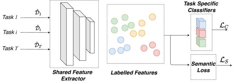
Figure 1: The overall model architecture

	$10\%$					$15\%$					$20\%$
Approach	A	C	P	S	avg.	A	C	P	S	avg.	A	C	P	S	avg.
Vanilla MTL	$78.8\pm 1.1$	$81.8\pm 1.4$	$87.1\pm 0.4$	$83.4\pm 0.6$	$82.8$	$82.8\pm 0.8$	$86.7\pm 0.9$	$89.3\pm 0.7$	$84.9\pm 0.7$	$85.9$	$84.1\pm 0.9$	$87.9\pm 0.8$	$90.5\pm 0.6$	$85.8\pm 1.2$	$87.1$
Weighted	$82.7\pm 1.1$	$86.2\pm 0.6$	$89.7\pm 1.1$	$84.9\pm 0.7$	$85.9$	$\mathbf{85.1}\pm 0.9$	$87.9\pm 0.7$	$91.2\pm 1.0$	$87.3\pm 0.7$	$87.9$	$86.1\pm 0.6$	$89.7\pm 0.4$	$92.1\pm 1.2$	$88.4\pm 0.9$	$89.1$
Adv.W	$78.8\pm 1.1$	$83.9\pm 1.2$	$87.6\pm 1.4$	$84.0\pm 0.9$	$83.6$	$83.6\pm 1.4$	$84.8\pm 0.5$	$84.7\pm 0.7$	$84.0\pm 0.6$	$84.2$	$83.5\pm 0.5$	$89.5\pm 0.7$	$91.4\pm 0.5$	$87.3\pm 0.6$	$87.9$
Adv.H	$76.8\pm 1.6$	$84.3\pm 0.4$	$88.3\pm 0.6$	$84.0\pm 0.6$	$83.3$	$82.6\pm 0.8$	$87.8\pm 0.7$	$89.9\pm 0.7$	$86.1\pm 0.4$	$86.6$	$84.4\pm 0.7$	$87.6\pm 0.3$	$91.5\pm 0.4$	$88.3\pm 0.4$	$87.9$
Multi-Obj.	$79.4\pm 1.8$	$83.4\pm 1.3$	$87.0\pm 0.5$	$82.9\pm 1.1$	$83.2$	$82.7\pm 0.5$	$87.5\pm 0.4$	$89.1\pm 0.6$	$86.5\pm 0.5$	$86.4$	$84.3\pm 0.9$	$88.7\pm 0.4$	$91.0\pm 0.3$	$88.8\pm 0.7$	$88.2$
AMTNN	$\mathbf{82.8}\pm 0.4$	$86.7\pm 0.4$	$91.3\pm 0.9$	$81.2\pm 0.8$	$85.5$	$85.1\pm 0.3$	$88.8\pm 0.3$	$92.9\pm 0.4$	$85.8\pm 0.5$	${88.2}$	$\mathbf{87.4}\pm 0.2$	$89.9\pm 0.6$	$93.7\pm 0.4$	$87.7\pm 0.1$	${89.7}$
Ours	$80.6\pm 0.4$	$\mathbf{87.9}\pm 0.4$	$\mathbf{94.4}\pm 0.5$	$\mathbf{91.9}\pm 0.5$	$\mathbf{88.9}$	$83.4\pm 0.4$	$\mathbf{89.8}\pm 0.6$	$\mathbf{94.5}\pm 0.4$	$\mathbf{93.1}\pm 0.4$	$\mathbf{90.2}$	$86.3\pm 0.3$	$\mathbf{91.6}\pm 0.4$	$\mathbf{95.5}\pm 0.4$	$\mathbf{93.8}\pm 0.4$	$\mathbf{91.8}$

Table 2: The empirical results (in %) on PACS dataset with AlexNet as feature extractor.

Our goal is to match the semantic distribution across tasks. For this, we re-visited the moving average centroid method by (Xie et al. 2018) where a global centroid matrix was maintained to compute the semantic information between a labeled source and an unlabeled target distribution for domain adaptation problem. Unlike (Xie et al. 2018), we could explicitly measure the semantic distribution across all the tasks rather than through assigning pseudo labels to compute them. We illustrate the modified moving average centroid method, namely The Global Semantic Matching Method in Algorithm. 1.

Remark:

Through Algorithm 1, the semantic loss $\mathcal{L}_{S}$ is an approximation of the total variation distance (see Eq. 2) of the two centroids, which is an upper bound of $\mathcal{D}_{\text{JS}}\left(\mathcal{D}_{i}(x|y),\mathcal{D}_{j}(x|y)\right)$. Compared with adversarial training based method, this semantic matching process does not need to train pair-wised discriminators, which may help to reduce the computational costs. For example, for $m$ tasks,  (Shui et al. 2019) needs to train $\frac{m(m-1)}{2}$ discriminators. When the number of tasks increase, the training procedure may become time-inefficient.

Algorithm 2 The proposed Semantic Multi-task learning algorithm

0:  Samples from different tasks $\{\hat{\mathcal{D}}_{t}\}_{t=1}^{T}$, initial coefficients $\{\boldsymbol{\alpha}_{t}\}_{t=1}^{T}$ and learning rate $\eta$

0:  Neural network $\boldsymbol{\theta}^{f}$, $\{\boldsymbol{\theta}_{t}^{C}\}_{t=1}^{T}$ and coefficient $\boldsymbol{\alpha}_{1},\dots,\boldsymbol{\alpha}_{T}$

1:  while Algorithm Not converge do

2:     for min-batch $\{(\mathbf{x}^{b}_{t},\mathbf{y}^{b}_{t})\}$ from task $\{\hat{\mathcal{D}}_{t}\}_{t=1}^{T}$ do

3:        Compute the classification objective $\mathcal{L}_{C}$ by Eq. 4

4:        Compute the semantic matching objective $\mathcal{L}_{S}$ via Algorithm 1

5:        Update the network parameters $\boldsymbol{\theta}^{f},\boldsymbol{\theta}^{c}_{t}$ by: $\boldsymbol{\theta}^{f}\leftarrow\boldsymbol{\theta}^{f}-\eta\frac{\partial\mathcal{L}_{C}+\mathcal{L}_{S}}{\partial\boldsymbol{\theta}^{f}}$ and $\boldsymbol{\theta}^{c}_{t}\leftarrow\boldsymbol{\theta}^{c}_{t}-\eta\frac{\partial\mathcal{L}_{C}+\mathcal{L}_{S}}{\partial\boldsymbol{\theta}^{c}_{t}}$

6:     end for

7:     Update $\{\boldsymbol{\alpha}_{t}\}_{t=1}^{T}$ by optimizing over Eq. (5).

8:  end while

The full objective and proposed algorithm

With the key components introduced in previous sections, we could summarize the full method. A general model architecture is provided in Fig. 1. The model learns multiple tasks jointly by a shared feature extractor. For each task, we implement a task-specific classifier. The classifier was trained under a re-weighting loss via measuring label distribution of each task, and we also maintain the semantic loss to match the semantic distribution across tasks to achieve the semantic transfer objective. The proposed Semantic Multi-task learning (SMTL) method is illustrated in Algorithm 2

Experiments and Analysis

Method	Amazon	Caltech	Dslr	WebCam	Average
Vanilla	$84.2\pm 1.1$	$80.6\pm 0.8$	$90.8\pm 2.3$	$81.8\pm 0.9$	$84.3$
Weighted	$88.1\pm 0.2$	$81.5\pm 0.9$	$94.9\pm 0.2$	$94.2\pm 0.5$	$88.6$
Adv.H	$81.5\pm 0.5$	$73.8\pm 1.8$	$91.4\pm 2.1$	$86.1\pm 1.4$	$83.3$
Adv.W	$84.9\pm 0.4$	$80.9\pm 0.9$	$94.5\pm 2.2$	$87.5\pm 1.5$	$86.9$
Multi-Obj.	$82.3\pm 0.7$	$76.7\pm 2.4$	$91.2\pm 1.7$	$86.8\pm 0.9$	$84.3$
AMTNN	$89.3\pm 0.9$	$84.3\pm 0.6$	$\mathbf{98.4}\pm 1.3$	$94.1\pm 0.7$	$91.7$
Ours	$\mathbf{90.9}\pm 0.4$	$\mathbf{85.3}\pm 0.5$	$98.1\pm 0.8$	$\mathbf{94.2}\pm 0.6$	$\mathbf{92.1}$

Table 3: Average test accuracy (in %) of MTL algorithms on Office-Caltech dataset with AlexNet as feature extractor.

	$5\%$				$10\%$				$20\%$
Approach	Amazon	Dslr	Webcam	avg.	Amazon	Dslr	Webcam	avg.	Amazon	Dslr	Webcam	avg.
Vanilla	$61.3\pm 1.3$	$71.8\pm 2.1$	$72.1\pm 1.1$	$68.3$	$73.2\pm 0.5$	$80.6\pm 1.4$	$82.1\pm 0.9$	$78.6$	$79.4\pm 0.8$	$91.2\pm 1.0$	$93.1\pm 0.8$	$87.9$
Weighted	$63.3\pm 0.2$	$87.4\pm 2.3$	$84.9\pm 0.6$	$78.5$	$70.6\pm 1.2$	$92.1\pm 0.9$	$88.4\pm 1.3$	$83.7$	$76.8\pm 0.9$	$\mathbf{96.6}\pm 0.7$	$95.6\pm 0.5$	$89.7$
Adv.W	$66.5\pm 1.9$	$71.8\pm 1.1$	$69.9\pm 0.9$	$69.7$	$74.7\pm 1.1$	$85.9\pm 0.8$	$85.7\pm 0.8$	$82.1$	$79.3\pm 0.6$	$93.8\pm 0.4$	$92.2\pm 0.9$	$88.4$
Adv.H	$65.8\pm 1.1$	$73.5\pm 0.8$	$71.4\pm 0.7$	$70.2$	$71.0\pm 0.9$	$84.1\pm 0.9$	$89.4\pm 0.1$	$81.4$	$79.7\pm 0.5$	$93.7\pm 0.7$	$93.7\pm 0.6$	$89.1$
Multi-Obj.	$\mathbf{68.9}\pm 1.2$	$72.5\pm 1.4$	$72.3\pm 0.4$	$71.3$	$74.6\pm 0.9$	$86.8\pm 1.1$	$86.9\pm 0.8$	$82.8$	$79.2\pm 0.8$	$92.1\pm 0.6$	$94.7\pm 0.6$	$88.6$
AMTNN	$63.3\pm 0.6$	$80.1\pm 1.6$	$85.4\pm 0.3$	$79.3$	$71.3\pm 1.2$	$\mathbf{92.8}\pm 0.9$	$89.6\pm 1.2$	$84.6$	$80.2\pm 0.9$	$94.2\pm 1.2$	$94.4\pm 0.9$	$89.6$
Ours	$68.5\pm 0.6$	$\mathbf{87.9}\pm 0.8$	$\mathbf{86.5}\pm 0.5$	$\mathbf{80.9}$	$\mathbf{75.7}\pm 0.2$	$\mathbf{92.8}\pm 0.2$	$\mathbf{90.8}\pm 0.3$	$\mathbf{86.4}$	$\mathbf{81.1}\pm 0.2$	$96.5\pm 0.1$	$\mathbf{96.1}\pm 0.2$	$\mathbf{91.2}$

Table 4: The empirical results (in %) on Office-31 dataset with ResNet-18 as feature extractor.

In order to investigate the effectiveness of our method, we examined the proposed approach comparing with several baselines on Digits, PACS (Li et al. 2017), Office-31 (Saenko et al. 2010), Office-Caltech (Gong et al. 2012) and Office-home (Venkateswara et al. 2017) dataset. For the Digits benchmark, we evaluate the algorithms on MNIST, MNIST-M and SVHN simultaneously. The PACS dataset, which was widely used in recent transfer learning researches, consists of images from four tasks: Photo (P), Art painting (A), Cartoon (C), Sketch (S), with objects from 7 classes. Office-31 dataset is a vision benchmark widely used in transfer learning related problems which consists of three different tasks: Amazon, Dslr and Webcam; Office-Caltech contains the 10 shared categories between the Office-31 dataset and Caltech256 dataset, including four different tasks: Amazon, Dslr, Webcam and Caltech; Office-home is a more challenging benchmark, which contains four different tasks: Art, Clipart, Product and Real World, with $65$ categories in each task.

	$5\%$					$10\%$					$20\%$
Approach	Art	Clipart	Product	Real-world	avg.	Art	Clipart	Product	Real-world	avg.	Art	Clipart	Product	Real-world	avg.
Vanilla	$26.2\pm 0.3$	$30.1\pm 0.2$	$57.6\pm 0.1$	$47.4\pm 1.1$	40.3	$35.8\pm 0.7$	$43.3\pm 0.6$	$67.1\pm 0.4$	$56.8\pm 1.3$	$50.7$	$45.5\pm 0.8$	$56.1\pm 0.6$	$74.4\pm 0.7$	$62.6\pm 0.6$	$59.6$
Weighted	$26.8\pm 1.6$	$31.8\pm 1.8$	$59.2\pm 0.4$	$50.5\pm 1.2$	$42.1$	$38.2\pm 1.0$	$45.3\pm 1.6$	$69.1\pm 0.2$	$58.3\pm 0.8$	$52.7$	$47.9\pm 0.1$	$56.7\pm 0.9$	$75.6\pm 0.6$	$64.8\pm 0.9$	$61.2$
Adv.W	$26.8\pm 0.8$	$32.7\pm 0.5$	$58.3\pm 0.9$	$47.1\pm 0.4$	$41.2$	$38.5\pm 0.8$	$44.4\pm 0.7$	$67.6\pm 0.7$	$59.5\pm 0.9$	$52.3$	$47.9\pm 0.5$	$56.7\pm 0.6$	$75.4\pm 1.1$	$65.7\pm 0.8$	$61.3$
Adv.H	$27.7\pm 1.4$	$32.1\pm 1.5$	$59.6\pm 0.7$	$51.1\pm 0.9$	$42.7$	$39.0\pm 0.9$	$45.8\pm 1.8$	$69.4\pm 0.4$	$58.8\pm 0.6$	$53.2$	$46.7\pm 0.5$	$56.5\pm 1.1$	$75.6\pm 0.4$	$65.1\pm 0.7$	$61.0$
Multi-Obj.	$25.6\pm 1.5$	$31.7\pm 1.7$	$58.7\pm 1.3$	$51.5\pm 0.9$	$41.8$	$34.6\pm 0.9$	$43.3\pm 1.4$	$66.1\pm 1.5$	$56.8\pm 0.7$	$50.2$	$46.2\pm 0.8$	$56.6\pm 0.5$	$74.3\pm 0.7$	$62.8\pm 0.6$	$59.8$
AMTNN	$32.5\pm 1.3$	$34.5\pm 0.9$	$56.3\pm 0.8$	$49.9\pm 1.8$	$43.3$	$41.1\pm 1.0$	$47.5\pm 0.8$	$68.4\pm 0.7$	$58.9\pm 0.9$	$53.9$	$48.9\pm 0.5$	$\mathbf{60.7}\pm 0.4$	$75.4\pm 0.4$	$64.7\pm 0.4$	$62.1$
Ours	$\mathbf{38.3}\pm 0.9$	$\mathbf{40.9}\pm 0.9$	$\mathbf{62.3}\pm 0.8$	$\mathbf{55.5}\pm 0.6$	$\mathbf{49.2}$	$\mathbf{43.8}\pm 0.6$	$\mathbf{50.4}\pm 0.8$	$\mathbf{71.3}\pm 0.9$	$\mathbf{62.3}\pm 0.6$	$\mathbf{57.1}$	$\mathbf{51.2}\pm 0.7$	$60.6\pm 0.8$	$\mathbf{77.9}\pm 0.4$	$\mathbf{66.1}\pm 0.6$	$\mathbf{64.3}$

Table 5: The empirical results (in %) on Office-home dataset with ResNet-18 as feature extractor.

Method	Amazon	Dslr	WebCam	Average
Cls. only	$79.4\pm 0.8$	$91.2\pm 1.0$	$93.1\pm 0.8$	$87.9$
$w.o.$ re-weighting	$80.2\pm 0.7$	$94.7\pm 1.3$	$94.1\pm 0.8$	$89.6$
$w.o.$ sem. matching	$79.8\pm 0.5$	$96.1\pm 0.3$	$95.4\pm 0.3$	$90.4$
$w.o.$ cvx opt.	$80.7\pm 0.3$	$\mathbf{96.8}\pm 0.5$	$95.3\pm 0.4$	$90.9$
Full method	$81.1\pm 0.2$	$96.5\pm 0.1$	$96.1\pm 0.2$	$\mathbf{91.2}$

Table 6: Ablation studies on Office-31 dataset.

To evaluate the performance of our proposed algorithm, we re-implement and compare our method with the following principled approaches:

• Vanilla MTL: Learning all the tasks simultaneously while optimizing the average summation loss: $\frac{1}{T}\sum_{t=1}^{T}\hat{\epsilon}_{t}(\boldsymbol{\theta}^{f},\boldsymbol{\theta}^{c}_{t})$, i.e., compute the loss uniformly.

• Weighted MTL: Adapted from (Murugesan et al. 2016), learning a weighted summation of losses over different tasks: $\frac{1}{T}\sum_{t=1}^{T}\hat{\epsilon}_{\boldsymbol{\alpha}_{t}}(\boldsymbol{\theta}^{f},\boldsymbol{\theta}^{c}_{t})$

• Adv.H: Adapted from (Liu, Qiu, and Huang 2017) by using the same loss function while training with $\mathcal{H}$-divergence as adversarial objective.

• Adv.W: Replace the adversarial loss of Adv.H by Wasserstein distance based adversarial training method.

• Multi-Obj.: Adapted from (Sener and Koltun 2018), casting the multi-task learning problem as a multi-objective problem

• AMTNN: Adapted from (Shui et al. 2019), a gradient reversal layer with Wasserstein adversarial training method.

Experiments on benchmark datasets

We first evaluate the MTL algorithms on Digits dataset. In order to show the effectiveness of MTL methods when dealing with small amount of labelled instances, we follow the evaluation protocol of (Shui et al. 2019) by randomly selecting $3k$, $6k$ and $8k$ instances of the training dataset and choose $1k$ dataset as validation set while testing one the full test set. For the SVHN dataset, we resize the images to $28\times 28\times 1$, except for that, we do not apply any data-augmentation towards to digits dataset. A LeNet-5 (LeCun et al. 1998) model is implemented as feature extractor and three 3-layer MLPs are deployed as task-specific classifiers, and extract the semantic feature from the classifier with size $128$. We adopt the Adam optimizer (Kingma and Ba 2014) for training the model from scratch. The model is trained for $50$ epochs while the initial learning rate is set by $1\times 10^{-3}$ and is decayed $5\%$ for every $5$ epochs. The results are reported in Table 1.

For the computer vision applications, we then test the SMTL algorithm comparing with the baselines on PACS and Caltech datasests using the AlexNet (Krizhevsky, Sutskever, and Hinton 2012) as feature extractor. For investigating the performance when limited amount labelled instances are available, we evaluate the algorithms on PACS dataset randomly select $10\%$, $15\%$ and $20\%$ of the total dataset for training, respectively. Since this Office-Caltech dataset is relatively small, we only test the dataset by using $20\%$ of the total images to train the model. We use the pre-trained AlexNet provided by PyTorch (Paszke et al. 2019) while removing the last FC layers as feature extractor (out feature size 4096). On top of the feature extractor, we implement several MLPs as task-specific classifiers. The test results are reported in Table 2 and Table 3, respectively. After that, we then evaluate the algorithms on Office-31 and Office-Home dataset by randomly select $5\%$, $10\%$ and $20\%$ training samples with pre-trained ResNet-18 model of PyTorch while removing the last FC layers as feature extractor (out feature size $512$). For these four vision benchmarks we follow the pre-processing and train/val/test protocol by (Long et al. 2017; Cao et al. 2018a; Li et al. 2017). We adopt the Adam optimizer with initial learning rate $2\times 10^{-4}$ and decayed $5\%$ every $5$ epochs while totally training for $80$ epochs. For stable training, we also enable the weight-decay in Adam optimizer to enforce a $L_{2}$ regularization. The test results are reported in Table 4 and 5, respectively. For more details about the experimental implementations, please refer to the supplementary materials.

From Table. 1$\sim$ 5, we could observe that our proposed method could outperform the baselines and improve the benchmark performances with state-of-the-art performances. Particularly, we found that when there are only few of labelled instances (e.g. $5\%$ of the total instances), our method could have a large margin of improvements regarding the baselines. This confirms the effectiveness of our methods when dealing with limited data.

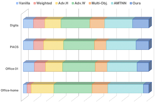
Figure 2: Relative time comparison (one training epoch) of the MTL algorithm on different benchmarks.

Further analysis

Ablation studies

In order to investigate the effectiveness of each component of our method, we conduct ablation studies (Table 6) of the proposed method on Office-31 dataset ($20\%$ of total instances) with four ablations, namely $1)$ Cls. only: remove all of the re-weighting scheme, semantic matching and the convex optimization towards updating $\boldsymbol{\alpha}$; $2)$ w.o. re-weighting: removing the re-weighting scheme inside the label weighting loss; $3)$ w.o. sem. matching: omitting the semantic matching; and $4)$ w.o. cvx. opt.: omit the optimization procedure for updating $\boldsymbol{\alpha}$, i.e, Eq. (5). The results showed that the label re-weighting scheme is crucial for the algorithm. Besides, we also observe $-1.0\%$ drop when omitting the semantic matching procedure and $-0.5\%$ once we omit the convex optimization procedure for $\boldsymbol{\alpha}$.

Time efficiency

As our method doesn’t rely on adversarial training, it has better time efficiency. We compare the time-efficiency of the MTL algorithms on Digits ($8k$), PACS ($20\%$), Office-31 ($20\%$) and Office-home ($20\%$) datasets, and report the time comparison of one training epoch in a relative percentage bar chart in Fig. 2. The adversarial based training methods (Adv.H, Adv.W and AMTNN) take longer time for a training epoch, especially on the Office-home dataset. Take the improved performance (Table 1$\sim$5) into consideration. Our method could improve that benchmark performance while reduce the time needed for training. This also demonstrates the benefits of algorithm in terms of time-efficiency.

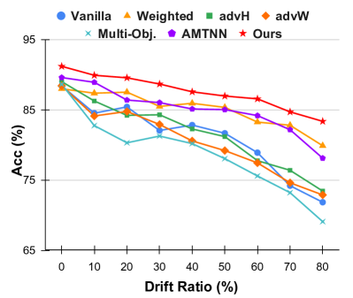
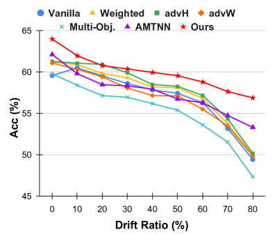
Figure 3: Performance comparison under label distribution drift scenario. Left: Evaluations on Office-31 dataset with different drift ratio; Right: Evaluations on Office-Home dataset with different drift ratio.

Performance under label shift

To confirm the effectiveness, we evaluate the MTL algorithms’ performance under label shift situation where the label distribution drifts, i.e., the number of classes keeps the same with original one while some classes drift by a certain percentage for a specific task on Office-31 and Office-home dataset. The drift simulation is implemented as keeping all the classes within all the tasks while simulating a significant label distribution drift by randomly drop out some part of the instances of certain tasks. For Office-31 dataset, the task Amazon’s class $1\sim 10$, task Dslr’s class $10\sim 20$ and task Webcam’s class $21\sim 30$ are drifted with different ratios ($10\%\sim 80\%$) while for Office-home dataset, we drift classes $1\sim 16$ of Art, classes $17\sim 32$ of Clipart, classes $33\sim 48$ of Product, and classes $49\sim 64$ of Real World with different ratios ($10\%\sim 80\%$).

We show the performance under label distribution drift ranging from $10\%\sim 80\%$ on Office-31 dataset (left) and on Office-Home dataset (right) in Fig. 3. As we could observe from Fig. 3, when the label space drifts, all the algorithms drop off. Our algorithm could outperform the baselines with a large margin when label space shift. This demonstrates the benefits of our algorithm for handling label shift problems.

Conclusion

We propose to leverage the labeling information across different tasks in multi-task learning problems. We first theoretically analyze the generalization bound of multi-task learning based on the notion of Jensen-Shannon divergence, which provides new insights into the value of label information by exploiting the semantic conditional distribution in multi-task learning. Our theoretical results also lead to a concrete algorithm that jointly matches the semantic distribution and controls label distribution divergence. The empirical results demonstrates the effectiveness of our algorithm on improving the benchmark performance with better time efficiency and particularly show the benefits when label distribution shift.

References

- Azizzadenesheli et al. (2019) Azizzadenesheli, K.; Liu, A.; Yang, F.; and Anandkumar, A. 2019. Regularized learning for domain adaptation under label shifts. arXiv preprint arXiv:1903.09734 .
- Ben-David et al. (2010) Ben-David, S.; Blitzer, J.; Crammer, K.; Kulesza, A.; Pereira, F.; and Vaughan, J. W. 2010. A theory of learning from different domains. Machine learning 79(1-2): 151–175.
- Bingel and Søgaard (2017) Bingel, J.; and Søgaard, A. 2017. Identifying beneficial task relations for multi-task learning in deep neural networks. In Proceedings of the 15th Conference of the European Chapter of the Association for Computational Linguistics: Volume 2, Short Papers, 164–169. Valencia, Spain: Association for Computational Linguistics. URL https://www.aclweb.org/anthology/E17-2026.
- Cao et al. (2018a) Cao, W.; Wu, S.; Yu, Z.; and Wong, H.-S. 2018a. Exploring Correlations Among Tasks, Clusters, and Features for Multitask Clustering. IEEE transactions on neural networks and learning systems 30(2): 355–368.
- Cao et al. (2018b) Cao, Z.; Ma, L.; Long, M.; and Wang, J. 2018b. Partial adversarial domain adaptation. In Proceedings of the European Conference on Computer Vision (ECCV), 135–150.
- Dou et al. (2019) Dou, Q.; de Castro, D. C.; Kamnitsas, K.; and Glocker, B. 2019. Domain generalization via model-agnostic learning of semantic features. In Advances in Neural Information Processing Systems, 6447–6458.
- Geng, Huang, and Chen (2020) Geng, C.; Huang, S.-j.; and Chen, S. 2020. Recent advances in open set recognition: A survey. IEEE Transactions on Pattern Analysis and Machine Intelligence .
- Gong et al. (2012) Gong, B.; Shi, Y.; Sha, F.; and Grauman, K. 2012. Geodesic flow kernel for unsupervised domain adaptation. In 2012 IEEE Conference on Computer Vision and Pattern Recognition, 2066–2073. IEEE.
- Kendall, Gal, and Cipolla (2018) Kendall, A.; Gal, Y.; and Cipolla, R. 2018. Multi-task learning using uncertainty to weigh losses for scene geometry and semantics. In Proceedings of the IEEE Conference on Computer Vision and Pattern Recognition, 7482–7491.
- Kingma and Ba (2014) Kingma, D. P.; and Ba, J. 2014. Adam: A method for stochastic optimization. arXiv preprint arXiv:1412.6980 .
- Krizhevsky, Sutskever, and Hinton (2012) Krizhevsky, A.; Sutskever, I.; and Hinton, G. E. 2012. Imagenet classification with deep convolutional neural networks. In Advances in neural information processing systems, 1097–1105.
- LeCun et al. (1998) LeCun, Y.; Bottou, L.; Bengio, Y.; Haffner, P.; et al. 1998. Gradient-based learning applied to document recognition. Proceedings of the IEEE 86(11): 2278–2324.
- Li et al. (2017) Li, D.; Yang, Y.; Song, Y.-Z.; and Hospedales, T. M. 2017. Deeper, broader and artier domain generalization. In Proceedings of the IEEE international conference on computer vision, 5542–5550.
- Li, Liu, and Chan (2014) Li, S.; Liu, Z.-Q.; and Chan, A. B. 2014. Heterogeneous multi-task learning for human pose estimation with deep convolutional neural network. In Proceedings of the IEEE conference on computer vision and pattern recognition workshops, 482–489.
- Li, Carlson et al. (2018) Li, Y.; Carlson, D. E.; et al. 2018. Extracting Relationships by Multi-Domain Matching. In Advances in Neural Information Processing Systems, 6799–6810.
- Lin (1991) Lin, J. 1991. Divergence measures based on the Shannon entropy. IEEE Transactions on Information theory 37(1): 145–151.
- Lipton, Wang, and Smola (2018) Lipton, Z. C.; Wang, Y.-X.; and Smola, A. 2018. Detecting and correcting for label shift with black box predictors. arXiv preprint arXiv:1802.03916 .
- Liu, Qiu, and Huang (2017) Liu, P.; Qiu, X.; and Huang, X. 2017. Adversarial multi-task learning for text classification. arXiv preprint arXiv:1704.05742 .
- Long et al. (2017) Long, M.; Cao, Z.; Wang, J.; and Philip, S. Y. 2017. Learning multiple tasks with multilinear relationship networks. In Advances in Neural Information Processing Systems, 1594–1603.
- Long et al. (2014) Long, M.; Wang, J.; Ding, G.; Sun, J.; and Yu, P. S. 2014. Transfer joint matching for unsupervised domain adaptation. In Proceedings of the IEEE conference on computer vision and pattern recognition, 1410–1417.
- Luo, Tao, and Wen (2017) Luo, Y.; Tao, D.; and Wen, Y. 2017. Exploiting High-Order Information in Heterogeneous Multi-Task Feature Learning. In IJCAI, 2443–2449.
- Luo et al. (2017) Luo, Z.; Zou, Y.; Hoffman, J.; and Fei-Fei, L. F. 2017. Label efficient learning of transferable representations acrosss domains and tasks. In Advances in Neural Information Processing Systems, 165–177.
- Mao, Liu, and Lin (2020) Mao, Y.; Liu, W.; and Lin, X. 2020. Adaptive Adversarial Multi-task Representation Learning. In International Conference on Machine Learning.
- Matsuura and Harada (2020) Matsuura, T.; and Harada, T. 2020. Domain Generalization Using a Mixture of Multiple Latent Domains. In AAAI.
- Maurer, Pontil, and Romera-Paredes (2016) Maurer, A.; Pontil, M.; and Romera-Paredes, B. 2016. The benefit of multitask representation learning. The Journal of Machine Learning Research 17(1): 2853–2884.
- Moeskops et al. (2016) Moeskops, P.; Wolterink, J. M.; van der Velden, B. H.; Gilhuijs, K. G.; Leiner, T.; Viergever, M. A.; and Išgum, I. 2016. Deep learning for multi-task medical image segmentation in multiple modalities. In International Conference on Medical Image Computing and Computer-Assisted Intervention, 478–486. Springer.
- Motiian et al. (2017) Motiian, S.; Jones, Q.; Iranmanesh, S.; and Doretto, G. 2017. Few-shot adversarial domain adaptation. In Advances in Neural Information Processing Systems, 6670–6680.
- Murugesan and Carbonell (2017) Murugesan, K.; and Carbonell, J. 2017. Active learning from peers. In Advances in Neural Information Processing Systems, 7008–7017.
- Murugesan et al. (2016) Murugesan, K.; Liu, H.; Carbonell, J.; and Yang, Y. 2016. Adaptive smoothed online multi-task learning. In Advances in Neural Information Processing Systems, 4296–4304.
- Nguyen and Okatani (2019) Nguyen, D.-K.; and Okatani, T. 2019. Multi-task learning of hierarchical vision-language representation. In Proceedings of the IEEE Conference on Computer Vision and Pattern Recognition, 10492–10501.
- Panareda Busto and Gall (2017) Panareda Busto, P.; and Gall, J. 2017. Open set domain adaptation. In Proceedings of the IEEE International Conference on Computer Vision, 754–763.
- Paszke et al. (2019) Paszke, A.; Gross, S.; Massa, F.; Lerer, A.; Bradbury, J.; Chanan, G.; Killeen, T.; Lin, Z.; Gimelshein, N.; Antiga, L.; et al. 2019. Pytorch: An imperative style, high-performance deep learning library. In Advances in neural information processing systems, 8026–8037.
- Pentina and Lampert (2017) Pentina, A.; and Lampert, C. H. 2017. Multi-task Learning with Labeled and Unlabeled Tasks. In International Conference on Machine Learning, 2807–2816.
- Redko, Habrard, and Sebban (2017) Redko, I.; Habrard, A.; and Sebban, M. 2017. Theoretical analysis of domain adaptation with optimal transport. In Joint European Conference on Machine Learning and Knowledge Discovery in Databases, 737–753. Springer.
- Redko et al. (2019) Redko, I.; Morvant, E.; Habrard, A.; Sebban, M.; and Bennani, Y. 2019. Advances in Domain Adaptation Theory. Elsevier.
- Saenko et al. (2010) Saenko, K.; Kulis, B.; Fritz, M.; and Darrell, T. 2010. Adapting visual category models to new domains. In European conference on computer vision, 213–226. Springer.
- Sener and Koltun (2018) Sener, O.; and Koltun, V. 2018. Multi-task learning as multi-objective optimization. In Advances in Neural Information Processing Systems, 527–538.
- Shen et al. (2018) Shen, J.; Qu, Y.; Zhang, W.; and Yu, Y. 2018. Wasserstein distance guided representation learning for domain adaptation. In Thirty-Second AAAI Conference on Artificial Intelligence.
- Shui et al. (2019) Shui, C.; Abbasi, M.; Robitaille, L.-E.; Wang, B.; and Gagné, C. 2019. A Principled Approach for Learning Task Similarity in Multitask Learning. In Proceedings of the Twenty-Eighth International Joint Conference on Artificial Intelligence, IJCAI-19.
- Shui et al. (2020) Shui, C.; Chen, Q.; Wen, J.; Zhou, F.; Gagné, C.; and Wang, B. 2020. Beyond -Divergence: Domain Adaptation Theory With Jensen-Shannon Divergence. arXiv preprint arXiv:2007.15567 .
- Su et al. (2020) Su, X.; Jiang, Y.; Guo, S.; and Chen, F. 2020. Task Understanding from Confusing Multi-task Data. In International Conference on Machine Learning.
- Teh et al. (2017) Teh, Y.; Bapst, V.; Czarnecki, W. M.; Quan, J.; Kirkpatrick, J.; Hadsell, R.; Heess, N.; and Pascanu, R. 2017. Distral: Robust multitask reinforcement learning. In Advances in Neural Information Processing Systems, 4496–4506.
- Venkateswara et al. (2017) Venkateswara, H.; Eusebio, J.; Chakraborty, S.; and Panchanathan, S. 2017. Deep Hashing Network for Unsupervised Domain Adaptation. In (IEEE) Conference on Computer Vision and Pattern Recognition (CVPR).
- Wang et al. (2019a) Wang, B.; Mendez, J.; Cai, M.; and Eaton, E. 2019a. Transfer learning via minimizing the performance gap between domains. In Advances in Neural Information Processing Systems, 10645–10655.
- Wang and Pineau (2015) Wang, B.; and Pineau, J. 2015. Online boosting algorithms for anytime transfer and multitask learning. In Twenty-Ninth AAAI Conference on Artificial Intelligence.
- Wang, Pineau, and Balle (2016) Wang, B.; Pineau, J.; and Balle, B. 2016. Multitask Generalized Eigenvalue Program. In AAAI, 2115–2121.
- Wang et al. (2020) Wang, B.; Wong, C. M.; Kang, Z.; Liu, F.; Shui, C.; Wan, F.; and Chen, C. P. 2020. Common Spatial Pattern Reformulated for Regularizations in Brain-Computer Interfaces. IEEE Trans. Cybern. doi:10.1109/TCYB.2020.2982901.
- Wang et al. (2019b) Wang, B.; Zhang, H.; Liu, P.; Shen, Z.; and Pineau, J. 2019b. Multitask metric learning: Theory and algorithm. In The 22nd International Conference on Artificial Intelligence and Statistics, 3362–3371. PMLR.
- Xie et al. (2018) Xie, S.; Zheng, Z.; Chen, L.; and Chen, C. 2018. Learning semantic representations for unsupervised domain adaptation. In International Conference on Machine Learning, 5423–5432.
- You et al. (2019) You, K.; Long, M.; Cao, Z.; Wang, J.; and Jordan, M. I. 2019. Universal domain adaptation. In Proceedings of the IEEE Conference on Computer Vision and Pattern Recognition, 2720–2729.
- Zhang et al. (2019) Zhang, Y.; Tang, H.; Jia, K.; and Tan, M. 2019. Domain-symmetric networks for adversarial domain adaptation. In Proceedings of the IEEE Conference on Computer Vision and Pattern Recognition, 5031–5040.
- Zhang and Yeung (2010) Zhang, Y.; and Yeung, D. Y. 2010. A convex formulation for learning task relationships in multi-task learning. In 26th Conference on Uncertainty in Artificial Intelligence, UAI 2010, Catalina Island, CA, United States, 8-11 July 2010, Code 86680.
- Zhang and Yeung (2012) Zhang, Y.; and Yeung, D.-Y. 2012. A convex formulation for learning task relationships in multi-task learning. arXiv preprint arXiv:1203.3536 .
- Zhao et al. (2019) Zhao, H.; Des Combes, R. T.; Zhang, K.; and Gordon, G. 2019. On Learning Invariant Representations for Domain Adaptation. In International Conference on Machine Learning, 7523–7532.
- Zhao et al. (2018) Zhao, X.; Li, H.; Shen, X.; Liang, X.; and Wu, Y. 2018. A modulation module for multi-task learning with applications in image retrieval. In Proceedings of the European Conference on Computer Vision (ECCV), 401–416.
- Zhou et al. (2021a) Zhou, F.; Jiang, Z.; Shui, C.; Wang, B.; and Chaib-draa, B. 2021a. Domain Generalization via Optimal Transport with Metric Similarity Learning. Neurocomputing doi:https://doi.org/10.1016/j.neucom.2020.09.091.
- Zhou et al. (2021b) Zhou, F.; Shui, C.; Abbasi, M.; Robitaille, L.-É.; Wang, B.; and Gagné, C. 2021b. Task Similarity Estimation Through Adversarial Multitask Neural Network. IEEE Transactions on Neural Networks and Learning Systems 32(2): 466–480. doi:10.1109/TNNLS.2020.3028022.
- Zhuang et al. (2017) Zhuang, F.; Li, X.; Jin, X.; Zhang, D.; Qiu, L.; and He, Q. 2017. Semantic feature learning for heterogeneous multitask classification via non-negative matrix factorization. IEEE transactions on cybernetics 48(8): 2284–2293.