OpenPifPaf:
Composite Fields for Semantic Keypoint Detection and Spatio-Temporal Association

Abstract

Many image-based perception tasks can be formulated as detecting, associating and tracking semantic keypoints, e.g., human body pose estimation and tracking. In this work, we present a general framework that jointly detects and forms spatio-temporal keypoint associations in a single stage, making this the first real-time pose detection and tracking algorithm. We present a generic neural network architecture that uses Composite Fields to detect and construct a spatio-temporal pose which is a single, connected graph whose nodes are the semantic keypoints (e.g., a person’s body joints) in multiple frames. For the temporal associations, we introduce the Temporal Composite Association Field (TCAF) which requires an extended network architecture and training method beyond previous Composite Fields. Our experiments show competitive accuracy while being an order of magnitude faster on multiple publicly available datasets such as COCO, CrowdPose and the PoseTrack 2017 and 2018 datasets. We also show that our method generalizes to any class of semantic keypoints such as car and animal parts to provide a holistic perception framework that is well suited for urban mobility such as self-driving cars and delivery robots.

I Introduction

The computer vision community has made tremendous progress in solving fine-grained perception tasks such as human body joints detection and tracking [1, 2]. We can cast these tasks as detecting, associating and tracking semantic keypoints. Examples of semantic keypoints are “left shoulders”, “right knees” or the “left brake lights of vehicles” as opposed to keypoints used in classical feature detectors that focus on the local geometry of the pixel intensities, like “corners” and “edges”. However, the performance of semantic keypoint tracking in live video sequences has been limited in accuracy and high in computational complexity and prevented applications to the transportation domain with real-time requirements like self-driving cars and last-mile delivery robots. The majority of self-driving car accidents is caused by “robotic” driving where the self-driving car conducts an allowed but unexpected stop and a human driver crashes into the self-driving car [3]. At their core, self-driving cars lack social intelligence. They are blind to the body language of surrounding pedestrians when every person is only perceived as a bounding box. Current pose detection and tracking methods are neither fast enough nor robust enough to occlusions to be viable for self-driving cars. Tracking human poses in real-time will enable self-driving cars to develop a finer-grained understanding of pedestrian behavior and with that a better conditioned reasoning for more natural driving.

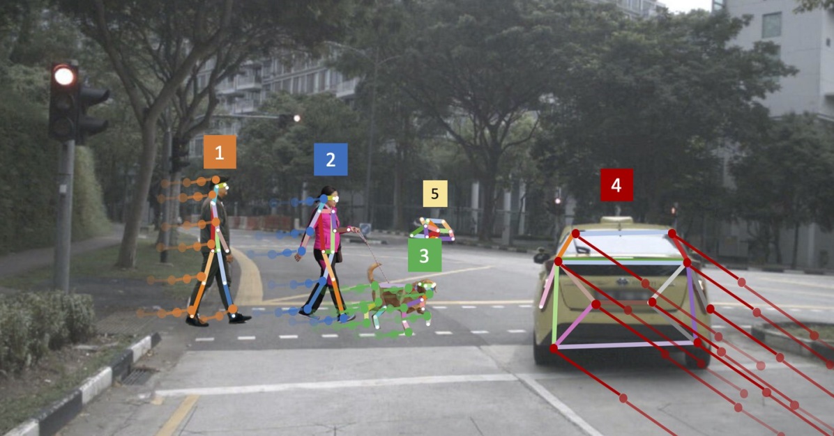
Figure 1: A real-world scene from the perspective of a self-driving car. Schematically, all moving actors are detected with their poses and tracked so that they can be consistently quantified over time. We place particular emphasis on understanding humans but also show generalizations to animals and cars. Here, a car (tracked as 4) is running a red light while also swerving to the right to avoid a woman (tracked as 2) who is walking her dog (tracked as 3).

The problem is to estimate and track multiple human, car and animal poses in image sequences, see Figure 1. The major challenges for tracking poses from the car perspective are (i) occlusions due to the viewing angle and (ii) prediction speed to be able to react to real-time changes in the environment. Our method must be fast enough to be viable for self-driving cars and robust to real-world variations like lighting, weather and occlusions.

Although tracking has been studied extensively before human pose estimation [4, 5, 6, 7], a significant cornerstone that leverages poses are the works of Insafutdinov et al. [8] and Iqbal et al. [9] who pioneered multi-person pose tracking for an arbitrary number of people in the wild. Both methods use graph matching to track independent, single-frame poses over time. To improve the matching for tracking, Doering et al. [10] introduced temporal flow fields that improve the cost function for matching. However, these works treat pose tracking as a multi-stage process: infer single-frame poses – which is itself a multi-stage process for top-down methods – and connect poses from frame to frame. This prohibits any improvement to single-frame poses that could result from the temporal information available in tracking. Here, we address these challenges by introducing a new method that jointly solves pose detection and tracking with Composite Fields.

First, we review Composite Fields for single-image multi-person pose estimation [11]. Second, we introduce a new method for pose tracking. While single-frame pose estimation can be viewed as a pose completion task starting at a seed joint, we treat pose tracking as a pose completion task starting with a pose from a previous frame and completing a spatio-temporal pose, which is a single, connected graph that spans space and time. The spatio-temporal pose consists of at least two single-frame poses and additional connections across the frames.

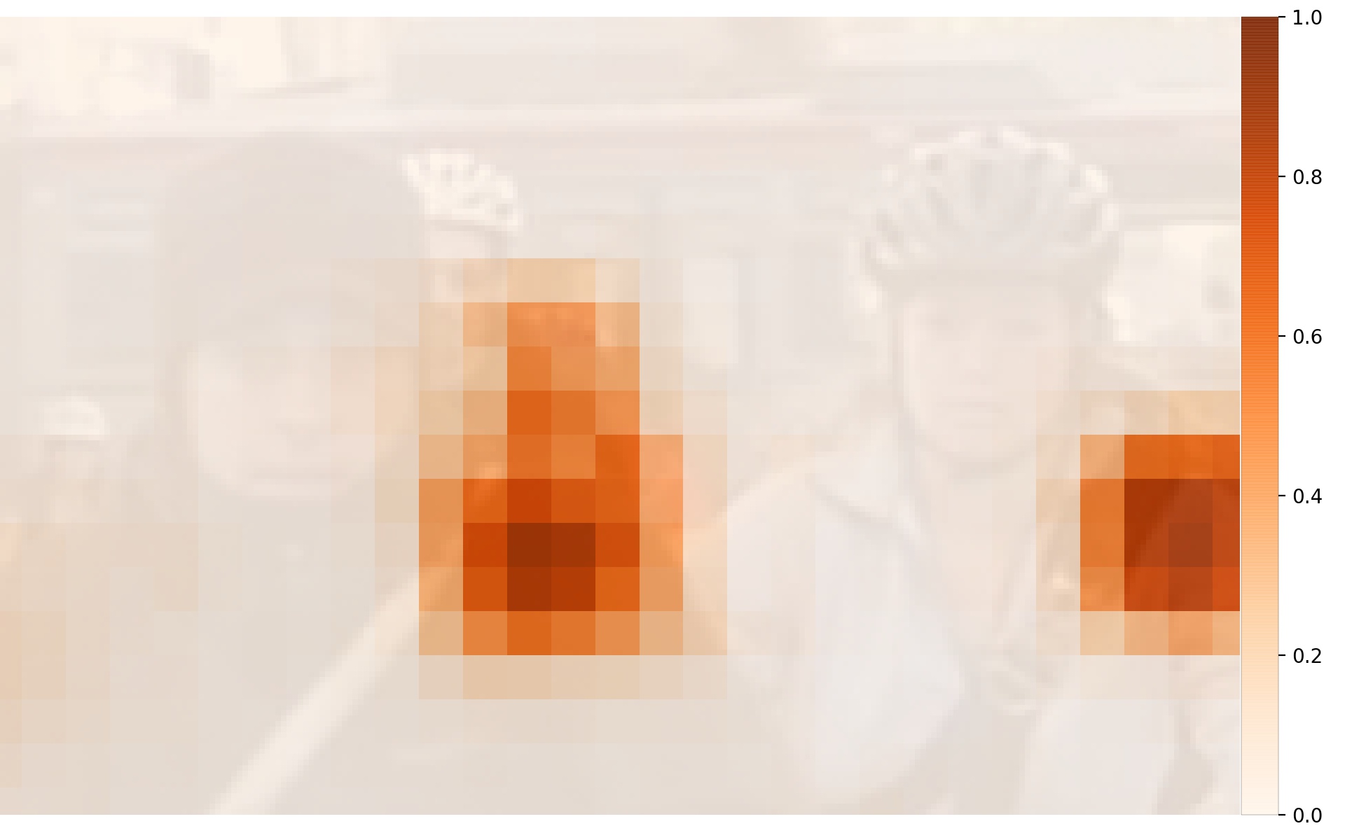
(a)

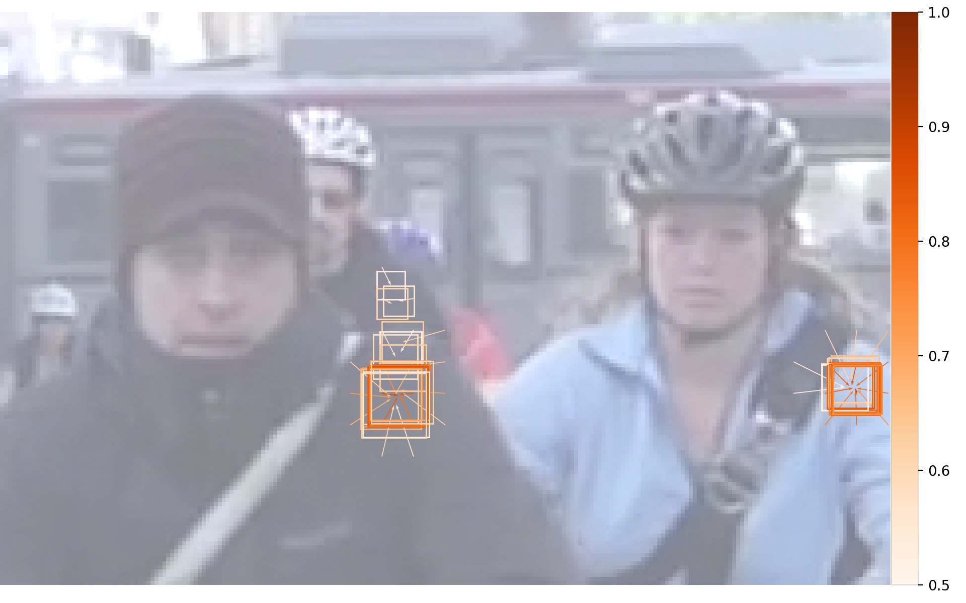
(b)

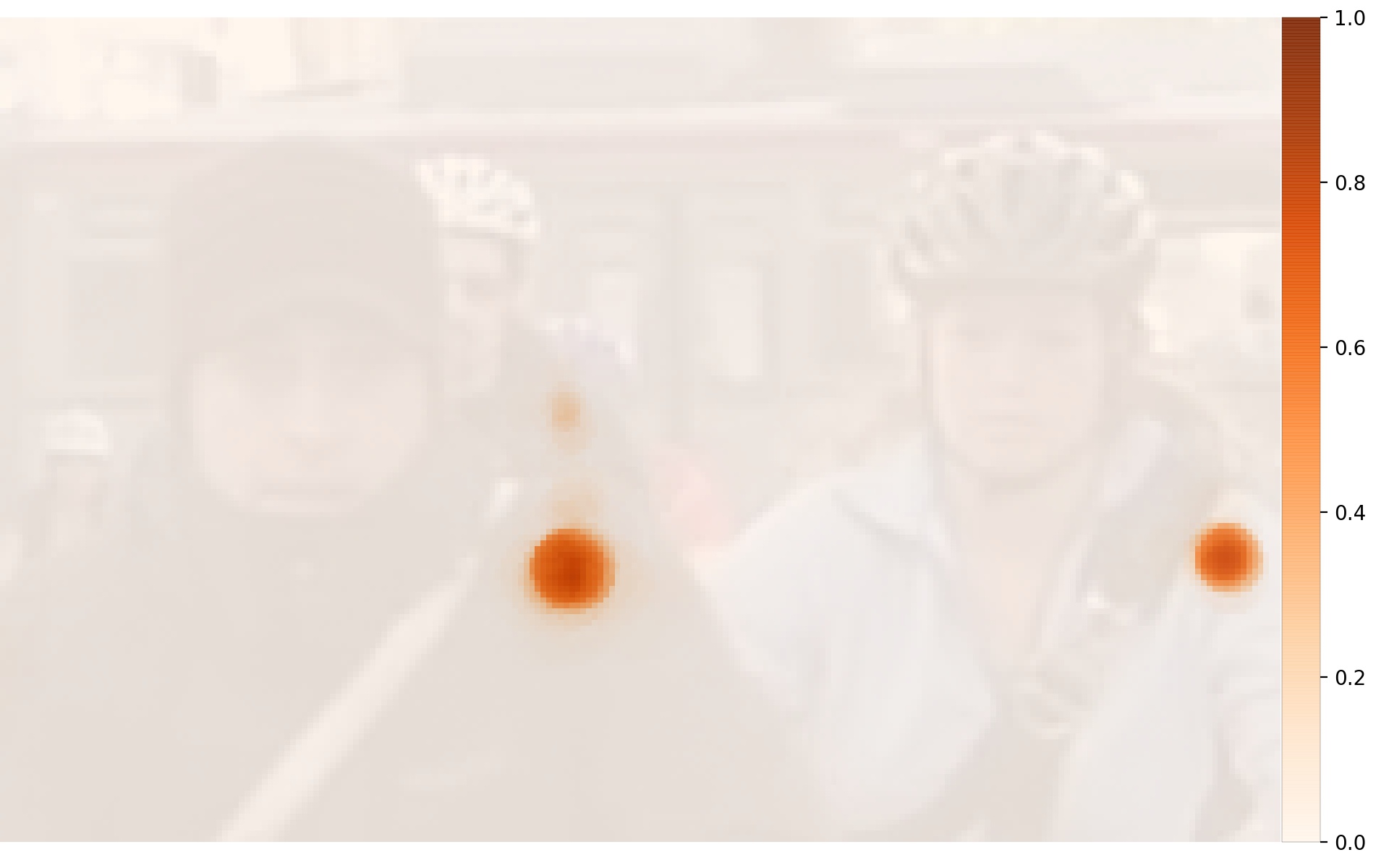
(c)

Figure 2: Visualizing the components of the CIF for the “left shoulder” keypoint on a small image crop. The confidence map is shown in (2a). The vector field with joint-scale estimates is shown in (2b). Only locations with confidence $>0.5$ are drawn. The fused confidence, vector and scale components according to Equation 1 are shown in (2c).

The contributions of this paper are (i) a Temporal Composite Association Field (TCAF) which we use to form a spatio-temporal pose and (ii) a greedy decoder to jointly detect and track poses. To the best of our knowledge, this method is the first single-stage, bottom-up pose detection and tracking method. We outperform all previous methods in accuracy and speed on the CrowdPose dataset [12] with its particularly crowded images. We perform on par with the state-of-the-art bottom-up method for single-image human pose estimation on the COCO [2] keypoint task in precision and are an order of magnitude faster in speed. Our model performs on par with the state-of-the-art method for human pose tracking on PoseTrack 2017 and 2018 [13] while simultaneously being an order of magnitude faster during prediction. We also show that our method generalizes to car and animal poses which demonstrates its suitability for a holistic perception framework. Our method is implemented as an open source library, referred to as OpenPifPaf.

II Related Work

II-A Pose Estimation

State-of-the-art methods for pose estimation are based on Convolutional Neural Networks [14, 15, 16, 17, 18, 19, 20, 21, 22, 23, 24]. All approaches for human pose estimation can be grouped into bottom-up and top-down methods. The former estimates each body joint first and then groups them to form a unique pose. The latter runs a person detector first and estimates body joints within the detected bounding boxes. Bottom-up methods were pioneered, e.g., by Pishchulin et al. with DeepCut [25]. In their work, the part association is solved with an integer linear program leading to processing times for one image of the order of hours. Newer methods use greedy decoders in combination with additional tools to reduce prediction time as in Part Affinity Fields [16], Associative Embedding [17], PersonLab [18] and multi-resolution networks with associate embedding [24]. PifPaf [11] introduced composite fields for pose estimation that produces a more precise association between joints than OpenPose’s Part Affinity Fields [16] and PersonLab’s mid-range fields [18]. In the next section, we will review composite fields and show that they generalize to tracking tasks.

II-B Pose Tracking

Tracking algorithms can be grouped into top-down versus bottom-up approaches for the pose part and the tracking part. Doering et al. [10] were the first to introduce a method that is bottom-up in both the spatial and the temporal part. They employ Part Affinity Fields [16] for the single-frame poses in a Siamese architecture. The temporal flow fields (TFF) feed into an edge cost computation for bipartite graph matching for tracking. The idea is extended in MIPAL [26] for tracking limbs instead of joints and in STAF [27].

Early work on multi-person pose tracking started with [8, 9]. Recent work has shown excellent performance on the PoseTrack 2018 dataset including the top-down method openSVAI [28] which decomposes the problem into three independent stages of human candidate detection, single-image human pose estimation and pose tracking. Similarly, LightTrack [29] also builds a strong top-down pipeline with interchangeable and independent modules. Miracle [30] uses a strong single-image pose estimator with a cascaded pyramid network together with an IOU tracker. HRNet for human pose estimation [20] leverages a multi-resolution backbone to produce high resolution feature maps that are context aware via HRNet’s multi-scale fusion. In MSRA/FlowTrack [19], optical flow is used to improve top-down tracking of bounding boxes for tracking of human poses. Pose-Guided Grouping (PGG) [31] proposes a part association method based on separate spatial and temporal embeddings. KeyTrack [32] uses pose tokenization and a transformer network to associate poses.

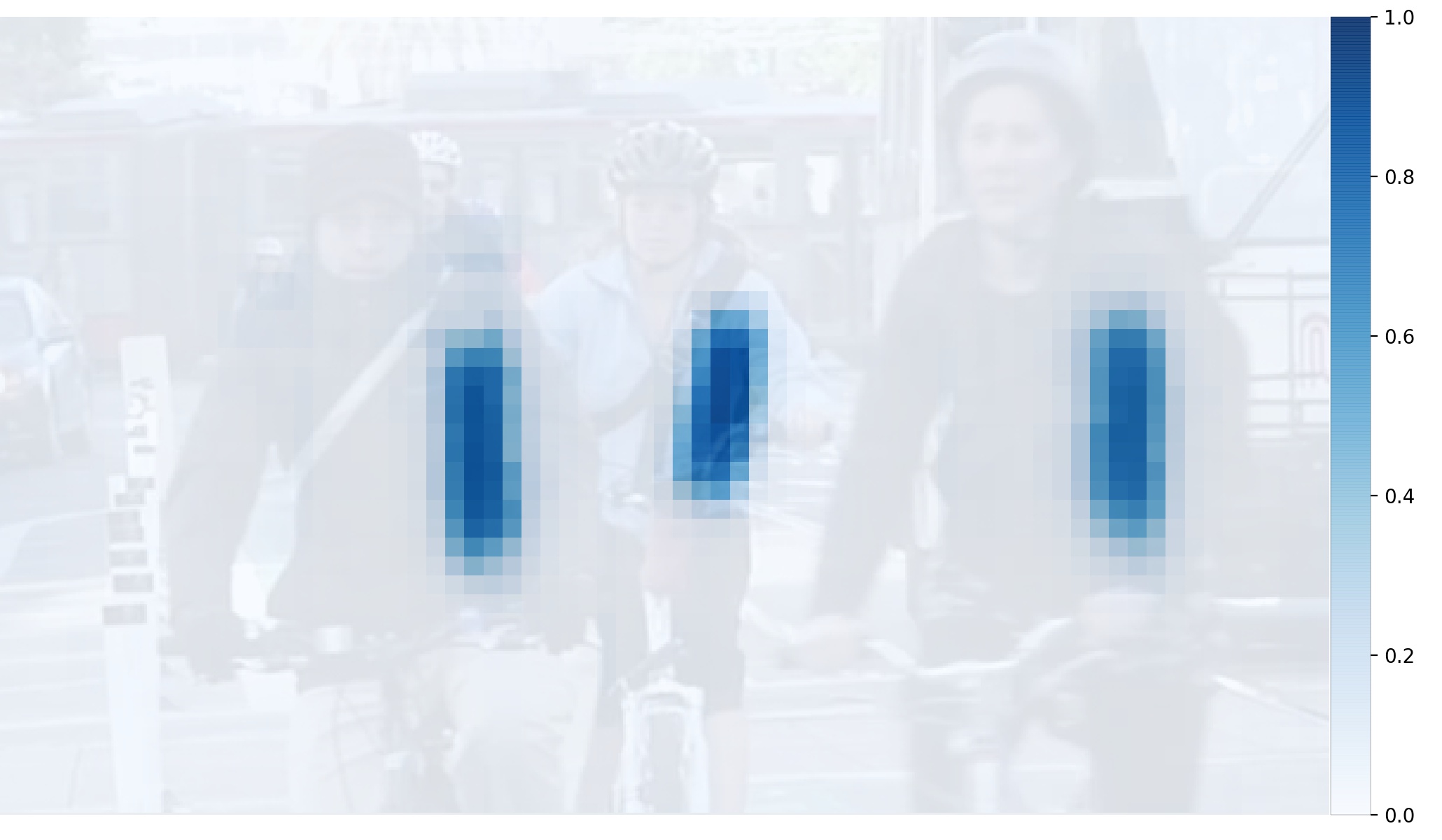
(a)

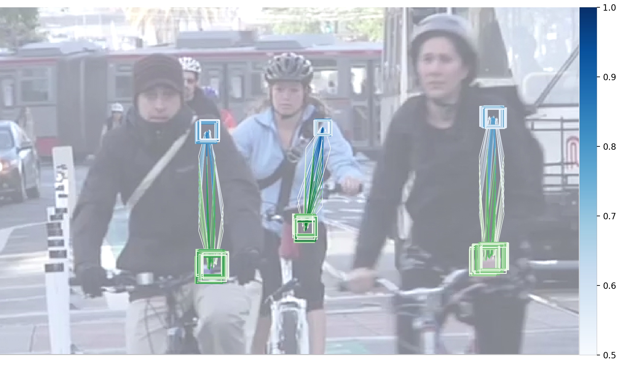
(b)

Figure 3: Visualizing the components of the CAF that associates left shoulder with left hip. This is one of the 18 CAF. Every location of the feature map is the origin of two vectors which point to the shoulders and hips to associate. The confidence of associations $\textbf{a}_{c}$ is shown at their origin in (3a) and the vector components for $\textbf{a}_{c}$ greater than 0.5 are shown in (3b).

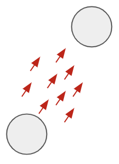
(a)

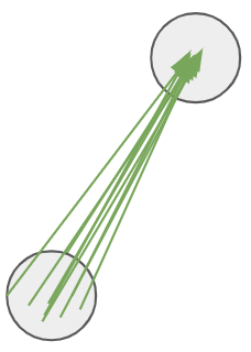
(b)

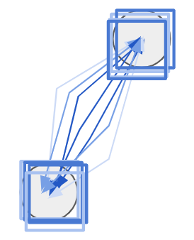
(c)

Figure 4: Common association fields between two joints. Joints are visualized as gray circles. Part Affinity Fields (a) as used in OpenPose [16] are unit vectors indicating a direction towards the next joint. Mid-range fields (b) as used in PersonLab [18] are vectors originating in the vicinity of a source joint and point to the target joint. Our Composite Association Field (c) regresses both source and target points and additionally predicts their joint size which are visualized with blue squares.

II-C Beyond Humans

While many state-of-the-art methods focused on human body pose detection and tracking, the research community has recently studied their performance on other classes such as animals and cars. Pose estimation research for animals and cars has to deal with additional challenges: limited labeled data [33] and large number of self-occlusions [34].

For animals, datasets are usually small and include limited animal species [35, 33, 36, 37, 38]. To overcome this issue, DeepLabCut [39] and WS-CDA [33] have developed transfer learning techniques from humans to animals. Mu et al. [40] have generated a synthetic dataset from CAD animal models and proposed a technique to bridge the real-synthetic domain gap. Another line of work has extended the human SMPL model [41] to animals to learn simultaneously pose and shape of endangered animals [42, 43, 44].

For cars, self-occlusions between keypoints are inevitable. A few methods improve performances by estimating 2D and 3D keypoints of vehicles together. Occlusion-net [34] uses a 3D graph network with self-supervision to predict 2D and 3D keypoints of vehicles using the CarFusion dataset [45], while GSNet [46] predicts 6DoF car pose and reconstructs dense 3D shape simultaneously. Without 3D information, the popular OpenPose [47] shows qualitative results for vehicles and Simple Baseline [48] extends a top-down pose estimator for cars on a custom dataset based on Pascal3D+ [49].

III Composite Fields

Our method relies on the Composite Fields formalism to jointly detect and track semantic keypoints. Hereafter, we briefly present them.

Field Notation

Fields are functions over locations (e.g., feature map cells) and their outputs are primitives like scalars or composites. Composite Fields as introduced in [11] jointly predict multiple variables of interest, for example, the confidence, precise location and size of a semantic keypoint (e.g., body joint).

We will enumerate the spatial output coordinates of the neural network with $i,j$ and reserve $x,y$ for real-valued coordinates in the input image. A field over $(i,j)$ is denoted with $\textbf{f}^{ij}$ and can have scalar, vector or composite values. For example, the composite field of scalars $s$ and 2D vector components $v_{x},v_{y}$ is $\{s,v_{x},v_{y}\}^{ij}$. This is equivalent to “overlaying” a confidence map with a vector field if the ground truth is aligned. This equivalence is trivial in this example but becomes more subtle when we discuss association fields below.

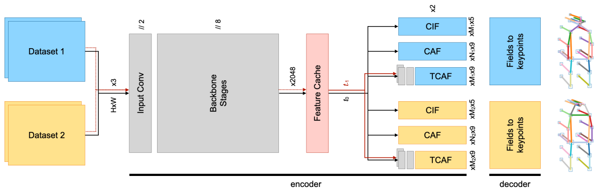
Figure 5: Model architecture. The input is an image batch of size $(H,W)$ with three color channels, indicated by “x3”. During joint training on multiple datasets, the datasets produce image pairs (black arrows for current image at $t_{0}$ and red arrows for image at $t_{-1}$) whereas during evaluation they produce single images in a sequence. The neural network based encoder produces composite fields for $M$ joints and $N$ connections. An operation with stride two is indicated by “//2”. The shared backbone is a ResNet [50] or ShuffleNetV2 [51] without max-pooling. The Feature Cache is only used during evaluation and injects for every image the previous feature map into the batch. We use a single $1\times 1$ convolution in each head network. The TCAF head networks have a shared pre-processing step consisting of a feature reduction to 512 with a $1\times 1$ convolution followed by ReLU, a concatenation of the two feature maps and another $1\times 1$ convolution with ReLU activation. For optional spatial upsampling, we append a sub-pixel convolution layer [52] to each head network. The decoder converts a set of composite fields into pose estimates. Each semantic keypoint is represented by a confidence score, a real-valued ($x$, $y$) coordinate pair and a size estimate.

Composite Intensity Fields (CIF)

The Composite Intensity Fields (CIF) characterize the intensity of semantic keypoints. The composite structure is based on [53] with the extension of a scale $\sigma$ to characterize the keypoint size. This is identical to the part intensity field in [11]. We use the notation $\textbf{p}^{ij}_{J}=\{c,x,y,b,\sigma\}^{ij}_{J}$ where $J$ is a particular body joint type, $c$ is the confidence, $x$ and $y$ are regressed coordinates, $b$ is the uncertainty in the location and $\sigma$ is the size of the joint.

Figure 2 shows the components of a CIF field and a high resolution accumulation of the predicted intensity. The field is coarse with a stride of 16 with respect to the input image but the accumulated intensity is at high resolution. The high resolution confidence map $f(v,w)$ is a convolution of an unnormalized Gaussian kernel $\mathcal{N}$ with width $\sigma$ over the regressed targets from the Composite Intensity Field $x$ and $y$ weighted by its confidence $c$:

$$f_{J}(v,w)=\sum_{ij}c^{ij}_{J}\;\mathcal{N}(v,w|x^{ij}_{J},y^{ij}_{J},\sigma^{ij}_{J})$$ (1)

where $v$ and $w$ are real-valued coordinates in the image. This accumulation incorporates information of the confidence $c$, the precisely regressed spatial location $(x,y)$ and the predicted joint size $\sigma$. This map $f_{J}$ is used to seed the pose decoder and to rescore predicted CAF associations.

Composite Association Fields (CAF)

Efficiently forming associations is the core challenge for tracking multiple poses in a video sequence. The most difficult cases are crowded scenes and camera angles where people occlude other people – as is the case in the self-driving car perspective where pedestrians occlude other pedestrians. Top-down methods first estimate bounding boxes and then do single-person pose estimation per bounding box. This assumes non-overlapping bounding boxes which is not given in our scenario. Therefore, we focus on bottom-up methods.

In [11], we introduced Part Association Fields to connect joint locations together into poses. Here, we extend this field with joint-scale components and call it Composite Association Field (CAF) to distinguish it better from Part Affinity Fields introduced in [16]. A graphical review of association fields is shown in Figure 4 and shows that our CAF expresses the most detail about an association.

CAFs predict a confidence, two vectors to the two parts this association is connecting, two spreads $b$ for the spatial precisions of the regressions (details in Section IV-A) and two joint sizes $\sigma$. CAFs are represented with $\textbf{a}^{ij}_{J_{1}\leftrightarrow J_{2}}=\{c,x_{1},y_{1},x_{2},y_{2},b_{1},b_{2},\sigma_{1},\sigma_{2}\}^{ij}_{J_{1}\leftrightarrow J_{2}}$ where $J_{1}\leftrightarrow J_{2}$ is the association between body joints $J_{1}$ and $J_{2}$. Predicted associations between left shoulders and left hips are shown for an example image in Figure 3. In our representation of an association, physically meaningful quantities are regressed to continuous variables and do not suffer from the discreteness of the feature map. In addition, it is important to represent associations between two joints that are at the same pixel location. Our representation is stable for these zero-distance associations – something that Part Affinity Fields [16] cannot do – which becomes particularly important when we introduce our extension for tracking.

IV Method

We aim to present a method that can detect, associate and track semantic keypoints in videos efficiently. We place particular emphasis on urban and crowded scenes that are difficult for autonomous vehicles. Many previous methods struggle when object bounding boxes overlap. In bird-eye views from drones or security cameras, bounding boxes are more separated than in a car driver’s perspective. Here, top-down methods struggle. Previous bottom-up methods have been trailing top down methods in accuracy without improving on performance either. Our bottom-up method is efficient, employs a stable field representation and has high accuracy and performance that even surpasses top-down methods.

Figure 5 presents our model architecture. It is a shared ResNet [50] or ShuffleNetV2 [51] base network without max-pooling. The head networks are shallow and not shared between datasets. In our examples, each dataset has a head network for joint intensities (Composite Intensity Field – CIF) and a head network for associations (Composite Association Field – CAF). Beyond CIF and CAF, additional head networks can be added. In Section IV-B, we introduce the new Temporal Composite Association Field (TCAF) which is predicted by an additional head network to facilitate pose tracking.

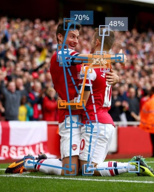
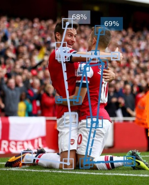
Figure 6: Effect of self-hidden keypoint suppression during training. The left image is without and the right image is with self-hidden keypoint suppression. The left hips of both soccer players collide in pixel space.

We will introduce a tracking method that is a direct extension of single-image pose estimation. Therefore, we first introduce our method for single-image pose estimation with particular emphasis on details that will be relevant for pose tracking.

IV-A Single-Image Pose Estimation

Loss Functions for Composite Fields

Human pose estimation algorithms tend to struggle with the diversity of scales that a human pose can have in an image. While a localization error for the joint of a large person can be minor, that same absolute error might be a major mistake for a small person. Our loss is the logarithm of the probability that all components are “well” predicted, i.e., it is the sum of the log-probabilities for the individual components. Each component follows standard loss prescriptions. We use binary cross entropy (BCE) for classification with a Focal loss modification $w$ [54]. To regress locations in the image, we use the Laplace loss [55] which is an $L_{1}$-type loss that is attenuated by a predicted spread $\hat{b}$ in the location. To regress additional scale components (keypoint sizes), we use a Laplace loss with a fixed spread $b_{\sigma}$ = 3. The CIF loss function is:

$$\mathcal{L}_{\textrm{CIF}} = \sum\limits_{m_{c}}w(c,\hat{c})\textrm{BCE}(c,\hat{c})$$ (4)

$$+\;\;\sum\limits_{m_{v}}\frac{1}{\hat{b}}L_{2}(v,\hat{v},b_{\textrm{min}})+\log\hat{b}$$

$$+\;\;\sum\limits_{m_{s}}\frac{1}{b_{s}}\left|1-\frac{\hat{s}}{s}\right|$$

with its three parts for confidence (4), localization (4) and scale (4) and where:

$$L_{2}(v,\hat{v},b_{\textrm{min}})=\sqrt{(v_{1}-\hat{v}_{1})^{2}+(v_{2}-\hat{v}_{2})^{2}+b_{\textrm{min}}^{2}}\;\;\;.$$ (5)

The sums are over masked feature cells $m_{c}$, $m_{v}$ and $m_{\sigma}$ with $i,j,J$ implied. The mask for confidence $m_{c}$ is almost the entire image apart from regions annotated as “crowd regions” [2]. The masks for localization $m_{v}$ and for scale $m_{\sigma}$ are only active in a $4\times 4$ window around the ground truth keypoint. Per feature map cell, there is a ground truth confidence $c$ and its predicted counterpart $\hat{c}$. The predicted location $\hat{v}=(\hat{v}_{1},\hat{v}_{2})$ is optimized with a Laplace loss with a predicted spread $\hat{b}$ for heteroscedastic aleatoric uncertainty [55] with respect to the ground truth location $v$. A $b_{\textrm{min}}=1\textrm{px}$ is added to prevent exploding losses when the spread becomes too small. For stability, we clip the BCE loss when it becomes larger than five. The CAF loss has the same structure but with two localization components (4) and two scale components (4).

Self-Hidden Keypoint Suppression

The COCO evaluation metric treats visible and hidden keypoints in the same manner. As in [11], we include hidden keypoints in our training. However, when a visible and a hidden keypoint appear close together, we remove the hidden keypoint from the ground truth annotation so that this keypoint is not included in associations. In Figure 6, we show the effect of excluding these self-hidden keypoints from training and observe better pose reconstruction when a keypoint hides another keypoint of the same type.

Greedy Decoder with Frontier

The composite fields are converted into sets of pose estimates with the greedy decoder introduced in [11] and reviewed here. The CIF field and its high-resolution accumulation $f(x,y)$ defined in equation 1 provide seed locations. Previously, new associations were formed starting at the joint that has currently the highest score without taking the CAF confidence of the association into account. Here, we introduce a frontier which is a priority queue of possible next associations. The frontier is ordered by the possible future joint scores which are a function of the previous joint score and the best CAF association:

$$\max_{ij}s(\textbf{a}^{ij}_{J_{1}\leftrightarrow J_{2}},\vec{x})=c\exp\left(-\frac{||\vec{x}-(x_{1},y_{1})||_{2}}{\sigma_{1}}\right)f_{J_{2}}(x_{2},y_{2})$$ (6)

where $\vec{x}$ is the source joint location, $\textbf{a}^{ij}_{J_{1}\leftrightarrow J_{2}}=(c,x_{1},y_{1},x_{2},y_{2},\sigma_{1},\sigma_{2})$ is the CAF field with implied sub-/superscripts on the components and $f_{J_{2}}$ is the high resolution confidence map of the target joint $J_{2}$. An association is rejected when it fails reverse matching. To reduce jitter, we not only use the best CAF association in the above equation but a weighted mixture of the best two associations; similar to blended connections in [56]. Only when all possible associations are added to the frontier, the connection is made to the highest priority in the frontier. This algorithm is fast and greedy. Once a connection to a new joint has been made, this decision is final.

Instance Score and Non-Maximum Suppression (NMS)

Once all poses are reconstructed, we apply NMS. Poses are first sorted by their instance score which is the weighted mean of the keypoint scores where the three highest keypoint scores are weighted three times higher. We run NMS at the keypoint level as in [11, 18]. The suppression radius is dynamic and based on the predicted joint size. We do not refine predictions.

Denser Pose Skeletons

Figure 7 gives an overview of the pose skeletons that are used in this paper. In particular, Figure 7b shows a modification of the standard COCO pose [2] with additional associations. These denser associations are redundancies in case of occlusions. The additional associations are longer-range and therefore harder to predict. The frontier in our greedy decoder takes this difficulty into account and automatically prefers easier, confident associations when available. Qualitatively, the advantage of dense associations is shown in Figure 8. With the standard COCO skeleton, the single person’s pose skeleton would be divided into two disconnected parts (left image) as indicated by the two white bounding boxes. With the additional denser associations, a single pose is formed (right image).

IV-B Pose Tracking

In the previous section we introduced our method for bottom-up pose estimation in single images. We now generalize that method to tracking poses in videos with associations between images in the same bottom-up fashion. Our unified approach forms both spatial and temporal associations simultaneously. This even leads to improved single-image poses from the additional temporal information.

Temporal Composite Association Field (TCAF)

During training, tracking data is fed into the base network as image pairs that are concatenated in the batch dimension, i.e., a batched input tensor of eight image pairs has the same shape as 16 individual images.

During prediction, the backbone processes one image at a time and each image only once. The resulting feature map is then concatenated with the previous feature map from the “Feature Cache” (see Figure 5). While there is still duplicate computation in the head networks, their computational complexity is small.

To form associations in image sequences, we introduce the Temporal Composite Association Field (TCAF). Its output structure is identical to a CAF field, but its input is based on pairs of feature maps that were created independently. To jointly process information from both feature maps, the TCAF head contains a preprocessing step of a $1\times 1$ input convolution to reduce the feature size to 512 with ReLU non-linearity, a concatenation of these two feature maps to 1024 features, a $1\times 1$ convolution with ReLU to process the two images jointly and a final $1\times 1$ convolution to produce all components necessary for a composite association field.

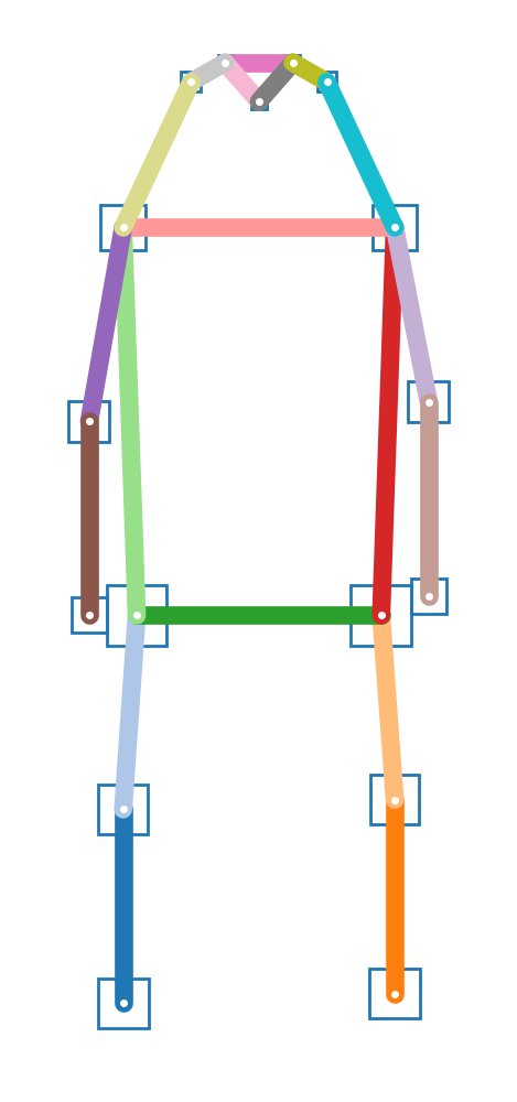
(a)

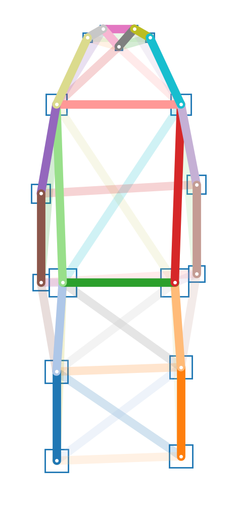
(b)

(c)

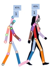
(d)

Figure 7: A COCO person pose [2] is shown in (a). Additional denser connections are shown in lighter colors in (b). The additional connections provide redundancies in case of occlusions. A pose skeleton as used in Posetrack with temporal connections is shown in (c). An example of a tracked pose is shown in (d). The first frame is captured with the right leg (blue) in front and the second frame one step later. For clarity, only connections that were used to decode the pose are shown and therefore only the temporal connection that is connecting the right ankle from the past frame to the current frame is visible.

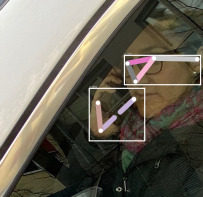
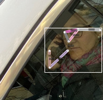
Figure 8: Left: A sparse pose cannot connect the right arm to the facial keypoints leading to the detection of two separate person instances highlighted by the two white bounding boxes. Right: An additional dense connection between the nose and right shoulder leads to a correctly identified single pose.

Spatio-Temporal Poses

Figure 7c shows a schematic of a person pose (17 joints and 18 associations) with additional temporal connections to all joints of the same kind in the previous frame. In our method, this is treated as a single pose with $2\times 17$ joints (CIF) and 18 associations (CAF) within the same frame and an additional 17 associations (TCAF) between frames.

From Spatio-Temporal Poses to Tracks

Spatio-temporal poses create temporal associations in pairs of images. We now introduce our book-keeping method to go from pairs of images to image sequences. During evaluation and for a new frame $t_{0}$, the decoder creates new tracking poses from existing tracks (poses in the previous frame $t_{-1}$) or from single-image seeds in the current frame $t_{0}$. These partial poses are then completed using the same greedy frontier decoder described for single images. Once all spatio-temporal poses are complete, the $t_{0}$ joints are extracted into single-frame poses. Every single-frame pose is already tagged with an existing track-id if the spatio-temporal pose was generated from an existing track or a new track-id if the spatio-temporal pose originated from a new seed in the current frame. The single-frame poses are then filtered with soft NMS [18] and then either added to existing tracks or they become the first poses of new tracks.

Our method is bottom-up in both pose estimation and tracking and estimates temporal and spatial connections within a single stage. Most existing work – even other bottom-up tracking methods [10, 26] – employ a two stage process where, first, spatial connections are estimated and, second, temporal connections are made.

V Experiments

Self-driving cars must perceive and predict pedestrians and other traffic participants robustly. One of the most challenging scenarios are crowded places. We will first show experiments on single-image human pose estimation in CrowdPose [12] which contains particularly challenging scenarios and on the standardized and competitive COCO [2] person keypoint benchmark. Then we will show results for pose tracking in videos on the PoseTrack 2017 [9] and 2018 [13] datasets. We have conducted extensive experiments to show the benefit of a unified bottom-up pose estimation and tracking method with spatio-temporal poses. To demonstrate the universality of our approach, we apply our method also to poses of cars and poses of animals.

V-A Datasets

CrowdPose

In [12], the CrowdPose dataset is proposed. It is a selection of images from other datasets with a particular emphasis on how crowded the images are. The crowd-index of an image represents the amount of overlap between person bounding boxes. The authors place particular emphasis on a uniform distribution of the crowd-index in all data partitions. Because this dataset is a composition of other datasets and to avoid contamination, our CrowdPose models are pretrained on ImageNet [57] and then trained on CrowdPose only. The dataset comes with a split of 10,000 images for training, 2,000 for validation and 8,000 images for the test set.

COCO

The de-facto standard for person keypoint prediction is the competitive COCO keypoint task [2]. The test set is private and powers an active leaderboard via a protected challenge server. COCO contains 56,599 diverse training images with person keypoint annotations. The validation and test-dev sets contain 5,000 and 20,288 images.

ApolloCar3D

We generalize our approach to vehicle keypoints using the ApolloCar3D dataset [58], which contains 5,277 driving images at a resolution of 4K and over 60K car instances. The authors defined 66 semantic keypoints in the dataset and, for each car, they provided annotations for the visible ones. For clarity, we choose a subset of 24 semantic keypoints and show quantitative and qualitative results on this dataset.

Animal Dataset

We evaluate the performances of our algorithm on the Animal-Pose Dataset [33], which provides annotations for five categories of animals: dog, cat, cow, horse, sheep for a total of 20 keypoints. The dataset includes 5,517 instances in more than 3,000 images. The majority of these images originally belong to the VOC dataset [59].

PoseTrack 2017 and 2018

We conduct quantitative studies of our tracking performance on the PoseTrack 2017 [9] and 2018 [13] datasets. The datasets contain short video sequences of annotated and tracked human poses in diverse situations. The PoseTrack 2018 dataset contains 593 training scenes, 170 validation scenes and 375 test scenes. The test labels are private. PoseTrack 2017 is a subset of the 2018 dataset with 292 train, 50 validation and 208 test scenes. However, the 2018 leaderboard is frozen and new results are only updated for the 2017 leaderboard. Therefore, many recent methods present results on the older, smaller dataset. Here, we will report numbers for both 2017 and 2018.

V-B Evaluation

Single-Image Multi-Person Poses

Both CrowdPose and COCO follow COCO’s keypoint evaluation method. The object keypoint similarity (OKS) score [2] is used to assign a bounding box to each keypoint as a function of the person instance bounding box area. Similar to detection, the metric computes overlaps between ground truth and predicted bounding boxes to compute the standard detection metrics average precision (AP) and average recall (AR).

CrowdPose breaks down the test set at the image level into easy, medium and hard. The easy set contains images with a crowd index in $[0,0.1]$, the medium set in $[0.1,0.8]$ and the hard set in $[0.8,1.0]$. Given the uniform crowd-index distribution, most images of the test set are in the medium category.

COCO breaks down the precision scores at the instance level for medium instances with a bounding box area of (32 px)² to (96 px)² and for large instances with a bounding box area larger than (96 px)². For each image, pose estimators have to provide the 17 keypoint locations per pose and a total score for each pose. Only the top 20 scoring poses per image are considered for evaluation.

Pose Tracks

A common metric to evaluate the tracking of human poses is the Multi Object Tracker Accuracy (MOTA) [60, 4] which is also the main metric in PoseTrack challenges and leaderboards. It combines false positives, false negatives and ID switches into a single metric. We compare against the best methods that submitted to the PoseTrack 2017 and 2018 evaluation server which computes all metrics on private test sets. These methods include strong top-down methods as well as bottom-up methods for pose estimation and tracking.

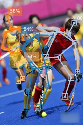
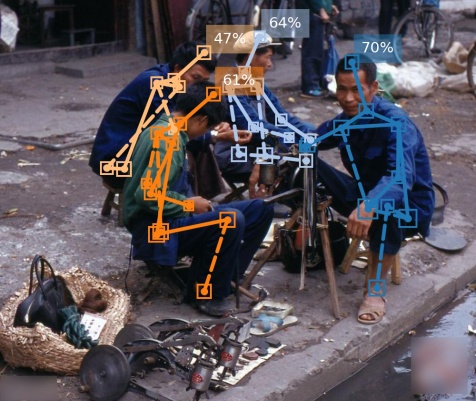
Figure 9: Illustration of OpenPifPaf predictions from the CrowdPose [12] val set with crowd-index hard on a sports scene, a family photo and a street scene.

V-C Implementation Details

Neural Network Configuration

All our models are based on ResNet [50] or ShuffleNetV2 [51] base networks and multiple head networks. The base networks have their input max-pooling operation removed as it destroys spatial information. The stride from input image to output feature map is 16 with 2048 features at each location. We apply no additional modifications to the standard ResNet models. We use the standard building blocks of ShuffleNetV2 backbones to construct our custom configurations which we denote ShuffleNetV2K16/K30. A ShuffleNetV2K16 model has the prediction accuracy of a ResNet50 with fewer parameters than a ResNet18. The configuration is specified by the number of output features of the five stages and the number of repetitions of the blocks in each stage. Our ShuffleNetV2K16 has output features (block repeats) of 24 (1), 348 (4), 696 (8), 1392 (4), 1392 (1) and our ShuffleNetV2K30 has 32 (1), 512 (8), 1024 (16), 2048 (6), 2048 (1). Spatial $3\times 3$ convolutions are replaced with $5\times 5$ convolutions which introduces only a small increase in the number of parameters because all spatial convolutions are depth-wise.

Each head network is a single $1\times 1$ convolution followed by a sub-pixel convolution [52] to double the spatial resolution bringing the total stride down to eight. Therefore, the spatial feature map size for an input image of $801\textrm{px}\times 801\textrm{px}$ is $101\times 101$. The confidence component of a field is normalized with a sigmoid non-linearity and the scale components for joint-sizes are enforced to be positive with a softplus [61].

Augmentations

We apply the standard augmentations of random horizontal flipping, random rescaling with a rescaling factor $r\in[0.5,2.0]$, random cropping and padding to $385\times 385$ followed by color jittering with 40% variation in brightness and saturation and 10% variation in hue. We also convert a random 1% of the images to grayscale and generate strong JPEG compression artifacts in 10% of the images.

The tracking task is similarly augmented. The random rescaling is adapted to an image width in $[0.5\times 801,1.5\times 801]$ and random cropping to a maximum image side of 385 px. Half of the image pairs are randomly reoriented (rotations by multiples of $90^{\circ}$). To increase the inter-frame variations, we add a small synthetic camera shift of maximum 30 px between image pairs. To further increase the variation, we form image pairs with a random interval of 4, 8 and 12 frames. In 20% of image pairs, we replace one of the images with a random image to provide a higher number of negative samples for tracking.

Single-Image Training

For ResNet [50] backbones, we use ImageNet [57] pretrained models. ShuffleNetV2 [51] models are trained from random initializations. We use the SGD [62] optimizer with Nesterov momentum [63] of 0.95, batch size of 32 and weight decay of $10^{-5}$. The learning rate is exponentially warmed up for one epoch from $10^{-3}$ of its target value. At certain epochs (specified below), the learning rate is exponentially decayed over 10 epochs by a factor of 10. We employ model averaging [64, 65] to extract stable models for validation. At each optimization step, we update an exponentially weighted version of the model parameters with a decay constant of $10^{-2}$.

On CrowdPose, which is a smaller dataset than COCO, we train for 300 epochs. We set the target learning rate to $10^{-5}$ and decay at epochs 250 and 280.

On COCO, we use a target learning rate of $10^{-4}$ and decay at epoch 130 and 140. The training time for 150 epochs of a ShuffleNetV2K16 on two V100 is approximately 37 hours. We do not use any additional datasets beyond the COCO keypoint annotations.

Training for Tracking on PoseTrack

We use the ShuffleNetV2k30 backbone for all our tracking experiments. PoseTrack 2018 is a video dataset which means that despite a large number of annotations, the variation is smaller than in single-image pose datasets. Therefore, we keep single-image pose estimation on the COCO dataset [2] as an auxiliary task and train on PoseTrack and COCO simultaneously. The type of poses that are annotated in the two datasets are similar but not identical, e.g., one dataset annotates the eyes and the other does not. During training, we alternate the two tasks between batches. In one batch we feed pairs of images from the PoseTrack dataset and apply losses to the corresponding head networks and in the next batch we feed in single images from COCO and apply losses to the other head networks (see Figure 5). The COCO task is trained identical to the single-image pose estimation discussed in the previous section, but converted from single images to pairs of tracked images via synthetic shifts of up to 30px. Starting from a trained single-image pose backbone, we train on both datasets with SGD [62] with the same configuration as for single images. We alternate the dataset every batch and only do an SGD-step every two batches. We train for 50 epochs where every epoch consists of 4994 batches. The training time is 55 minutes per epoch on two V100 GPUs.

TABLE I: Evaluation on the CrowdPose test dataset [12]. Our OpenPifPaf result is based on a ResNet50 backbone with single-scale evaluation at 641px. ^∗Values extracted from CrowdPose paper [12]. ⁺Employs multi-scale testing.

	AP	AP0.50	AP0.75	AP${}_{\textrm{easy}}$	AP${}_{\textrm{medium}}$	AP${}_{\textrm{hard}}$	FPS
Mask R-CNN∗ [15]	57.2	83.5	60.3	69.4	57.9	45.8	2.9
AlphaPose∗ [66]	61.0	81.3	66.0	71.2	61.4	51.1	10.9
HigherHRNet-W48 [24]	65.9	86.4	70.6	73.3	66.5	57.9	-
SPPE [12]	66.0	84.2	71.5	75.5	66.3	57.4	10.1
HigherHRNet-W48+ [24]	67.6	87.4	72.6	75.8	68.1	58.9	-
OpenPifPaf (ours)	70.5	89.1	76.1	78.4	72.1	63.8	13.7

V-D Results

Crowded Single-Image Pose Estimation

In Figure 9, we show example pose predictions from the CrowdPose [12] validation set. We show results in a diverse selection of sports disciplines and everyday settings. All shown images are from the hard subset with a crowd-index larger than 0.8.

In Table I, we show a quantitative comparison of our performance with other methods. We are not only more precise across all precision metrics AP, AP^0.50, AP^0.75, AP${}_{\textrm{easy}}$, AP${}_{\textrm{medium}}$ and AP${}_{\textrm{hard}}$ but also predict faster than all previous top-performing methods at 13.7 FPS (frames-per-second) on a single GTX1080Ti.

TABLE II: Evaluation metrics for the COCO 2017 test-dev dataset for bottom-up methods. Numbers are extracted from the respective papers. Our prediction time is determined on a single V100 GPU. ^∗Only evaluating images with three person instances.

	AP	APM	APL	$t$ [ms]
OpenPose [16]	61.8	57.1	68.2	100
Assoc. Emb. [17]	65.5	60.6	72.6	166
PersonLab [18]	68.7	64.1	75.5	-
MultiPoseNet [23]	69.6	65.0	76.3	43∗
HigherHRNet [24]	70.5	66.6	75.8	$>$1000
OpenPifPaf (ours)	71.9	68.5	77.4	69

COCO

All state-of-the-art methods compare their performance on the well-established COCO keypoint task [2]. Our quantitative results on the private 2017 test-dev set are shown in Table II along with other bottom-up methods. This comparison includes field-based methods [16, 18, 11] and methods based on associative embedding [17, 24]. We perform on par with the best existing bottom-up method. We evaluate on rescaled images where the longer edge is 801 px which is the same image size that will be used for tracking below. We evaluate a single forward pass without horizontal flipping and without multi-scale evaluation because we aim for a fast method. The average time per image with a GTX1080Ti is 152 ms (63 ms on a V100) of which 29 ms is used for decoding.

Pose Tracking

TABLE III: Evaluation metrics on the test sets of (a) PoseTrack 2018 [13] and (b) PoseTrack 2017 [9]. Numbers are extracted from the respective papers and the leaderboard. All methods are online methods apart from DetTrack [67].

PoseTrack 2018	MOTA	FPS		AP
openSVAI [28]	54.5	-		63.1
MIPAL [26]	54.9	-		67.8
Miracle [30]	57.4	-		70.9
MSRA/FlowTrack [19]	61.4	0.7		74.0
OpenPifPaf (ours)	61.7	12.2		71.9

(a)

PoseTrack 2017	MOTA	FPS		AP
STAF [27]	53.8	3		70.3
MIPAL [26]	54.5	-		68.8
MSRA/FlowTrack [19]	57.8	0.7		74.6
HRNet [20]	57.9	-		74.9
LightTrack [29]	58.0	-		66.6
OpenPifPaf (ours)	60.6	12.2		71.5
KeyTrack [32]	61.2	1.0		74.0
DetTrack (offline) [67]	64.1	-		74.1

(b)

We want to track multiple human poses in videos. We train and validate on the PoseTrack 2018 dataset [13]. Table III shows our main results for pose tracking on both of the private test sets of Posetrack 2017 and 2018. We also show our single-image average precision (AP) which highlights that our performant tracking method can compensate for a lower AP, e.g., compared to MSRA/FlowTrack [19], and still outperform in overall MOTA and FPS. All our results are produced in a single pass and online (without future frames). The frames per second (FPS) stated in Table III refer to the single process, sequential evaluation. In addition, we provide extra metrics that are not published on the leaderboards. For PoseTrack 2017, our MOTP is 84.5, precision is 84.1 and recall is 77.7. For PoseTrack 2018, our MOTP is 84.9, precision is 84.4 and recall is 78.3.

Spatio-temporal poses on real-world examples are shown in Figure 10. They show challenging scenarios with occlusions. Figure 11 highlights the ability of spatio-temporal poses to complete poses through time, i.e., even when a pose is partitioned because of occlusion in the current frame, multiple temporal connections (TCAF) form a single tracked pose. Similarly, for the poses 3, 4, 5 and 7 in Figure 12, the associations from shoulders to hips are often difficult because of the lighting condition. Depending on the predicted association confidences, the decoder determines automatically whether to connect to a keypoint with a spatial or temporal connection. In these difficult scenarios, the greedy decoder completed these poses with multiple temporal connections (TCAF).

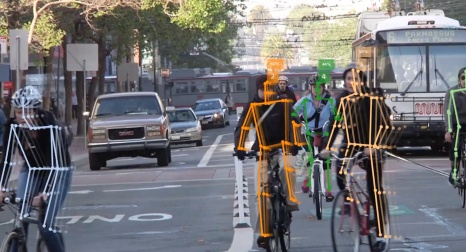
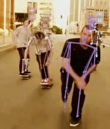
Figure 10: Qualitative results from the Posetrack 2018 [13] validation set. Images show tracks of spatio-temporal poses including their frame-to-frame associations where only connections that were used to construct the poses are shown.

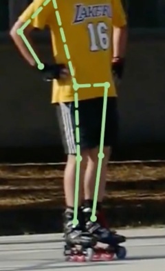
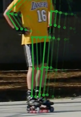
Figure 11: Qualitative results from the Posetrack 2018 [13] validation set. Left: Single-image detection. The person’s left shoulder is not visible and therefore the left arm cannot be connected to the rest of the body. Right: Spatio-temporal pose. Multiple temporal connections allow to safely connect both left and right arm to the rest of the body.

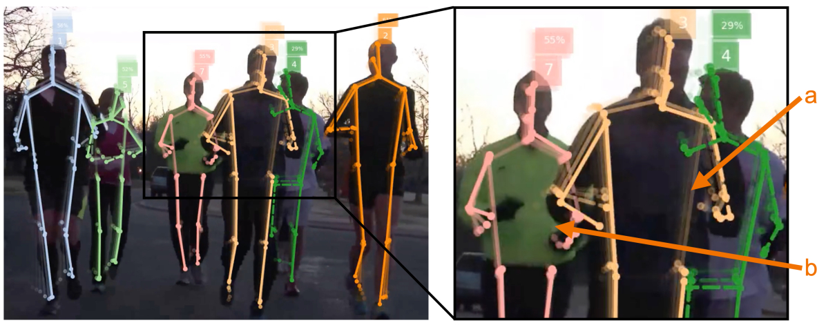
Figure 12: Qualitative results from the Posetrack 2018 [13] validation set. (a) indicates a connection that has been made spatially in a previous frame but for the last few frames the left leg of person 3 is connected to the rest of the body only through temporal connections. (b) shows a connection that is temporarily occluded by the arm of the person in front and also here our algorithm decided to connect the left leg via temporal connections instead of spatial ones.

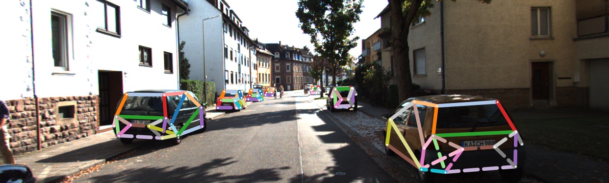
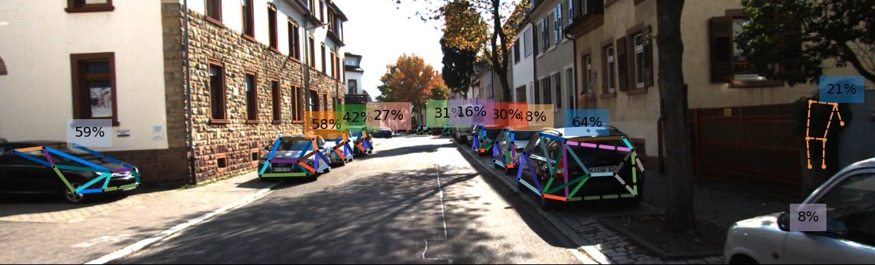
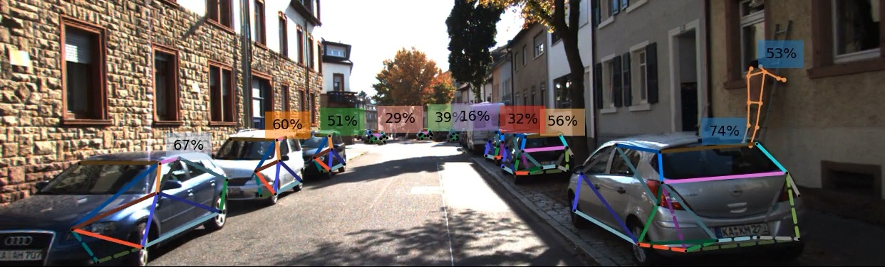
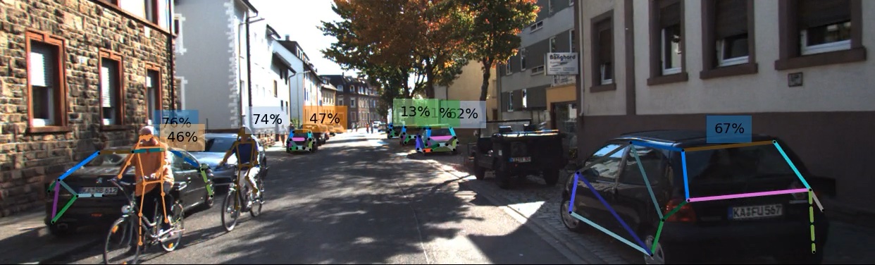
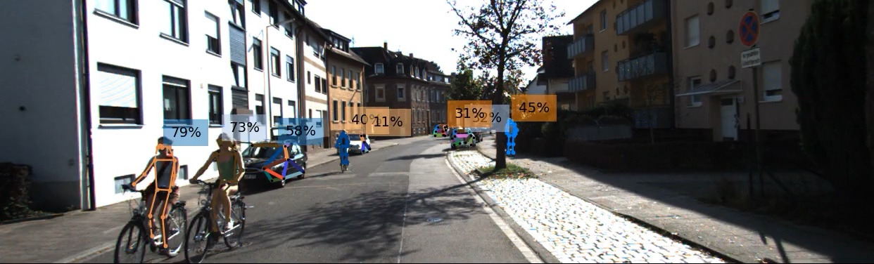
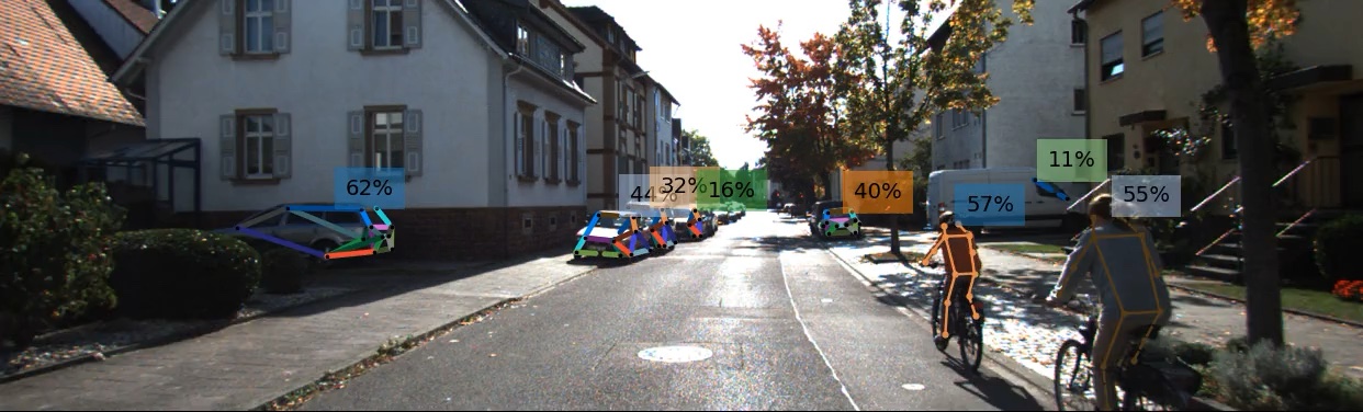
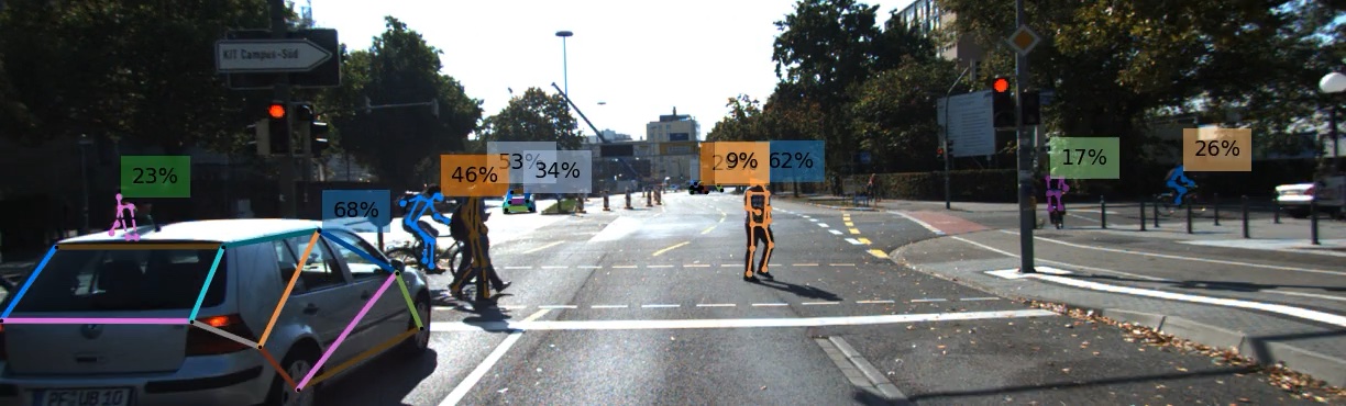
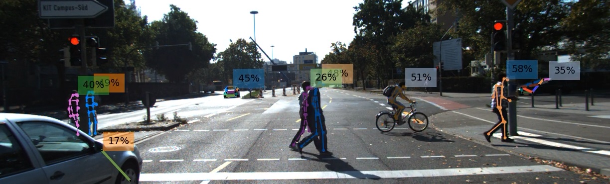
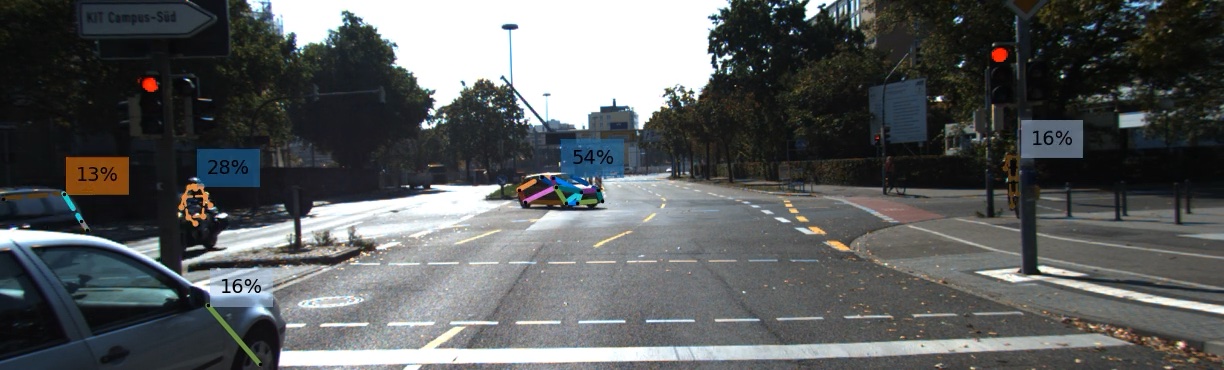
Figure 13: Qualitative results from the KITTI [68] and ApolloCar3D [58] datasets. We resolve distant pedestrians, cyclists and cars and handle changing lighting conditions well.

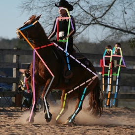
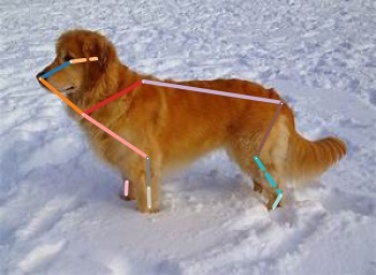
Figure 14: Qualitative results from the Animal-Pose dataset [33]. The left image was processed by a person model and an animal model.

TABLE IV: Quantifying detection performance for pedestrians, cars and animals. In the “Pedestrians” column, we show the detection rate on KITTI [68] with IoU=0.3 and instance threshold of 0.2 for all methods. For “Vehicles”, we show the keypoint detection rate on ApolloCar3D [58] which was published in previous methods and we also provide AP in the text. In the “Animals” column, we provide keypoint AP as defined in the Animal-Pose dataset [33].

Method	Pedestrians	Vehicles	Animals
Mono3D [69]	73.2	-	-
3DOP (stereo) [70]	73.1	-	-
MonoDIS [71]	60.5	-	-
SMOKE [72]	39.1	-	-
MonoPSR [73]	82.8	-	-
CPM [21]	-	75.4	-
WS-CDA [33]	-	-	44.3
OpenPifPaf (ours)	84.6	86.1	47.8
Human labelers [58]	-	92.4	-

Pedestrian, Car and Animal Poses

A holistic perception framework for autonomous vehicles also needs to be able to generalize to other classes than humans. We show that we can predict poses of cars and animals with high accuracy in Figures 13 and 14 and provide a quantitative summary in Table IV.

On car instances, our model achieves an average precision (AP) of 76.1%. The AP metric follows the same protocol of human instances, but to the best of our knowledge no previous method has evaluated AP on ApolloCar3D [58] without leveraging 3D information. Hence, we include a study on the keypoint detection rate, which has been defined in the ApolloCar3D dataset [58] and considers a keypoint to be correctly estimated if the error is less than 10 pixels. Our method achieves a detection rate of 86.1% compared to 75.4% of CPM [21]. Notably, the authors of ApolloCar3D [58] also report the detection rate of the human labelers to be 92.4%.

On animal instances, our model achieves an AP of 47.8%, compared to 44.3% of WS-CDA, the baseline developed by the authors of the Animal-Pose dataset [33]. Lower performances on animals are due to the smaller dataset size with just 4K training instances. Simultaneous training for humans and animals to achieve better generalization is left for future work.

V-E Ablation Studies

TABLE V: Ablation studies of skeleton choice and decoder configurations for single-image pose estimation. All results (except where explicitly stated otherwise) are produced with the same ShuffleNetV2k16 model on the COCO val set [2] on a single GTX1080Ti. First, we review different backbone architectures (a ResNet50 [50] and a larger ShuffleNetV2 [51]). Second, we show that only using confident keypoints leads to a large drop in precision. Third, we observe that the Frontier decoder is more important for denser skeletons while incurring almost no overhead on sparse skeletons. Fourth, we can produce a memory-efficient version of our decoder at a cost of 1.4% in AP. The biggest drop in accuracy comes from not rescoring the CAF field and the largest contributor to increasing the inference time is not rescoring the seeds.

			AP	AP0.50	AP0.75	APM	APL	$t$ [ms]	$t_{\textrm{dec}}$ [ms]
	original (ShuffleNetV2K16)		66.8	86.5	73.2	62.1	74.6	50	19
Backbone	ResNet50		68.2	87.9	74.6	65.8	72.7	64	22
	ShuffleNetV2K30		71.0	88.8	77.7	66.6	78.5	92	16
Keypoints	independent-only		-8.1	-6.3	-9.5	-8.7	-7.3	$\pm 0$	$\pm 0$
Frontier decoder	no-frontier		$\pm 0.0$	-0.1	+0.1	$\pm 0.0$	-0.1	-1	-1
	dense		+0.1	+0.2	+0.2	-0.3	+0.5	+15	+15
	no-frontier and dense		-0.3	+0.1	-0.1	-0.5	$\pm 0.0$	+14	+14
memory efficient	no seed rescoring		-0.1	-0.4	-0.1	+0.2	+0.1	+71	+54
	no seed rescoring (with NMS)		+0.1	+0.1	$\pm 0.0$	+0.2	+0.0	+19	+15
	no CAF rescoring		-1.0	-0.3	-1.0	-1.0	-1.7	-1	-1
	no rescoring (with NMS), without HR		-1.4	-0.4	-1.4	-1.0	-2.3	+9	+7

We study the impact of the backbone, the precise criteria for a keypoint, our proposed Frontier decoder, a memory efficient decoder, alternatives to TCAF and the impact of input image size. We start with studies for single images on the COCO val set (Table V) before moving to tracking studies for PoseTrack (Table VI).

Our single-image studies are run with an option to force complete poses. This is the common practice as the COCO metric does not penalize false positive keypoints within poses. This option would not be used in most real-world settings. Without forcing complete poses, the decoding time and the total prediction time is reduced by about 10ms.

Backbone

The reference backbone is a small ShuffleNetV2K16. We show comparisons to the larger ResNet50 and ShuffleNetV2K30 backbones and show how they improve precision (AP) and at what cost in timing.

Keypoint Criterium

We try to illuminate why our precision and speed is significantly better than OpenPose [16]. OpenPose first detects keypoints and then associates them. Therefore, every keypoint has to be detectable individually. In OpenPifPaf, new keypoint associations are generated from a source keypoint. These new keypoints are not previously known. They are discovered in the association. That allows OpenPifPaf to generate poses from a strong seed keypoint and connect to less confident keypoints. In “independent-only”, we restrict the keypoints of OpenPifPaf to be all of the quality of an independent seed keypoint and observe a dramatic drop of 8.1% in AP.

Frontier Decoder

Next, we study the impact of the Frontier decoder with respect to a simpler decoder without frontier. The standard pose is sparsely connected and, therefore, the frontier only has few alternatives to prioritize. For a denser pose (“dense”), the impact of the frontier (compare with “no-frontier and dense”) is more pronounced (+0.3 AP).

Memory Efficient Decoding

In the bottom part of Table V, we study the effect of removing the high-resolution accumulation map (HR) to reduce the memory footprint. This high resolution map is used in two places. First, to rescore the seeds and, second, to rescore the CAF. The impact of the seed rescoring is only 0.1 in AP but comes at a large cost in decoding time. As an alternative, we investigate a local non-maximum suppression (NMS) that selects a seed only if it is the highest confidence in a $3\times 3$ window (introduced in CenterNet [74]). This NMS reduces the decoding time but not back to the original speed. Independently, we study the impact of rescoring the CAF field which is about +1.0% in AP. Only when both the seed rescoring and the CAF rescoring are removed, the creation of the HR maps can be omitted. In that memory efficient configuration (bottom line in Table V), the AP dropped by 1.4% with respect to “original”. This demonstrates the importance of the high-resolution accumulation for speed and accuracy and which should only be removed when absolutely necessary.

TABLE VI: Baselines and ablation studies on the PoseTrack 2018 validation set [13] on a single V100 GPU. We outperform Hungarian trackers with euclidean and OKS distance functions in accuracy for a small overhead in FPS. We also study our sensitivity to the input image size. For image sizes of 513px, we observe a drop of 2.9 in MOTA but run 82% faster at 22.2 FPS.

		MOTA		FPS
	original (801px)	66.4		12.2
Hungarian	euclidean	-1.5		+4%
	OKS	-2.0		+1%
Image size	513px	-2.9		+82%
	641px	-0.9		+37%
	1201px	-1.7		-49%

Tracking Baselines

We conducted detailed studies of our method on the Posetrack 2018 validation set that are shown in Table VI. First, we created two baselines ourselves. Both baselines first do single-image pose estimation and then use the Hungarian algorithm [75] to track poses from frame to frame. Our first algorithm uses a simple Euclidean distance between joints to construct a pose similarity score. Our second method replaces the Euclidean distance with an OKS-based distance that is used in the COCO metric to compare predictions to ground truth. Both methods show a drop in MOTA of 1.5 and 2.0 while operating at about the same speed as our “original” model. This demonstrates that the overhead of our tracking network is comparable to the small overhead of the Hungarian algorithm with respect to the single-image model.

Tracking Ablation

We studied the effect of input image size at the bottom of Table VI. Our “original” model rescales the image width to 801px. Larger images do not show an improvement in accuracy (MOTA) while becoming significantly slower. Smaller input images decrease MOTA but at the same time can drastically increase speed. Most applications can probably tolerate an accuracy reduction by 0.9 in MOTA to improve speed by +37%. When the input image size is reduced to 513px, MOTA drops by 2.9 (still a great result) which comes with a speed improvement of +82% to a fast 22.2 FPS.

VI Conclusions

We have demonstrated a new method for bottom-up pose tracking for 2D human poses and shown its strength in crowded and occluded scenes that are relevant for perception in self-driving cars and social robots. We outperform previous state-of-the-art methods on CrowdPose and on PoseTrack2018. On PoseTrack2017 we are on par with the state-of-the-art but run an order of magnitude faster. We have also shown that our method generalizes to pose estimation of cars and animals. We can run all versions simultaneously on an image sequence and form the union of the predictions. In the future, we can investigate shared backbone architectures to create a holistic perception framework for autonomous vehicles.

VII Acknowledgements

This work was supported by the Swiss National Science Foundation under the Grant 2OOO21-L92326 and the SNSF Spark fund (190677). We also thank our lab members and reviewers for their valuable comments.

Sven Kreiss is a postdoc at the Visual Intelligence for Transportation (VITA) lab at EPFL in Switzerland focusing on perception with composite fields. Before returning to academia, he was the Senior Data Scientist at Sidewalk Labs (Alphabet, Google sister) and worked on geospatial machine learning for urban environments. Prior to his industry experience, Sven developed statistical tools and methods used in particle physics research.

Lorenzo Bertoni is a doctoral student at the Visual Intelligence for Transportation (VITA) lab at EPFL in Switzerland focusing on 3D vision for vulnerable road users. Before joining EPFL, Lorenzo was a management consultant at Oliver Wyman and a visiting researcher at the University of California, Berkeley, working on predictive control of autonomous vehicles. Lorenzo received Bachelors and Masters Degrees in Engineering from the Polytechnic University of Turin and the University of Illinois at Chicago.

Alexandre Alahi is an Assistant Professor at EPFL. He spent five years at Stanford University as a Post-doc and Research Scientist after obtaining his Ph.D. from EPFL. His research enables machines to perceive the world and make decisions in the context of transportation problems and smart environments. He has worked on the theoretical challenges and practical applications of socially-aware Artificial Intelligence, i.e., systems equipped with perception and social intelligence. He was awarded the Swiss NSF early and advanced researcher grants for his work on predicting human social behavior. Alexandre has also co-founded multiple startups such as Visiosafe, and won several startup competitions. He was elected as one of the Top 20 Swiss Venture leaders in 2010.

References

- [1] M. Andriluka, L. Pishchulin, P. Gehler, and B. Schiele, “2d human pose estimation: New benchmark and state of the art analysis,” in IEEE Conference on Computer Vision and Pattern Recognition (CVPR), June 2014.
- [2] T.-Y. Lin, M. Maire, S. Belongie, J. Hays, P. Perona, D. Ramanan, P. Dollár, and C. L. Zitnick, “Microsoft coco: Common objects in context,” in European Conference on Computer Vision (ECCV). Springer, 2014, pp. 740–755.
- [3] A. Crow, “How safe are self-driving cars?” Rocky Mountain Institute, 5 2017. [Online]. Available: https://rmi.org/safe-self-driving-cars/
- [4] A. Milan, L. Leal-Taixé, I. Reid, S. Roth, and K. Schindler, “Mot16: A benchmark for multi-object tracking,” arXiv preprint arXiv:1603.00831, 2016.
- [5] M. Kristan, J. Matas, A. Leonardis, M. Felsberg, L. Cehovin, G. Fernandez, T. Vojir, G. Hager, G. Nebehay, and R. Pflugfelder, “The visual object tracking vot2015 challenge results,” in Proceedings of the IEEE international conference on computer vision workshops, 2015, pp. 1–23.
- [6] M. Kristan, A. Leonardis, J. Matas, M. Felsberg, R. Pflugfelder, L. Cehovin Zajc, T. Vojir, G. Hager, A. Lukezic, A. Eldesokey et al., “The visual object tracking vot2017 challenge results,” in Proceedings of the IEEE international conference on computer vision workshops, 2017, pp. 1949–1972.
- [7] B. D. Lucas, T. Kanade et al., “An iterative image registration technique with an application to stereo vision,” 1981.
- [8] E. Insafutdinov, M. Andriluka, L. Pishchulin, S. Tang, E. Levinkov, B. Andres, and B. Schiele, “Arttrack: Articulated multi-person tracking in the wild,” in Conference on Computer Vision and Pattern Recognition (CVPR), 2017, pp. 6457–6465.
- [9] U. Iqbal, A. Milan, and J. Gall, “Posetrack: Joint multi-person pose estimation and tracking,” in Conference on Computer Vision and Pattern Recognition (CVPR), 2017, pp. 2011–2020.
- [10] A. Doering, U. Iqbal, and J. Gall, “Joint flow: Temporal flow fields for multi person tracking,” arXiv preprint arXiv:1805.04596, 2018.
- [11] S. Kreiss, L. Bertoni, and A. Alahi, “Pifpaf: Composite fields for human pose estimation,” in Conference on Computer Vision and Pattern Recognition (CVPR), June 2019.
- [12] J. Li, C. Wang, H. Zhu, Y. Mao, H.-S. Fang, and C. Lu, “Crowdpose: Efficient crowded scenes pose estimation and a new benchmark,” in Proceedings of the IEEE Conference on Computer Vision and Pattern Recognition, 2019, pp. 10 863–10 872.
- [13] M. Andriluka, U. Iqbal, E. Insafutdinov, L. Pishchulin, A. Milan, J. Gall, and B. Schiele, “Posetrack: A benchmark for human pose estimation and tracking,” in Conference on Computer Vision and Pattern Recognition (CVPR), 2018, pp. 5167–5176.
- [14] A. Toshev and C. Szegedy, “Deeppose: Human pose estimation via deep neural networks,” in Conference on Computer Vision and Pattern Recognition (CVPR), 2014, pp. 1653–1660.
- [15] K. He, G. Gkioxari, P. Dollár, and R. Girshick, “Mask r-cnn,” in Computer Vision (ICCV), 2017 IEEE International Conference on. IEEE, 2017, pp. 2980–2988.
- [16] Z. Cao, T. Simon, S.-E. Wei, and Y. Sheikh, “Realtime multi-person 2d pose estimation using part affinity fields,” in Conference on Computer Vision and Pattern Recognition (CVPR), 2017, pp. 7291–7299.
- [17] A. Newell, Z. Huang, and J. Deng, “Associative embedding: End-to-end learning for joint detection and grouping,” in Advances in Neural Information Processing Systems, 2017, pp. 2277–2287.
- [18] G. Papandreou, T. Zhu, L.-C. Chen, S. Gidaris, J. Tompson, and K. Murphy, “Personlab: Person pose estimation and instance segmentation with a bottom-up, part-based, geometric embedding model,” in European Conference on Computer Vision (ECCV), 2018, pp. 269–286.
- [19] B. Xiao, H. Wu, and Y. Wei, “Simple baselines for human pose estimation and tracking,” in Proceedings of the European conference on computer vision (ECCV), 2018, pp. 466–481.
- [20] K. Sun, B. Xiao, D. Liu, and J. Wang, “Deep high-resolution representation learning for human pose estimation,” in Conference on Computer Vision and Pattern Recognition (CVPR), 2019, pp. 5693–5703.
- [21] S.-E. Wei, V. Ramakrishna, T. Kanade, and Y. Sheikh, “Convolutional pose machines,” in Conference on Computer Vision and Pattern Recognition (CVPR), 2016, pp. 4724–4732.
- [22] A. Newell, K. Yang, and J. Deng, “Stacked hourglass networks for human pose estimation,” in European Conference on Computer Vision (ECCV). Springer, 2016, pp. 483–499.
- [23] M. Kocabas, S. Karagoz, and E. Akbas, “Multiposenet: Fast multi-person pose estimation using pose residual network,” in European Conference on Computer Vision (ECCV), 2018, pp. 417–433.
- [24] B. Cheng, B. Xiao, J. Wang, H. Shi, T. S. Huang, and L. Zhang, “Higherhrnet: Scale-aware representation learning for bottom-up human pose estimation,” in Proceedings of the IEEE/CVF Conference on Computer Vision and Pattern Recognition, 2020, pp. 5386–5395.
- [25] L. Pishchulin, E. Insafutdinov, S. Tang, B. Andres, M. Andriluka, P. V. Gehler, and B. Schiele, “Deepcut: Joint subset partition and labeling for multi person pose estimation,” in Conference on Computer Vision and Pattern Recognition (CVPR), 2016, pp. 4929–4937.
- [26] J. Hwang, J. Lee, S. Park, and N. Kwak, “Pose estimator and tracker using temporal flow maps for limbs,” in 2019 International Joint Conference on Neural Networks (IJCNN). IEEE, 2019, pp. 1–8.
- [27] Y. Raaj, H. Idrees, G. Hidalgo, and Y. Sheikh, “Efficient online multi-person 2d pose tracking with recurrent spatio-temporal affinity fields,” in Conference on Computer Vision and Pattern Recognition (CVPR), 2019, pp. 4620–4628.
- [28] G. Ning, P. Liu, X. Fan, and C. Zhang, “A top-down approach to articulated human pose estimation and tracking,” in European Conference on Computer Vision (ECCV), 2018, pp. 0–0.
- [29] G. Ning, J. Pei, and H. Huang, “Lighttrack: A generic framework for online top-down human pose tracking,” in Proceedings of the IEEE/CVF Conference on Computer Vision and Pattern Recognition Workshops, 2020, pp. 1034–1035.
- [30] D. Yu, K. Su, J. Sun, and C. Wang, “Multi-person pose estimation for pose tracking with enhanced cascaded pyramid network,” in European Conference on Computer Vision (ECCV), 2018.
- [31] S. Jin, W. Liu, W. Ouyang, and C. Qian, “Multi-person articulated tracking with spatial and temporal embeddings,” in Conference on Computer Vision and Pattern Recognition (CVPR), 2019, pp. 5664–5673.
- [32] M. Snower, A. Kadav, F. Lai, and H. P. Graf, “15 keypoints is all you need,” arXiv preprint arXiv:1912.02323, 2019.
- [33] J. Cao, H. Tang, H.-S. Fang, X. Shen, C. Lu, and Y.-W. Tai, “Cross-domain adaptation for animal pose estimation,” in Proceedings of the IEEE International Conference on Computer Vision (ICCV), 2019, pp. 9498–9507.
- [34] N. D. Reddy, M. Vo, and S. G. Narasimhan, “Occlusion-net: 2d/3d occluded keypoint localization using graph networks,” in Proceedings of the IEEE Conference on Computer Vision and Pattern Recognition (CVPR), 2019, pp. 7326–7335.
- [35] T. D. Pereira, D. E. Aldarondo, L. Willmore, M. Kislin, S. S.-H. Wang, M. Murthy, and J. W. Shaevitz, “Fast animal pose estimation using deep neural networks,” Nature methods, vol. 16, no. 1, pp. 117–125, 2019.
- [36] B. Biggs, O. Boyne, J. Charles, A. Fitzgibbon, and R. Cipolla, “Who left the dogs out? 3d animal reconstruction with expectation maximization in the loop,” in European Conference on Computer Vision (ECCV). Springer, 2020, pp. 195–211.
- [37] S. Li, J. Li, H. Tang, R. Qian, and W. Lin, “Atrw: A benchmark for amur tiger re-identification in the wild,” in Proceedings of the 28th ACM International Conference on Multimedia. New York, NY, USA: Association for Computing Machinery, 2020, p. 2590–2598.
- [38] A. Mathis, M. Yüksekgönül, B. Rogers, M. Bethge, and M. W. Mathis, “Pretraining boosts out-of-domain robustness for pose estimation,” in Proceeding of the IEEE Winter Conference on Applications of Computer Vision (WACV), 2021.
- [39] A. Mathis, P. Mamidanna, K. M. Cury, T. Abe, V. N. Murthy, M. W. Mathis, and M. Bethge, “Deeplabcut: markerless pose estimation of user-defined body parts with deep learning,” Nature Publishing Group, Tech. Rep., 2018.
- [40] J. Mu, W. Qiu, G. D. Hager, and A. L. Yuille, “Learning from synthetic animals,” in Proceedings of the IEEE Conference on Computer Vision and Pattern Recognition (CVPR), 2020, pp. 12 386–12 395.
- [41] M. Loper, N. Mahmood, J. Romero, G. Pons-Moll, and M. J. Black, “Smpl: A skinned multi-person linear model,” ACM transactions on graphics (TOG), vol. 34, no. 6, pp. 1–16, 2015.
- [42] S. Zuffi, A. Kanazawa, and M. J. Black, “Lions and tigers and bears: Capturing non-rigid, 3d, articulated shape from images,” in Proceedings of the IEEE Conference on Computer Vision and Pattern Recognition (CVPR), 2018, pp. 3955–3963.
- [43] B. Biggs, T. Roddick, A. Fitzgibbon, and R. Cipolla, “Creatures great and smal: Recovering the shape and motion of animals from video,” in Asian Conference on Computer Vision (ACCV). Springer, 2018, pp. 3–19.
- [44] S. Zuffi, A. Kanazawa, T. Berger-Wolf, and M. Black, “Three-d safari: Learning to estimate zebra pose, shape, and texture from images “in the wild”,” in Proceedings of the IEEE International Conference on Computer Vision (ICCV), 2019, pp. 5358–5367.
- [45] N. Dinesh Reddy, M. Vo, and S. G. Narasimhan, “Carfusion: Combining point tracking and part detection for dynamic 3d reconstruction of vehicles,” in Proceedings of the IEEE Conference on Computer Vision and Pattern Recognition (CVPR), 2018, pp. 1906–1915.
- [46] L. Ke, S. Li, Y. Sun, Y.-W. Tai, and C.-K. Tang, “Gsnet: Joint vehicle pose and shape reconstruction with geometrical and scene-aware supervision,” in European Conference on Computer Vision (ECCV). Springer, 2020, pp. 515–532.
- [47] Z. Cao, G. H. Martinez, T. Simon, S.-E. Wei, and Y. A. Sheikh, “Openpose: realtime multi-person 2d pose estimation using part affinity fields,” IEEE transactions on pattern analysis and machine intelligence, 2019.
- [48] H. C. Sánchez, A. H. Martínez, R. I. Gonzalo, N. H. Parra, I. P. Alonso, and D. Fernandez-Llorca, “Simple baseline for vehicle pose estimation: Experimental validation,” IEEE Access, vol. 8, pp. 132 539–132 550, 2020.
- [49] Y. Xiang, R. Mottaghi, and S. Savarese, “Beyond pascal: A benchmark for 3d object detection in the wild,” in Proceeding of the IEEE Winter Conference on Applications of Computer Vision (WACV). IEEE, 2014, pp. 75–82.
- [50] K. He, X. Zhang, S. Ren, and J. Sun, “Deep residual learning for image recognition,” in Conference on Computer Vision and Pattern Recognition (CVPR), 2016, pp. 770–778.
- [51] N. Ma, X. Zhang, H.-T. Zheng, and J. Sun, “Shufflenet v2: Practical guidelines for efficient cnn architecture design,” in European Conference on Computer Vision (ECCV), 2018, pp. 116–131.
- [52] W. Shi, J. Caballero, F. Huszár, J. Totz, A. P. Aitken, R. Bishop, D. Rueckert, and Z. Wang, “Real-time single image and video super-resolution using an efficient sub-pixel convolutional neural network,” in Conference on Computer Vision and Pattern Recognition (CVPR), 2016, pp. 1874–1883.
- [53] G. Papandreou, T. Zhu, N. Kanazawa, A. Toshev, J. Tompson, C. Bregler, and K. Murphy, “Towards accurate multi-person pose estimation in the wild,” in Conference on Computer Vision and Pattern Recognition (CVPR), vol. 3, no. 4, 2017, p. 6.
- [54] T.-Y. Lin, P. Goyal, R. Girshick, K. He, and P. Dollár, “Focal loss for dense object detection,” in Proceedings of the IEEE international conference on computer vision (ICCV), 2017, pp. 2980–2988.
- [55] A. Kendall and Y. Gal, “What uncertainties do we need in bayesian deep learning for computer vision?” in Advances in neural information processing systems, 2017, pp. 5574–5584.
- [56] V. Bazarevsky, Y. Kartynnik, A. Vakunov, K. Raveendran, and M. Grundmann, “Blazeface: Sub-millisecond neural face detection on mobile gpus,” arXiv preprint arXiv:1907.05047, 2019.
- [57] J. Deng, W. Dong, R. Socher, L.-J. Li, K. Li, and L. Fei-Fei, “Imagenet: A large-scale hierarchical image database,” in Computer Vision and Pattern Recognition, 2009. CVPR 2009. IEEE Conference on. IEEE, 2009, pp. 248–255.
- [58] X. Song, P. Wang, D. Zhou, R. Zhu, C. Guan, Y. Dai, H. Su, H. Li, and R. Yang, “Apollocar3d: A large 3d car instance understanding benchmark for autonomous driving,” in Proceedings of the IEEE Conference on Computer Vision and Pattern Recognition, 2019, pp. 5452–5462.
- [59] M. Everingham, S. A. Eslami, L. Van Gool, C. K. Williams, J. Winn, and A. Zisserman, “The pascal visual object classes challenge: A retrospective,” International journal of computer vision, vol. 111, no. 1, pp. 98–136, 2015.
- [60] K. Bernardin and R. Stiefelhagen, “Evaluating multiple object tracking performance: the clear mot metrics,” EURASIP Journal on Image and Video Processing, vol. 2008, pp. 1–10, 2008.
- [61] C. Dugas, Y. Bengio, F. Bélisle, C. Nadeau, and R. Garcia, “Incorporating second-order functional knowledge for better option pricing,” Advances in neural information processing systems, vol. 13, pp. 472–478, 2000.
- [62] L. Bottou, “Large-scale machine learning with stochastic gradient descent,” in Proceedings of COMPSTAT’2010. Springer, 2010, pp. 177–186.
- [63] Y. Nesterov, “A method of solving a convex programming problem with convergence rate o(1/k2),” in Soviet Mathematics Doklady, vol. 27, no. 2, 1983, pp. 372–376.
- [64] B. T. Polyak and A. B. Juditsky, “Acceleration of stochastic approximation by averaging,” SIAM journal on control and optimization, vol. 30, no. 4, pp. 838–855, 1992.
- [65] D. Ruppert, “Efficient estimations from a slowly convergent robbins-monro process,” Cornell University Operations Research and Industrial Engineering, Tech. Rep., 1988.
- [66] H.-S. Fang, S. Xie, Y.-W. Tai, and C. Lu, “Rmpe: Regional multi-person pose estimation,” in International Conference on Computer Vision (ICCV), 2017, pp. 2334–2343.
- [67] M. Wang, J. Tighe, and D. Modolo, “Combining detection and tracking for human pose estimation in videos,” in Proceedings of the IEEE/CVF Conference on Computer Vision and Pattern Recognition, 2020, pp. 11 088–11 096.
- [68] A. Geiger, P. Lenz, C. Stiller, and R. Urtasun, “Vision meets robotics: The kitti dataset,” International Journal of Robotics Research (IJRR), 2013.
- [69] X. Chen, H. Ma, J. Wan, B. Li, and T. Xia, “Multi-view 3d object detection network for autonomous driving,” in Proceedings of the IEEE conference on Computer Vision and Pattern Recognition, 2017, pp. 1907–1915.
- [70] X. Chen, K. Kundu, Y. Zhu, A. G. Berneshawi, H. Ma, S. Fidler, and R. Urtasun, “3d object proposals for accurate object class detection,” in Advances in Neural Information Processing Systems. Citeseer, 2015, pp. 424–432.
- [71] A. Simonelli, S. R. Bulo, L. Porzi, M. López-Antequera, and P. Kontschieder, “Disentangling monocular 3d object detection,” in Proceedings of the IEEE/CVF International Conference on Computer Vision, 2019, pp. 1991–1999.
- [72] Z. Liu, Z. Wu, and R. Tóth, “Smoke: Single-stage monocular 3d object detection via keypoint estimation,” in Proceedings of the IEEE/CVF Conference on Computer Vision and Pattern Recognition Workshops, 2020, pp. 996–997.
- [73] J. Ku, A. D. Pon, and S. L. Waslander, “Monocular 3d object detection leveraging accurate proposals and shape reconstruction,” in Proceedings of the IEEE/CVF conference on computer vision and pattern recognition, 2019, pp. 11 867–11 876.
- [74] X. Zhou, D. Wang, and P. Krähenbühl, “Objects as points,” arXiv preprint arXiv:1904.07850, 2019.
- [75] H. W. Kuhn, “The hungarian method for the assignment problem,” Naval research logistics quarterly, vol. 2, no. 1-2, pp. 83–97, 1955.