RBF approximation of three dimensional PDEs using Tensor Krylov subspace methods

Abstract

In this paper, we propose different algorithms for the solution of a tensor linear discrete ill-posed problem arising in the application of the meshless method for solving PDEs in three-dimensional space using multiquadric radial basis functions. It is well known that the truncated singular value decomposition (TSVD) is the most common effective solver for ill-conditioned systems, but unfortunately the operation count for solving a linear system with the TSVD is computationally expensive for large-scale matrices. In the present work, we propose algorithms based on the use of the well known Einstein product for two tensors to define the tensor global Arnoldi and the tensor Gloub Kahan bidiagonalization algorithms. Using the so-called Tikhonov regularization technique, we will be able to provide computable approximate regularized solutions in a few iterations.

1 Background and introduction

The most commonly used numerical methods for solving partial differential equations are finite element, finite difference and finite volume. However, a lot of work has to be done to generate meshes when using these methods and the task becomes more difficult when dealing with complicated domains in higher dimensions, i.e., $d\geq 3$. That is when meshless methods [42] comes into the picture. The idea of applying the meshless methods in many branches of science and engineering has gained popularity over the past few years, e.g., in elasticity, ground and water flow, wave propagation and in electromagnetic problems [24, 56]. Meshless methods are able to deal with any type of PDE and in any space dimension, by only using of the so-called radial basis functions (RBF). With their radial symmetries properties, RBF demonstrate the ability to transform a problem in several dimensions into one that is one-dimensional. The greatest advantage of these methods is the possibility of enriching the functions, that is to say, including physics properties of the studied problem. We can thus, with a small number of nodes, approach with great precision the solution of the problem. Among these meshless techniques, the Multiquadric (MQ) proposed by Rolland Hardy in [28] is the most commonly RBF used in applications. Other common used radial basis function can be consulted in [18, 55]. The wide use of MQ-RBF is due to its global, infinitely differentiable properties which make it a good candidate to give good approximation properties. In this paper we will focus on the use of MQ as RBF approximation for solving three dimensional PDEs, which will result in a multidimensional linear equation. This comes at a cost since the matrix problem to solve in the approximation becomes dense. The use of MQ will give rise to an ill-posed linear system of equations, i.e. the system matrix is critically conditioned, which leads to numerical implementation difficulties. Although a finite element discretization of the problem yields a sparse well conditioned matrices, it requires a discretization of the whole domain which is not always feasible, e.g., if the domain is unbounded. Though the topic of solving ill-conditioned and dense linear systems built upon meshless methods has been around for a number of years, the lack of efficient linear solvers and the little attention that has been focused on the conditioning of the linear systems has delayed a full exploration of meshless–based approaches. Regularization techniques are then needed to reduce the effect of the ill-conditioning of the system matrix. When using a large number of MQ-RBF approximation points, the problem of the number of floating point operations needed to solve a linear system should be also addressed. It is the purpose of this paper to overcome the aforementioned difficulties by combining regularization techniques and iterative methods based on Krylov subspace techniques. It’s worth to mention that Krylov methods such as GMRES and LSQR have been already used for meshless methods using radial basis functions; see, e.g., [2]. In this paper a meshless method based on multiquadric (MQ) radial basis function is proposed for solving numerically the modified Helmholtz equation.

This paper is organized as follows. We shall first present in Section 2 some symbols and notations used throughout the paper. We also recall the concept of contract product between two tensors. In Section 3 we describe the multiquadric radial basis function framework and then we propose a tensor formulation of the discretization of the three-dimensional PDEs. In Section 4, we present some inexpensive approaches based on global Krylov subspace methods combined with regularization techniques to solve the obtained ill-posed dense linear systems arising when using multiquadric radial basis function. Section 5 is dedicated to some numerical experiments. Concluding remarks can be found in Section 6.

2 Definitions and Notations

In this section, we briefly review some concepts and notions that are used throughout the paper. A tensor is a multidimensional array of data and a natural extension of scalars, vectors and matrices to a higher order. Notice that a scalar is a $0^{th}$ order tensor, a vector is a $1^{th}$ order tensor and a matrix is $2^{th}$ order tensor. The tensor order is the number of its indices, which is called modes or ways. For a given N-mode tensor $\mathcal{X}\in\mathbb{R}^{I_{1}\times I_{2}\times I_{3}\ldots\times I_{N}}$, the notation $x_{i_{1},\ldots,i_{N}}$ (with $1\leq i_{j}\leq I_{j},\;j=1,\ldots N$) stand for element $\left(i_{1},\ldots,i_{N}\right)$ of the tensor $\mathcal{X}$. Corresponding to a given tensor $\mathcal{X}\in\mathbb{R}^{I_{1}\times I_{2}\times I_{3}\ldots\times I_{N}}$, the notation

$$\mathcal{X}_{\underbrace{:,:,\ldots,:}_{(N-1)-times},k}\quad k=1,2,\ldots,I_{N}$$

denotes a tensor in $\mathbb{R}^{I_{1}\times I_{2}\times I_{3}\ldots\times I_{N-1}}$ which is obtained by fixing the last index and is called frontal slice. Fibers are the higher-order analogue of matrix rows and columns. A fiber is defined by fixing every index but one. A matrix column is a mode-1 fiber and a matrix row is a mode-2 fiber. Third-order tensors have column, row, and tube fibers; see [36, 34] for more detail . Throughout this work, vectors and matrices are respectively denoted by lowercase and capital letters, and tensors of higher order are represented by calligraphic letters.

We first recall the definition of the well known $n$-mode tensor product; see [34] .

Definition 1.

The $n$-mode product of the tensor $\mathcal{A}=[a_{i_{1}i_{2}\ldots i_{n}}]\in\mathbb{R}^{I_{1}\times I_{2}\times\ldots\times I_{N}}$ and the matrix $U=[u_{j,i_{n}}]\in\mathbb{R}^{J\times I_{n}}$ denoted by $\mathcal{A}\times_{n}U$ is a tensor of order $I_{1}\times I_{2}\times\ldots\times I_{n-1}\times J\times I_{n+1}\times\ldots\times I_{N}$ and defined by

$$(\mathcal{A}\times_{n}U)_{i_{1}i_{2}\ldots i_{n-1}ji_{n+1}\ldots i_{N}}=\displaystyle\sum_{i_{n}=1}^{I_{N}}a_{i_{1}i_{2}\ldots i_{N}}u_{j,i_{n}}$$ (1)

The $n$-mode product of the tensor $\mathcal{A}\in\mathbb{R}^{I_{1}\times I_{2}\times\ldots\times I_{N}}$ with the vector $v=[v_{i_{n}}]\in\mathbb{R}^{I_{n}}$ is denoted by $\mathcal{A}\bar{\times}v$ and given by

$$(\mathcal{A}\bar{\times}v)_{i_{1}\ldots i_{n-1}i_{n+1}\ldots i_{N}}=\displaystyle\sum_{i_{n}=1}{I_{n}}x_{i_{1}i_{2}\ldots i_{N}}v_{i_{n}}.$$

For this $n$-product, we have the following properties. Let $\mathcal{A}=\in\mathbb{R}^{I_{1}\times I_{2}\times\ldots\times I_{N}}$ and consider two matrices $B\in\mathbb{R}^{J_{m}\times I_{m}}$ and $C\in\mathbb{R}^{J_{n}\times I_{n}}$ with $m\neq n$. Then

$$A\times_{n}B\times_{m}C=A\times_{m}C\times_{n}B$$

and if $B\in\mathbb{R}^{J\times I_{n}}$ and $C\in\mathbb{R}^{I_{n}\times J}$ , then

$$A\times_{n}B\times_{m}C=A\times_{n}(CB).$$

Next, we recall the definition and some properties of the tensor Einstein product which is an extension of the matrix product; for more details see [6]

Definition 2.

[14]

Let $\mathcal{A}\in\mathbb{R}^{I_{1}\times I_{2}\times\ldots\times I_{L}\times K_{1}\times K_{2}\times\ldots\times K_{N}}$, $\mathcal{B},\in\mathbb{R}^{K_{1}\times K_{2}\times\ldots\times K_{N}\times J_{1}\times J_{2}\times\ldots\times J_{M}}$, the Einstein product of tensors $\mathcal{A}$ and $\mathcal{B}$ is a tensor of size $\mathbb{R}^{I_{1}\times I_{2}\times\ldots\times I_{L}\times J_{1}\times J_{2}\times\ldots\times J_{M}}$ defined as :

$$(\mathcal{A}\ast_{N}\mathcal{B})_{i_{1}\ldots i_{L}j_{1}\ldots j_{M}}=\sum_{k_{1}=1}^{K_{1}}\sum_{k_{2}=1}^{K_{2}}\sum_{k_{3}=1}^{K_{3}}\ldots\sum_{k_{N}=1}^{K_{N}}a_{i_{1}\ldots i_{L}k_{1}\ldots k_{N}}b_{k_{1}\ldots k_{N}j_{1}\ldots j_{M}}.$$

Let $\mathcal{A}\in\mathbb{R}^{I_{1}\times I_{2}\times\ldots\times I_{N}\times J_{1}\times J_{2}\times\ldots\times J_{M}}$ and let $\mathcal{B}\in\mathbb{R}^{J_{1}\times J_{2}\times\ldots\times J_{M}\times I_{1}\times I_{2}\times\ldots\times I_{N}}$ such that $b_{i_{1}\ldots i_{M}j_{1}\ldots j_{m}}=a_{j_{1}\ldots j_{N}i_{1}\ldots i_{M}}$. Then $\mathcal{B}$ is called the transpose of $\mathcal{A}$ and denoted by $\mathcal{A}^{T}$.

A tensor $\mathcal{D}=[d_{i_{1},\ldots,i_{M},j_{1},\ldots,j_{N}}]\in\mathbb{R}^{I_{1}\times I_{2}\times\ldots\times I_{N}\times I_{1}\times I_{2}\times\ldots\times I_{N}}$ is a diagonal tensor if $d_{i_{1},\ldots,i_{N},j_{1},\ldots,j_{N}}=0$ in the case that the indices $i_{1},\ldots,i_{N}$ are different from $j_{1},\ldots,j_{N}$. If $\mathcal{D}$ is a diagonal tensor such that all the diagonal entries are equal to $1$, then $\mathcal{D}$ is the unit tensor denoted by $\mathcal{I}_{N}$. $\mathcal{O}$ is the tensor having all its entries equal to zero..

Definition 3.

Let $\mathcal{A}\in\mathbb{R}^{I_{1}\times I_{2}\times\ldots\times I_{N}\times I_{1}\times I_{2}\times\ldots\times I_{N}}$. The tensor $\mathcal{A}$ is invertible if there exists a tensor $\mathcal{X}\in\mathbb{R}^{I_{1}\times I_{2}\times\ldots\times I_{N}\times I_{1}\times I_{2}\times\ldots\times I_{N}}$ such that

$$\mathcal{A}\ast_{N}\mathcal{X}=\mathcal{X}\ast_{N}\mathcal{A}=\mathcal{I}_{N}$$

where $\mathcal{I}_{N}$ denotes the identity tensor. In that case, $\mathcal{X}$ is the inverse of $\mathcal{A}$ and is denoted by $\mathcal{A}^{-1}$.

The trace of an even-order tensor $\mathcal{A}\in\mathbb{R}^{I_{1}\times I_{2}\times I_{3}\ldots\times I_{N}\times I_{1}\times I_{2}\times I_{3}\ldots\times I_{N}}$ is given by

$$tr(\mathcal{A})=\sum_{i_{1}\ldots i_{N}}a_{i_{1}\ldots i_{N}i_{1}\ldots i_{N}}.$$ (2)

We have the following relation. Let $\mathcal{A}\in\mathbb{R}^{I_{1}\times I_{2}\times I_{3}\ldots\times I_{N}\times J_{1}\times J_{2}\times\ldots\times J_{M}}$ and $\mathcal{B}\in\mathbb{R}^{J_{1}\times J_{2}\times\ldots\times J_{M}\times I_{1}\times I_{2}\times I_{3}\ldots\times I_{N}}$, then

$$tr(\mathcal{A}\ast_{M}\mathcal{B})=tr(\mathcal{B}\ast_{N}\mathcal{A})$$ (3)

Definition 4.

The inner product of two tensors of the same size $\mathcal{X},\mathcal{Y}\in\mathbb{R}^{I_{1}\times\ldots\times I_{N}\times J_{1}\times\ldots\times J_{M}}$ is given by:

$$\langle\mathcal{X},\mathcal{Y}\rangle=tr(\mathcal{X}^{T}\ast_{N}\mathcal{Y})$$ (4)

where $\mathcal{Y}^{T}\in\mathbb{R}^{J_{1}\times J_{2}\times J_{3}\ldots\times J_{M}\times I_{1}\times I_{2}\times I_{3}\ldots\times I_{N}}$ denote de transpose of $\mathcal{Y}.$
The Frobenius norm of the tensor $mathcal{X}$ is given by

$$||\mathcal{X}||_{F}=\displaystyle\sqrt{tr(\mathcal{X}^{T}\ast_{N}\mathcal{X})}.$$ (5)

The two tensors $\mathcal{X},\mathcal{Y}\in\mathbb{R}^{I_{1}\times I_{2}\times\ldots\times I_{N}\times J_{1}\times J_{2}\times\ldots\times J_{M}}$ are orthogonal iff $\langle\mathcal{X},\mathcal{Y}\rangle=0$.

Proposition 5.

Let $\mathcal{A}\in\mathbb{R}^{I_{1}\times\ldots\times I_{N}\times K_{1}\times\ldots\times K_{N}}$, $\mathcal{B}\in\mathbb{R}^{K_{1}\times\ldots\times K_{N}\times J_{1}\times\ldots\times J_{M}}$. Then

1. $(\mathcal{A}\ast_{N}B)^{T}=\mathcal{B}^{T}\ast_{N}\mathcal{A}^{T}$.

2. $\mathcal{I_{N}}\ast_{N}\mathcal{B}=\mathcal{B}$ and $\mathcal{B}\ast_{M}\mathcal{I_{M}}=\mathcal{B}$, where identity tensors $\mathcal{I_{N}}$ and $\mathcal{I_{M}}$ are such that $\mathcal{I_{N}}\in\mathbb{R}^{K_{1}\times\ldots\times K_{N}\times K_{1}\times\ldots\times K_{N}}$ and $\mathcal{I_{M}}\in\mathbb{R}^{J_{1}\times\ldots\times J_{M}\times J_{1}\times\ldots\times J_{N}}$.

3 Tensor formulation using RBF descritization

Consider linear steady problem

$$\mathcal{L}u(x)=f(x),\quad x\in\Omega\subset\mathbb{R}^{3},$$ (6)

where $\mathcal{L}$ is a linear differential operator. Equation (6) is subject to a homogeneous condition on its boundary $\partial\Omega$ of the form

$$\mathcal{B}u(x)=g,\quad x\in\partial\Omega,$$ (7)

The most common choice of MQ-RBF is given as the following

$$\varphi_{\varepsilon}(r)=\sqrt{1+\varepsilon^{2}r^{2}},$$ (8)

where $r=\|x\|_{2}$, $x\in\mathbf{R}^{3}$, is the argument that makes $\phi$ radially symmetric about its center and $\varepsilon$ is referred to as the shape parameter. To ensure the existence of a solution to the boundary problem (6), the boundary $\partial\Omega$ is supposed to be sufficiently smooth. An appropriate choice of the shape parameter $\varepsilon$ makes MQ the best candidate for a good approximation among all the other RBF choices; see [49]. Given the collocation points $\left\{\left(x_{mnp},y_{mnp},z_{mnp}\right)\right\}_{m=1,n=1,p=1}^{M,N,P}$, the MQ collocation method suggests for each point $\left(x_{ijk},y_{ijk},z_{ijk}\right),i=1,\ldots,M,j=$ $1,\ldots,N,$, $k=1,\ldots,P$, the following approximant

$$u_{\text{app}}\left(x_{ijk},y_{ijk},z_{ijk}\right)=\sum_{m=1}^{M}\sum_{n=1}^{N}\sum_{p=1}^{P}\alpha_{mnp}\varphi\left(r_{mnp}^{ijk}\right),$$ (9)

for $m=1,\ldots,M,n=$ $1,\ldots,N,$, $p=1,\ldots,P$, and

$$\varphi_{\varepsilon}\left(r_{mn}^{ijk}\right)=\varphi_{\varepsilon}\left(\left\|\left(x_{ijk},y_{ijk},z_{ijk}\right)-\left(x_{mnp},y_{mnp},z_{mnp}\right)\right\|\right).$$ (10)

The expansion coefficients $\alpha_{mnp}$ are determined by enforcing the interpolation condition

$$u_{\text{app}}\left(x_{mnp},y_{mnp},z_{mnp}\right)=u\left(x_{mnp},y_{mnp},z_{mnp}\right).$$ (11)

By using Definition 2, a tensor equation with Einstein product associated with (9, can be defined as follows,

$$\mathcal{A}\ast_{3}\Gamma=\mathcal{U},$$ (12)

where $\mathcal{A}\in\mathbb{R}^{M\times N\times P\times M\times N\times P}$ is a sixth order tensor with entries

$$\left(\mathcal{A}\right)_{ijkmnp}=\varphi\left(r_{mnp}^{ijk}\right),m,i=1,\ldots,M;n,j=1,\ldots,N;p,k=1,\ldots,P,$$ (13)

and

$$(\Gamma)_{mnp}=\alpha_{mnp},\quad(\mathcal{U})_{mnp}=u\left(x_{mnp},y_{mnp},z_{mnp}\right),$$ (14)

for $m=1,\ldots,M,n=$ $1,\ldots,N,$ $p=1,\ldots,P$. We refer to $\mathcal{A}$ as the system tensor serving as the basis of the approximation space.

Now, let $\mathcal{B}$ be the linear operator associated with the boundary conditions (7), and consider that the collocation points $\left\{\left(x_{mnp},y_{mnp},z_{mnp}\right)\right\}_{m=1,n=1,p=1}^{M,N,P}$ subsets. One subset contains $\left\{\left(x_{mnp},y_{mnp},z_{mnp}\right)\right\}_{m=1,n=1,p=1}^{M_{\mathcal{L}},N_{\mathcal{L}},P_{\mathcal{L}}}$, where the PDE is enforced and the other subset $\left\{\left(x_{mnp},y_{mnp},z_{mnp}\right)\right\}_{m=1,n=1,p=1}^{M_{\mathcal{B}},N_{\mathcal{B}},P_{\mathcal{B}}}$, where boundary conditions are enforced.
In the MQ collocation method and when applying the linear operator $\mathcal{L}$, we take for each point $\left(x_{ijk},y_{ijk},z_{ijk}\right)$, for $i=1,\ldots,M_{\mathcal{L}},j=1,\ldots,N_{\mathcal{L}}$, $k=1,\ldots,P_{\mathcal{L}}$

$$\mathcal{L}u\left(x_{ijk},y_{ijk},z_{ijk}\right)=\sum_{m=1}^{M}\sum_{n=1}^{N}\sum_{p=1}^{P}\alpha_{mnp}\mathcal{L}\varphi\left(r_{mnp}^{ijk}\right),$$ (15)

and when applying the operator $\mathcal{B}$ for $i=M_{\mathcal{L}}+1,\ldots,M,j=N_{\mathcal{L}}+1,\ldots,N$, $k=P_{\mathcal{L}}+1,\ldots,P$

$$\mathcal{B}u\left(x_{ijk},y_{ijk},z_{ijk}\right)=\sum_{m=1}^{M}\sum_{n=1}^{N}\sum_{p=1}^{P}\alpha_{mnp}\mathcal{B}\varphi\left(r_{mnp}^{ijk}\right).$$ (16)

In tensor notation (Definition 2), the right hand-side of equations (15) and (16)) can be written as $\mathcal{H}\ast_{N}\Gamma$, where for $m=1,\ldots,M,n=$ $1,\ldots,N,$ $p=1,\ldots,P$, the entries of the tensor $\mathcal{H}$ are defined as follows

$$\left(\mathcal{H}\right)_{ijkmnp}=\mathcal{L}\varphi\left(r_{mnp}^{ijk}\right),\quad i=1,\ldots,M_{\mathcal{L}},j=1,\ldots,N_{\mathcal{L}},k=1,\ldots,P_{\mathcal{L}},$$

and

$$\left(\mathcal{H}\right)_{ijkmnp}=\mathcal{L}\varphi\left(r_{mnp}^{ijk}\right),\quad i=M_{\mathcal{L}}+1,\ldots,M,j=N_{\mathcal{L}}+1,\ldots,N,k=P_{\mathcal{L}}+1,\ldots,P.$$

By inverting the system tensor in (12), the tensor that discretizes the PDE in space is the differentiation tensor

$$\mathcal{T}=\mathcal{H}\ast_{3}\mathcal{A}^{-1}.$$ (17)

The linear steady problem (6) with boundary condition (7) is discretized as

$$\mathcal{T}\ast_{3}\mathcal{U}=\mathcal{F},$$ (18)

where $(\mathcal{F})_{ijk}=f\left(x_{ijk},y_{ijk},z_{ijk}\right),$ $i=1,\ldots,M,j=1,\ldots,N,k=1,\ldots,P.$ The problem (6)-(7) has a solution

$$\mathcal{U}=\mathcal{A}\ast_{3}\mathcal{Y},$$ (19)

where $\mathcal{Y}$ is the solution of the following ill-posed tensor equation

$$\mathcal{H}\ast_{3}\mathcal{Y}=\mathcal{F}.$$ (20)

4 Hierarchical MQ-RBF Interpolation

It can be easily seen from the MQ-RBF formulation, that the tensors formulated are fully populated. This therefore leads to tensors $\mathcal{A}$ in (12) and $\mathcal{H}$ in (20) that cannot be stored in memory. Limitation in memory storage makes the MQ-RBF approach unattractive and limits its applicability on classical computers when the number of degrees of freedom reaches a few thousand, which is often not sufficient in practice. For the matrix case, many applications such as the matrices computed for the boundary element method (BEM), fast convolution techniques with usual kernels on some unstructured grids, have been developed to perform the matrix-vector products in a reasonable time leading to fast solvers. It is also our aim to develop fast linear solvers for the tensor case using the MQ-RBF formulation. Based on algebraic compression proposed in [1], we will be able to provide new fast linear solvers that require much less memory storage for solving large linear tensor equations obtained in the MQ-RBF framework. To this aim, we extend for the tensor case, the method of algebraic compression based on divide and conquer process introduced for the matrix case to accurately approximate the full matrix with a hierarchical one with low rank pieces [1]. Therefore, in a similar manner to the matrix case, we follow three steps to build the compressed tensors in equations (12) and (20).

For the first step, we use a binary domain decomposition to compute two independent binary trees for the three-dimensional set represented by the collocation points. To keep a well balanced spatial distribution with any spatial configuration, geometric and median cutting approaches are used, which provide the best way for all the groups of collocation points encountered at each depth of the tree. The subdivision of the collocation points is carried out until the number of points in a group falls below the low a threshold $T_{\text{leaf}}\left(\log(M)+\log(N)+\log(P)\right)^{\frac{3}{2}}.$
At the second step, the binary tree domains associated to the collocation points, allow block interactions for algebraic compression. To proceed the hierarchical construction of our compressed tensors, the blocks are defined by the sets of collocation points $X_{I}$ defined by the particles $\left(x_{ijk},y_{ijk},z_{ijk}\right)$ for $i,j,k\in I$ and $Y_{J}$ defined by the particles $\left(x_{mnp},y_{mnp},z_{mnp}\right)$ for $m,n,p\in J$. For these two sets of collocation points, the entries of the tensor $\mathcal{A}$ in equation (12) are of the form

$$\left(\mathcal{A}\right)_{ijkmnp}=\varphi_{\varepsilon}\left(\left\|\left(x_{ijk},y_{ijk},z_{ijk}\right)-\left(x_{mnp},y_{mnp},z_{mnp}\right)\right\|\right),i,j,k\in I,m,n,p\in J.$$ (21)

Moreover, we choose two axis-parallel boxes $B_{I}$ and $B_{J}$ that surrounding each set of particles $X_{I}$ and $Y_{J}$, respectively. If the bounding boxes satisfy the following admissibility condition

$$\max\left\{\operatorname{diam}\left(B_{I}\right),\operatorname{diam}\left(B_{J}\right)\right\}\leq\eta\operatorname{dist}\left(B_{I},B_{J}\right),$$

for fixed $\eta>0,$ then the MQ-RBF admits the degenerated expansion

$$\varphi_{\varepsilon}\left(\left\|\left(x_{ijk},y_{ijk},z_{ijk}\right)-\left(x_{mnp},y_{mnp},z_{mnp}\right)\right\|\right)\approx$$ (22)

$$\sum_{\mu=1}^{p}\sum_{\nu=1}^{p}L_{r,\mu}(x)g\left(\xi_{r,\mu},\xi_{c,\nu}\right)L_{c,\nu}(y),\quad x\in X_{r},y\in Y_{c}$$ (23)

At the third and the last step, the Adaptive Cross Approximation [45] is used for admissible interactions, completed by the standard full computation for close interactions. For the evaluation of the convergence of the ACA algorithm, we use the similar criterion in [45]. The distances between each set of particles ${X}_{I}$ and ${Y}_{J}$ are evaluated from their projections on the axis defined by the two centres of each dataset.

5 Tensor Krylov subspace methods

In this section, we propose iterative methods based on Global Arnoldi and Global Golub– Kahan bidiagonlization (GGKB), combined with Tikhonov regularization, to solve the ill-posed tensor equation (18). Solving (18) is equivalent to finding the solution of the following minimization problem

$$\min_{\mathcal{Y}}\|\mathcal{H}\ast_{3}\mathcal{Y}-\mathcal{F}\|_{F}.$$ (24)

In order to diminish the effect of the ill-conditioning of the tensor $\mathcal{H}$, we replace the original problem by a better stabilized one. One of the most popular regularization methods is due to Tikhonov [51]. The method replaces the problem by the new one

$$\min_{\mathcal{Y}}\|\mathcal{H}\ast_{3}\mathcal{Y}-\mathcal{F}\|_{F}^{2}+\mu\|\mathcal{D}\ast_{N}\mathcal{Y}\|_{F}^{2},$$ (25)

where $\mu\geq 0$ is the regularization parameter and $\mathcal{D}$ is a regularization tensor chosen to obtain a solution with desirable properties. The tensor $\mathcal{D}$ could be the identity tensor or a discrete form of first or second derivative. In the first case, the parameter $\mu$ acts on the size of the solution, while in the second case $\mu$ acts on the smoothness of the solution. We will only consider the particular case where the tensor $\mathcal{D}$ reduces to the identity tensor $\mathcal{I}_{N}$. Therefore, Tikhonov regularization problem in this case is of the following form

$$\mathcal{Y}_{\mu}=\text{arg}\underset{\mathcal{Y}}{\text{min}}\left(\|\mathcal{H}\ast_{3}\mathcal{Y}-\mathcal{F}\|_{F}^{2}+\mu\|\mathcal{Y}\|_{F}^{2}\right),$$ (26)

Many techniques for choosing a suitable value of $\mu$ have been analyzed and illustrated in the literature; see, e.g., [54] and references therein. In this paper we will use the discrepancy principle and the Generalized Cross Validation (GCV) techniques.

5.1 Tensor Global GMRES method

Let $\mathcal{V}\in\mathbb{R}^{M\times N\times P}$ and consider the following $m$-th tensor Krylov subspace defined as

$$\mathcal{K}_{m}(\mathcal{H},\mathcal{V})=span\{\mathcal{V},\mathcal{H}\ast_{3}\mathcal{V},\ldots,\mathcal{H}^{m-1}\ast_{3}\mathcal{V}\},$$ (27)

where $\mathcal{H}^{i}\ast_{3}\mathcal{V}=\mathcal{H}\ast_{3}\mathcal{H}^{i-1}\ast_{3}\mathcal{V}$. The tensor global Arnoldi algorithm can easily defined as the global Arnoldi process for defined in [31] for the matrix case. The algorithm is defined as follows (see [8, 16, 29, 31])

Algorithm 1 Einstein Tensor Global Arnoldi process (ETGA)

1. Inputs: A tensor $\mathcal{H}\in\mathbb{R}^{M\times N\times P\times M\times N\times P}$, and a tensor $\mathcal{V}\in\mathbb{R}^{M\times N\times P}$ and the integer $m$.

2. Set $\beta=\|\mathcal{V}\|_{F}$ and $\mathcal{V}_{1}=\mathcal{V}/\beta$.

3. For $j=1,\ldots,m$

4. $\mathcal{W}=\mathcal{H}\ast_{3}\mathcal{V}_{j}$

5. for $i=1,\ldots,j$.

   • $h_{i,j}=\langle\mathcal{V}_{i},\mathcal{W}\rangle$,

   • $\mathcal{W}=\mathcal{W}-h_{i,j}\mathcal{V}_{i}$

6. endfor

7. $h_{j+1,j}=\|\mathcal{W}\|_{F}$. If $h_{j+1,j}=0$, stop; else

8. $\mathcal{V}_{j+1}=\mathcal{W}/h_{j+1,j}$.

9. EndFor

Application of $m$ steps of Algorithm 1 yields the decompositions

$$\mathcal{H}\ast_{3}\mathbb{V}_{m}=\mathbb{V}_{m+1}\times_{4}{\widetilde{H}}_{m}^{T},$$ (28)

where $\mathbb{V}_{m}$ is the 4-mode tensor with frontal slices $\mathcal{V}_{1},\mathcal{V}_{2},\ldots,\mathcal{V}_{m}$ and $\mathcal{H}\ast_{3}\mathbb{V}_{m}$ is the $4$-mode tensor with frontal slices $\mathcal{H}\ast_{N}\mathcal{V}_{1},\ldots,\mathcal{H}\ast_{N}\mathcal{V}_{m}$ and $\widetilde{H}_{m}\in\mathbf{R}^{(m+1)\times m}$ is the following upper Hessenberg matrix

$$\widetilde{H}_{m}=\left[\begin{array}[]{ccccc}h_{1,1}&h_{1,2}&h_{1,3}&\dots&h_{1,m}\\ h_{2,1}&h_{2,2}&h_{2,3}&\dots&h_{2,m}\\ 0&h_{3,2}&h_{3,3}&\dots&h_{3,m}\\ \vdots&\ddots&\ddots&\ddots&\vdots\\ \vdots&&0&h_{m,m-1}&h_{m,m}\\ 0&\dots&\dots&0&h_{m+1,m}\end{array}\right].$$

Notice that the $\mathcal{V}_{i}$’s obtained from Algorithm 1 form an orthonormal basis of the tensor Krylov subspace $\mathcal{K}_{m}(\mathcal{H},\mathcal{V})$. We can now define the Tensor GMRES method to solve the problem (26). Using the global GMRES, we look for an approximate solution $\mathcal{X}_{m}$, starting from $\mathcal{X}_{0}$ such that $\mathcal{X}_{m}\in\mathcal{X}_{0}+\mathcal{K}_{m}(\mathcal{H},\mathcal{R}_{0})$, with $\mathcal{R}_{0}=\mathcal{H}\ast_{3}\mathcal{X}_{0}-\mathcal{F}$. Using the relation (28), we can show that (see [16, 29])

$$\mathcal{X}_{m}=\mathcal{X}_{0}+\mathbb{V}\bar{\times}_{4}y_{m},$$ (29)

where $y_{m}\in\mathbb{R}^{m}$. Therefore, replacing (29) into (26), yields the reduced minimization problem

$$y_{m,\mu}=\arg\min_{y}\left(\|\widetilde{H}_{m}y-\beta e_{1}\|_{2}^{2}+\mu\|y\|_{2}^{2}\right),$$ (30)

where $\beta=\left\|\mathcal{R}_{0}\right\|_{F}$ and $e_{1}=(1,0,\ldots,0)^{T}\in\mathbb{R}^{m+1}$. The solution (30) can obtained by the solving the following reduced least square problem is given by

$$y_{m,\mu}=\arg\min_{y}\left\|\left(\begin{array}[]{ll}\widetilde{H}_{m}\\ \mu I_{m}\end{array}\right)y-\left(\begin{array}[]{ll}\beta e_{1}\\ 0\end{array}\right)\right\|_{2}.$$ (31)

The minimizer $y_{m,\mu}$ of the problem (31) is computed as the solution of the linear system of equations

$${}\widetilde{H}_{m,\mu}y=\widetilde{H}_{m}^{T}\beta e_{1},$$ (32)

where $\widetilde{H}_{m,\mu}=(\widetilde{H}_{m}^{T}\widetilde{H}_{m}+\mu^{2}I_{m})$.

The Tikhonov problem (30) is a matrix one with small dimension as $m$ is generally small and then can be solved by some techniques such as the GCV method [20] or the L-curve criterion [25, 26, 13, 11].
An appropriate selection of the regularization parameter $\mu$ is important in Tikhonov regularization. Here we can use the generalized cross-validation (GCV) method [20, 54]. For this method, the regularization parameter is chosen to minimize the GCV function

$$GCV(\mu)=\frac{||\widetilde{H}_{m}y_{m,\mu}-{\bf\beta e_{1}}||_{2}^{2}}{[tr(I_{m}-\widetilde{H}_{m}\widetilde{H}_{m,\mu}^{-1}\widetilde{H}_{m}^{T})]^{2}}=\frac{||(I_{m}-\widetilde{H}_{m}\widetilde{H}_{m,\mu}^{-1}\widetilde{H}_{m}^{T}){\beta e_{1}}||_{2}^{2}}{[tr(I_{m}-H_{m}H_{m,\mu}^{-1}\widetilde{H}_{m}^{T})]^{2}}.$$

As the projected problem we are dealing with is of small size, we cane use the SVD decomposition of $\widetilde{H}_{m}$ to obtain a more simple and computable expression of $GCV(\mu)$. Consider the SVD decomposition of $\widetilde{H}_{m}=U\Sigma V^{T}$. Then the GCV function could be expressed as (see [54])

$$GCV(\mu)=\frac{\displaystyle\sum_{i=1}^{m}\left(\frac{\tilde{g}_{i}}{\sigma_{i}^{2}+\mu^{2}}\right)^{2}}{\displaystyle\left(\sum_{i=1}^{m}\frac{1}{\sigma_{i}^{2}+\mu^{2}}\right)^{2}},$$ (33)

where $\sigma_{i}$ is the $i$th singular value of the matrix $\widetilde{H}_{m}$ and $\tilde{g}=\beta U^{T}e_{1}$.
In the practical implementation, it’s more convenient to use a restarted version of the Global GMRES. The tensor Global GMRES algorithm for solving tensor linear equations (20) is summarized as follows:

Algorithm 2 Einstein Tensor Global GMRES method for Tikhonov regularization

1. Inputs: tensors $\mathcal{H}$, $\mathcal{F}$, initial guess $\mathcal{U}_{0}$, a tolerance $tol$, number of iterations between restarts $m$ and Maxit: maximum number of outer iterations.

2. Compute $\mathcal{R}_{0}=\mathcal{H}\ast_{3}\mathcal{U}_{0}-\mathcal{F}$, set $\mathcal{V}=\mathcal{R}_{0}$ and $k=0$.

3. Determine the orthonormal bases $\mathbb{V}_{m}$ of tensors, and the upper Hessenberg matrix $\widetilde{H}_{m}$ matrix by applying Algorithm 1 to the pair $\left(\mathcal{H},\mathcal{R}_{0}\right)$

4. Determine $\mu_{k}$ as the parameter minimizing the GCV function given by (33)

5. Determine $y_{m}$ as a solution of the reduced Tikhonov regularization problem (30) and then compute $\mathcal{X}_{m}$ by (29)

6. If $\left\|\mathcal{R}_{0}\right\|_{F}<tol$ or $k>\textbf{Maxit}$; Stop
   else: set $\mathcal{X}_{0}=\mathcal{X}_{m}$, $k=k+1,$ goto 2

5.2 Einstein Tensor Global LSQR

Instead of using the tensor global Arnoldi to generate a basis for the projection subspace, we can use the tensor global Golub-Kahan process. Given $\mathcal{H}$ and $\mathcal{F}$, the tensor global Golub-Kahan algorithm is defined as follows

Algorithm 3 Einstein Tensor Global Golub Kahan algorithm

1. Inputs The tensors $\mathcal{H}$, $\mathcal{F}$, and an integer $m$.

2. Set $\sigma_{1}=\|\mathcal{F}\|_{F}$, $\mathcal{P}_{1}=\mathcal{F}/\sigma_{1}$ and $\mathcal{Q}_{1}=0$

3. for $j=2,\ldots,m$

   1. $\widetilde{\mathcal{Q}}=\mathcal{H}\ast_{3}\mathcal{P}_{j-1}-\sigma_{j-1}\mathcal{Q}_{j-1}$

   2. $\rho_{j}=\|\widetilde{\mathcal{Q}}\|_{F}$ if $\rho_{j}=0$ stop, else

   3. $\mathcal{Q}_{j}=\widetilde{\mathcal{Q}}/\rho_{j}$

   4. $\widetilde{\mathcal{P}}=\mathcal{H}^{T}\ast_{3}\mathcal{Q}_{j}-\rho_{j}\mathcal{P}_{j-1}$

   5. $\sigma_{j}=\|\widetilde{\mathcal{P}}\|_{F}$

   6. if $\rho_{j}=0$ stop, else

   7. $\mathcal{P}_{j}=\widetilde{\mathcal{P}}/\sigma_{j}$

Application of $m$ steps of the GGKB method to $\mathcal{H}$ with initial tensor $\mathcal{F}$, produces the lower bidiagonal matrix $C_{m}\in\mathbf{R}^{m\times m}$

$$C_{m}=\begin{bmatrix}\rho_{1}\\ \sigma_{2}&\rho_{2}&\\ &\ddots&\ddots\\ &&\sigma_{m-1}&\rho_{m-1}\\ &&&\sigma_{m}&\rho_{m}\end{bmatrix}$$

and

$$\widetilde{C}_{m}=\begin{bmatrix}C_{m}\\ \sigma_{m+1}e_{m}^{T}\end{bmatrix}\in\mathbb{R}^{(m+1)\times m}.$$

If we assume that $m$ is small enough so that all nontrivial entries of the matrix $\widetilde{C}_{m}$ are positive, then Algorithm 3 yield the decompositions

$$\mathcal{H}\ast_{3}\mathbb{Q}_{m} = \mathbb{P}_{m+1}\times_{4}{\widetilde{C}}_{m},$$ (34)

$$\mathcal{H}^{T}\ast_{3}\mathbb{P}_{m} = \mathbb{Q}_{m}\times_{4}{C}_{m}^{T},$$ (35)

where $\mathbb{Q}_{m}$ and $\mathbb{P}_{m+1}$ are 4-mode tensors with orthonormal frontal slices $\mathcal{Q}_{1},\ldots,\mathcal{Q}_{m}$
and $\mathcal{P}_{1},\mathcal{P}_{2},\ldots,\mathcal{P}_{m+1}$, respectively. In global LSQR, the approximate solution is defined as

$$\mathcal{X}_{m}=\mathbb{Q}_{m}\bar{\times}_{4}y_{m},$$ (36)

where $y_{m}$ solves

$$(\widetilde{C}_{m}^{T}\widetilde{C}_{m}+\mu I_{m})y=\sigma_{1}\widetilde{C}_{m}^{T}e_{1},\qquad\sigma_{1}=\|\mathcal{F}\|_{F}.$$ (37)

It is also computed by solving the least-squares problem

$$\min_{y\in\mathbb{R}^{m}}\begin{Vmatrix}\begin{bmatrix}\mu^{1/2}\widetilde{C}_{m}\\ I_{m}\end{bmatrix}y-\sigma_{1}\mu^{1/2}e_{1}\end{Vmatrix}_{2}.$$ (38)

The following algorithm summarizes the main steps to compute a regularization parameter and the corresponding regularized solution of (26), using Einstein Tensor GGKB for Tikhonov regularization.

Algorithm 4 Einstein Tensor global LSQR method for Tikhonov regularization

1. Inputs: The tensors $\mathcal{H}$, $\mathcal{F}$ and $m$.

2. Determine the orthonormal bases $\mathbb{P}_{m+1}$ and $\mathbb{Q}_{m}$ of tensors, and the bidiagonal $C_{m}$ and $\widetilde{C}_{m}$ matrices with Algorithm3.

3. Determine $\mu$ that minimize the GCV function.

4. Determine $y_{m,\mu}$ by solving (38) and then compute $\mathcal{X}_{m,\mu}$ by (36).

6 Numerical results

This section performs some numerical tests on the methods of Tensor Global GMRES(m) and Tensor Global LSQR algorithm given by Algorithm 2 and Algorithm 4, respectively, for solving tensor equation in the form (20) resulting from RBF disretization of (6)-(7). We evaluate our proposed methods to solve the three-dimensional (3D) acoustic Helmholtz equation

$$\Delta u(x)+k^{2}u(x)=0,\quad x\in\Omega\subset\mathbb{R}^{3},$$ (39)

where $\Delta$ is the Laplace operator, $u(x)$ is the sound pressure at point $x,k=\omega/c$ is the wave number with the circular frequency $\omega$ and the speed of sound $c$ through the fluid medium. Equation (39) is subject to a homogeneous condition on its boundary an of the form

$$a(x)u(x)+b(x)\frac{\partial u(x)}{\partial n}=0,\quad x\in\partial\Omega,$$ (40)

where $\displaystyle\frac{\partial}{\partial n}$ denotes the outward normal to the boundary at point $x$. It’s known that different distribution collocation points affect the results of the RBF-Based Meshless Method. In order to measure the efficiency and accuracy of the proposed algorithms, different types of collocations point distributions are considered. The sets of collocation points we considered are random, uniform and Halton. For the results reported in the examples, we used the stopping criterion given by,

$$\frac{\left\|\mathcal{X}_{m+1,\mu}-\mathcal{X}_{m,\mu}\right\|_{F}}{\left\|\mathcal{X}_{m,\mu}\right\|_{F}}\leq\tau.$$

The maximum number of 200 iterations was allowed for both algorithms. To determine the effectiveness of our solution methods, we evaluate

$$\text{Relative error}=\frac{\left\|{\mathcal{U}}-{\mathcal{U}}_{\text{computed}}\right\|_{F}}{\|{\mathcal{U}}\|_{F}}.$$

All computations were carried out using the MATLAB environment on an Intel(R) Core(TM) i7-8550U CPU @ 1.80GHz (8 CPUs) computer with 12 GB of RAM. The computations were done with approximately 15 decimal digits of relative accuracy.

6.1 Example 1

In this example we are interested in the numerical solution of three-dimensional Helmholtz problem (39) in a unit sphere domain with homogeneous Dirichlet boundary conditions, i.e., (40) with $a(x)=1$ and $b(x)=0,$ using Algorithm 2 and Algorithm 4. The three different distributions of the collocation points are shown in Figure 1. The chosen exact solution is the following

$$u(x,y,z)=\text{exp}\left(-\frac{(x-0.25)^{2}+(y-0.25)^{2}+z^{2}}{\sigma}\right),$$ (41)

with $\sigma=20$. The exact solution of the problem is reported on the left of Figure 2. In Table 1, we evaluate the effectiveness of Algorithm 2 and Algorithm 4, when solving the three-dimensional Helmholtz problem for different numbers of distribution evaluation points. We denote by "Iter" the iteration steps and it is obtained as soon as $\tau$ reaches $10^{-12}$. In Figure 3, we plot the values of the relative error versus the number of iterations, obtained by applying Algorithm 2 and Algorithm 4 for the random distribution of collocation points with $N=M=P=12$.

Collocation points	$M=N=P$	Method	Relative error	CPU-time (sec)
$\tt Random$	$10$	Algorithm 2	$3.83\times 10^{-2}$	$1.23$
		Algorithm 4	$1.63\times 10^{-10}$	$0.98$
	$20$	Algorithm 2	$3.38\times 10^{-2}$	$12.65$
		Algorithm 4	$3.12\times 10^{-11}$	$6.29$
$\tt Uniform$	$10$	Algorithm 2	$4.45\times 10^{-2}$	$1.22$
		Algorithm 4	$3.54\times 10^{-6}$	$1.24$
	$20$	Algorithm 2	$1.83\times 10^{-1}$	$12.51$
		Algorithm 4	$5.05\times 10^{-7}$	$10.80$
$\tt Halton$	$10$	Algorithm 2	$1.96\times 10^{-2}$	$1.17$
		Algorithm 4	$5.73\times 10^{-9}$	$1.28$
	$20$	Algorithm 2	$2.77\times 10^{-2}$	$12.89$
		Algorithm 4	$4.55\times 10^{-9}$	$17.09$

Table 1: Results for Example 1.

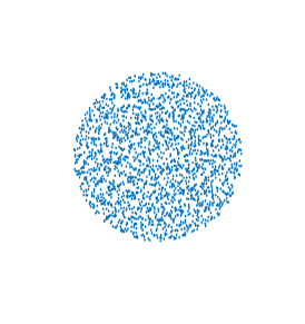
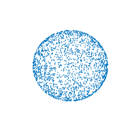
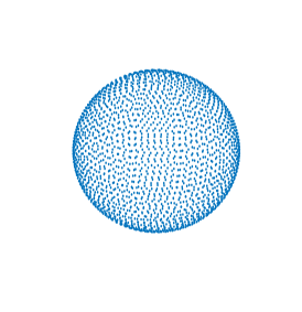
Fig. 1: Sets of collocation points: random (left), uniform (middle) and Halton (right)

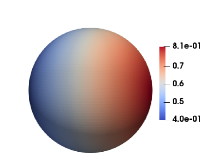
Fig. 2: Exact solution (left) and approximate solution (right).

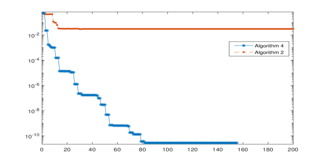
Fig. 3: Example 1: Values of the relative error versus the number of iterations.

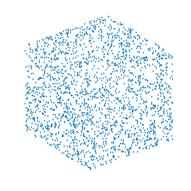
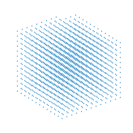
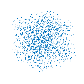
Fig. 4: Sets of collocation points: random (left), uniform (middle) and Halton (right).

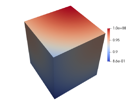
Fig. 5: Exact solution (left) and approximate solution (right).

6.2 Example 2

In this example we are interested in the numerical solution of the three-dimensional Helmholtz equation (39) in the unit cube $\Omega=[0,1]^{3}$. This geometry is displayed in Figure 1. As a test the function $f$ is specified so that the exact solution is

$$u(x,y,z)=\text{exp}\left(-\frac{x^{2}+y^{2}+z^{2}}{\sigma}\right),$$ (42)

with $\sigma=20$. Table 2 displays the performance of Algorithm 2 and Algorithm 4. In Algorithm 2, we have used as an input for noise level $\nu=10^{-3}$, $\mathscr{C}$, $\mathscr{X}_{0}=\mathscr{O}$, $tol=10^{-6}$, $m=10$ and $\text{Iter}_{\text{max}}=10$. The chosen inner and outer iterations were $m=4$ and $\text{Iter}_{\text{max}}=4$, respectively. For the ten outer iterations, minimizing the GCV function produces $\mu_{10}=1.15\times 10^{-5}$.

Collocation points	$M=N=P$	Method	Relative error	CPU-time (sec)
$\tt Random$	$10$	Algorithm 2	$4.59\times 10^{-2}$	$1.15$
		Algorithm 4	$2.64\times 10^{-10}$	$0.73$
	$20$	Algorithm 2	$4.12\times 10^{-2}$	$13.22$
		Algorithm 4	$5.12\times 10^{-11}$	$6.02$
$\tt Uniform$	$10$	Algorithm 2	$4.11\times 10^{-2}$	$0.22$
		Algorithm 4	$1.15\times 10^{-6}$	$1.64$
	$20$	Algorithm 2	$5.69\times 10^{-1}$	$14.65$
		Algorithm 4	$2.17\times 10^{-6}$	$4.80$
$\tt Halton$	$10$	Algorithm 2	$1.17\times 10^{-1}$	$1.15$
		Algorithm 4	$4.49\times 10^{-5}$	$1.28$
	$20$	Algorithm 2	$1.60\times 10^{-1}$	$13.65$
		Algorithm 4	$4.50\times 10^{-5}$	$18.19$

Table 2: Results for Example 2.

6.3 Example 3

In this example, we illustrate the efficiency of Algorithm 4 applied to solving ill-posed tensor problem (20) resulting from MQ-RBF discretization of a real-world problem of industrial relevance. We consider the geometry corresponding to a a pump casing model created by using the Gmsh tool [21]. Several methods have been proposed in the literature to comprehensively study the acoustic behaviors of the pump casing [22, 23]. The boundary of the pump model displayed in Figure 6. We consider 432124 collocation points. Problems of such large size add another level of difficulty to our methods, for example, we are unable to store the underlying tensors $\mathcal{A}$ and $\mathcal{H}$ in memory. To overcome this we resort to the hierarchical MQ-RBF interpolation based compression technique described in Section 4. Specifically. Here, we consider Dirichlet boundary conditions, i.e., (40) with $a(x)=1$ and $b(x)=0,$. The analytical solution is given by

$$u(x,y,z)=\text{exp}\left(-\frac{(x-1.75)^{2}+y^{2}+(z-0.1)^{2}}{\sigma_{1}}\right)+\text{exp}\left(-\frac{x^{2}+y^{2}+z^{2}}{\sigma_{2}}\right),$$ (43)

with $\sigma_{1}=\sigma_{2}=0.5$. Algorithm 4 terminates after 44 steps of Einstein Tensor Global Golub Kahan algorithm to reach $\tau=10^{-12}$, and the computed approximate solution $\mathcal{X}_{44}$, defined by (36). The relative error corresponding to the computed solution is given by $\frac{\left\|{\mathcal{U}}-{\mathcal{U}}_{\text{computed}}\right\|_{F}}{\|{\mathcal{U}}\|_{F}}=1.32\times 10^{-9}.$ The computed solution is shown in Figure 7.

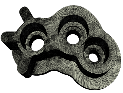
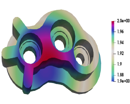
Fig. 6: Geometry of the thermal model of a pump casing (left) and exact solution (right).

Fig. 7: Approximate solution obtained by Algorithm 4.

7 Conclusion

In this paper we have proposed tensor version of GMRES and Golub–Kahan bidiagonalization algorithms using the T-product, with applications to solving large-scale linear tensor equations arising in the reconstructions of blurred and noisy multichannel images and videos. The numerical experiments that we have performed show the effectiveness of the proposed schemes to inexpensively computing regularized solutions of high quality.

References

- [1] M. Aussal, The gypsilabtoolbox for matlab version 0.5. openhmx library., Centre de Mathematiques Appliquees, Ecole polytechnique, route de Saclay, 91128 Palaiseau, France
- [2] R.K. Beatson, J.B. Cherrie and C.T. Mouat, Fast fitting of radial basis functions: method based on preconditioned GMRES iteration, Adv. Comput. Math. 11(1999), pp. 253–270
- [3] A.H. Bentbib, M. El Guide, K. Jbilou and L. Reichel, Global Golub–Kahan bidiagonalization applied to large discrete ill-posed problems, Journal of Computational and Applied Mathematics, 322(2017), 46–56.
- [4] A.H. Bentbib, M. El Guide, K. Jbilou, E. Onunwor and L. Reichel, Solution methods for linear discrete ill-posed problems for color image restoration, BIT Numerical Mathematics, 58(3)(2018), 555–-576.
- [5] K. Braman, Third-order tensors as linear operators on a space of matrices, Lin. Alg. Appl. 433(2010), 1241–1253.
- [6] M. Brazell, N. Li. C. Navasca, C. Tamon, Solving Multilinear Systems Via Tensor Inversion SIAM J. Matrix Anal. Appl., 34(2)(2013), 542–570
- [7] R. Bouyouli, K. Jbilou, R. Sadaka, H. Sadok, Convergence properties of some block Krylov subspace methods for multiple linear systems, J. Comput. Appl. Math. 196(2006), 498–511.
- [8] F. P. A Beik, F. S. Movahed, S. Ahmadi-Asl, On the Krylov subspace methods based on tensor format for positive definite Sylvester tensor equations, Numer. Lin. Alg. Appl., 23(2016), 444–466.
- [9] F. P. A. Beik, K. Jbilou, M. Najafi-Kalyani and L. Reichel, Golub–Kahan bidiagonalization for ill-conditioned tensor equations with applications. Numerical Algorithms (2020), doi.org/10.1007/s11075-020-00896-8.
- [10] A. Bouhamidi, K. Jbilou, A Sylvester-Tikhonov regularization method for image restauration, J. Compt. Appl. Math., 206(2007), 86–98.
- [11] D. Calvetti, P. C. Hansen, and L. Reichel, L-curve curvature bounds via Lanczos bidiagonalization, Electron. Trans. Numer. Anal., 14(2002), 134–149.
- [12] D. Calvetti and L. Reichel, Tikhonov regularization with a solution constraint, SIAM J. Sci. Comput., 26(2004), 224–239.
- [13] D. Calvetti, G. H. Golub, and L. Reichel, Estimation of the L-curve via Lanczos bidiagonalization, BIT, 39(1999), 603–619.
- [14] A. Einstein, The foundation of the general theory of relativity. In: Kox AJ, Klein MJ, Schulmann R, editors. The collected papers of Albert Einstein. Vol. 6, Princeton (NJ): Princeton University Press; 2007, pp. 146–200.
- [15] C. Fenu, D. Martin, L. Reichel, and G. Rodriguez, Block Gauss and anti-Gauss quadrature with application to networks, SIAM J. Matrix Anal. Appl.,, 34(4)(2013) 1655–1684
- [16] M. El Guide, A. El Ichi, K. Jbilou, F.P.A Beik, Tensor GMRES and Golub-Kahan Bidiagonalization methods via the Einstein product with applications to image and video processing, arXiv preprint arXiv:2005.07458.
- [17] A. El ichi, K. Jbilou, R. Sadaka, Tensor Krylov subspace methods using the T-product, preprint arxiv 2020.
- [18] G. E. Fasshauer, Meshfree Approximation Methods with Matlab. World Scientific, 2007.
- [19] G. H. Golub and C. F. Van Loan, Matrix Computations, 3rd ed., Johns Hopkins University Press, Baltimore, 1996.
- [20] G. H. Golub, M. Heath, G. Wahba, Generalized cross-validation as a method for choosing a good ridge parameter, , Technometrics 21(1979), 215–223.
- [21] Geuzaine C, Remacle JF. Gmsh: a three-dimensional finite element mesh generator with built-in pre- and post-processing facilities. International Journal for Numerical Methods in Engineering 2009; 79(11):1309–1331
- [22] A. Vacca, M. Guidetti, Modelling and experimental validation of external spur gear machines for fluid power applications, Elsevier Simul. Model. Pract. Theory 19 (2011) 2007–2031.
- [23] Tang C , Wang YS , Gao JH , Guo H . Fluid-sound coupling simulation and experimental validation for noise characteristics of a variable displacement external gear pump. Noise Control Eng J 2014;62(3):123–131 .
- [24] G.M.L. Gladwell and N.B. Willms, On the mode shape of the Helmholtz equation, J. Sound Vib. 188 (1995), pp. 419–433.
- [25] P. C. Hansen Analysis of discrete ill-posed problems by means of the L-curve, SIAM Rev., 34(1992), 561-580.
- [26] P. C. Hansen Regularization tools, a MATLAB package for analysis of discrete regularization problems, Numer. Algo., 6 (1994), 1-35.
- [27] N. Hao, M. E. Kilmer, K. Braman and R. C. Hoover, Facial recognition using tensor-tensor decompositions, SIAM J. Imaging Sci., 6(2013), 437–463.
- [28] R. Hardy, Multiquadric equations of topography and other irregular surfaces, J. Geophys. Res. 76(1971), pp. 1905-1915.
- [29] Huang B, Xie Y, Ma C. Krylov subspace methods to solve a class of tensor equations via the Einstein product. Numer Linear Algebra Appl. 2019;26:e2254.
- [30] P. C. Hansen, J. Nagy, and D. P. O’Leary, Deblurring Images: Matrices, Spectra, and Filtering, SIAM, Philadelphia, 2006.
- [31] K. Jbilou A. Messaoudi H. Sadok Global FOM and GMRES algorithms for matrix equations, Appl. Num. Math., 31(1999), 49–63.
- [32] K. Jbilou, H. Sadok, and A. Tinzefte, Oblique projection methods for linear systems with multiple right-hand sides, Electron. Trans. Numer. Anal., 20(2005) ,119–138.
- [33] M. N. Kalyani, F. P. A. Beik and K. Jbilou, On global iterative schemes based on Hessenberg process for (ill-posed) Sylvester tensor equations, J. Comput. Appl. Math. 373(2020), 112216.
- [34] T. G. Kolda, B. w. Bader, Tensor Decompositions and Applications. SIAM Rev. 3, 455-500 (2009).
- [35] T. Kolda, B. Bader, Higher-order web link analysis using multilinear algebra, in: Proceedings of the Fifth IEEE International Conference on Data Mining, ICDM 2005, IEEE Computer Society, 2005, pp. 242–-249.
- [36] M.E. Kimler and C.D. Martin Factorization strategies for third-order tensors, Lin. Alg. Appl., 435(2011), 641–-658.
- [37] M.E. Kilmer, C.D. Martin, L. Perrone, A third-order generalization of the matrix svd as a product of third-order tensors, Tech. Report TR-2008-4, Tufts University, Computer Science Department, 2008.
- [38] M. E. Kilmer, K. Braman, N. Hao and R. C. Hoover, Third-order tensors as operators on matrices: a theoretical and computational framework with applications in imaging, SIAM J. Matrix Anal. Appl., 34(2013), 148–172.
- [39] M. Liang, B. Zheng, Further results on Moore–Penrose inverses of tensors with application to tensor nearness problems. Comput. Math. Appl., 77(5)(2019), 1282–1293.
- [40] N. Lee, A. Cichocki, Fundamental tensor operations for large-scale data analysis using tensor network formats, Mult. Sys.t Sig.n Pro., 29(2018), 921–960.
- [41] Qi, L.-Q., Luo, Z.-Y.: Tensor analysis: spectral theory and special tensors. SIAM, Philadelphia, 2017.
- [42] G. R. Liu, Mesh Free Methods: Moving beyond the Finite Element Method, CRC Press 2002 (Boca Raton, FL).
- [43] Tensor Robust Principal Component Analysis with A New Tensor Nuclear Norm, IEEE trans. Patt. Anal. Mach. Intel.,
- [44] L. De Lathauwer and A. de Baynast, Blind deconvolution of DS-CDMA signals by means of decomposition in rank-(l, L, L) terms, IEEE Trans. Sign.Proc., 56(2008), 1562–1571.
- [45] Liu, Y., Sid-Lakhdar, W., Rebrova, E., Ghysels, P., and Li, X. S.X. A parallel hierarchical blocked adaptive cross approximation algorithm. The International Journal of High Performance Computing Applications, 34(4) 2020, 394–408.
- [46] Li, X.-T., Ng, M.K.: Solving sparse non-negative tensor equations: algorithms and applications. Front. Math. China 10(3)(2015), 649–-680.
- [47] Luo, Z.-Y., Qi, L.-Q., Xiu, N.-H.: The sparsest solutions to Z-tensor complementarity problems. Optim Lett. 11(2017), 471–-482.
- [48] Y. Miao, L. Qi and Y. Wei, Generalized Tensor Function via the Tensor Singular Value Decomposition based on the T-Product, Lin. Alg. Appl., 590(2020), 258–303.
- [49] S. Sarra and E. Kansa , Multiquadric Radial Basis Function Approximation Methods for the Numerical Solution of Partial Differential Equations (Advances in Computational Mechanics vol 2) ed Atluri S N (Tech Science Press) 2009.
- [50] L. Sun, B. Zheng, C.Bu, Y.Wei, Moore Penrose inverse of tensors via Einstein product, Lin. Mult. Alg, 64(2016),686–698.
- [51] A.N. Tikhonov, Regularization of incorrectly posed problems, Soviet Math., 4(1963), 1624–1627.
- [52] M. A. O. Vasilescu and D. Terzopoulos, Multilinear analysis of image ensembles: TensorFaces, in ECCV 2002: Proceedings of the 7th European Conference on Computer Vision, Lecture Notes in Comput. Sci. 2350, Springer, 2002, pp. 447-460.
- [53] M. A. O. Vasilescu and D. Terzopoulos, Multilinear image analysis for facial recognition, in ICPR 2002: Proceedings of the 16th International Conference on Pattern Recognition, 2002, pp. 511-514.
- [54] G. Wahba, Pratical approximation solutions to linear operator equations when the data are noisy, SIAM J. Numer. Anal. 14(1977), 651–667.
- [55] H. Wendland,Scattered Data Approximation, Cambridge University Press, 2005.
- [56] A.S. Wood, G.E. Tupholme, M.I.H. Bhatti and P.J. Heggs, Steady-state heat transfer through extended plane surfaces, Int. Commun. Heat Mass Transfer 22 (1995), pp. 99–109.