Effective Theory of Inflationary Magnetogenesis and Constraints on Reheating

Abstract

Effective theory framework based on symmetry has recently gained widespread interest in the field of cosmology. In this paper, we apply the same idea on the genesis of the primordial magnetic field and its evolution throughout the cosmological universe. Given the broken time-diffeomorphism symmetry by the cosmological background, we considered the most general Lagrangian of electromagnetic and metric fluctuation up to second order, which naturally breaks conformal symmetry in the electromagnetic (EM) sector. We also include parity violation in the electromagnetic sector with the motivation that has potential observational significance. In such a set-up, we explore the evolution of EM, scalar, and tensor perturbations considering different observational constraints. In our analysis we emphasize the role played by the intermediate reheating phase which has got limited interest in all the previous studies. Assuming the vanishing electrical conductivity during the entire period of reheating, the well-known Faraday electromagnetic induction has been shown to play a crucial role in enhancing the strength of the present-day magnetic field. We show how such physical effects combined with the PLANCK and the large scale magnetic field observation makes a large class of models viable and severely restricts the reheating equation of state parameter within a very narrow range of $0.01<\omega_{\mathrm{eff}}<0.27$, which is nearly independent of reheating scenarios we have considered.

1 Introduction

Magnetic fields are observed over a wide range of scales in our universe. They have been detected in intergalactic voids, within galaxy clusters and even in individual galaxies Grasso:2000wj ; Beck:2000dc ; Widrow:2002ud ; Kandus:2010nw ; Durrer:2013pga ; Subramanian:2015lua . Physical mechanism of the origin of such magnetic fields across wide range of scales has not been completely understood. There are two approaches which have been widely discussed in the literature. Specifically for the magnetic field at the astrophysical scale, physical processes such as Biermann battery Biermann play crucial role in providing seed fields which are subsequently amplified by dynamo mechanism in the plasma Kulsrud:2007an ; Brandenburg:2004jv ; Subramanian:2009fu .The second approach deals with the primordial generation of seed magnetic fields during inflationary phase Sharma:2017eps ; Sharma:2018kgs ; Jain:2012ga ; Durrer:2010mq ; Kanno:2009ei ; Campanelli:2008kh ; Demozzi:2009fu ; Bamba:2008ja ; Bamba:2008xa ; Bamba:2012mi ; Bamba:2006ga ; Bamba:2003av ; Bamba:2004cu ; Bamba:2020qdj ; Haque:2020bip ; Giovannini:2020zjo ; Giovannini:2017rbc ; Giovannini:2003yn ; Kobayashi:2019uqs ; Ratra:1991bn ; Ade:2015cva ; Chowdhury:2018mhj ; Vachaspati:1991nm ; Turner:1987bw ; Takahashi:2005nd ; Agullo:2013tba ; Ferreira:2013sqa ; Atmjeet:2014cxa ; Kushwaha:2020nfa ; Sharma:2021rot ; Adshead:2015pva ; Adshead:2016iae , during contracting phase Frion:2020bxc ; Chowdhury:2016aet ; Chowdhury:2018blx ; Koley:2016jdw ; Qian:2016lbf ; Membiela:2013cea . A confirmed detection of magnetic fields in the large voids in our universe might in principle indicate their primordial origin.

Among all the proposals so far, inflationary magnetogenesis has earned a lot of attention due its simplicity and elegance. Apart from solving flatness and horizon problems of standard big-bang, inflation predicts a nearly scale invariant power spectrum of CMB and matter density distribution that are consistent with the Planck observations with great precision guth ; Linde:2005ht ; Langlois:2004de ; Riotto:2002yw ; Baumann:2009ds ; Bamba:2015uma . Therefore, same paradigm playing the role in generating large scale magnetic field would have larger theoretical motivation. The standard Maxwell’s theory is conformal invariant. Therefore, magnetic field can not be generated in the conformally flat inflationary background. The simplest way to harness electromagnetic energy from the background inflaton energy, therefore, is to break this conformal invariance. Several magnetogenesis models have been proposed along this line where the conformal invariance is broken by introducing explicit coupling between EM field with inflaton, axion, or higher curvature term. Sharma:2017eps ; Sharma:2018kgs ; Jain:2012ga ; Durrer:2010mq ; Kanno:2009ei ; Campanelli:2008kh ; Demozzi:2009fu ; Bamba:2008ja ; Bamba:2008xa ; Bamba:2012mi ; Bamba:2006ga ; Bamba:2003av ; Bamba:2004cu ; Bamba:2020qdj ; Haque:2020bip ; Giovannini:2020zjo ; Giovannini:2017rbc ; Giovannini:2003yn ; Kobayashi:2019uqs ; Ratra:1991bn ; Ade:2015cva ; Chowdhury:2018mhj ; Vachaspati:1991nm ; Turner:1987bw ; Takahashi:2005nd ; Agullo:2013tba ; Ferreira:2013sqa ; Atmjeet:2014cxa ; Kushwaha:2020nfa ; Sharma:2021rot ; Adshead:2015pva ; Adshead:2016iae ; Caprini:2014mja ; Kobayashi:2014sga ; Atmjeet:2013yta ; Fujita:2015iga ; Campanelli:2015jfa ; Tasinato:2014fia . However this simple mechanism of inflationary magnetogenesis is riddled with some obvious theoretical problems. Those are related to backreaction and the strong coupling problems. The backreaction problem arises when the EM field energy density overshoots the background energy density, by which the inflationary evolution of the scale factor may be spoiled. On other hand, the strong coupling problem occurs when the effective electric charge becomes strong during inflation, which makes the perturbative calculation questionable. Thus in order to ensure the viability of an inflationary magnetogenesis model, the backreaction and the strong coupling issues should be addressed and resolved in the model (see Sharma:2017eps ; Demozzi:2009fu ; Ferreira:2013sqa ; Tasinato:2014fia ).

Apart from the inflationary perspective, the magnetic field generation in the context of bouncing cosmology has also been proposed earlier in the literature Frion:2020bxc ; Chowdhury:2016aet ; Chowdhury:2018blx ; Koley:2016jdw ; Qian:2016lbf ; Membiela:2013cea . However, it may be mentioned that in spite of predicting scale invariant power spectrum(s) consistent with the Planck observations, the bouncing model(s), generally, suffers from important theoretical issues such as violation of energy condition at the bounce point, the BKL instability associated with the growth of anisotropy at the contracting stage of the universe, the instability of the scalar and tensor perturbations etc Brandenberger:2012zb ; Brandenberger:2016vhg ; Battefeld:2014uga ; Novello:2008ra ; Cai:2014bea ; Nojiri:2019lqw ; Odintsov:2015ynk . Such problems can be rescued to some extend in some modified theories of gravity including the higher curvature theories or extra dimensional model Battefeld:2014uga ; Cai:2008qw ; Elizalde:2019tee ; Elizalde:2020zcb ; Navo:2020eqt ; Bamba:2014mya ; Odintsov:2020zct ; Banerjee:2020uil .

The Effective Field Theory (EFT) of cosmology is extremely powerful and has been widely used to study inflation Cheung:2007st ; Weinberg:2008hq ; Qiu:2020qsq , bounce Cai:2016thi ; Cai:2017tku and dark energy Gubitosi:2012hu ; Gleyzes:2013ooa ; Piazza:2013coa . Motivated by these works, in the present paper, we explore the inflationary magnetogenesis from the EFT perspective. Our basic framework would be effective theory of inflationary fluctuations coupled with the electromagnetic field. Time dependent inflaton background naturally breaks time diffeomorphism keeping spatial diffeomorphism intact. Using this spatial diffeomorphism symmetry, most general effective action for the metric perturbation coupled with the EM field can be written. Apart from the coupling with the spacetime perturbation, the EM field action also has self interaction terms which behave as scalar quantity under the spatial diffeomorphism symmetry transformation. Such self interaction couplings, along with that with the spacetime perturbation, spoil the conformal invariance in the EM sector and eventually leads to the gauge field production from primordial vacuum. In such a set-up, we have explored the evolution of the EM, scalar and tensor perturbation fields throughout cosmological evolution starting from the inflationary era. In this regard, we discuss two different scenarios depending on whether the magnetic power spectrum or the electric power spectrum become scale invariant in the inflationary superhorizon scale. After the inflationary epoch, the universe enters into a reheating era, and based on the reheating dynamics, we consider two different cases: (i) Firstly we assume an instantaneous reheating scenario where the universe makes a sudden jump from the inflationary epoch to the radiation dominated epoch, (ii) In the second case we consider the universe undergoing a reheating phase with non-zero e-fold number. In particular, we consider the conventional reheating mechanism where the inflaton field instantaneously converts to radiation energy density at the end of reheating, as proposed by Kamionkowski et al. Dai:2014jja (see also Cook:2015vqa ). In such scenario, the main idea is to parameterize the reheating phase by a constant effective equation of state. (iii) Finally we consider perturbative reheating scenario where the inflaton continuously decays into radiation and thus the effective equation of state during reheating becomes time dependent Albrecht:1982mp ; Ellis:2015pla ; Ueno:2016dim ; Eshaghi:2016kne ; Maity:2018qhi ; Haque:2020zco ; Haque:2019prw ; Maity:2019ltu ; Maity:2018exj ; Maity:2018dgy ; Maity:2016uyn ; Bhattacharjee:2016ohe ; DiMarco:2017zek ; Drewes:2017fmn ; DiMarco:2018bnw . Because of the qualitative differences in the aforementioned two reheating scenarios, quantitatively different constraints on the effective theory as well as reheating parameters can be observed. For example, the presence of the reheating phase with a non-zero e-fold number has been shown to enhance the strength of the magnetic field as opposed to the instantaneous reheating case. Considering both CMB and large scale magnetic field observations this will naturally put constraints on the model parameters depending on the reheating mechanisms.

The paper is organized as follows: after describing the model in Sec.2, we give the general expressions for the power spectra of EM, scalar and tensor perturbation fields in the present context in Sec.3. The solution for the vector potential and the metric perturbation variables during inflation are presented in Sec.4. The qualitative features of two different scenarios depending on whether the magnetic power spectrum or the electric power spectrum become scale invariant are carried out in Sec.5 and Sec.6 respectively, considering conventional instantaneous reheating model. In Sec.7, the present value of the magnetic field has been calculated considering conventional reheating phase wherein two possbilities with constant and time dependent reheating equation of state have been considered separately. Finally we summarise our results with some future works to be done.

2 The model

We start with the following effective field theory action,

$$S=S_{bg}+S_{em}+S_{sp}+S_{int},$$ (1)

with $S_{bg}$ denotes the background action, $S_{em}$ is the electromagnetic field action, $S_{sp}$ symbolizes the action of the metric perturbation and $S_{int}$ represents the interaction between the the electromagnetic field and the metric perturbation variable. Following idea of effective field theory (EFT) inflation Cheung:2007st ; Weinberg:2008hq , the background action is expressed as,

$$S_{bg}=\int d^{4}x\sqrt{-g}\bigg{[}\frac{1}{2}M_{\mathrm{Pl}}^{2}R-\Lambda(\eta)-c(\eta)g^{00}\bigg{]}\leavevmode\nobreak\ \leavevmode\nobreak\ \leavevmode\nobreak\ .$$ (2)

where $M_{\mathrm{Pl}}$ is the Planck mass and $R$ is the Ricci scalar. Moreover, $f(\eta)$, $\Lambda(\eta)$ and $c(\eta)$ are the background EFT parameters and can be fixed by the background equations. The metric component $g^{00}$ is one of the scalars under spacial diffeomophism symmetry $x^{i}=x^{i}+\xi^{i}(x,t)$, where $\xi^{i}$ is arbitray spatial vector. For our present purpose we consider a spatially flat FLRW background metric,

$$ds^{2}=-dt^{2}+a^{2}(t)\delta_{ij}dx^{i}dx^{j}=a^{2}(\eta)(-d\eta^{2}+\delta_{ij}dx^{i}dx^{j})\leavevmode\nobreak\ \leavevmode\nobreak\ .$$ (3)

with $\eta$ being the conformal time and related to the cosmic time ($t$) as $\eta=\int{dt}/{a(t)}$. The above FRW metric along with the action (2) immediately lead to the background Friedmann equations as,

$$3M_{\mathrm{Pl}}^{2}\mathcal{H}^{2}=a^{2}(\eta)\bigg{(}c(\eta)+\Lambda(\eta)\bigg{)}$$

$$-M_{\mathrm{Pl}}^{2}\bigg{(}2\mathcal{H}^{\prime}+\mathcal{H}^{2}\bigg{)}=a^{2}(\eta)\bigg{(}c(\eta)-\Lambda(\eta)\bigg{)},$$ (4)

where $\mathcal{H}={a^{\prime}}/{a}$ is known as the conformal Hubble parameter which is related to the cosmic Hubble parameter ($H=\dot{a}/a$) as: $\mathcal{H}=aH$ (from now onwards, a prime represents $\frac{d}{d\eta}$ and an overdot symbolizes $\frac{d}{dt}$). Here it may be interesting to present few modified gravity models and its mapping with model independent EFT framework (Eq.2). Comparing the Friedmann Eqs.(4) with that of a specific gravity model, one can get certain forms of the functions $c(\eta)$ and $\Lambda(\eta)$ correspond to the respective model. For example, scalar-Einstein-Gauss-Bonnet gravity theory, which can be consistent with Planck results for suitable choices of the Gauss-Bonnet coupling function and the scalar field potential Li:2007jm ; Odintsov:2018nch ; Carter:2005fu ; Nojiri:2019dwl ; Elizalde:2010jx ; Makarenko:2016jsy ; delaCruzDombriz:2011wn ; Bamba:2007ef ; Chakraborty:2018scm ; Kanti:2015pda ; Kanti:2015dra ; Odintsov:2018zhw ; Saridakis:2017rdo ; Cognola:2006eg , is described by the following time dependent effective theory parameters,

$$c(\eta(t)) = \frac{1}{2}\dot{\phi}^{2}-4H^{2}\ddot{h}-8H\dot{H}\dot{h}+4H^{3}\dot{h}$$

$$\Lambda(\eta(t)) = V(\phi)+4H^{2}\ddot{h}+8H\dot{H}\dot{h}+20H^{3}\dot{h}$$ (5)

where $\phi$ is the scalar field under consideration (generally the inflaton field), $V(\phi)$ and $h(\phi)$ denote the scalar field potential and the Gauss-Bonnet coupling function (with the scalar field) respectively. Thereby the scalar-Einstein-Gauss-Bonnet model is mapped into the EFT action (2) with the above expression for $c(\eta)$ and $\Lambda(\eta)$. Similarly the $F(R)$ gravity theory Nojiri:2010wj ; Nojiri:2017ncd ; Capozziello:2011et ; Elizalde:2018rmz can be embedded within the EFT action (2) for the following forms of $c(\eta)$ and $\Lambda(\eta)$ as,

$$c(\eta(t)) = \dot{H}f^{\prime}(R)+3\big{(}\dddot{H}+4\dot{H}^{2}+3H\dot{H}-4H^{2}\dot{H}\big{)}f^{\prime\prime}(R)+18\big{(}4H\dot{H}+\ddot{H}\big{)}^{2}f^{\prime\prime\prime}(R)$$ (6)

$$\Lambda(\eta(t)) = -\frac{f(R)}{2}+\big{(}2\dot{H}+3H^{2}\big{)}f^{\prime}(R)-3\big{(}\dddot{H}+4\dot{H}^{2}+9H\dot{H}+20H^{2}\dot{H}\big{)}f^{\prime\prime}(R)-18\big{(}4H\dot{H}+\ddot{H}\big{)}^{2}f^{\prime\prime\prime}(R)$$

respectively, with $f(R)$ being the correction of $F(R)$ over Einstein gravity, i.e $f(R)=F(R)-R$. Moreover in the context of holographic inflation Nojiri:2019kkp ; Nojiri:2020wmh , $c(\eta)$ and $\Lambda(\eta)$ in turn determine the corresponding holographic cut-off.
Coming back to the electromagnetic field action (i.e the second term in the right hand side of Eq.(1)), $S_{em}$ is taken as,

$$S_{em}=\int d^{4}x\sqrt{-g}\bigg{[}-\frac{1}{4}f_{1}(\eta)F_{\mu\nu}F^{\mu\nu}+f_{2}(\eta)F^{0}_{i}F^{0i}+f_{3}(\eta)\epsilon^{ijk}F^{0}_{i}F_{jk}+f_{4}(\eta)\epsilon^{\mu\nu\alpha\beta}F_{\mu\nu}F_{\alpha\beta}\bigg{]}$$ (7)

where $F_{\mu\nu}=\partial_{\mu}A_{\nu}-\partial_{\nu}A_{\mu}$ is the field strength tensor of the electromagnetic field $A_{\mu}$. Following the same argument as mentioned for $g^{00}$ metric component, $A^{0}$ component of the $A_{\mu}$ will be invariant under special diffeomorphism transformation. $f_{i}(\eta)$ ($i=1,2,3,4$) are arbitrary analytic functions of $\eta$ and denote the non-minimal coupling of the electromagnetic field. Such time dependent coupling functions naturally break the conformal invariance in the electromagnetic sector and lead to the gauge field production from primordial quantum vacuum. It may be observed that $S_{em}$ consists of all possible electromagnetic terms (up to second order) which behave as scalar quantity under the spatial diffeomorphism. Moreover at later stage, we will consider the functions $f_{i}(\eta)$ in such a way that in the early universe, the couplings introduce a non-trivial correction to the electromagnetic field evolution, while at late times specifically at the end of inflation, $f_{i}(\eta)$ will turn out to be $f_{1}(\eta)=1$, $f_{2}(\eta)=f_{3}(\eta)=f_{4}(\eta)=0$ leadin to standard Maxwellian evolution.

The spacetime perturbation action $S_{sp}$, following the line of EFT, is given by,

$$S_{sp}=\int d^{4}x\sqrt{-g} \bigg{[} \frac{M_{2}^{4}(\eta)}{2}\big{(}\delta g^{00}\big{)}^{2}-\frac{m_{3}^{3}(\eta)}{2}\delta K\delta g^{00}-m_{4}^{2}(\eta)\big{(}\delta K^{2}-\delta K_{\mu\nu}\delta K^{\mu\nu}\big{)}+\frac{\tilde{m}_{4}^{2}(\eta)}{2}R^{(3)}\delta g^{00}$$ (8)

$$- \bar{m}_{4}^{2}(\eta)\delta K^{2}-\frac{m_{5}(\eta)}{2}R^{(3)}\delta K-\frac{\lambda_{1}(\eta)}{2}\big{(}R^{(3)}\big{)}^{2}-\frac{\lambda_{2}(\eta)}{2}\nabla_{i}R^{(3)}\nabla^{i}R^{(3)}\bigg{]}$$

where all the coefficients are allowed to vary with $\eta$. All EFT parameters are so chosen that dimensions $[m_{i}]=1$ and $[\lambda_{i}]=0$. In the above expression, $\delta K_{\mu\nu}=K_{\mu\nu}-H\sigma_{\mu\nu}$, $\delta K=K-3H$ where $K_{\mu\nu}$ and $\sigma_{\mu\nu}$ are the extrinsic curvature and induced metric on a constant time hypersurface respectively. Moreover $\delta g^{00}$ is connected to the curvature perturbation variable $\Psi(\vec{x},\eta)$ by a non-trivial way which we will introduce later. The quadratic action of $\Psi(\vec{x},\eta)$ from Eq.(8) contains terms like $\big{(}\partial\Psi(\vec{x},\eta)\big{)}^{2}$, $\big{(}\partial^{2}\Psi(\vec{x},\eta)\big{)}^{2}$ and $\big{(}\partial^{3}\Psi(\vec{x},\eta)\big{)}^{2}$; which, upon Fourier transformation behave as, $\big{(}\partial\Psi\big{)}^{2}\sim k^{2}\Psi_{k}^{2}$, $\big{(}\partial^{2}\Psi\big{)}^{2}\sim k^{4}\Psi_{k}^{2}$ and $\big{(}\partial^{3}\Psi\big{)}^{2}\sim k^{6}\Psi_{k}^{2}$ respectively. Where $\Psi_{k}(\eta)$ is the Fourier mode with momentum $k$. Even though they are quadratic in fluctuation, higher derivative terms will be generically suppressed by inflationary energy scale $H$. We, therefore, will consider the curvature perturbation action upto the quadratic order in $k$. Hence, we choose following condition for our subsequent discussions,Cai:2016thi ; Cai:2017tku ,

$$\bar{m}_{4}=m_{5}=\lambda_{1}=\lambda_{2}=0$$ (9)

Correspondingly $\delta g^{00}$ is related to the metric curvature perturbation by the following way Cai:2016thi ,

$$\delta g^{00}=\frac{4\bigg{(}\frac{1}{\kappa^{2}}+2m_{4}^{2}\bigg{)}}{a(\eta)\bigg{(}\frac{2H}{\kappa^{2}}+4Hm_{4}^{2}-m_{3}^{3}\bigg{)}}\leavevmode\nobreak\ \frac{\partial\Psi}{\partial\eta}$$ (10)

where ${1}/{\kappa^{2}}=M_{\mathrm{Pl}}^{2}$ and as mentioned earlier, $H$ is the Hubble parameter in cosmic time. For computational simplicity we consider inflationary phase to be nearly de-Sitter with scale factor $a(\eta)=-{1}/{H\eta}$. Now using Eqs.(9) and (10), the quadratic action $S_{sp}$ for the fluctuation becomes,

$$S[v]=\int d^{4}x\bigg{[}(v^{\prime})^{2}+\frac{z^{\prime\prime}}{z}v^{2}-c_{s}^{2}g^{ij}\partial_{i}v\partial_{j}v\bigg{]},$$ (11)

where, $v(\vec{x},\eta)$ is the Mukhanov-Sasaki variable defined as $v(\vec{x},\eta)=z(\eta)\Psi(\vec{x},\eta)=a(\eta)\sqrt{c_{1}}\leavevmode\nobreak\ \Psi(\vec{x},\eta)$. The quantity $c_{s}^{2}$ symbolizes the sound speed for the scalar perturbation and has the following expression,

$$c_{s}^{2}=\frac{1}{c_{1}}\bigg{(}\frac{c_{3}^{\prime}(\eta)}{a^{2}}-\frac{1}{\kappa^{2}}\bigg{)}$$ (12)

with $c_{1}$ and $c_{3}$ are expressed in terms of EFT parameters (i.e $M_{2}$, $m_{3}$, $m_{4}$ and $\tilde{m}_{4}$) as follows:

$$c_{1}(\eta)=\frac{\bigg{(}\frac{1}{\kappa^{2}}+2m_{4}^{2}\bigg{)}\bigg{(}3m_{3}^{6}+8M_{2}^{4}\big{[}\frac{1}{\kappa^{2}}+2m_{4}^{2}\big{]}\bigg{)}}{\bigg{(}\frac{2H}{\kappa^{2}}+4Hm_{4}^{2}-m_{3}^{3}\bigg{)}^{2}}\leavevmode\nobreak\ ;\leavevmode\nobreak\ c_{3}(\eta)=\frac{2a(\eta)\bigg{(}\frac{1}{\kappa^{2}}+2m_{4}^{2}\bigg{)}\bigg{(}\frac{1}{\kappa^{2}}+2\tilde{m}_{4}^{2}\bigg{)}}{\bigg{(}\frac{2H}{\kappa^{2}}+4Hm_{4}^{2}-m_{3}^{3}\bigg{)}}.$$ (13)

Moreover, the quadratic action for the tensor perturbation comes as,

$$S[v_{T}]=\int d^{4}x\bigg{[}(v_{T}^{\prime})^{2}+\frac{z_{T}^{\prime\prime}}{z_{T}}v_{T}^{2}-c_{T}^{2}\big{(}\partial v_{T}\big{)}^{2}\bigg{]}$$ (14)

with $z_{T}^{2}=a^{2}(\eta)\big{(}1+2\kappa^{2}m_{4}^{2}\big{)}$ and the speed of the gravitational wave ($c_{T}^{2}$) in terms of the EFT parameters is given by $c_{T}^{2}=\big{(}1+2\kappa^{2}m_{4}^{2}\big{)}^{-1}$.
Finally $S_{int}$ refers to the quadratic interaction between the electromagnetic field and $\delta g^{00}$, which, in the context of EFT has the following form,

$$S_{int}=\int d^{4}x\sqrt{-g}\bigg{[}h(\eta)\big{(}\partial_{i}\delta g^{00}\big{)}F^{0i}\bigg{]}$$ (15)

with $h(\eta)$ being the interaction coupling strength. Such interaction of electromagnetic field ($A_{\mu}$) with the curvature perturbation appears naturally in the EFT language due to the underlying spatial diffeomorphism symmetry. However, the possible interaction of $A_{\mu}$ with the tensor perturbation appears in higher order action and thus we do not consider those terms for our present study. Along with the quadratic terms with time dependent coupling functions $f_{i}(\eta)$ in Eq.(7), the term $h(\eta)\partial_{i}\delta g^{00}\leavevmode\nobreak\ F^{0i}$ (present in $S_{int}$) also contributes in breaking the conformal invariance of the electromagnetic field action. In terms of the Mukhanov-Sasaki variable, Eq.(15) can be written as,

$$S_{int}=-2\int d^{4}x\frac{h(\eta)B(\eta)}{a(\eta)\leavevmode\nobreak\ z(\eta)}\leavevmode\nobreak\ \partial_{i}\big{[}v^{\prime}-\frac{z^{\prime}}{z}v\big{]}\leavevmode\nobreak\ F_{0i}\leavevmode\nobreak\ \leavevmode\nobreak\ \leavevmode\nobreak\ ,\leavevmode\nobreak\ \leavevmode\nobreak\ \leavevmode\nobreak\ \leavevmode\nobreak\ \leavevmode\nobreak\ \leavevmode\nobreak\ \leavevmode\nobreak\ \mathrm{with}\leavevmode\nobreak\ \leavevmode\nobreak\ \leavevmode\nobreak\ \leavevmode\nobreak\ \leavevmode\nobreak\ B(\eta)=\frac{4\bigg{(}\frac{1}{\kappa^{2}}+2m_{4}^{2}\bigg{)}}{\bigg{(}\frac{2H}{\kappa^{2}}+4Hm_{4}^{2}-m_{3}^{3}\bigg{)}}$$ (16)

Thus as a whole, $S_{bg}$, $S_{em}$, $S_{sp}$ and $S_{int}$ are given in Eqs.(2), (7), (8) and (16) respectively. In such scenario, we aim to study inflationary magnetogenesis. In this regard let us point out some salient features of the model - (i) the present magnetogenesis scenario will consider the coupled evolution of electromagnetic field and the spacetime perturbation, where, in particular, the electromagnetic field gets coupled with the curvature perturbation. However the tensor perturbation evolves freely as it does not interact either with the electromagnetic field or with the scalar perturbation upto the quadratic order. (2) The time dependent self coupling of electromagnetic field denoted by the coupling strengths $f_{i}(\eta)$ and the interaction term with $\delta g^{00}$ spoil the conformal invariance of the electromagnetic field action. The coupling strengths will be chosen in such a way that after the inflationary epoch, the conformal invariance of $A_{\mu}$ will be restored and consequently the standard Maxwell’s equations will be recovered. (3) Moreover as we will show in a later section that the well known back-reaction and strong coupling problem will be resolved in the present scenario for suitable parameter spaces.
In order to determine the equations of motion, let us recall that there are three independent fields in the model- the electromagnetic field $A_{\mu}$, the scalar and tensor Mukhanov-Sasaki variables $v(\vec{x},\eta)$ and $v_{T}(\vec{x},\eta)$ respectively. The variation of action (1) with respect to the gauge field leads to the following equation of motion for $A_{\mu}$,

$$-\partial_{a}\big{[}a^{4}(\eta)f_{1}(\eta)g^{\mu a}g^{\nu b}F_{\mu\nu}\big{]}+2\partial_{0}\big{[}f_{2}(\eta)g^{ib}\leavevmode\nobreak\ \partial_{0}A_{i}\big{]}-2\delta^{b}_{0}\leavevmode\nobreak\ \partial_{j}\big{[}f_{2}(\eta)g^{ij}\leavevmode\nobreak\ \partial_{0}A_{i}\big{]}+2\partial_{0}\big{[}a^{2}(\eta)f_{3}(\eta)\epsilon^{0bjk}\leavevmode\nobreak\ \partial_{j}A_{k}\big{]}$$ (17)

$$+ 2\partial_{j}\big{[}a^{2}(\eta)f_{3}(\eta)\epsilon^{0ijb}\leavevmode\nobreak\ \partial_{0}A_{j}\big{]}-2\delta^{b}_{0}\leavevmode\nobreak\ \partial_{i}\big{[}a^{2}(\eta)f_{3}(\eta)\epsilon^{0ijk}\leavevmode\nobreak\ \partial_{j}A_{k}\big{]}+8\partial_{a}\big{[}a^{4}(\eta)f_{4}(\eta)\epsilon^{\mu\nu\alpha\beta}\leavevmode\nobreak\ \partial_{\mu}A_{\nu}\big{]}$$

$$+ \partial_{0}\big{[}a^{2}(\eta)h(\eta)g^{ib}\leavevmode\nobreak\ \partial_{i}\delta g^{00}\big{]}=0$$

where we consider the spatially flat FRW metric ansatz as shown in Eq.(3). In the Coulomb gauge ($A_{0}=0$ and $\partial^{i}A_{i}=0$) condition, the relevant equation of motions for $A_{i}$’s are,

$$f_{1}(\eta) \big{[}A_{i}^{\prime\prime}+\frac{f_{1}^{\prime}}{f_{1}}A_{i}^{\prime}-\partial_{l}\partial_{l}A_{i}\big{]}+\frac{2}{a^{2}(\eta)}f_{2}(\eta)\leavevmode\nobreak\ \big{[}A_{i}^{\prime\prime}+\frac{f_{2}^{\prime}}{f_{2}}A_{i}^{\prime}-\frac{2a^{\prime}}{a}A_{i}^{\prime}\big{]}+\frac{2}{a^{2}}f_{3}(\eta)\epsilon_{ijk}\leavevmode\nobreak\ \big{[}\frac{f_{3}^{\prime}}{f_{3}}-\frac{2a^{\prime}}{a}\big{]}\leavevmode\nobreak\ \partial_{j}A_{k}$$ (18)

$$- 8f_{4}^{\prime}(\eta)\epsilon_{ijk}\leavevmode\nobreak\ \partial_{j}A_{k}-h(\eta)\leavevmode\nobreak\ \partial_{0}\partial_{i}\big{(}\delta g^{00}\big{)}-h^{\prime}(\eta)\leavevmode\nobreak\ \partial_{i}\big{(}\delta g^{00}\big{)}=0$$

with a prime denoting $\frac{d}{d\eta}$.

The equation of motion for the scalar and tensor perturbation will take the following form,

$$v^{\prime\prime}(\vec{x},\eta)-\frac{z^{\prime\prime}}{z}v-c_{s}^{2}\leavevmode\nobreak\ \partial_{i}\partial^{i}v=0$$ (19)

$$v_{T}^{\prime\prime}(\vec{x},\eta)-\frac{z_{T}^{\prime\prime}}{z_{T}}v_{T}-c_{T}^{2}\leavevmode\nobreak\ \partial_{i}\partial^{i}v_{T}=0\leavevmode\nobreak\ \leavevmode\nobreak\ .$$

where in the above derivation Coulomb gauge condition is used. with recall, $z(\eta)=a(\eta)\sqrt{c_{1}(\eta)}$ and $c_{s}^{2}$ is given in Eq.(12). It may be observed that the scalar perturbation evolves freely, but the electromagnetic field evolution does depend on the scalar perturbation evolution through $h(\eta)$ as evident from Eq.(18). This is due to Coulomb gauge condition. The solution of these equations require a certain ansatz of the background spacetime scale factor $a(\eta)$ and the coupling functions $f_{i}(\eta)$, $h(\eta)$. For the background spacetime, we consider a de-Sitter inflationary spacetime, in which case, the scale factor is given by,

$$a(\eta)=-\frac{1}{H\eta}\leavevmode\nobreak\ \leavevmode\nobreak\ \leavevmode\nobreak\ ,$$ (20)

with $H$ being is very slowly varying function and represents the Hubble parameter in cosmic time. The scale factor of Eq.(20) immediately leads to the Hubble parameter in conformal time as $\mathcal{H}=\frac{1}{a}\frac{da}{d\eta}=-1/\eta$. Furthermore, we introduce the inflationary e-folding number as $N(\eta)=\ln{\big{(}a(\eta)\big{)}}$, which is counted from the beginning of inflation where $N=0$ and we consider the beginning of inflation to be the instant when the CMB scale mode crosses the horizon.

Here we assume the EFT parameters are non-zero (i.e all the electromagnetic terms present in the EFT action (7) have been taken into account) and have the power law forms of the scale factor, in particular,

$$f_{1}(\eta)=\left\{\begin{array}[]{cc}\bigg{(}\frac{a(\eta)}{a_{f}(\eta_{f})}\bigg{)}^{2}&\leavevmode\nobreak\ \leavevmode\nobreak\ \leavevmode\nobreak\ \eta\leq\eta_{f}\\ 1&\leavevmode\nobreak\ \leavevmode\nobreak\ \leavevmode\nobreak\ \eta\geq\eta_{f}\end{array}\right.$$ (23)

and

$$f_{2}(\eta)=\bigg{(}\frac{a_{i}(\eta_{i})}{a(\eta)}\bigg{)}^{m}\leavevmode\nobreak\ \leavevmode\nobreak\ ;\leavevmode\nobreak\ \leavevmode\nobreak\ f_{3}(\eta)=\bigg{(}\frac{a_{i}(\eta_{i})}{a(\eta)}\bigg{)}^{r}\leavevmode\nobreak\ \leavevmode\nobreak\ ;\leavevmode\nobreak\ \leavevmode\nobreak\ f_{4}(\eta)=\bigg{(}\frac{a_{i}(\eta_{i})}{a(\eta)}\bigg{)}^{s}\leavevmode\nobreak\ \leavevmode\nobreak\ ;\leavevmode\nobreak\ \leavevmode\nobreak\ h(\eta)=h_{0}\bigg{(}\frac{a_{i}(\eta_{i})}{a(\eta)}\bigg{)}^{2}$$ (24)

where $a_{i}$ and $a_{f}$ are the scale factors at the beginning $\eta_{i}$ and at the end of inflation $\eta_{f}$ respectively. Moreover $h_{0}$ is constant having mass dimension unity. The exponents $m$, $r$, $s$ are positive numbers and can act as model parameters in the present context. Later, we will show that $m=r=s=2$ leads to a scale invariant magnetic power spectrum in the superhorizon limit. It is evident from the above expressions that $f_{1}(\eta)$ starts from $e^{-2N_{f}}$ and monotonically increases till $\eta=\eta_{f}$, while the other coupling functions monotonically decreases with time during the inflationary stage. However in the post-inflationary phase, $f_{1}(\eta)$ becomes unity and $f_{2}(\eta)\approx f_{3}(\eta)\approx f_{4}(\eta)\approx h(\eta)\approx 0$, which in turn recovers the standard Maxwell’s equations at late time.

Before embarking on our study with the aforementioned forms of the EFT parameters, let us contextualise our discussions by giving few explicit model examples with elaborate discussions given in appendix-A.
Generalized Ratra Model: In this model the conformal invariance is broken by generic scalar function as a gauge kinetic function as

$$S_{m1}=\int d^{4}x\sqrt{-g}\left[f(\phi,R,{\cal G})F_{\mu\nu}F^{\mu\nu}\right],$$ (25)

where $(\phi,R,{\cal G})$ are scalar field under consideration (generally the inflaton), the background Ricci scalar and the Gauss-Bonnet scalar respectively. The scenario with $f(\phi,R,{\cal G})=f(\phi)$ is well known Ratra model whch has been studied extensively (without or with reheating phase) in Demozzi:2009fu ; Haque:2020bip ; Kobayashi:2019uqs ; Ratra:1991bn ; moreover the case $f(\phi,R,\mathcal{G})=f(R,\mathcal{G})$ has also been explored (without or with reheating phase) in Bamba:2020qdj . Comparing the action (25) with the EFT action (7), the associated EFT parameters can be mapped as:

$$f_{1}(\eta)=f\left(\phi(\eta),R(\eta),{\cal G}(\eta)\right)\leavevmode\nobreak\ \leavevmode\nobreak\ \leavevmode\nobreak\ \leavevmode\nobreak\ \leavevmode\nobreak\ \leavevmode\nobreak\ ,\leavevmode\nobreak\ \leavevmode\nobreak\ \leavevmode\nobreak\ \leavevmode\nobreak\ \leavevmode\nobreak\ f_{2}(\eta)=f_{3}(\eta)=f_{4}(\eta)=0..$$ (26)

where $\phi(\eta)$ can be obtained from the background evolution of the scalar field over FRW spacetime, $R(\eta)=\frac{6}{a^{2}}\left(\mathcal{H}^{\prime}+\mathcal{H}^{2}\right)$ and $\mathcal{G}(\eta)=\frac{24}{a^{4}}\mathcal{H}^{2}\mathcal{H}^{\prime}$, with $\mathcal{H}$ represents the conformal Hubble parameter. One gets a further generalized scenario by adding parity violating term in the above Lagrangian, in particular,

$$S_{g}=S_{m1}+S_{pv}$$ (27)

with

$$S_{pv}=\int d^{4}x\sqrt{-g}\bigg{[}\frac{\alpha}{M^{2}}\epsilon^{\mu\nu\alpha\beta}RF_{\mu\nu}F_{\alpha\beta}+\frac{\beta}{M^{2}}\epsilon^{\mu\alpha\beta\delta}R_{\mu\nu}F_{\alpha}^{\nu}F_{\beta\delta}+\frac{\gamma}{M^{2}}\epsilon^{\mu\nu\alpha\beta}R_{\mu\nu}^{\leavevmode\nobreak\ \leavevmode\nobreak\ \rho\sigma}F_{\rho\sigma}F_{\alpha\beta}\bigg{]}$$ (28)

with $\alpha$, $\beta$ and $\gamma$ are model parameters. The background spacetime immediately leads to the Ricci scalar and the non-zero components of Ricci tensor, Riemann tensor as,

$$R = 6\frac{a^{\prime\prime}}{a^{3}}\leavevmode\nobreak\ \leavevmode\nobreak\ \leavevmode\nobreak\ \leavevmode\nobreak\ \leavevmode\nobreak\ \leavevmode\nobreak\ \leavevmode\nobreak\ ,\leavevmode\nobreak\ \leavevmode\nobreak\ \leavevmode\nobreak\ \leavevmode\nobreak\ \leavevmode\nobreak\ \leavevmode\nobreak\ \leavevmode\nobreak\ \leavevmode\nobreak\ R_{00}=-3\left(\frac{a^{\prime\prime}}{a}-\frac{a^{\prime 2}}{a^{2}}\right)\leavevmode\nobreak\ \leavevmode\nobreak\ \leavevmode\nobreak\ \leavevmode\nobreak\ \leavevmode\nobreak\ \leavevmode\nobreak\ \leavevmode\nobreak\ ,\leavevmode\nobreak\ \leavevmode\nobreak\ \leavevmode\nobreak\ \leavevmode\nobreak\ \leavevmode\nobreak\ \leavevmode\nobreak\ \leavevmode\nobreak\ R_{ij}=\left(\frac{a^{\prime\prime}}{a}+\frac{a^{\prime 2}}{a^{2}}\right)$$

$$R_{0i}^{\leavevmode\nobreak\ \leavevmode\nobreak\ 0j} = \left(\frac{a^{\prime 2}}{a^{4}}-\frac{a^{\prime\prime}}{a^{3}}\right)\delta_{i}^{j}\leavevmode\nobreak\ \leavevmode\nobreak\ \leavevmode\nobreak\ \leavevmode\nobreak\ \leavevmode\nobreak\ \leavevmode\nobreak\ \leavevmode\nobreak\ ,\leavevmode\nobreak\ \leavevmode\nobreak\ \leavevmode\nobreak\ \leavevmode\nobreak\ \leavevmode\nobreak\ \leavevmode\nobreak\ \leavevmode\nobreak\ R_{ij}^{\leavevmode\nobreak\ \leavevmode\nobreak\ kl}=\frac{a^{\prime 2}}{a^{4}}\left(\delta_{i}^{l}\delta_{j}^{k}-\delta_{i}^{k}\delta_{j}^{l}\right)\leavevmode\nobreak\ \leavevmode\nobreak\ .$$ (29)

Consequently, the action $S_{pv}$ turns out to be,

$$S_{pv} = \int d^{4}x\sqrt{-g}\bigg{[}6\frac{\alpha}{M^{2}}\epsilon^{\mu\nu\alpha\beta}\left(\frac{a^{\prime\prime}}{a^{3}}\right)F_{\mu\nu}F_{\alpha\beta}$$ (30)

$$+ \frac{1}{M^{2}}\epsilon^{ijk}\bigg{\{}2\beta\left(aa^{\prime\prime}+a^{\prime 2}\right)-3\beta\left(\frac{a^{\prime\prime}}{a}-\frac{a^{\prime 2}}{a^{2}}\right)-\gamma\left(\frac{a^{\prime\prime}}{a}+\frac{a^{\prime 2}}{a^{2}}\right)\bigg{\}}F_{i}^{0}F_{jk}\bigg{]}\leavevmode\nobreak\ \leavevmode\nobreak\ .$$

Thereby comparing the action (27) with the EFT action of Eq.(7), we argue that the action $S_{m5}$ can be embedded within the EFT action of EM field, provided the EFT parameters have the following forms,

$$f_{1}(\eta) = f\left(\phi(\eta),R(\eta),{\cal G}(\eta)\right)\leavevmode\nobreak\ \leavevmode\nobreak\ \leavevmode\nobreak\ \leavevmode\nobreak\ \leavevmode\nobreak\ \leavevmode\nobreak\ ,\leavevmode\nobreak\ \leavevmode\nobreak\ \leavevmode\nobreak\ \leavevmode\nobreak\ \leavevmode\nobreak\ \leavevmode\nobreak\ f_{2}(\eta)=0$$

$$f_{3}(\eta) = \frac{1}{M^{2}}\bigg{\{}2\beta\left(aa^{\prime\prime}+a^{\prime 2}\right)-3\beta\left(\frac{a^{\prime\prime}}{a}-\frac{a^{\prime 2}}{a^{2}}\right)-\gamma\left(\frac{a^{\prime\prime}}{a}+\frac{a^{\prime 2}}{a^{2}}\right)\bigg{\}}$$

$$f_{4}(\eta) = 6\frac{\alpha}{M^{2}}\left(\frac{a^{\prime\prime}}{a^{3}}\right)$$ (31)

respectively. By this way, one may construct more general magnetogenesis models from the EFT formalism with suitable choices of $f_{i}(\eta)$. This requires a complete scan of the EFT parameters for which the EFT action can generate sufficient magnetic strength and at the same time be self consistent, which we expect to study in future. However the present work and the following discussions are based on the EFT parameters chosen in Eqs. (23) and (24) respectively.

3 Energy density and power spectra for electromagnetic and metric perturbation fields

In the present section, we will calculate the power spectra for both the electromagnetic and metric perturbation fields. In regard to the electromagnetic field, it may be mentioned that the electric and the magnetic fields are frame dependent. In the present context, the electric and magnetic fields are referred with respect to the comoving observer, in which case the proper time becomes identical with the cosmic time or equivalently the four velocity components of a comoving observer are given by $u^{\mu}=\big{(}1/a(\eta),0,0,0\big{)}$. For the purpose of the computation of the power spectrum; first we need to know the energy density for the respective fields and, secondly, the vacuum state associated with the field in the background inflationary evolution. Thereby, from the action (1), we first determine the energy-momentum tensor associated with the electromagnetic field,

$$T_{ab} = -\frac{1}{4}f_{1}(\eta)\leavevmode\nobreak\ \big{[}g_{ab}F^{2}-4g^{\mu\alpha}F_{\mu a}F_{\alpha b}\big{]}+f_{2}(\eta)\leavevmode\nobreak\ \big{[}\frac{1}{a^{4}}g_{ab}g^{ij}F_{0i}F_{0j}-\frac{2}{a^{4}}F_{0a}F_{0b}-\frac{4}{a^{2}}\leavevmode\nobreak\ \delta^{0}_{a}g^{ij}F_{0i}F_{bj}\big{]}$$

$$+ \frac{2}{a^{4}}\leavevmode\nobreak\ f_{3}(\eta)\epsilon_{ijk}\leavevmode\nobreak\ \delta^{0}_{a}\ F_{bi}F_{jk}+h(\eta)\leavevmode\nobreak\ \big{[}g_{ab}g^{0\mu}g^{i\nu}F_{\mu\nu}\leavevmode\nobreak\ \partial_{i}\big{(}\delta g^{00}\big{)}-2\delta^{0}_{a}g^{i\nu}F_{b\nu}\leavevmode\nobreak\ \partial_{i}\big{(}\delta g^{00}\big{)}-2g^{0\mu}F_{\mu b}\leavevmode\nobreak\ \partial_{a}\big{(}\delta g^{00}\big{)}\big{]}$$

The energy density of the EM field in the background FRW spacetime is given by $T^{0}_{0}=-\frac{1}{a^{2}}T_{00}$ and thus the above expression of $T_{\alpha\beta}$ immediately leads to the following form of $T^{0}_{0}$:

$$T^{0}_{0} = f_{1}(\eta)\leavevmode\nobreak\ \big{[}-\frac{1}{2a^{4}}(A_{i}^{\prime})^{2}-\frac{1}{4a^{4}}F_{ij}F_{ij}\big{]}+f_{2}(\eta)\leavevmode\nobreak\ \big{[}-\frac{3}{a^{6}}(A_{i}^{\prime})^{2}\big{]}$$

$$+ f_{3}(\eta)\leavevmode\nobreak\ \big{[}-\frac{4}{a^{6}}\epsilon_{ijk}A_{i}^{\prime}\leavevmode\nobreak\ \partial_{j}A_{k}\big{]}+h(\eta)\leavevmode\nobreak\ \big{[}\frac{1}{a^{4}}A_{i}^{\prime}\leavevmode\nobreak\ \partial_{i}\big{(}\delta g^{00}\big{)}\big{]}$$

where we use the Coulomb gauge condition. Having determined $T_{0}^{0}$, we express the total electromagnetic energy density in terms of electric, magnetic and interaction energy density as,

$$\rho^{em}_{total}=\rho(\vec{E})+\rho(\vec{B})+\rho_{int}(\vec{E},\vec{B})+\rho_{int}(\vec{E},\delta g^{00})$$ (34)

$$\rho(\vec{E})=\langle 0\big{|}f_{1}(\eta)\leavevmode\nobreak\ \big{[}-\frac{1}{2a^{4}}(A_{i}^{\prime})^{2}\big{]}+f_{2}(\eta)\leavevmode\nobreak\ \big{[}-\frac{3}{a^{6}}(A_{i}^{\prime})^{2}\big{]}\big{|}0\rangle\leavevmode\nobreak\ \leavevmode\nobreak\ ;\leavevmode\nobreak\ \leavevmode\nobreak\ \rho(\vec{B})=\langle 0\big{|}f_{1}(\eta)\leavevmode\nobreak\ \big{[}-\frac{1}{4a^{4}}F_{ij}F_{ij}\big{]}\big{|}0\rangle$$

$$\rho_{int}(\vec{E},\vec{B})=\langle 0\big{|}f_{3}(\eta)\leavevmode\nobreak\ \big{[}-\frac{4}{a^{6}}\epsilon_{ijk}A_{i}^{\prime}\leavevmode\nobreak\ \partial_{j}A_{k}\big{]}\big{|}0\rangle\leavevmode\nobreak\ \leavevmode\nobreak\ ;\leavevmode\nobreak\ \leavevmode\nobreak\ \rho_{int}(\vec{E},\delta g^{00})=\langle 0\big{|}h(\eta)\big{[}\frac{1}{a^{4}}A_{i}^{\prime}\leavevmode\nobreak\ \partial_{i}\big{(}\delta g^{00}\big{)}\big{]}\big{|}0\rangle$$ (35)

Here $|0\rangle$ is the quantum vacuum defined at the distant past which is Bunch-Davies state. For quantization we promote $A_{i}(\eta,\vec{x})$ and $v(\vec{x},\eta)$ to hermitian operators $\hat{A}_{i}(\vec{x},\eta)$ and $\hat{v}(\vec{x},\eta)$ and expanding them in a Fourier basis as follows,

$$\hat{A}_{i}(\vec{x},\eta) = \int\frac{d^{3}k}{(2\pi)^{3}}\sum_{p=+,-}\epsilon^{(p)}_{i}\leavevmode\nobreak\ \bigg{[}\hat{b}_{p}(\vec{k})A_{p}(k,\eta)e^{i\vec{k}.\vec{x}}+\hat{b}_{p}^{\dagger}(\vec{k})A_{p}^{*}(k,\eta)e^{-i\vec{k}.\vec{x}}\bigg{]}$$ (36)

$$\hat{v}(\vec{x},\eta) = \int\frac{d^{3}k}{(2\pi)^{3}}\leavevmode\nobreak\ \bigg{[}\hat{c}(\vec{k})\tilde{v}(k,\eta)e^{i\vec{k}.\vec{x}}+\hat{c}^{\dagger}(\vec{k})\tilde{v}^{*}(k,\eta)e^{-i\vec{k}.\vec{x}}\bigg{]}.$$ (37)

$\epsilon^{(p)}_{i}$ is the polarization vector with $p$ being polarization index $p=\pm$. Here we consider the polarization vectors in helicity basis, in which case $\epsilon^{+}_{i}={1/\sqrt{2}}(1,i,0)$ and $\epsilon^{-}_{i}={1/\sqrt{2}}(1,-i,0)$. The Coulomb gauge indicates that the propagating direction or the momentum of the electromagnetic wave is perpendicular to its polarization vector $\epsilon^{\pm}_{i}$ i.e $k^{i}\epsilon^{\pm}_{i}=0$. Consequently, the polarization vectors further satisfies the following relation, $\epsilon_{ijk}k_{j}\leavevmode\nobreak\ \epsilon^{\pm}_{k}=\mp ik\epsilon^{\pm}_{i}$. Moreover, $\hat{b}_{p}(\vec{k})$, $\hat{b}_{p}^{\dagger}(\vec{k})$ and $\hat{c}(\vec{k})$, $\hat{c}^{\dagger}(\vec{k})$ are the annihilation, creation operators for the respective fields defined in the distant past with respect to Bunch-Davies vacuum state $|0\rangle$, i.e $\hat{b}_{r}(\vec{k})|0\rangle=0$ and $\hat{c}(\vec{k})|0\rangle=0,\leavevmode\nobreak\ \forall\leavevmode\nobreak\ \vec{k}$. Such creation and annihilation operators follow the quantization rule, as

$$\big{[}\hat{b}_{p}(\vec{k}),\hat{b}_{q}^{\dagger}(\vec{k}^{\prime})\big{]}=\delta_{pq}\leavevmode\nobreak\ \delta(\vec{k}-\vec{k}^{\prime})\leavevmode\nobreak\ \leavevmode\nobreak\ ,\leavevmode\nobreak\ \leavevmode\nobreak\ \big{[}\hat{c}(\vec{k}),\hat{c}^{\dagger}(\vec{k}^{\prime})\big{]}=\delta(\vec{k}-\vec{k}^{\prime})$$ (38)

and all the other commutators are zero. With these mode decomposition of $A_{i}(\vec{x},\eta)$ and $v(\vec{x},\eta)$ , the individual component of the electromagnetic energy densities in the Bunch-Device vacuum state turn out to be,

$$\rho(\vec{E})=\bigg{\{}\frac{f_{1}(\eta)}{a^{4}}+\frac{6f_{2}(\eta)}{a^{6}}\bigg{\}}\leavevmode\nobreak\ \sum_{p=+,-}\int\frac{k^{2}}{2\pi^{2}}\big{|}A_{p}^{\prime}(k,\eta)\big{|}^{2}\leavevmode\nobreak\ dk$$

$$\rho(\vec{B})=\frac{f_{1}(\eta)}{a^{4}}\leavevmode\nobreak\ \sum_{p=+,-}\int\frac{k^{4}}{2\pi^{2}}\big{|}A_{p}(k,\eta)\big{|}^{2}\leavevmode\nobreak\ dk$$

$$\rho_{int}(\vec{E},\vec{B})=\frac{4f_{3}(\eta)}{a^{6}}\leavevmode\nobreak\ \sum_{p=+,-}\int\frac{k^{3}}{2\pi^{2}}\big{|}A_{p}(k,\eta)A_{p}^{\prime}(k,\eta)\big{|}\leavevmode\nobreak\ dk$$

$$\rho_{int}(\vec{E},\delta g^{00})=0$$ (39)

The vacuum expectation for the interaction energy between electric field and the scalar perturbation is zero because of the fact that the creation/annihilation operators of the scalar perturbation i.e $\hat{c}^{\dagger}(\vec{k}),\hat{c}(\vec{k})$ commute with that of the electromagnetic field. As can be observed that the energy $\rho_{int}(\vec{E},\vec{B})$ dilutes much faster than the other energy component. Hence, we will ignore this term in our subsequent discussion. The power spectra, defined as the energy density associated to a logarithmic interval of $k$, of the electric and magnetic fields follow

$$P^{(E)}(k,\eta) = \bigg{\{}\frac{f_{1}(\eta)}{a^{4}}+\frac{6f_{2}(\eta)}{a^{6}}\bigg{\}}\sum_{p=+,-}\frac{k^{3}}{2\pi^{2}}\big{|}A_{p}^{\prime}(k,\eta)\big{|}^{2}$$

$$P^{(B)}(k,\eta) = \frac{f_{1}(\eta)}{a^{4}}\sum_{p=+,-}\frac{k^{5}}{2\pi^{2}}\big{|}A_{p}(k,\eta)\big{|}^{2}\leavevmode\nobreak\ \leavevmode\nobreak\ \leavevmode\nobreak\ .$$ (40)

Furthermore, the scalar and tensor power spectra are given by,

$$P_{s}(k,\eta)=\frac{k^{3}}{2\pi^{2}}\bigg{|}\frac{\tilde{v}(k,\eta)}{z(\eta)}\bigg{|}^{2}\leavevmode\nobreak\ \leavevmode\nobreak\ \leavevmode\nobreak\ ,\leavevmode\nobreak\ \leavevmode\nobreak\ \leavevmode\nobreak\ P_{T}(k,\eta)=\frac{k^{3}}{2\pi^{2}}\bigg{|}\frac{\tilde{v}_{T}(k,\eta)}{z_{T}(\eta)}\bigg{|}^{2}\leavevmode\nobreak\ \leavevmode\nobreak\ \leavevmode\nobreak\ .$$ (41)

As the effective theory Lagrangian has parity violating operators, the gauge field components in helicity basis $(A_{+},A_{-})$ evolve differently. Hence, the quantity which measures this is related to helicity density which is defined as $\rho_{h}(\eta,k)=\langle 0|A_{i}B^{i}|0\rangle$ in Bunch-Davies vacuum. The expression take the following well known form,

$$\rho_{h}(k,\eta)=\frac{1}{2\pi^{2}}\int\frac{dk}{k}\bigg{(}\frac{k^{4}}{a^{3}}\bigg{)}\bigg{(}\big{|}A_{+}(\eta,k)\big{|}^{2}-\big{|}A_{-}(\eta,k)\big{|}^{2}\bigg{)}\leavevmode\nobreak\ \leavevmode\nobreak\ .$$ (42)

Following the definition of electric and magnetic power spectrum, we can find out the helicity spectrum as

$$P^{(h)}=\frac{\partial\rho_{h}}{\partial\ln{k}}=\bigg{(}\frac{k^{4}}{2\pi^{2}a^{3}}\bigg{)}\bigg{\{}\big{|}A_{+}(k,\eta)\big{|}^{2}-\big{|}A_{-}(k,\eta)\big{|}^{2}\bigg{\}}\leavevmode\nobreak\ \leavevmode\nobreak\ .$$ (43)

We have all the necessary expressions of the electromagnetic spectrum which indeed depend on the evolution of the electromagnetic mode function. Thereby the explicit $k$ and $\eta$ dependence of the power spectra demands the solution of the mode function. This will be discussed in the next section.

4 Solving for the electromagnetic mode function and metric perturbation variables

The evolution of the vector potential in terms of the conformal time is given in Eq.(18), which, in Fourier space, can be recast as,

$$f_{1}(\eta) \bigg{[}A_{\pm}^{\prime\prime}+\frac{f_{1}^{\prime}}{f_{1}}A_{\pm}^{\prime}+k^{2}A_{\pm}\bigg{]}+\frac{2}{a^{2}}f_{2}(\eta)\leavevmode\nobreak\ \bigg{[}A_{\pm}^{\prime\prime}-A_{\pm}^{\prime}\big{(}\frac{2a^{\prime}}{a}-\frac{f_{2}^{\prime}}{f_{2}}\big{)}\bigg{]}\mp\frac{2}{a^{2}}f_{3}(\eta)kA_{\pm}\leavevmode\nobreak\ \bigg{[}\frac{2a^{\prime}}{a}-\frac{f_{3}^{\prime}}{f_{3}}\bigg{]}\mp 8f_{4}^{\prime}(\eta)kA_{\pm}$$ (44)

$$\mp \frac{\sqrt{2}B(\eta)}{az}h^{\prime}(\eta)k\leavevmode\nobreak\ \bigg{[}\tilde{v}^{\prime}-\frac{z^{\prime}}{z}\tilde{v}\bigg{]}\mp\frac{\sqrt{2}B(\eta)}{az}h(\eta)k\leavevmode\nobreak\ \bigg{[}\big{(}\tilde{v}^{\prime\prime}-\frac{z^{\prime\prime}}{z}\tilde{v}\big{)}+\big{(}\tilde{v}^{\prime}-\frac{z^{\prime}}{z}\tilde{v}\big{)}\big{(}\frac{B^{\prime}}{B}-\frac{a^{\prime}}{a}-\frac{2z^{\prime}}{z}\big{)}\bigg{]}=0$$

where $B(\eta)$ is shown in Eq.(16) and $k=\big{|}\vec{k}_{(em)}\big{|}=\big{|}\vec{k}_{(sp)}\big{|}$ in the above expression, with $\big{|}\vec{k}_{(em)}\big{|}$ and $\big{|}\vec{k}_{(sp)}\big{|}$ being the momentum modulus of the electromagnetic and the scalar perturbation field respectively. Is is evident from Eq.(44) that the dynamical equation of $A_{+}(k,\eta)$ and $A_{-}(k,\eta)$ differ from each other due to the presence of the couplings $f_{3}(\eta)$, $f_{4}(\eta)$ and $h(\eta)$ in the electromagnetic action. Similarly the scalar and tensor Mukhanov-Sasaki equation in Fourier space can be obtained from (2) as given by,

$$\tilde{v}^{\prime\prime}(k,\eta)+\bigg{(}c_{s}^{2}(\eta)k^{2}-\frac{z^{\prime\prime}}{z}\bigg{)}\tilde{v}(k,\eta)=0$$ (45)

$$\tilde{v}_{T}^{\prime\prime}(k,\eta)+\bigg{(}c_{T}^{2}(\eta)k^{2}-\frac{z_{T}^{\prime\prime}}{z_{T}}\bigg{)}\tilde{v}_{T}(k,\eta)=0$$ (46)

respectively. Recall, $c_{s}^{2}=\frac{1}{c_{1}}\big{(}\frac{c_{3}^{\prime}}{a^{2}}-\frac{1}{\kappa^{2}}\big{)}$, $c_{T}^{2}=\frac{1}{1+2\kappa^{2}m_{4}^{2}}$, $z^{2}(\eta)=a^{2}c_{1}(\eta)$ and $z_{T}^{2}(\eta)=a^{2}\big{(}1+2\kappa^{2}m_{4}^{2}\big{)}$, where $c_{1}$ and $c_{3}$ are formed by the EFT coefficients (i.e $M_{2}$, $m_{3}$, $m_{4}$ and $\tilde{m}_{4}$) as shown earlier in Eq.(13).
With the above equations of motion, we first solve the scalar, tensor perturbation equations and then by using the solution of $\tilde{v}(k,\eta)$, we move on to determine the electromagnetic mode function from Eq.(44). However for the purpose of solving the scalar and tensor perturbation variables, one needs an explicit form of $c_{s}^{2}$, $c_{T}^{2}$ and $z^{2}$ in terms of conformal time. In the present context, we consider, $c_{s}^{2}=1,c_{T}^{2}=1,$ which in turn put certain conditions on the EFT coefficients. However, at this point let us point out that such conditions, is supported by various modified gravity theories such as canonical scalar-tensor theory, F(R) higher curvature theory or more generally $F(\phi,R)$ theory etc. Moreover the unit gravitational wave speed i.e $c_{T}^{2}=1$ is also compatible with the recent gravitational wave observation by LIGO. With $c_{s}^{2}=1$, the scalar power spectrum becomes $exactly$ scale invariant if $z(\eta)$ behaves as $z(\eta)\propto\eta^{-1}$, which is not consistent with the Planck observations. Thereby in order to make the theoretical predictions compatible with the Planck results, we consider, $z(\eta)=\kappa^{\gamma}(-{1}/{\eta})^{1+\gamma}$, with $\gamma$, a small parameter, makes the scalar power spectrum compatible with the latest PLANCK observations. With those forms, the EFT coefficients will take the following form,

$$\frac{1}{c_{1}(\eta)}\bigg{(}\frac{c_{3}^{\prime}(\eta)}{a^{2}}-\frac{1}{\kappa^{2}}\bigg{)}=1\leavevmode\nobreak\ \leavevmode\nobreak\ ,\leavevmode\nobreak\ \leavevmode\nobreak\ \frac{1}{1+2\big{(}\kappa m_{4}(\eta)\big{)}^{2}}=1\leavevmode\nobreak\ \leavevmode\nobreak\ ,\leavevmode\nobreak\ \leavevmode\nobreak\ c_{1}(\eta)=H^{2}\kappa^{2\gamma}\bigg{(}\frac{-1}{\eta}\bigg{)}^{2\gamma}$$ (47)

Correspondingly, one of the possible choices on $m_{3}$, $m_{4}$, $M_{2}$ and $\tilde{m}_{4}$ by which Eq.(47) is satisfied are given by,

$$m_{3}=0\leavevmode\nobreak\ \leavevmode\nobreak\ ,\leavevmode\nobreak\ \leavevmode\nobreak\ m_{4}=0\leavevmode\nobreak\ \leavevmode\nobreak\ ,\leavevmode\nobreak\ \leavevmode\nobreak\ M_{2}(\eta)=\frac{1}{2^{1/4}}H\kappa^{\gamma/2}\bigg{(}\frac{-1}{\eta}\bigg{)}^{\gamma/2}$$

$$4\tilde{m}_{4}\frac{d\tilde{m}_{4}}{d\eta}+2\tilde{m}_{4}^{2}\bigg{(}\frac{-1}{\eta}\bigg{)}=H^{2}\kappa^{2\gamma}\bigg{(}\frac{-1}{\eta}\bigg{)}^{1+2\gamma},$$ (48)

where it may be observed that $\tilde{m}_{4}$ obeys a first order differential Eq.(48). With these choice of EFT parameters, the scalar Mukhanov-Sasaki equation takes the following form,

$$\tilde{v}^{\prime\prime}(k,\eta)+\bigg{(}k^{2}-\frac{2\big{(}1+3\gamma/2\big{)}}{\eta^{2}}\bigg{)}\tilde{v}(k,\eta)=0,$$ (49)

which can be exactly solved as,

$$\tilde{v}(k,\eta)=\sqrt{-k\eta}\bigg{[}D_{1}\leavevmode\nobreak\ J_{\nu}(-k\eta)+D_{2}\leavevmode\nobreak\ J_{-\nu}(-k\eta)\bigg{]},$$ (50)

where $\nu=\sqrt{\frac{9}{4}+3\gamma}$, $J_{\nu}$ is the Bessel function of the first kind. $D_{1}$, $D_{2}$ are two integration constants which are determined by setting Bunch-Davies initial condition at in the infinite past $|k\eta|>>1$,

$$D_{1}=\frac{1}{2}\sqrt{\frac{\pi}{k}}\leavevmode\nobreak\ \frac{e^{-i\frac{\pi}{2}(\nu+\frac{1}{2})}}{\cos{\big{[}\pi(\nu+1/2)\big{]}}}\leavevmode\nobreak\ \leavevmode\nobreak\ \leavevmode\nobreak\ \leavevmode\nobreak\ \leavevmode\nobreak\ \leavevmode\nobreak\ \leavevmode\nobreak\ \leavevmode\nobreak\ \leavevmode\nobreak\ \leavevmode\nobreak\ \leavevmode\nobreak\ \leavevmode\nobreak\ ,\leavevmode\nobreak\ \leavevmode\nobreak\ \leavevmode\nobreak\ \leavevmode\nobreak\ \leavevmode\nobreak\ \leavevmode\nobreak\ \leavevmode\nobreak\ \leavevmode\nobreak\ \leavevmode\nobreak\ \leavevmode\nobreak\ \leavevmode\nobreak\ D_{2}=\frac{1}{2}\sqrt{\frac{\pi}{k}}\leavevmode\nobreak\ \frac{e^{i\frac{\pi}{2}(\nu+\frac{3}{2})}}{\cos{\big{[}\pi(\nu+1/2)\big{]}}},$$ (51)

and, consequently, the final solution of the scalar Mukhanov-Sasaki variable becomes

$$\tilde{v}(k,\eta)=\frac{\sqrt{-k\eta}}{2}\leavevmode\nobreak\ \bigg{\{}\sqrt{\frac{\pi}{k}}\leavevmode\nobreak\ \frac{e^{-i\frac{\pi}{2}(\nu+\frac{1}{2})}}{\cos{\big{[}\pi(\nu+1/2)\big{]}}}\leavevmode\nobreak\ J_{\nu}(-k\eta)+\sqrt{\frac{\pi}{k}}\leavevmode\nobreak\ \frac{e^{i\frac{\pi}{2}(\nu+\frac{3}{2})}}{\cos{\big{[}\pi(\nu+1/2)\big{]}}}\leavevmode\nobreak\ J_{-\nu}(-k\eta)\bigg{\}}\leavevmode\nobreak\ \leavevmode\nobreak\ \leavevmode\nobreak\ .$$ (52)

Finally, in the superhorizon limit, when the modes are going outside the Hubble radius i.e $k<\frac{1}{\mathcal{H}}$ (recall $\mathcal{H}$ is the Hubble parameter), the $\tilde{v}(k,\eta)$ can be expressed as

$$\lim_{|k\eta|\ll 1}\tilde{v}(k,\eta)=\bigg{\{}\frac{D_{1}}{2^{\nu}\Gamma(\nu+1)}\leavevmode\nobreak\ \big{(}-k\eta\big{)}^{\nu+\frac{1}{2}}+\frac{D_{2}}{2^{-\nu}\Gamma(-\nu+1)}\leavevmode\nobreak\ \big{(}-k\eta\big{)}^{-\nu+\frac{1}{2}}\bigg{\}},$$ (53)

where we have used the power law expansion of the Bessel function given by $\lim_{|k\eta|\ll 1}J_{\nu}(-k\eta)=\frac{1}{2^{\nu}\Gamma(\nu+1)}(-k\eta)^{\nu}$, and similarly for $J_{-\nu}(-k\eta)$. However due to the fact $\nu>1/2$, the second term containing $\big{(}-k\eta\big{)}^{-\nu+\frac{1}{2}}$ in the above expression becomes dominant over the other one and thus $\tilde{v}(k,\eta)$ effectively behaves as $\tilde{v}(k,\eta)\sim\big{(}-k\eta\big{)}^{-\nu+\frac{1}{2}}$ in the superhorizon limit. Consequently the scalar power spectrum is determined as,

$$P_{\Psi}(k,\eta)=\frac{k^{3}}{2\pi^{2}}\bigg{|}\frac{\tilde{v}(k,\eta)}{z(\eta)}\bigg{|}^{2}$$ (54)

with $\tilde{v}(k,\eta)$ is given in Eq.(52). In view of Eq.(53), the scalar power spectrum goes as $P_{\Psi}\sim\big{(}k|\eta|\big{)}^{3-2\nu}$ in the superhorizon scale, which in turn provides the scalar spectral index as $n_{s}=4-2\nu$. With the help of the solution of $\tilde{v}(k,\eta)$, we will solve the electromagnetic mode function from Eq.(44). However before going to the electromagnetic mode function, for the sake of completeness let us determine the tensor power spectrum which can be obtained from the solution the perturbation Eq.(46),

$$\tilde{v}_{T}(k,\eta)=\frac{\sqrt{-\pi\eta}}{2}H^{(2)}\bigg{[}\frac{3}{2},-k\eta\bigg{]}$$ (55)

where $H^{(2)}\big{[}\frac{3}{2},-k\eta\big{]}$ symbolizes the Hankel function of second kind with order $3/2$. In the infinite past the above solution matches with the Bunch-Davies initial condition, $\lim_{|k\eta|\gg 1}\tilde{v}_{T}(k,\eta)=\frac{1}{\sqrt{2k}}e^{-ik\eta}$. Thus the tensor power spectrum comes with the following expression,

$$P_{T}(k,\eta)=2\times\frac{k^{3}}{2\pi^{2}}\bigg{|}\frac{\tilde{v}_{T}(k,\eta)}{z_{T}(\eta)}\bigg{|}^{2}=\frac{k^{3}}{4\pi^{2}}\bigg{|}\frac{\sqrt{-\pi\eta}}{z_{T}(\eta)}\leavevmode\nobreak\ H^{(2)}\big{[}\frac{3}{2},-k\eta\big{]}\bigg{|}^{2}\leavevmode\nobreak\ \leavevmode\nobreak\ \leavevmode\nobreak\ .$$ (56)

The multiplicative factor $2$ arises due to the two polarization waves in the gravity wave. Now we can confront the model at hand with the latest Planck observational data Akrami:2018odb , so we shall calculate the spectral index of the primordial curvature perturbations $n_{s}$ and the tensor-to-scalar ratio $r_{\mathrm{t/s}}$, which are defined as follows,

$$n_{s}=1+\left.\frac{\partial\ln{P_{\Psi}}}{\partial\ln{k}}\right|_{*}\,,\quad r_{\mathrm{t/s}}=\left.\frac{P_{T}(k,\eta)}{P_{\Psi}(k,\eta)}\right|_{*}\,,$$ (57)

where the suffix $*$ corresponds to the horizon crossing instant of the CMB scale (afterwards in the paper, a suffix $*$ with a quantity represents that quantity at the instant when the CMB scale crosses the horizon). Eqs.(54) and (56) immediately lead to the explicit forms of $n_{s}$ and $r_{\mathrm{t/s}}$ as follows,

$$n_{s} = 4-3\sqrt{1+\frac{4\gamma}{3}}$$

$$r_{\mathrm{t/s}} = \bigg{|}\frac{z(\eta_{*})}{z_{T}(\eta_{*})}(\sqrt{-\pi\eta_{*}})\tilde{v}(k,\eta_{*})\leavevmode\nobreak\ H^{(2)}\big{[}\frac{3}{2},-k\eta_{*}\big{]}\bigg{|}^{2}$$ (58)

with $\tilde{v}(k,\eta)$ is given in Eq.(52). It may be noticed that $n_{s}$ and $r_{\mathrm{t/s}}$ depend on the dimensionless parameter $\gamma$. Here we would like to mention that in the context of EFT, the spectral index can be expressed as Cheung:2007st ,

$$n_{s}=1+4\frac{\dot{H}_{*}}{H_{*}^{2}}-\frac{\ddot{H}_{*}}{H_{*}\dot{H}_{*}}$$ (59)

Comparing Eqs.(58) and (59) immediately connects $\gamma$ with $\dot{H}_{*}$ and $\ddot{H}_{*}$, as given by the following relation

$$\gamma=-\frac{2\dot{H}_{*}}{H_{*}^{2}}+\frac{\ddot{H}_{*}}{2H_{*}\dot{H}_{*}}\leavevmode\nobreak\ \leavevmode\nobreak\ .$$ (60)

Having obtained Eq.(58), we can now directly confront the spectral index and the tensor-to-scalar ratio with the Planck 2018 constraints Akrami:2018odb , which constrain the observational indices as follows,

$$n_{s}=0.9649\pm 0.0042\,,\quad r_{\mathrm{t/s}}<0.064\,.$$ (61)

In the present context, the theoretical expectations of $n_{s}$ and $r_{\mathrm{t/s}}$ lie within the Planck constraints for the following ranges of parameter value: $0.0155\leq\gamma\leq 0.0196$ and this behaviour is depicted in Fig. 1.

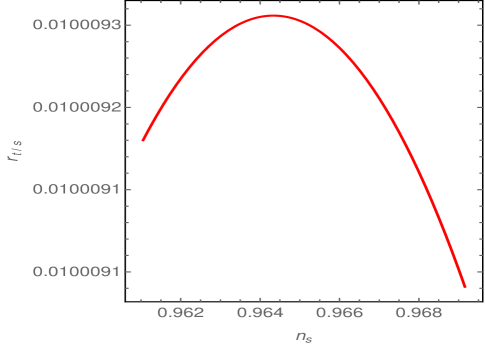
Figure 1: Parametric plot of $n_{s}$ vs $r_{\mathrm{t/s}}$ for $0.0155\leq\gamma\leq 0.0196$.

Now we are in a position to solve for the electromagnetic perturbation by using the solution of $\tilde{v}(k,\eta)$. By using the dimensionless variables $x=k\eta$, $\bar{A}_{\pm}(k,\eta)=\sqrt{k}A_{\pm}(k,\eta)$ and $V(k,\eta)=\sqrt{k}\tilde{v}(k,\eta)$, and using Eqs.(23) and (24), the electromagnetic equation (44) becomes,

$${\cal A}_{1}\frac{d^{2}\bar{A}_{\pm}}{dx^{2}}+{\cal A}_{2}\frac{d\bar{A}_{\pm}}{dx}\pm{\cal A}_{3}\bar{A}_{\pm}={\cal S}_{\pm},$$ (62)

where, the coefficients are,

$${\cal A}_{1} = \frac{1}{a_{f}^{2}}\bigg{(}\frac{k}{H}\bigg{)}^{4+m}+2(-1)^{m}x^{4+m}\leavevmode\nobreak\ \leavevmode\nobreak\ ;\leavevmode\nobreak\ \leavevmode\nobreak\ {\cal A}_{2}=-\frac{2}{x^{2}a_{f}^{2}}\bigg{(}\frac{k}{H}\bigg{)}^{4+m}+(4+2m)(-1)^{m}x^{3+m}$$ (63)

$${\cal A}_{3} = \frac{1}{a_{f}^{2}}\bigg{(}\frac{k}{H}\bigg{)}^{4+m}+2(-1)^{r}(2+r)\bigg{(}\frac{k}{H}\bigg{)}^{m-r}x^{3+r}-8s(-1)^{s}\bigg{(}\frac{k}{H}\bigg{)}^{m-s+2}x^{s+1}$$ (64)

$${\cal S}_{\pm} = \pm 2\sqrt{2}\bigg{(}\frac{h_{0}x^{5}}{H}\bigg{)}\bigg{(}\frac{k}{H}\bigg{)}^{m-1}\Bigg{[}(5+2\gamma)\bigg{(}\frac{dV}{dx}+\bigg{(}\frac{1+\gamma}{x}\bigg{)}V\bigg{)}+x\bigg{(}\frac{d^{2}V}{dx^{2}}-\frac{(2+3\gamma)}{x^{2}}V\bigg{)}\Bigg{]}.$$ (65)

Here it may be mentioned that due to the complicated nature, we solve the above equation numerically. For this we will consider values of $m$, $r$ and $s$ which lead to a scale invariant magnetic power spectrum in the superhorizon limit. For the modes lying outside the horizon, the scalar Mukhanov-Sasaki variable behaves as $\tilde{v}(k,\eta)\sim(-k\eta)^{-\nu+\frac{1}{2}}=(-k\eta)^{-1-\gamma}$ (see Eq.(53)), which indicates that $\tilde{v}(k,\eta)$ becomes proportional to $z(\eta)$ at the scale $-k\eta\rightarrow 0$. Furthermore the factor $\frac{k}{H}$ present in Eq.(62) is considered to be less than unity, which is indeed true for the CMB scale modes $\sim 10^{-40}\mathrm{GeV}^{-1}$ - the scale of interest to estimate the magnetic strength at the current universe. In account of these arguments, Eq.(62) in the superhorizon scale can be written as,

$$\frac{d^{2}\bar{A}_{\pm}}{dx^{2}} + \bigg{(}\frac{2+m}{x}\bigg{)}\frac{d\bar{A}_{\pm}}{dx}$$ (66)

$$\pm \left(-1\right)^{r-m}\left\{\left(\frac{k}{H}\right)^{m-r}\left(\frac{2+r}{x^{1+m-r}}\right)-4s\left(-1\right)^{-2-r}\left(\frac{k}{H}\right)^{2+m-s}\leavevmode\nobreak\ x^{3+m-s}\right\}\bar{A}_{\pm}=0$$

where, it may be observed that ${\cal S}_{\pm}$ vanishes due to the superhorizon solution of $\tilde{v}(k,\eta)$ given in Eq.(52). The above equation may not be solved analytically, thus we consider $m=r\geq s$ (later, we will show that such choices of parameters lead to the scale invariant electric as well as the scale invariant magnetic power spectrum). In effect, the term containing $\left(k/H\right)^{2+m-s}$ within the curly bracket becomes subdominant compared to the other one, since $k/H\ll 1$ for the CMB scale modes, in particular $k/H\sim 10^{-54}$ for $H\sim 10^{14}\mathrm{GeV}$. As a consequence, Eq.(66) turns out to be

$$\frac{d^{2}\bar{A}_{\pm}}{dx^{2}}+\bigg{(}\frac{2+m}{x}\bigg{)}\frac{d\bar{A}_{\pm}}{dx}\pm\bigg{(}\frac{2+m}{x}\bigg{)}\bar{A}_{\pm}=0$$ (67)

Eq.(67) has the following solution for $\bar{A}_{\pm}(k,\eta)$,

$$\bar{A}_{+}(k,\eta) = \big{(}-k\eta\big{)}^{\frac{1-m}{2}}\bigg{\{}C_{1}\mathrm{I}_{-m-1}\big{[}\sqrt{-(8+4m)x}\big{]}+D_{1}\mathrm{I}_{m+1}\big{[}\sqrt{-(8+4m)x}\big{]}\bigg{\}}$$ (68)

$$\bar{A}_{-}(k,\eta) = \big{(}-k\eta\big{)}^{\frac{1-m}{2}}\bigg{\{}C_{2}\mathrm{I}_{-m-1}\big{[}\sqrt{(8+4m)x}\big{]}+D_{2}\mathrm{I}_{m+1}\big{[}\sqrt{(8+4m)x}\big{]}\bigg{\}}$$ (69)

respectively, with $C_{1,2}$ and $D_{1,2}$ are integration constants. Here $\mathrm{I}_{n}(w)$ symbolizes the modified Bessel function of first kind having order $n$ and argument $w$, which, in the limit $w\ll 1$, has a power law form as $\mathrm{I}_{n}(w)=w^{n/2}$. Thus due to the presence of the modified Bessel function in Eq.(69), the term containing $C_{1}$ in the expression of $\bar{A}_{+}$ dominate over the other one containing $D_{1}$, i.e we may write $\lim_{|k\eta|\ll 1}\bar{A}_{+}\approx C_{1}(-k\eta)^{-m}$. Similar argument can also be drawn for $\bar{A}_{-}$, i.e $\lim_{|k\eta|\ll 1}\bar{A}_{-}\approx C_{2}(-k\eta)^{-m}$. As a result, Eq.(40) immediately leads to the electric and magnetic spectra in the superhorizon limit, as follows:

$$P^{(E)}(k,\eta) = \frac{m^{2}}{2\pi^{2}}\big{\{}|C_{1}|^{2}+|C_{2}|^{2}\big{\}}\bigg{[}f_{1}(\eta)+\frac{6f_{2}(\eta)}{a^{2}}\bigg{]}H^{4}\big{(}-k\eta\big{)}^{2-2m}$$

$$P^{(B)}(k,\eta) = \frac{f_{1}(\eta)}{2\pi^{2}}\big{\{}|C_{1}|^{2}+|C_{2}|^{2}\big{\}}H^{4}\big{(}-k\eta\big{)}^{4-2m}\leavevmode\nobreak\ \leavevmode\nobreak\ \leavevmode\nobreak\ .$$ (70)

Furthermore, as the two polarization modes evolves differently the magnetic field generated through this mechanism will be helical in nature and the helicity power spectrum during inflation comes as,

$$P^{(h)}(k,\eta) = \bigg{(}\frac{k^{3}}{2\pi^{2}a^{3}}\bigg{)}\big{(}-k\eta\big{)}^{-2m}\bigg{\{}\big{|}C_{1}\big{|}^{2}-\big{|}C_{2}\big{|}^{2}\bigg{\}}\leavevmode\nobreak\ \leavevmode\nobreak\ .$$ (71)

Specifically $(-k\eta)^{-2m}$ factor in the above expression clearly depicts that the comoving helicity spectra increases with time for a given mode for any positive value of $m$ during the inflationary era.
Eq.(70) points out that the scale dependence of the electric and the magnetic power spectra are different, in particular, $P^{(E)}\sim(-k\eta)^{2-2m}$ and $P^{(B)}\sim(-k\eta)^{4-2m}$. Thereby the electric power spectrum becomes scale invariant for $m=1$ while, in the magnetic case, $m=2$ leads to a scale invariant power spectrum. Thereby the coupling exponents consistent with a scale invariant magnetic power spectrum are constrained by, $m=2$, $r=2$ and $s\leq 2$; while for the scale invariant electric power spectrum, the corresponding constraint is given by $m=1$, $r=1$ and $s\leq 1$. Hence, in the following, we will solve the electromagnetic mode functions and will discuss the possible implications for the two different cases.

Here we would like to mention that in the Ratra like model where the EM Lagrangian is $\mathcal{L}_{em}=\sqrt{-g}f\left(\phi\right)F_{\mu\nu}F^{\mu\nu}$ with $f(\phi(\eta))=\left(a(\eta)/a_{f}\right)^{n}$, the magnetic and electric power spectra become scale invariant for $n=-6$ and $n=-4$ respectively Haque:2020bip ; Kobayashi:2019uqs . However, EFT framework provides us wider possibility of having such power spectrum. Assuming the canonical gauge kinetic term to be $f_{1}(\eta)=\left(a(\eta)/a_{f}\right)^{2}$, the other EFT coupling functions having exponents $m$, $r$, $s$ (as given in Eq.(24)), satisfying the condition $s\leq m=r=2$ can lead to a scale invariant magnetic spectrum, while $s\leq m=r=1$ will lead to scale invariant electric power spectrum. Therefore, the EFT coupling functions seem to play an important role in making the scale invariance of magnetic or electric power spectra in the present context.

Before we embark on estimating the magnetic field strength at large scale in the next section, we would like to address the strong coupling problem for general values of $m$, $r$ and $s$ in the spirit of EFT. For this purpose we need to start with the action of the EM and Dirac field, which in the present context, can be expressed by,

$$S_{em}+S_{\Psi} = \int d^{4}x\sqrt{-g}\bigg{[}-\frac{1}{4}f_{1}(\eta)F_{\mu\nu}F^{\mu\nu}+f_{2}(\eta)F^{0}_{i}F^{0i}+f_{3}(\eta)\epsilon^{ijk}F^{0}_{i}F_{jk}+f_{4}(\eta)\epsilon^{\mu\nu\alpha\beta}F_{\mu\nu}F_{\alpha\beta}\bigg{]}$$ (72)

$$+ \int d^{4}x\sqrt{-g}\bigg{[}\alpha(\eta)\bar{\Psi}\leavevmode\nobreak\ i\leavevmode\nobreak\ \gamma^{\mu}\mathbf{D}_{\mu}\Psi\leavevmode\nobreak\ +\leavevmode\nobreak\ \beta(\eta)\bar{\Psi}\leavevmode\nobreak\ i\leavevmode\nobreak\ \gamma^{0}\mathbf{D}_{0}\Psi\bigg{]}$$

where $\Psi$ is the Dirac field and $\mathbf{D}_{\mu}=\nabla_{\mu}-ieA_{\mu}$ is the covariant derivative. The part of the EM field in the above action has been considered earlier in Eq.(7), however in regard to the Dirac field, $S_{\Psi}$ contains two terms with EFT coefficients $\alpha(\eta)$ and $\beta(\eta)$. The underlying spatial diffeomorphism symmetry allows the coefficients $\alpha(\eta)$ and $\beta(\eta)$ to depend on $\eta$ only. Moreover the term $\beta(\eta)\bar{\Psi}i\gamma^{0}\mathbf{D}_{0}\Psi$ behaves as a scalar quantity under spatial diffeomorphism symmetry transformation and thus can be a possible term in $S_{\Psi}$ in the context of EFT of cosmology Tasinato:2014fia . By expanding the $S_{\Psi}$ in terms of temporal and spatial parts over the FRW spacetime, we get,

$$S_{\Psi}=\int d^{4}xa^{4}\bigg{[}i(\alpha(\eta)+\beta(\eta))\bar{\Psi}\gamma^{0}\mathbf{D}_{0}\Psi+i\alpha(\eta)\bar{\Psi}\gamma^{i}\mathbf{D}_{i}\Psi\bigg{]}$$ (73)

which makes Dirac field non-canonical. Therefore in order to make the Dirac field canonical, we redefine the field as,

$$\Psi\longrightarrow\widetilde{\Psi}=a^{2}\sqrt{\alpha(\eta)+\beta(\eta)}\leavevmode\nobreak\ \Psi\leavevmode\nobreak\ \leavevmode\nobreak\ .$$ (74)

Similarly due to the presence of the coupling functions $f_{i}(\eta)$ ($i=1,2,3,4$), the electromagnetic kinetic part becomes non-canonical, in particular,

$$S_{em}^{(kin)}=\frac{1}{2}\int d^{4}x\bigg{[}\left(f_{1}(\eta)+\frac{2f_{2}(\eta)}{a^{2}}\right)(A_{i}^{\prime})^{2}\bigg{]}\leavevmode\nobreak\ \leavevmode\nobreak\ .$$ (75)

Thus we redefine the EM field as,

$$A_{i}\longrightarrow\widetilde{A}_{i}=\left(f_{1}(\eta)+\frac{2f_{2}(\eta)}{a^{2}}\right)A_{i}$$ (76)

which in turn restores the canonicity of the EM field. In terms of such canonical variables, Eq.(72) immediately leads to the U(1) interaction between the EM and the Dirac fields as,

$$S_{int}=\int d^{4}x\bigg{[}\frac{e\leavevmode\nobreak\ \alpha(\eta)}{(\alpha(\eta)+\beta(\eta))\sqrt{f_{1}(\eta)+\frac{2f_{2}(\eta)}{a^{2}}}}\bigg{]}\bar{\widetilde{\Psi}}i\leavevmode\nobreak\ \gamma^{i}\widetilde{A}_{i}\widetilde{\Psi}=\int d^{4}x\leavevmode\nobreak\ \big{(}e\leavevmode\nobreak\ \lambda_{\mathrm{eff}}\big{)}\leavevmode\nobreak\ \bar{\widetilde{\Psi}}i\leavevmode\nobreak\ \gamma^{i}\widetilde{A}_{i}\widetilde{\Psi}$$ (77)

here $\lambda_{\mathrm{eff}}$ defines an effective electric charge as

$$e_{eff}=e\lambda_{\mathrm{eff}}=\frac{e}{{\left(1+\frac{\beta(\eta)}{\alpha(\eta)}\right)\sqrt{f_{1}(\eta)+\frac{2f_{2}(\eta)}{a^{2}}}}}$$ (78)

In order to avoid the strong coupling problem we need to have $\lambda_{\mathrm{eff}}\leqslant 1$ which leads to the following condition on the EFT parameters,

$$\left(1+\frac{\beta(\eta)}{\alpha(\eta)}\right)\geqslant\frac{1}{\sqrt{f_{1}(\eta)+\frac{2f_{2}(\eta)}{a^{2}}}}\leavevmode\nobreak\ \leavevmode\nobreak\ .$$ (79)

Thus, in the context of EFT magnetogenesis, the strong coupling problem can be naturally resolved provided the functions $a(\eta)$, $\beta(\eta)$, $f_{1}(\eta)$ and $f_{2}(\eta)$ satisfy Eq.(79) during inflation. In the present work, we consider $f_{1}(\eta)=\big{(}a/a_{\mathrm{f}}\big{)}^{2}$ and $f_{2}(\eta)=\big{(}a_{\mathrm{i}}/a\big{)}^{m}$ (see Eqs.(23) and (24)), due to which the above equation becomes,

$$\left(1+\frac{\beta(\eta)}{\alpha(\eta)}\right)\leavevmode\nobreak\ \geqslant\leavevmode\nobreak\ \frac{1}{\sqrt{\big{(}\frac{a}{a_{f}}\big{)}^{2}+\frac{2f_{2}}{a^{2}}\big{(}\frac{a_{i}}{a}\big{)}^{m}}}\leavevmode\nobreak\ \leavevmode\nobreak\ .$$ (80)

As mentioned earlier, we are interested in two distinct cases depending on whether the magnetic power spectrum or electric power spectrum becomes scale invariant, for which the corresponding parametric regime are given by $m=2$, $r=2$, $s\leq 2$ or $m=1$, $r=1$, $s\leq 1$. Thereby depending on such values of $m$ along with $a(\eta)=(-H\eta)^{-1}$, the functions $\alpha(\eta)$ and $\beta(\eta)$ can be chosen properly so that Eq.(80) holds true during inflation, which in turn leads to the resolution of the strong coupling problem.

5 Case-I: Scale invariant magnetic power spectrum

In this section, we consider the case where the magnetic power spectrum is scale invariant for the choices of the parameters $m=2$, $r=2$ and $s\leq 2$. Considering these set of parameter values we numerically solve Eq.(62) for $\bar{A}_{\pm}(k,\eta)$ which are depicted in Fig.2. During the numerical analysis, we take the Bunch-Davies initial condition for the electromagnetic mode functions and the initial conditions are set for the modes when they are well within the horizon length scale (i.e $-k\eta=10$). Moreover the numerical solutions are obtained upto the epoch when the modes are well outside the horizon ($-k\eta=10^{-4}$ has been used in our calculation).

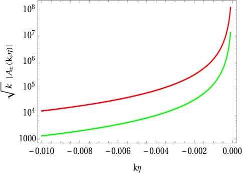
Figure 2: The red line represents $\sqrt{k}A_{+}(k,\eta)$ versus $k\eta$ and the green line represents $\sqrt{k}A_{-}(k,\eta)$ versus $k\eta$. Both the plots are for $k=0.05\mathrm{Mpc}^{-1}\approx 2\times 10^{-40}\mathrm{GeV}$, $H=10^{14}\mathrm{GeV}$ and $m=r=s=2$ respectively.

Fig.[2] clearly demonstrates that the $A_{+}$ mode dominates over the $A_{-}$ mode and thus the electromagnetic energy density in superhorizon limit is effectively determined by that of the contribution of $A_{+}$ mode.

5.1 Present magnetic strength and backreaction problem

In this section we will concentrate on the strength of the magnetic field in the present epoch. Conventionally one considers high electrical conductivity in the post inflationary epoch within the instantaneous reheating scenario, where inflaton makes a sudden jump from the inflationary phase to a radiation dominated phase. Due to large electrical conductivity electric field quickly vanishes and magnetic field freezes which will then adiabatically evolve till today in the form of large scale magnetic field. As we mentioned earlier for our analysis, coupling functions $f_{1}(\eta)=1$, $f_{2}(\eta)\approx f_{3}(\eta)\approx f_{4}(\eta)\approx h(\eta)\approx 0$, are assumed which will restore conformal symmetry and electromagnetic field follows the standard Maxwell’s equations. Hence, the frozen in magnetic field energy density evolves as $1/a^{4}$. The magnetic field strength at the present epoch is related with that at the end of inflation by the expression

$$\frac{\partial\rho(\vec{B})}{\partial\ln{k}}\bigg{|}_{0}=\bigg{(}\frac{a_{f}}{a_{0}}\bigg{)}^{4}\leavevmode\nobreak\ \frac{\partial\rho(\vec{B})}{\partial\ln{k}}\bigg{|}_{{\eta_{f}}},$$ (81)

where $\eta_{f}$ is the conformal time at the end of inflation and the suffix ’0’ denotes present time. With Eq.(40), the above equation yields the present magnetic strength ($B_{0}$)

$$B_{0}=\frac{1}{2\pi}\leavevmode\nobreak\ \bigg{\{}\sqrt{\big{|}\bar{A}_{+}(k,\eta_{f})\big{|}^{2}+\big{|}\bar{A}_{-}(k,\eta_{f})\big{|}^{2}}\bigg{\}}\bigg{(}\frac{a_{f}}{a_{0}}\bigg{)}^{2}\leavevmode\nobreak\ H^{2}\big{(}-k\eta_{f}\big{)}^{2},$$ (82)

where we recall that $\bar{A}_{\pm}=\sqrt{k}A_{\pm}$ and $k$ denotes the CMB scale ($\simeq 0.02\mathrm{Mpc}^{-1}$) at which we will estimate the current magnetic strength. In order to estimate $B_{0}$ from Eq.(82), we need to know $\frac{a_{0}}{a_{f}}$. The factor $\frac{a_{0}}{a_{f}}$ can be determined from the entropy conservation relation, i.e. from $gT^{3}a^{3}=\mathrm{constant}$, where $g$ is the effective relativistic degrees of freedom and $T$ denotes the temperature of the relativistic fluid, which finally yields $\frac{a_{0}}{a_{f}}\approx 10^{30}\big{(}H/10^{-5}M_{Pl}\big{)}^{1/2}$, with $H$ being the Hubble parameter during inflation and, in particular, we consider $H=10^{-5}M_{Pl}$. Moreover by using the numerical solution of $\bar{A}_{\pm}k,\eta)$ from Fig.[2], we get, $\bar{A}_{+}(k,\eta_{f})\simeq 10^{8}$ and $\bar{A}_{-}(k,\eta_{f})\simeq 10^{7}$ for $-k\eta_{f}=10^{-4}$. With such ingredients of $\frac{a_{0}}{a_{f}}$ and $\bar{A}_{\pm}k,\eta_{f})$, we estimate the magnetic strength at the present epoch from Eq.(82) to be

$$B_{0}\bigg{|}_{CMB}=0.82\times 10^{-13}\mathrm{G},$$ (83)

where we use the conversion $1\mathrm{G}=1.95\times 10^{-20}\mathrm{GeV}^{2}$. The above result gives us a typical value for the magnetic field at the present epoch in our present framework. It may be noticed that $B_{0}$ indeed depends on the inflationary Hubble parameter, in particular if we consider $H=10^{-6}M_{Pl}$, then $B_{0}$ will be estimated as $B_{0}\simeq 10^{-14}\mathrm{G}$ which, in comparison with Eq.(83), clearly argue that the current magnetic strength for $H=10^{-6}M_{Pl}$ gets 1 order lower than that of the case where $H=10^{-5}M_{Pl}$. However, from the observational Widrow:2002ud ; Kandus:2010nw ; Durrer:2013pga results a constraint on the current magnetic strength of $10^{-10}G\lesssim B_{0}\lesssim 10^{-22}G$ is obtained around the CMB scales. Therefore the theoretical prediction of $B_{0}$ lies within the observational constraints in the case where the magnetic power spectrum turns out to be scale invariant.
At this stage it deserves mentioning that the present case (i.e $m=2$), despite having compatibility with the observational strength of $B_{0}$, hinges with the backreaction problem. In particular, for $m=2$, we have from Eq.(70) $P^{(E)}(k,\eta)\propto(-k\eta)^{-2}$. In this case, as $-k\eta\rightarrow 0$ (i.e. towards the end of inflation), the electric energy density increases rapidly as $P^{(E)}\propto(-k\eta)^{-2}\rightarrow\infty$. Thereby the model runs into difficulties as the electric energy density would eventually exceed the inflaton energy density in the universe even before inflation ends.

Thus the scenario, where the magnetic power spectrum becomes scale invariant, can lead to required value of magnetic strength, however suffers from the backreaction problem. On contrary, the situation becomes different in the case where the electric power spectrum becomes scale invariant (i.e for $m=1$), as discussed in the following section.

6 Case-II: Scale invariant electric power spectrum

From Eq.(70) it is evident that the electric power spectrum becomes scale invariant for the parametric space satisfying $s\leq m=r=1$. Thereby considering a particular set of parameter values, in particular $m=r=s=1$, we solve the electromagnetic mode functions from Eq.(62) with the Bunch-Davies initial condition. However due to the complicated nature, Eq.(62) is solved numerically and they are depicted in Fig.[3]. The numerical analysis is performed for $k=0.05\mathrm{Mpc}^{-1}$ within the same same range $-10<k\eta<10^{-4}$ from sub to super Hubble scale.

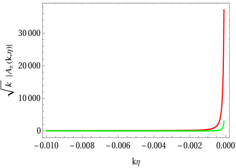
Figure 3: The red line represents $\sqrt{k}A_{+}(k,\eta)$ versus $k\eta$ and the green line represents $\sqrt{k}A_{-}(k,\eta)$ versus $k\eta$. Both the plots are for $k=0.05\mathrm{Mpc}^{-1}\approx 2\times 10^{-40}\mathrm{GeV}$, $H=10^{14}\mathrm{GeV}$ and $m=r=s=1$ respectively.

Fig.3 depicts that similar to the previous case, the $A_{+}$ mode is slightly dominated over the $A_{-}$ mode towards the end of inflation and thus the electromagnetic energy density in superhorizon limit is effectively determined by that of the contribution of $A_{+}$ mode. The solutions of $A_{\pm}$ immediately lead to the evolution of the helicity density during inflationary era. This is depicted in Fig.4 which clearly demonstrates that the comoving helicity density during inflation increases with time.

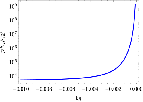
Figure 4: $P^{(h)}a^{3}/k^{3}$ versus $k\eta$ during inflationary epoch.

The scenario, where the electric power spectrum becomes scale invariant (i.e for $s\leq m=r=1$), leads to the electric and magnetic power spectra in the superhorizon scale as,

$$P^{(E)}(k,\eta) = \frac{m^{2}}{2\pi^{2}}H^{4}\big{\{}|C_{1}|^{2}+|C_{2}|^{2}\big{\}}\bigg{[}f_{1}(\eta)+\frac{6f_{2}(\eta)}{a^{2}}\bigg{]}$$

$$P^{(B)}(k,\eta) = \frac{f_{1}(\eta)}{2\pi^{2}}H^{4}\big{\{}|C_{1}|^{2}+|C_{2}|^{2}\big{\}}\big{(}-k\eta\big{)}^{2}\leavevmode\nobreak\ \leavevmode\nobreak\ \leavevmode\nobreak\ .$$ (84)

respectively, where we use Eq.(70). Thereby the spectral indices of the electric and magnetic spectra, defined by $n(E)=\frac{\partial\ln{P^{(E)}}}{\partial\ln{k}}$ and $n(B)=\frac{\partial\ln{P^{(B)}}}{\partial\ln{k}}$, become $n(E)=0$ and $n(B)=2$ respectively. It may be observed that in the scenario where the electric power spectrum becomes scale invariant, the spectral index for the magnetic power becomes positive, which in turn hints to the resolution of the backreaction problem. However, in order to investigate whether the backreaction of the electromagnetic field stays small during inflation, we shall first consider the energy stored in the electric field at a given time $\eta_{c}$, which is

$$\rho(\vec{E},\eta_{c})=\int_{k_{i}}^{k_{c}}\frac{\partial\rho(\vec{E})}{\partial\ln{k}}d\ln{k}=\frac{1}{2\pi^{2}}\bigg{[}e^{-2\big{(}N_{f}-N_{c}\big{)}}+6e^{-3N_{c}}\bigg{]}\big{\{}|C_{1}|^{2}+|C_{2}|^{2}\big{\}}H^{4}N_{c}\leavevmode\nobreak\ \leavevmode\nobreak\ ,$$ (85)

here $k_{i}$ and $k_{c}$ denote the modes that cross the horizon at the beginning of inflation and at $\eta=\eta_{c}$, respectively, and thus $k_{i}$ is considered to be the CMB scale. Moreover, $N_{f}$ is the total e-folding number of the inflation era. $N_{c}=\ln{\big{(}\frac{a_{c}}{a_{i}}\big{)}}$, with $a_{i}=a(\eta_{i})$ and $a_{c}=a(\eta_{c})$, is the e-fold number associated with conformal time $\eta=\eta_{c}$ during inflation. We also have the relation $|\eta_{c}|=k_{c}^{-1}$ and $k_{c}$ is obviously greater than the CMB mode momentum $k_{CMB}\approx 10^{-40}\mathrm{GeV}\approx 0.05\mathrm{Mpc}^{-1}$. Similarly, we determine the energy density coming from the magnetic fields, which yields

$$\rho(\vec{B},\eta_{c})=\int_{k_{i}}^{k_{c}}\frac{\partial\rho(\vec{B})}{\partial\ln{k}}d\ln{k}=\frac{1}{4\pi^{2}}e^{-2\big{(}N_{f}-N_{c}\big{)}}\big{\{}|C_{1}|^{2}+|C_{2}|^{2}\big{\}}H^{4}\bigg{(}1-e^{-2N_{c}}\bigg{)}\leavevmode\nobreak\ \leavevmode\nobreak\ .$$ (86)

To derive the above two expressions, we use the form of the coupling functions at $\eta=\eta_{c}$ in terms of the e-folding number, as $f_{1}(\eta_{c})=\big{(}a_{c}/a_{f}\big{)}^{2}=e^{-2\big{(}N_{f}-N_{c}\big{)}}$ and $f_{2}(\eta)=\big{(}a_{i}/a_{c}\big{)}=e^{-N_{c}}$. The total electromagnetic energy density at $\eta=\eta_{c}$ becomes

$$\rho_{em}(\eta_{c})=\rho(\vec{E},\eta_{c})+\rho(\vec{B},\eta_{c}) = \frac{1}{4\pi^{2}}\big{\{}|C_{1}|^{2}+|C_{2}|^{2}\big{\}}H^{4}\bigg{\{}N_{c}\left(2e^{-2\big{(}N_{f}-N_{c}\big{)}}+12e^{-3N_{c}}\right)$$ (87)

$$+ e^{-2\big{(}N_{f}-N_{c}\big{)}}\left(1-e^{-2N_{c}}\right)\bigg{\}}$$

where $C_{1,2}$ are integration constants as mentioned in Eq.(70). In order to avoid the backreaction issue, we have to ensure that the electromagnetic energy density is less than that of the background energy density. In particular, we have to show $\rho_{em}<3M_{Pl}^{2}H^{2}$ during inflation. The above expression, along with the consideration of $N_{c}\leq N_{f}\approx 60$, clearly indicate that the electromagnetic energy density during inflation is of the order of $H^{4}$, i.e.

$$\rho_{em}(\eta_{c})\sim H^{4}\leavevmode\nobreak\ \leavevmode\nobreak\ \leavevmode\nobreak\ .$$ (88)

The inflationary energy scale is less than the Planck scale; in particular, we consider $H=10^{-5}M_{Pl}$ and, thus, Eq.(88) leads to the inequality $\rho_{em}\ll M_{Pl}^{2}H^{2}$. This confirms that the electromagnetic field has a negligible backreaction on the background inflationary spacetime, leading to the resolution of the backreaction problem in the present magnetogenesis scenario.

6.1 Present magnetic strength

Following same methodology discussed for the scale invariant magnetic case (Sec.[5.1]), and using Eqs.(69) with $m=1$, the expression of the current magnetic strength turns out to be,

$$B_{0}=\frac{1}{2\pi}\leavevmode\nobreak\ \bigg{\{}\sqrt{\big{|}C_{1}\big{|}^{2}+\big{|}C_{2}\big{|}^{2}}\bigg{\}}\bigg{(}\frac{a_{f}}{a_{0}}\bigg{)}^{2}\leavevmode\nobreak\ H^{2}\big{(}-k\eta_{f}\big{)},$$ (89)

Here $C_{1,2}$ are integration constants appeared in Eq.(70) and $k$ symbolizes the momentum of the CMB scale $\approx 0.05\mathrm{Mpc}^{-1}$. As discussed earlier, by using the entropy conservation we get $\frac{a_{0}}{a_{f}}=10^{30}\big{(}H/10^{-5}M_{Pl}\big{)}^{1/2}$ with $H$ being the inflationary Hubble scale. Moreover in regard to $-k\eta_{f}$, we have the relation $|\eta_{f}|=\frac{1}{k_{f}}$ where $k_{f}$ is the mode which crosses the horizon at the end of inflation and thus $-k\eta_{f}$ is given by $-k\eta_{f}=\exp{\big{(}N_{f}\big{)}}$. With such expressions of $\frac{a_{0}}{a_{f}}$ and $-k\eta_{f}$, along with $H=10^{-5}M_{Pl}$, we estimate the magnetic strength at the present epoch from Eq.(89) to be,

$$B_{0}\bigg{|}_{CMB}\sim 10^{-40}\mathrm{G}$$ (90)

where we use $N_{f}=60$ and the conversion $1\mathrm{G}=1.95\times 10^{-20}\mathrm{GeV}^{2}$ may be useful. The above result provides an estimation for the magnetic field at the present epoch, as obtained from the framework. However, the observational results put a constraint on the current magnetic strength as $10^{-10}\mathrm{G}\lesssim B_{0}\lesssim 10^{-22}\mathrm{G}$ around the CMB scales. Therefore it is clear from Eq.(90) that the theoretical prediction of $B_{0}$ lies far below than the range of the observational expectation.

Thus as a whole, by comparing Secs.[5] and [6], it is evident that the scenario where the magnetic power spectrum is scale invariant (let, call it S1) gets distinct features in comparison to that of where the electric spectrum is scale invariant (let, call it S2). In particular, the scenario S1 is found to be observationally compatible with regard to the present magnetic strength, however suffers from the backreaction problem. On the other hand, the scenario S2 is indeed free from the backreaction problem, but does not predict sufficient magnetic field strength in present universe. Such distinctions of S1 and S2 are clearly depicted in Table[1]. However both the scenarios S1 and S2 are able to resolve the strong coupling problem as indicated earlier in Eq.(80).

Scenario	First feature	Second feature
S1 ($P^{(B)}$ is scale invariant)	Compatible with observation	Suffers from backreaction problem
S2 ($P^{(E)}$ is scale invariant)	Not compatible with observation	Free from backreaction problem

Table 1: Comparison between the scenarios S1 and S2

Above issues motivated us to look for physical solutions which can be theoretically as well as observationally viable concurrently. And for this we would consider the case when reheating play an important role. It deserves mentioning that our discussions on scenarios S1 and S2 are based on the fact that radiation domination starts immediately after the inflation ends which we call $instantaneous\leavevmode\nobreak\ reheating$ case. However a more physical approach would be if, during the cosmic evolution, the universe experiences a reheating phase with $non\leavevmode\nobreak\ zero$ e-fold number. In the following sections, we will discuss this possibility and its implications. We further assume that during reheating the conductivity will be vanishingly small as it is known that during entire period of reheating dynamics is mostly oscillating inflaton dominated. During the cosmological expansion of the universe, the EM field eventually evolves through the reheating phase and thus the electric and magnetic field(s) evolutions are considerably affected as compared to the instantaneous reheating case. As a consequence, there is a possibility that such an elongated reheating phase may make the models viable which we will investigate in Sec.[7]. However, our analysis shows that the presence of a reheating phase will not cure the difficulty of the scenario S1, because S1 suffers from the backreaction problem during inflation, which can not be rescued by a reheating phase that occurs after the inflation. Thus, in the following we will consider the scenario S2 with an elongated reheating phase and depending on the background reheating dynamics, two cases will arise – (i) when the reheating phase is characterized by the Kamionkowski like mechanism and (ii) where the reheating dynamics follow the perturbative mechanism.

7 Scenario with scale invariant electric field and reheating phase

The presence of a reheating phase with non-zero e-folding number considerably affects the magnetic field evolution in comparison to the instantaneous reheating case which we have considered in Sec.[6]. Actually in the instantaneous reheating scenario, the conductivity becomes huge after the end of inflation and as a consequence, the magnetic field evolves as $1/a^{4}$ from the end of inflation to the present epoch. However, if the reheating phase is considered to have a non-zero e-fold number (a natural consideration), then there is no reason to consider a large conductivity immediately after the inflation. In particular, the conductivity remains non-zero and small during the reheating epoch and consequently, the strong electric field induces the magnetic field Kobayashi:2019uqs . Due to such Faraday’s induction from electric to magnetic field, the redshift of the magnetic field becomes lesser as compared to $1/a^{4}$ in the reheating epoch, and thus the magnetic field’s present strength may become larger than what has been estimated in Eq.(90). Motivated by this situation, we aim to determine the magnetic field’s current strength in the present magnetogenesis model by considering the reheating phase to have a non-zero e-fold number.

To this end let us point out that extended reheating phase is known to effect the evolution of magnetic field at the background level Demozzi:2009fu ; Demozzi:2012wh . However importance of the Faraday effect during this phase has been critically explored recently in the context of magnetogenesis scenario Kobayashi:2019uqs ; Haque:2020bip ; Bamba:2020qdj . Furthermore, the effect of reheating is independent of our EFT construction which is only applied during inflation. Most important point is that accounting EM Faraday effect can put interesting constraints on the reheating parameters such as reheating temperature, inflaton equation of state, reheating e-folding number. Those constraints in turn will propagate into constraints on the EFT inflationary parameters in a model independent way. The constraints on the reheating and EFT inflationary parameters can be observed to be intertwined due to this reheating phase. We will discuss these in detail in the following sections.

7.1 Electromagnetic field evolution and the corresponding power spectrum during reheating

The effective theory parameters are so chosen, $f_{1}(\eta)=1$, $f_{2}(\eta)=f_{3}(\eta)=f_{4}(\eta)=h(\eta)=0$ that after the end of inflation the conformal symmetry coupling of the electromagnetic field (EM) is restored and, hence, the EM field evolution will follow the standard Maxwell’s equations in vacuum Kobayashi:2019uqs . In particular, the equations of motion of $A_{\pm}(k,\eta)$ are given by,

$$A_{\pm}^{\prime\prime(re)}(k,\eta)+k^{2}A_{\pm}^{(re)}(k,\eta)=0,$$ (91)

where $A_{\pm}^{(re)}(k,\eta)$ represents the electromagnetic mode function during reheating (i.e the superscript ’re’ denotes the reheating era). As a consequence of the restored conformal symmetry, the further quantum production of the gauge field stops during the reheating stage, in particular the absolute value of the Bogoliubov coefficient in the post-inflation becomes time independent. At this stage it deserves mentioning that we consider the universe to be a poor conductor, in particular the universe is considered to have a zero conductivity during the reheating era. However due to the Schwinger production, such consideration of zero conductivity needs an investigation, which, in the context of EFT, is expected to study in near future. Coming back to Eq.(91), the corresponding solution of the mode functions are,

$$A_{\pm}^{(re)}(k,\eta)=\frac{1}{\sqrt{2k}}\bigg{[}\alpha_{\pm}(k)\leavevmode\nobreak\ e^{-ik(\eta-\eta_{f})}+\beta_{\pm}(k)\leavevmode\nobreak\ e^{ik(\eta-\eta_{f})}\bigg{]},$$ (92)

with $\alpha_{\pm}(k)$, $\beta_{\pm}(k)$ being two integration constants and $\eta_{f}$ is the end instant of inflation. The integration constants can be determined by matching the EM mode functions and their derivative (with respect to the conformal time) at the junction of inflation-to-reheating; in particular,

$$A_{\pm}^{(re)}(k,\eta_{f})=A_{\pm}(k,\eta_{f})\leavevmode\nobreak\ \leavevmode\nobreak\ \leavevmode\nobreak\ \leavevmode\nobreak\ \leavevmode\nobreak\ \leavevmode\nobreak\ \leavevmode\nobreak\ \leavevmode\nobreak\ \leavevmode\nobreak\ \leavevmode\nobreak\ \leavevmode\nobreak\ \mathrm{and}\leavevmode\nobreak\ \leavevmode\nobreak\ \leavevmode\nobreak\ \leavevmode\nobreak\ \leavevmode\nobreak\ \leavevmode\nobreak\ \leavevmode\nobreak\ \leavevmode\nobreak\ \leavevmode\nobreak\ \leavevmode\nobreak\ \leavevmode\nobreak\ A_{\pm}^{\prime(re)}(k,\eta_{f})=A_{\pm}^{\prime}(k,\eta_{f}),$$ (93)

here $A_{\pm}(k,\eta)$ represents the mode function during inflation and follows Eq.(44) (note, the EM mode function during inflation is symbolized without any superscript, while the EM mode function during reheating is designated by the superscript ’re’). Eqs.(92) and (93) immediately lead to $\alpha_{\pm}(k)$ and $\beta_{\pm}(k)$ as,

$$\alpha_{\pm}(k) = \sqrt{\frac{k}{2}}\leavevmode\nobreak\ A_{\pm}(k,\eta_{f})+\frac{i}{\sqrt{2k}}\leavevmode\nobreak\ A_{\pm}^{\prime}(k,\eta_{f})$$

$$\beta_{\pm}(k) = \sqrt{\frac{k}{2}}\leavevmode\nobreak\ A_{\pm}(k,\eta_{f})-\frac{i}{\sqrt{2k}}\leavevmode\nobreak\ A_{\pm}^{\prime}(k,\eta_{f})$$ (94)

with $A_{\pm}(k,\eta_{f})$ can be obtained from their superhorizon solution as obtained in Eqs.(69) and (69), by putting $\eta=\eta_{f}$. If we think in terms of particle production during inflation, the above integration constants $\alpha_{\pm}(k)$ and $\beta_{\pm}(k)$ can be identified with the Bogoliubov coefficients at time $\eta=\eta_{f}$ for incoming and out going mode respectively. Naturally those remain constants during the subsequent evolution. $\big{|}\beta_{k}(\eta)\big{|}$ represents the total number of produced particles (having momentum $k$) at time $\eta_{f}$ from the Bunch-Davies vacuum defined at $\eta\rightarrow-\infty$. Hence, the time independency of the Bogoliubov coefficients during the reheating phase is a direct consequence of the fact that the conformal symmetry of the electromagnetic field is restored after inflation. Nonetheless, by plugging back the solution of $A_{\pm}^{(re)}(k,\eta)$ into Eq.(40) and by using the conformal invariance of the electromagnetic field (i.e $f_{1}(\eta)=1$, $f_{2}(\eta)=0$), we determine the magnetic and electric power spectra during the reheating epoch, as follows

$$\frac{\partial\rho(\vec{B})}{\partial\ln{k}} = \frac{1}{2\pi^{2}}\leavevmode\nobreak\ \sum_{r=\pm}\leavevmode\nobreak\ \frac{k^{5}}{a^{4}}\big{|}A_{r}^{(re)}(k,\eta)\big{|}^{2}$$ (95)

$$= \frac{1}{2\pi^{2}}\leavevmode\nobreak\ \sum_{r=\pm}\bigg{(}\frac{k^{4}}{a^{4}}\bigg{)}\bigg{[}|\alpha_{r}|^{2}+|\beta_{r}|^{2}+2|\alpha_{r}|\leavevmode\nobreak\ |\beta_{r}|\leavevmode\nobreak\ \cos{\big{\{}\theta^{(r)}_{1}-\theta^{(r)}_{2}-2k(\eta-\eta_{f})\big{\}}}\bigg{]}$$

$$\frac{\partial\rho(\vec{E})}{\partial\ln{k}} = \frac{1}{2\pi^{2}}\leavevmode\nobreak\ \sum_{r=\pm}\leavevmode\nobreak\ \frac{k^{2}}{a^{4}}\big{|}A_{r}^{\prime(re)}(k,\eta)\big{|}^{2}$$ (96)

$$= \frac{1}{2\pi^{2}}\leavevmode\nobreak\ \sum_{r=\pm}\bigg{(}\frac{k^{4}}{a^{4}}\bigg{)}\bigg{[}|\alpha_{r}|^{2}+|\beta_{r}|^{2}-2|\alpha_{r}|\leavevmode\nobreak\ |\beta_{r}|\leavevmode\nobreak\ \cos{\big{\{}\theta^{(r)}_{1}-\theta^{(r)}_{2}-2k(\eta-\eta_{f})\big{\}}}\bigg{]},$$

respectively, with $r$ being the electromagnetic polarization index and runs from $r=\pm$, and furthermore $\theta^{(r)}_{1}=\mathrm{Arg}[\alpha_{r}(k,\eta_{f})]$ and $\theta^{(r)}_{2}=\mathrm{Arg}[\beta_{r}(k,\eta_{f})]$. Consequently, the total electromagnetic power spectrum is

$$\frac{\partial\rho_{em}}{\partial\ln{k}}=\frac{\partial\rho(\vec{B})}{\partial\ln{k}}+\frac{\partial\rho(\vec{E})}{\partial\ln{k}}=\frac{1}{\pi^{2}}\leavevmode\nobreak\ \sum_{r=+,-}\leavevmode\nobreak\ \bigg{(}\frac{k^{4}}{a^{4}}\bigg{)}\bigg{[}\big{|}\alpha_{r}(k,\eta_{f})\big{|}^{2}+\big{|}\beta_{r}(k,\eta_{f})\big{|}^{2}\bigg{]}.$$ (97)

Furthermore, during the reheating epoch the helicity spectrum evolves as,

$$P^{(h)}(k,\eta) = \bigg{(}\frac{k^{3}}{\pi^{2}a^{3}}\bigg{)}\bigg{\{}\big{|}\beta_{+}\big{|}^{2}-\big{|}\beta_{-}\big{|}^{2}+\sqrt{1+\big{|}\beta_{+}\big{|}^{2}}\leavevmode\nobreak\ \big{|}\beta_{+}\big{|}\leavevmode\nobreak\ \cos{\big{\{}\theta^{(+)}_{1}-\theta^{(+)}_{2}-2k(\eta-\eta_{f})\big{\}}}$$ (98)

$$- \sqrt{1+\big{|}\beta_{-}\big{|}^{2}}\leavevmode\nobreak\ \big{|}\beta_{-}\big{|}\leavevmode\nobreak\ \cos{\big{\{}\theta^{(-)}_{1}-\theta^{(-)}_{2}-2k(\eta-\eta_{f})\big{\}}}\bigg{\}}\leavevmode\nobreak\ \leavevmode\nobreak\ ,$$

where we use $\big{|}\beta_{\pm}\big{|}^{2}-\big{|}\alpha_{\pm}\big{|}^{2}=1$. It can be observed from the above equations that individual electric and magnetic spectrum depends on the phase factor evolution which is the well known Faraday effect. However, the comoving total electromagnetic power spectrum is independent of time and behave as standard radiation field. Furthermore, due to zero electrical conductivity, the helicity spectrum also evolve with the phase factor during reheating. Moreover the relative phase factors between the Bogoliubov coefficients, from the numerical solutions of $A_{\pm}(k,\eta)$, are determined as,

$$\theta^{(+)}_{1}-\theta^{(+)}_{2} = \mathrm{Arg}\big{[}\alpha_{+}(\eta_{f})\beta_{+}^{*}(\eta_{f})\big{]}\simeq 3.141$$

$$\theta^{(-)}_{1}-\theta^{(-)}_{2} = \mathrm{Arg}\big{[}\alpha_{-}(\eta_{f})\beta_{-}^{*}(\eta_{f})\big{]}\simeq 3.141\leavevmode\nobreak\ \leavevmode\nobreak\ \leavevmode\nobreak\ .$$ (99)

This can also be understood from the analytic solutions of $A_{\pm}(k,\eta)$ in the superhorizon limit. In particular we obtained $\lim_{|k\eta|\ll 1}A_{\pm}\sim(-k\eta)^{-m}$ which leads to $\lim_{|k\eta|\ll 1}A^{\prime}_{\pm}\sim(-k\eta)^{-m-1}$. Therefore for $m=1$ (i.e the parametric value for the scenario S2), $A^{\prime}_{\pm}(k,\eta)$ dominates over the corresponding mode functions $A_{\pm}(k,\eta)$ at the limit $|k\eta|\rightarrow 0$ i.e towards the end of inflation. As a result,

$$\alpha_{\pm}(k,\eta_{f})\simeq\frac{i}{\sqrt{2k}}\leavevmode\nobreak\ A_{\pm}^{\prime}(k,\eta_{f})\leavevmode\nobreak\ \leavevmode\nobreak\ \leavevmode\nobreak\ \leavevmode\nobreak\ \leavevmode\nobreak\ \leavevmode\nobreak\ \leavevmode\nobreak\ \leavevmode\nobreak\ \leavevmode\nobreak\ \leavevmode\nobreak\ ,\leavevmode\nobreak\ \leavevmode\nobreak\ \leavevmode\nobreak\ \leavevmode\nobreak\ \leavevmode\nobreak\ \leavevmode\nobreak\ \leavevmode\nobreak\ \leavevmode\nobreak\ \leavevmode\nobreak\ \leavevmode\nobreak\ \beta_{\pm}(k,\eta_{f})\simeq\frac{-i}{\sqrt{2k}}\leavevmode\nobreak\ A_{\pm}^{\prime}(k,\eta_{f})\leavevmode\nobreak\ \leavevmode\nobreak\ \leavevmode\nobreak\ \leavevmode\nobreak\ .$$ (100)

The above expressions, due to the presence of the $\pm i$ factor, immediately lead to the relative phase between the respective Bogoliubov coefficients as $\theta_{1}^{(\pm)}-\theta_{2}^{(\pm)}=\pi$, which is in agreement with the numerical estimation in Eq.(99).

Now we need to know the unknown part of the phase factor “$\eta-\eta_{f}$” which is defined as

$$\eta-\eta_{f}=\int_{a_{f}}^{a}\frac{da}{a^{2}H}\leavevmode\nobreak\ \leavevmode\nobreak\ .$$ (101)

The presence of the Hubble parameter in Eq.(101) clearly indicates that in order to determine $\eta-\eta_{f}$ during the reheating phase, we need to state the background reheating dynamics, in particular how the inflaton energy density converts to other matter form. In the present context, we will consider two simple reheating mechanisms: (1) It is described by effective time independent equation of state and (2) perturbative reheating scenario.

7.2 Reheating with time independent equation of state: Evolution of Electromagnetic field

In regard to the reheating process, as the first consideration, we follow the conventional reheating mechanism proposed by Kamionkowski et al. Dai:2014jja , where the reheating phase is parametrized by a constant equation of state $\omega_{\mathrm{eff}}$. The reheating equation of state parameter (i.e $\omega_{\mathrm{eff}}$) remains constant during the entire reheating epoch and finally makes a sharp transition to the vale $1/3$ at the end of it, which in turn indicates the beginning of the radiation epoch. Due to the constant equation of state, the Hubble parameter during the reheating evolves as $H\propto a^{-\frac{3}{2}(1+\omega_{\mathrm{eff}})}$. Moreover, the reheating e-fold number $N_{\mathrm{re}}$, and the reheating temperature ($T_{\mathrm{re}}$) can be expressed in terms of the $\omega_{\mathrm{eff}}$ and of some inflationary parameters by the following relations Dai:2014jja ; Cook:2015vqa ,

$$N_{re}=\frac{4}{3\omega_{\mathrm{eff}}-1}\left[\frac{1}{4}ln(\rho_{f})-\frac{1}{4}ln\left(\frac{\pi^{2}g_{re}}{30}\right)-\frac{1}{3}\left(\frac{43}{11g_{s,re}}\right)-ln\left(\frac{a_{0}T_{0}}{k}\right)-ln(H_{*})+N_{f}\right]\leavevmode\nobreak\ \leavevmode\nobreak\ ,$$ (102)

$$T_{re}=\left(\frac{43}{11g_{s},re}\right)^{\frac{1}{3}}\bigg{(}\frac{a_{0}T_{0}}{k}\bigg{)}H_{*}e^{-N_{f}}e^{-N_{re}},$$ (103)

where, recall, the subscript ’*’ denotes the value of a quantity at the horizon crossing instant of CMB scale and $N_{f}$ is the e-fold number of the inflation epoch. Moreover $\rho_{f}$ denotes the inflaton energy density at the end of inflation. The present CMB temperature is taken as $T_{0}=2.725\mathrm{K}$, $k\approx 0.05\mathrm{Mpc}^{-1}$ is the pivot scale and $a_{0}$ denotes the present time scale factor. The symbols $g_{s,re}$ and $g_{re}$ represent the degrees of freedom for entropy at reheating and the effective number of relativistic species upon thermalization respectively, and moreover they are taken to be the same, particularly $g_{s,re}=g_{re}\approx 100$.
It may be observed from the above equations that both $N_{re}$ and $T_{re}$ depend on the inflationary parameters, in particular on $H_{*}$ and $N_{f}$. In regard to the inflationary quantities, we first consider the scalar spectral index ($n_{s}$) and the scalar perturbation amplitude ($\mathcal{A}_{s}$), which, in the context of EFT, take the following forms Cheung:2007st ,

$$n_{s}=1+\frac{4\dot{H}_{*}}{H_{*}^{2}}-\frac{\ddot{H}_{*}}{\dot{H}_{*}H_{*}}\leavevmode\nobreak\ \leavevmode\nobreak\ \leavevmode\nobreak\ \leavevmode\nobreak\ \leavevmode\nobreak\ \leavevmode\nobreak\ \leavevmode\nobreak\ \leavevmode\nobreak\ \leavevmode\nobreak\ ,\leavevmode\nobreak\ \leavevmode\nobreak\ \leavevmode\nobreak\ \leavevmode\nobreak\ \leavevmode\nobreak\ \leavevmode\nobreak\ \leavevmode\nobreak\ \leavevmode\nobreak\ \leavevmode\nobreak\ \mathcal{A}_{s}=\frac{H_{*}^{2}}{4\epsilon_{*}M_{Pl}^{2}}$$ (104)

with $\epsilon_{*}=-\dot{H}_{*}/H_{*}^{2}$ and an overdot represents the differentiation with respect to the cosmic time. The first and second derivatives of $H_{*}$ (appearing in the expression of $n_{s}$) are connected to the first and second slow roll parameters respectively. To determine $N_{f}$, we expand the Hubble parameter around $t=t_{*}$ (i.e the horizon crossing instant of the CMB scale) as follows,

$$H(t)=H_{*}+\dot{H}_{*}(t-t_{*})+\frac{1}{2}\ddot{H}_{*}(t-t_{*})^{2}$$ (105)

where we retain the terms upto $\mathcal{O}(\ddot{H}_{*})$, that means we consider upto the second slow roll parameter. If the duration of inflation is designated by $\Delta t$, then the Hubble parameter at the end of inflation ($H_{f}$) is given by,

$$H_{f}=H_{*}+\dot{H}_{*}\Delta t+\frac{1}{2}\ddot{H}_{*}\big{(}\Delta t\big{)}^{2}\leavevmode\nobreak\ \leavevmode\nobreak\ .$$ (106)

Inverting the above equation, we get the duration of inflation in terms of $H_{*}$, $H_{f}$, $\dot{H}_{*}$ and $\ddot{H}_{*}$ as,

$$\Delta t=\frac{|\dot{H}_{*}|}{\ddot{H}_{*}}\left(1-\sqrt{1-\frac{2\ddot{H}_{*}}{|\dot{H}_{*}|^{2}}(H_{*}-H_{f})}\right)$$ (107)

with $|\dot{H}_{*}|=-\dot{H}_{*}$. Using the above expressions, we determine the inflationary e-folding number and is given by,

$$N_{f} = \int_{t_{*}}^{t_{f}}H(t)dt$$ (108)

$$= \frac{H_{*}|\dot{H}_{*}|}{\ddot{H}_{*}}\left(1-\sqrt{1-\frac{2\ddot{H}_{*}}{|\dot{H}_{*}|^{2}}(H_{*}-H_{f})}\right)-\frac{|\dot{H}_{*}|^{3}}{2\ddot{H}_{*}^{2}}\left(1-\sqrt{1-\frac{2\ddot{H}_{*}}{|\dot{H}_{*}|^{2}}(H_{*}-H_{f})}\right)^{2}$$

$$+ \frac{|\dot{H}_{*}|^{3}}{6\ddot{H}_{*}^{2}}\left(1-\sqrt{1-\frac{2\ddot{H}_{*}}{|\dot{H}_{*}|^{2}}(H_{*}-H_{f})}\right)^{3}$$

where, in the second line, we use the expression of $\Delta t$ from Eq.(107). Furthermore, Eq.(104) leads to $\dot{H}_{*}$ and $\ddot{H}_{*}$ in terms of $n_{s}$, $\mathcal{A}_{s}$ as follows

$$|\dot{H}_{*}|=\frac{H_{*}^{4}}{4\mathcal{A}_{s}M^{2}_{Pl}}\leavevmode\nobreak\ \leavevmode\nobreak\ \leavevmode\nobreak\ \leavevmode\nobreak\ \leavevmode\nobreak\ \leavevmode\nobreak\ \leavevmode\nobreak\ \leavevmode\nobreak\ \leavevmode\nobreak\ \leavevmode\nobreak\ ,\leavevmode\nobreak\ \leavevmode\nobreak\ \leavevmode\nobreak\ \leavevmode\nobreak\ \leavevmode\nobreak\ \leavevmode\nobreak\ \leavevmode\nobreak\ \leavevmode\nobreak\ \leavevmode\nobreak\ \leavevmode\nobreak\ \leavevmode\nobreak\ \leavevmode\nobreak\ \leavevmode\nobreak\ \ddot{H}_{*}=\frac{H_{*}^{5}}{4\mathcal{A}_{s}M^{2}_{Pl}}\left(\frac{H_{*}^{2}}{\mathcal{A}_{s}M^{2}_{Pl}}-(1-n_{s})\right)$$ (109)

respectively. Here we would like to mention that, as depicted in Fig.[1], the observable quantities like scalar spectral index and tensor to scalar ratio are indeed compatible with the Planck constraints in the present EFT context where the EFT coefficients satisfy Eq.(48). Thereby using the viable value(s) of $n_{s}$ and $\mathcal{A}_{s}$, in particular we will consider $n_{s}=0.9649$ and $\ln{[10^{10}\mathcal{A}_{s}]}=3.044$ (i.e the central values of $n_{s}$ and $\mathcal{A}_{s}$ in respect to the Planck constraints), one can determine $\dot{H}_{*}$ and $\ddot{H}_{*}$ from Eq.(109), which in turn will evaluate the inflationary e-fold number from Eq.(108).
Coming back to the quantity $\eta-\eta_{f}$, we first consider the behaviour of the Hubble parameter during the reheating stage. Due to the fact that the effective EoS remains constant, the Hubble parameter behaves as $H\propto a^{-\frac{3}{2}(1+\omega_{\mathrm{eff}})}$, and as a result, the term $\eta-\eta_{f}$ boils down to the following simple form:

$$\eta-\eta_{f}=\frac{2}{\big{(}1+3\omega_{\mathrm{eff}}\big{)}}\bigg{[}\frac{1}{aH}-\frac{1}{a_{f}H_{f}}\bigg{]},$$ (110)

where we use Eq.(101). Due to the above expression of $\eta-\eta_{f}$ along with the fact that $\big{|}\beta_{\pm}(\eta_{f})\big{|}^{2}\gg 1$, the magnetic power spectrum during the reheating era becomes Kobayashi:2019uqs

$$\frac{\partial\rho(\vec{B})}{\partial\ln{k}}=\frac{1}{\pi^{2}}\bigg{(}\frac{k^{4}}{a^{4}}\bigg{)}\leavevmode\nobreak\ \sum_{r=+,-}\leavevmode\nobreak\ \big{|}\beta_{r}\big{|}^{2}\leavevmode\nobreak\ \bigg{\{}\mathrm{Arg}\big{[}\alpha_{r}\leavevmode\nobreak\ \beta_{r}^{*}\big{]}-\pi-\bigg{(}\frac{4k}{3\omega_{\mathrm{eff}}+1}\bigg{)}\bigg{(}\frac{1}{aH}-\frac{1}{a_{f}H_{f}}\bigg{)}\bigg{\}}^{2}.$$ (111)

The above equation clearly indicates that the magnetic power evolution during reheating scales by two different terms: (1) the conventinal one that goes as $1/a^{4}$ and (2) the term that redshifts as $\propto a^{-6}H^{-2}$, emerging from $\frac{1}{aH}$ in the right hand side of Eq.(111). Due to the reason that the universe undergoes through deceleration, the EoS follows $\omega_{\mathrm{eff}}>-\frac{1}{3}$, and thus the magnetic power effectively scales by the component $\propto a^{-6}H^{-2}$. In the context of instantaneous reheating, the magnetic power evolves as $a^{-4}$ from end of inflation until today, where as if one considers intermediate reheating phase with negligible conductivity the evolution of magnetic power will be as described above. Due to this fact present strength of the magnetic field can be lager compared to that for the instantaneous reheating case. This particular phenomena can make S2-like magnetogenesis scenario viable which we will elaborate next. The electric power in the reheating epoch goes evolves as,

$$\frac{\partial\rho(\vec{E})}{\partial\ln{k}}=\frac{1}{\pi^{2}}\bigg{(}\frac{k^{4}}{a^{4}}\bigg{)}\leavevmode\nobreak\ \sum_{r=+,-}\leavevmode\nobreak\ \big{|}\beta_{r}(\eta_{f})\big{|}^{2}$$ (112)

Hence the electric power evolve exactly like radiation during reheating at large scale. Finally the behaviour of the helicity spectrum takes the following form in the large $|\beta(k,\eta_{f})|$ limit,

$$P^{(h)}=\bigg{(}\frac{k^{3}}{\pi^{2}a^{3}}\bigg{)}\bigg{\{}\big{|}\beta_{+}(k,\eta_{f})\big{|}^{2}-\big{|}\beta_{-}(k,\eta_{f})\big{|}^{2}\bigg{\}}\bigg{\{}\frac{4k}{3\omega_{\mathrm{eff}}+1}\bigg{(}\frac{1}{aH}-\frac{1}{a_{f}H_{f}}\bigg{)}\bigg{\}}^{2}\propto\frac{1}{a^{5}H^{2}}+\cdots\leavevmode\nobreak\ \leavevmode\nobreak\ .$$ (113)

During reheating the Hubble parameters behaves as $H=a^{-\frac{3}{2}(1+\omega_{\mathrm{eff}})}$. Hence, from Eq.(113), the leading behaviour of the helicity density will be, $a^{3}P^{(h)}\sim a^{1+3\omega_{\mathrm{eff}}}$. For all reheating equation of state $\omega_{\mathrm{eff}}>-\frac{1}{3}$, the comoving helicity during the reheating era monotonically grows with time.

7.2.1 Present day magnetic field and constraints on reheating parameters, $\omega_{eff}$

Here we may recall that the scenario S2 with an instantaneous reheating mechanism does not predict a sufficient magnetic strength in the present epoch, in particular it predicts $B_{0}=10^{-40}\mathrm{G}$ as shown in Eq.(90). Given the characteristic difference in evolution of magnetic power spectrum during reheating, we see how those models can be made viable with the CMB observations. With this motivation in mind we are now in position to constrain such model with respect to the observation. For this let us first express the Hubble parameter at the end of reheating ($H_{re}$) in terms of that of the end of inflation ($H_{f}$) as

$$H_{re}=H_{f}\bigg{(}\frac{a_{re}}{a_{f}}\bigg{)}^{-\frac{3}{2}(1+\omega_{eff})},$$ (114)

where the suffix ’re’ denotes the end point of reheating and the scale factor $a_{re}$ can be identified as ${a_{re}}/{a_{f}}=e^{N_{\mathrm{re}}}$ with $N_{\mathrm{re}}$ being the e-fold number of the reheating epoch and given in Eq.(102). Consequently, from Eq.(111) we evaluate the magnetic power spectrum at the end instant of reheating, as

$$\frac{\partial\rho(\vec{B})}{\partial\ln{k}}\bigg{|}_{re}=\bigg{(}\frac{k^{4}}{a_{re}^{4}\pi^{2}}\bigg{)}\sum_{r=\pm}\leavevmode\nobreak\ \big{|}\beta_{r}\big{|}^{2}\leavevmode\nobreak\ \bigg{\{}\mathrm{Arg}\big{[}\alpha_{r}\beta_{r}^{*}\big{]}-\pi-\bigg{(}\frac{4k}{(3\omega_{\mathrm{eff}}+1)a_{f}H_{f}}\bigg{)}\bigg{[}\bigg{(}\frac{H_{f}}{H_{re}}\bigg{)}^{\delta}-1\bigg{]}\bigg{\}}^{2}\leavevmode\nobreak\ \leavevmode\nobreak\ \leavevmode\nobreak\ ,$$ (115)

where, $\delta=(3\omega_{\mathrm{eff}}+1)/(3\omega_{\mathrm{eff}}+3)$. After the reheating era the conductivity of the universe is assumed to be sufficiently large, so that, the electric field dies out very fast. Therefore, Faraday induction will halt. Consequently the magnetic field begins to evolve according to radiation as $a^{-4}$ till today. The present-day magnetic power spectrum then becomes,

$$\frac{\partial\rho(\vec{B})}{\partial\ln{k}}\bigg{|}_{0}=\bigg{(}\frac{a_{re}}{a_{0}}\bigg{)}^{4}\leavevmode\nobreak\ \frac{\partial\rho(\vec{B})}{\partial\ln{k}}\bigg{|}_{{re}}$$ (116)

and, as a result, Eq.(115) leads to the current magnetic strength, as

$$B_{0}=\frac{\sqrt{2}}{\pi}\bigg{(}\frac{k}{a_{0}}\bigg{)}^{2}\sqrt{\sum_{r=\pm}\big{|}\beta_{r}\big{|}^{2}\leavevmode\nobreak\ \bigg{\{}\mathrm{Arg}\big{[}\alpha_{r}\beta_{r}^{*}\big{]}-\pi-\bigg{(}\frac{4}{3\omega_{\mathrm{eff}}+1}\bigg{)}\bigg{(}\frac{k}{a_{f}H_{f}}\bigg{)}\bigg{[}\bigg{(}\frac{H_{f}}{H_{re}}\bigg{)}^{\delta}-1\bigg{]}\bigg{\}}^{2}}\leavevmode\nobreak\ \leavevmode\nobreak\ \leavevmode\nobreak\ ,$$ (117)

The above expression clearly indicates that the magnetic field’s current amplitude explicitly depends on the reheating parameters $(\omega_{\mathrm{eff}},H_{re}$), and inflationary $n_{s}$. As a consequence, probing $B_{0}$ and its nature opens up a new window to look into the reheating phase. Given an inflationary model, the expression in Eq.(117) establishes the connection between the current magnetic strength $B_{0}$ and the reheating EoS parameter $\omega_{\mathrm{eff}}$. Thus we may argue that the effective equation of state is no longer a free parameter, rather it is fixed by the $B_{0}$ via CMB.

Having obtained the final expression of $B_{0}$, now we confront our model with the CMB observations which put a constraint on the current magnetic strength, as $10^{-10}\mathrm{G}\lesssim B_{0}\lesssim 10^{-22}\mathrm{G}$ Widrow:2002ud ; Kandus:2010nw ; Durrer:2013pga . For this purpose, we need ${H_{f}}/{H_{re}}$, which depends on $N_{\mathrm{re}}$, as discussed after Eq.(114). In our effective theory framework, we have three main input parameters, the inflationary energy scale $H^{*}$ and the inflationary e-folding number $N_{f}$, and the reheating equation of state $\omega_{eff}$. All the other parameters can be computed such as $N_{\mathrm{re}},H_{f},\dot{H}_{*}$ and $\ddot{H}_{*}$. Given the observed central values $n_{s}=0.9649$, $\ln{\big{[}10^{10}\mathcal{A}_{s}\big{]}=3.044}$, for our estimation we consider two different sets of values for $(H_{*},N_{f})$ particular, we consider - (1) $(H_{*},N_{f})=(10^{-5}M_{Pl},50)$ and (2) $(H_{*},N_{f})=(10^{-5}M_{Pl},55)$. The first and second sets correspond to the Hubble parameter at the end of inflation as $H_{f}=3.61\times 10^{-6}M_{Pl}$ and $H_{f}=1.62\times 10^{-6}M_{Pl}$ respectively, i.e $H_{f}$ decreases with increasing e-folding number, as expected. With such considerations, we plot $B_{0}$ versus $\omega_{\mathrm{eff}}$ by using Eq.(117) in Fig.5.

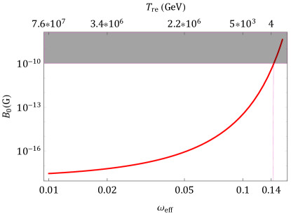
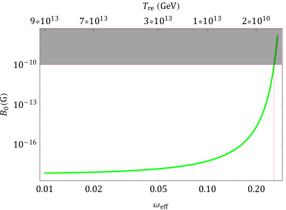
Figure 5: $B_{0}$ (in Gauss units) vs $\omega_{\mathrm{eff}}$ with $k=0.05\mathrm{Mpc}^{-1}$ in the Kamionkowski like reheating scenario. The reheating temperature for different values of $\omega_{\mathrm{eff}}$ is shown in the upper label of the $x$-axis. In the left plot: $H_{*}=10^{-5}M_{Pl}$, $n_{s}=0.9649$, $\ln{\big{[}10^{10}\mathcal{A}_{s}\big{]}=3.044}$, $N_{f}=50$ and in the right plot: $H_{*}=10^{-5}M_{Pl}$, $n_{s}=0.9649$, $\ln{\big{[}10^{10}\mathcal{A}_{s}\big{]}=3.044}$, $N_{f}=55$.

It clearly demonstrates that the theoretical prediction of $B_{0}$ lies well within the observational constraints for a certain range of values of the reheating EoS parameter, given by : $0.01\lesssim\omega_{\mathrm{eff}}\lesssim 0.14$ for $N_{f}=50$ and $0.01\lesssim\omega_{\mathrm{eff}}\lesssim 0.25$ for $N_{f}=55$, which are also consistent with BBN constraint on the minimum reheating temperature $\sim 10^{-2}\mathrm{GeV}$.

Finally let us also point out the how the helical nature of the magnetic field spectrum evolves which is shown in the Fig.[6]. The figure depicts that the comoving helicity density grows with time during the reheating stage. However, during the post reheating phase, the universe is considered to be a very good conductor, which in turn makes the electromagnetic mode functions constant over time. As a result, the helicity goes as $1/a^{3}$ or equivalently the comoving helicity becomes constant during the after reheating phase to the present epoch. Important to realize that introduction of reheating has increased the comoving helicity density by manifold compared to that the helicity density produced for the instantaneous reheating case.

Figure 6: $P^{(h)}a^{3}/k^{3}$ versus $k/(aH)$ during and after reheating era. The reheating EoS is taken as $\omega_{\mathrm{eff}}=0$ for which $\frac{k}{aH}\propto k\sqrt{a}\propto k\eta$.

7.3 Perturbative reheating with time dependent EoS: Evolution of magnetic field

In this section we consider perturbative reheating scenario Maity:2018dgy , where the inflaton energy density ($\rho_{\mathrm{\phi}}$) decays into the radiation energy density ($\rho_{\mathrm{R}}$) governed by the Boltzmann equations Eqs.(119) and (120). This essentially leads to the time dependent effective equation of state (EoS) during phase, which is defined by

$$\omega_{\mathrm{eff}}=\frac{3\omega_{\phi}\rho_{\phi}+\rho_{R}}{3\big{(}\rho_{\phi}+\rho_{R}\big{)}}.$$ (118)

Where, $\omega_{\phi}$ symbolizes the time averaged EoS of the inflaton field. For example during reheating, for oscillating canonical inflaton with potential $V(\phi)\propto\phi^{p}$, assumes the time averaged EoS, $\omega_{\mathrm{\phi}}={(p-2)}/{(p+2)}$. However, effective equation of state $\omega_{eff}$ naturally Maity:2018dgy depend on time. Initially, $\omega_{\mathrm{eff}}$ behaves as approximately equal to $\omega_{\phi}$, and after a certain instance of time it smoothly transits to the value $\approx 1/3$ setting the beginning of the radiation epoch. This scenario is different from that of the earlier one where the inflaton energy density is assumed to be instantaneously converted into radiation energy density at the end of reheating.

The set of Boltzmann equations governing the evolution of $\rho_{\phi}$ and $\rho_{R}$ are given by,

$$\frac{d\Phi}{d\xi}+\frac{\sqrt{3}M_{Pl}\Gamma_{\phi}}{H^{2}_{f}}(1+\omega_{\phi})\frac{\xi^{1/2}\Phi}{\Phi\xi^{-3\omega_{\phi}}+R\xi^{-1}}=0$$ (119)

and

$$\frac{dR}{d\xi}-\frac{\sqrt{3}M_{Pl}\Gamma_{\phi}}{H^{2}_{f}}(1+\omega_{\phi})\frac{\xi^{\frac{3(1-2\omega_{\phi}}{2}}\Phi}{\Phi\xi^{-3\omega_{\phi}}+R\xi^{-1}}=0\leavevmode\nobreak\ \leavevmode\nobreak\ \leavevmode\nobreak\ ,$$ (120)

respectively. The Boltzmann equations are expressed in terms of a rescaled scale factor $\xi(a)=a/a_{f}$ for convenience, with $a_{f}$ being the scale factor at the end of inflation. Furthermore $\Gamma_{\mathrm{\phi}}$ symbolizes the decay rate from inflaton to radiation energy density and the comoving densities are rescaled in terms of the dimensionless variable as,

$$\Phi=\bigg{(}\frac{\rho_{\phi}}{H_{\mathrm{f}}^{4}}\bigg{)}\xi^{3\big{(}1+\omega_{\phi}\big{)}}\leavevmode\nobreak\ \leavevmode\nobreak\ \leavevmode\nobreak\ \leavevmode\nobreak\ \leavevmode\nobreak\ \leavevmode\nobreak\ ;\leavevmode\nobreak\ \leavevmode\nobreak\ \leavevmode\nobreak\ \leavevmode\nobreak\ \leavevmode\nobreak\ \leavevmode\nobreak\ \leavevmode\nobreak\ \leavevmode\nobreak\ R=\bigg{(}\frac{\rho_{R}}{H_{\mathrm{f}}^{4}}\bigg{)}\xi^{4}\leavevmode\nobreak\ \leavevmode\nobreak\ .$$ (121)

For solving the above Boltzmann equations, the natural initial conditions will be set at the end of inflation as follows,

$$\Phi(\xi=1)=\rho_{f}/H_{f}^{4}\leavevmode\nobreak\ \leavevmode\nobreak\ \leavevmode\nobreak\ \leavevmode\nobreak\ \leavevmode\nobreak\ \leavevmode\nobreak\ \mathrm{and}\leavevmode\nobreak\ \leavevmode\nobreak\ \leavevmode\nobreak\ \leavevmode\nobreak\ \leavevmode\nobreak\ \leavevmode\nobreak\ R(\xi=1)=0\leavevmode\nobreak\ ,$$ (122)

$\rho_{f}$ is the inflaton energy density at $\xi=1$. Furthermore, the reheating temperature is identified from the radiation temperature $T_{\mathrm{rad}}$ at the point of $H(t_{\mathrm{re}})=\Gamma_{\mathrm{\phi}}$ ($t_{\mathrm{re}}$ denotes the end of reheating), when maximum inflaton energy density transfer into radiation.

$$T_{re}=T_{rad}^{end}=\left(\frac{30}{\pi^{2}g_{re}}\right)^{1/4}\big{[}\rho_{R}(\Gamma_{\phi},\xi_{re},n_{s})\big{]}^{1/4}\leavevmode\nobreak\ .$$ (123)

with $\xi_{re}$ being the rescaled factor at the end of reheating i.e $\xi_{re}=a_{re}/a_{f}$. From the entropy conservation of thermal radiation, the relation among $T_{\mathrm{rad}}=T_{\mathrm{re}}$ at equilibrium, and $(T_{0},T_{\nu 0}=(4/11)^{1/3}T_{0})$, temperature of the CMB photon and neutrino background at the present day respectively, can be written as

$$g_{re}T_{re}^{3}=\left(\frac{a_{0}}{a_{re}}\right)^{3}\left(2T_{0}^{3}+6\frac{7}{8}T_{\nu 0}^{3}\right).$$ (124)

Using above equation, one arrives at the following well known relation

$$T_{re}=\left(\frac{43}{11g_{re}}\right)^{\frac{1}{3}}\left(\frac{a_{0}T_{0}}{k}\right)H_{*}e^{-N_{\mathrm{f}}}e^{-N_{\mathrm{re}}}\leavevmode\nobreak\ \leavevmode\nobreak\ ,$$ (125)

where $N_{re}$ is the e-folding number of the reheating era. To establish one to one correspondence between $T_{\mathrm{re}}$ and $\Gamma_{\mathrm{\phi}}$, we combine the equations (123) and (125). To fixed the values of decay width $\Gamma_{\mathrm{\phi}}$ in terms of spectral index ($n_{s}$), we use one further condition at the end of the reheating

$$H^{2}(\xi_{re})=\frac{1}{\xi_{\mathrm{re}}^{2}}\bigg{(}\frac{d\xi_{\mathrm{re}}}{dt}\bigg{)}^{2}=\frac{\rho_{\mathrm{\phi}}(\Gamma_{\mathrm{\phi}},\xi_{\mathrm{re}},n_{s})+\rho_{R}(\Gamma_{\phi},\xi_{re},n_{s}))}{3M_{\mathrm{Pl}}^{2}}=\Gamma_{\mathrm{\phi}}^{2}\leavevmode\nobreak\ \leavevmode\nobreak\ .$$ (126)

With the above equipments, we solve the Hubble parameter ($H^{2}(\xi)=\frac{1}{3M_{Pl}^{2}}\big{(}\rho_{\phi}+\rho_{R}\big{)}$) numerically along with the coupled Boltzmann differential equations (119) and (120). The numerical solutions of $H(\xi)$ is depicted in Fig.[7] which corresponds to a particular set: $T_{\mathrm{re}}=10^{6}\mathrm{GeV}$ and $\omega_{\phi}=0$ respectively.

Figure 7: The background Hubble parameter $H(\xi)$ versus $\xi$ during the reheating era i.e for $1\leq\xi\leq\xi_{re}$. The plot corresponds to $\omega_{\phi}=0$ and $T_{\mathrm{re}}=10^{6}\mathrm{GeV}$.

In the perturbative reheating scenario, the quantity $\eta-\eta_{f}$ of Eq.(101) can be expressed as,

$$\eta-\eta_{f}=\bigg{(}\frac{1}{a_{f}H_{\mathrm{f}}}\bigg{)}\int_{1}^{\xi}\frac{d\xi}{\xi^{2}}\frac{\sqrt{3}M_{Pl}H_{\mathrm{f}}}{\sqrt{\rho_{r}(\xi)+\rho_{\phi}(\xi)}}\leavevmode\nobreak\ \leavevmode\nobreak\ ,$$ (127)

where $\rho_{\phi}$ and $\rho_{R}$ are governed by the coupled Eqs.(119) and (120). Due to the complicated nature of the Boltzmann equations, the integral in Eq.(127) may not be performed in a closed form, however we will perform it numerically for various values of $\omega_{\phi}$. The above expression of $\eta-\eta_{f}$ immediately leads to the magnetic power spectrum during the reheating era as follows,

$$\frac{\partial\rho(\vec{B})}{\partial\ln{k}}=\frac{1}{\pi^{2}}\bigg{(}\frac{k^{4}}{a^{4}}\bigg{)}\leavevmode\nobreak\ \sum_{r=\pm}\leavevmode\nobreak\ \big{|}\beta_{r}\big{|}^{2}\leavevmode\nobreak\ \bigg{\{}\mathrm{Arg}\big{[}\alpha_{r}\beta_{r}^{*}\big{]}-\pi-2\bigg{(}\frac{k}{a_{f}H_{\mathrm{f}}}\bigg{)}\int_{1}^{\xi}\frac{d\xi}{\xi^{2}}\frac{\sqrt{3}M_{Pl}H_{\mathrm{f}}}{\sqrt{\rho_{r}(\xi)+\rho_{\phi}(\xi)}}\bigg{\}}^{2}.$$ (128)

Furthermore, due to the fact that $\big{|}\beta_{r}(\eta_{f})\big{|}\gg 1^{2}$, the electric power spectrum during the reheating phase goes as,

$$\frac{\partial\rho(\vec{E})}{\partial\ln{k}}=\frac{1}{\pi^{2}}\bigg{(}\frac{k^{4}}{a^{4}}\bigg{)}\leavevmode\nobreak\ \sum_{r=\pm}\leavevmode\nobreak\ \big{|}\beta_{r}(\eta_{f})\big{|}^{2}\leavevmode\nobreak\ \leavevmode\nobreak\ .$$ (129)

The above expressions will be used in investigating whether the scenario S2 with a reheating phase, characterized by perturbative mechanism, will predict sufficient magnetic strength at present universe. We will analyze this for different values of $\omega_{\phi}$ in Sec.[7.3.1], which in turn will help to probe various informations of the reheating phase.

7.3.1 Present day magnetic field and constraints on perturbative reheating

Following this same methodology considered for the earlier reheating scenario, we will see hos perturbative reheating dynamics is constrained by the present value of the magnetic field. During the perturbative reheating the effective EoS $\omega_{\mathrm{eff}}$ time dependent. However, to set constrain, we may introduce an average effective EoS defined by,

$$\langle{\omega}_{\mathrm{eff}}\rangle=\frac{1}{\xi_{re}-1}\int_{1}^{\xi_{re}}\omega_{\mathrm{eff}}\leavevmode\nobreak\ d\xi=\frac{1}{\xi_{re}-1}\int_{1}^{\xi_{re}}\bigg{\{}\frac{3\omega_{\phi}\rho_{\phi}+\rho_{R}}{3\big{(}\rho_{\phi}+\rho_{R}\big{)}}\bigg{\}}d\xi$$ (130)

where we use Eq.(118) and recall, $\xi=1$ to $\xi=\xi_{re}$ denotes the reheating phase. It may be observed from Eq.(130) that $\langle{\omega}_{\mathrm{eff}}\rangle$ contains the information of background evolution of $\rho_{\phi}$ and $\rho_{R}$, and also depends on the inflaton EoS ($\omega_{\phi}$). Following Eq.(128), and the detailed procedure discussed in the previous section, one obtains the magnetic field strength at present epoch as,

$$B_{0}=\frac{\sqrt{2}}{\pi}\bigg{(}\frac{k}{a_{0}}\bigg{)}^{2}\sqrt{\sum_{r=\pm}\big{|}\beta_{r}\big{|}^{2}\leavevmode\nobreak\ \bigg{\{}\mathrm{Arg}\big{[}\alpha_{r}\leavevmode\nobreak\ \beta_{r}^{*}\big{]}-\pi-\bigg{(}\frac{2kM_{pl}}{a_{f}H_{\mathrm{f}}}\bigg{)}\int_{1}^{\xi_{re}}\frac{d\xi}{\xi^{2}}\frac{\sqrt{3}H_{\mathrm{f}}}{\sqrt{\rho_{r}(\xi)+\rho_{\phi}(\xi)}}\bigg{\}}^{2}}$$ (131)

For this purpose, we will take same set of parameter values as before for our numerical computation, $(H_{*},N_{f})=(10^{-5}M_{Pl},50)$ and (2) $(H_{*},N_{f})=(10^{-5}M_{Pl},55)$. Given those values we first need to evaluate $\xi_{re}$ appearing in the upper limit of the integral, which is done by simultaneously satisfying the following equations:

$$H(\xi_{re})=\Gamma_{\phi}\leavevmode\nobreak\ \leavevmode\nobreak\ ,\leavevmode\nobreak\ \leavevmode\nobreak\ T_{re}=\left(\frac{30}{\pi^{2}g_{re}}\right)^{1/4}\rho_{R}^{1/4}\leavevmode\nobreak\ \leavevmode\nobreak\ ,\leavevmode\nobreak\ \leavevmode\nobreak\ T_{re}=\left(\frac{43}{11g_{s},re}\right)^{\frac{1}{3}}\frac{a_{0}T_{0}}{k}H_{*}e^{-N_{f}}e^{-N_{re}}$$ (132)

Using $\xi_{re}$ and the numerical solutions of $\rho_{\phi}$ and $\rho_{R}$ from the Boltzmann equations, we get the variation of $B_{0}$ with $\omega_{\phi}$, which is depicted in Fig.8. It is with respect to the average effective EoS of the reheating era, i.e in respect to $\langle\omega_{\mathrm{eff}}\rangle$ defined in Eq.(130).

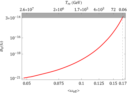
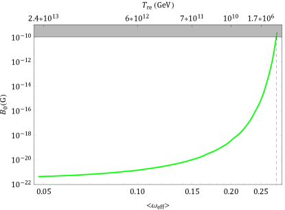
Figure 8: $B_{0}$ (in Gauss units) vs $\langle\omega_{\mathrm{eff}}\rangle$ with $k=0.05\mathrm{Mpc}^{-1}$ in the perturbative reheating scenario. The reheating temperature for different values of $\langle\omega_{\mathrm{eff}}\rangle$ is shown in the upper label of the $x$-axis. In the left plot: $H_{*}=10^{-5}M_{Pl}$, $n_{s}=0.9649$, $\ln{\big{[}10^{10}\mathcal{A}_{s}\big{]}=3.044}$, $N_{f}=50$ and in the right plot: $H_{*}=10^{-5}M_{Pl}$, $n_{s}=0.9649$, $\ln{\big{[}10^{10}\mathcal{A}_{s}\big{]}=3.044}$, $N_{f}=55$.

As we may observe that similar to the earlier reheating case, the current magnetic strength in the perturbative reheating mechanism increases with the average effective EoS (i.e $\langle\omega_{\mathrm{eff}}\rangle$, defined in Eq.(130)) and lies within the observational constraints for suitable regime of reheating parameters. However the viable range of the reheating parameters differ in the two reheating mechanisms respectively. In particular, the compatibility of the scenario S2, with a reheating phase characterized by perturbative mechanism, both with the CMB observations on $B_{0}$ and with the BBN constraint on the reheating temperature leads to a constraint on $\langle\omega_{\mathrm{eff}}\rangle$ as: $0.05\lesssim\langle\omega_{\mathrm{eff}}\rangle\lesssim 0.17$ for $N_{f}=50$ and $0.04\lesssim\langle\omega_{\mathrm{eff}}\rangle\lesssim 0.27$ for $N_{f}=55$ respectively.

8 Conclusion

Effective field theory is a powerful tool in various branches of physics. In the present work we studied in detail inflationary magnetogenesis in this EFT framework. In the cosmological universe, four dimensional diffeomorphism symmetry is generically broken down to spatial diffeomorphism. Using this remaining symmetry we have written down most general action upto quadratic order in scalar, tensor, electromagnetic vector fluctuation. In this framework, electromagnetic sector automatically breaks conformal invariance which plays the crucial role in producing the gauge field from the quantum vacuum. We have also considered the parity broken term which further gives rise the helical magnetic has great observational significance. The form of the coupling functions have been considered in such a way that during inflation electromagnetic field evolves non-trivially, however, at late times (in particular after the end of inflation), the conformal symmetry of the EM field is restored and consequently the standard Maxwellian evolution is restored.

We have explored the evolution of the EM, scalar and tensor perturbation, and determine the primordial power spectrum taking into account PLANCK, and Large scale magnetic field observation. In regard to the cosmological evolution of the electric and magnetic fields, we discussed possibilities of scale invariant magnetic or electric power spectrum particularly at the superhorizon scale. If we consider instantaneous reheating after the inflation, it is observed that the scale invariant magnetic field scenario is observationally compatible, however, suffers from the backreaction problem. On the other hand, scale invariant electric field scenario is indeed free from the backreaction problem, but does not predict sufficient amount of magnetic strength in the present universe.

To cure this problem, we next introduce reheating phase with non-trivial evolution dynamics with non-zero e-folding number. Two different reheating mechanisms are considered: (i) Reheating dynamics is Dai:2014jja governed by a time independent effective equation of state ($\omega_{\mathrm{eff}}$). (ii) As a second possibility, we consider perturbative reheating scenario where effective equation of state is time evolving due to non-trivial decay of inflaton into the radiation. Because of reheating phase post-inflation dynamics of EM field becomes non-trivial. Most interesting case arises when one considers vanishing electrical conductivity during this phase, which induces additional magnetic field from non-vanishing electric field due to well known Faraday effect. However, after the end of reheating, this effect ceases to exist as universe becomes good conductor and, hence, the electric field vanishes. Specifically, the magnetic field energy density evolves as $a^{-6}H^{-2}$ during the reheating era, and after the reheating, as $a^{-4}$. Furthermore, we observed that reheating also helps increase the helicity of the magnetic field if parity violation is introduced in the system as shown in the Fig.6. Reheating phase, therefore, helps enhancing the present value of magnetic field as compared to ordinary instantaneous reheating case. Our detail analysis shows that this is precisely the mechanism which can provide right magnitude of the present magnetic field for the scale invariant electric field scenario. However, this mechanism does not help to cure the problem for the scale invariant magnetic case. The reason being that the backreaction problem occurs during the inflation and thus can not be rescued by any post inflationary phase. We will discuss the possible resolution of this problem in our forthcoming paper.

Most importantly, introducing reheating era not only helps to obtain the right magnitude of the large scale magnetic field, it allows one to obtain valuable information about the reheating EoS parameter ($\omega_{\mathrm{eff}}$) which in turn can potentially constraint the inflationary model itself, which has been discussed before in some of our recent works Bamba:2020qdj ; Haque:2020bip . Therefore, probing large scale magnetic field opens up a new probe to look into the reheating phase which is otherwise very difficult to constrain. Combining CMB, presently observed constraint on $B_{0}$ and the BBN constraint, our analysis restrict the value of of $\omega_{\mathrm{eff}}$ as follows: (i) $0.01\lesssim\omega_{\mathrm{eff}}\lesssim 0.14$ for $N_{f}=50$ and $0.01\lesssim\omega_{\mathrm{eff}}\lesssim 0.25$ for $N_{f}=55$ for the reheating scenario where EoS is constant. and (ii) $0.05\lesssim\langle\omega_{\mathrm{eff}}\rangle\lesssim 0.17$ for $N_{f}=50$ and $0.04\lesssim\langle\omega_{\mathrm{eff}}\rangle\lesssim 0.27$ for $N_{f}=55$ for the perturbative reheating scenario (recall, $N_{f}$ is the inflationary e-folding number and $\langle\omega_{\mathrm{eff}}\rangle$ is the average effective EoS during the reheating era defined in Eq.(130)). This provides a viable constraint on the reheating EoS parameter from CMB observations.

Appendix A Discussion on several magnetogenesis models and their equivalence with the EFT formalism

As we have already mentioned in Sec.2 that in this magnetogenesis scenario we can find one to one correspondence between the EFT approach and several well established models of inflationary magnetogenesis, here in this section we discuss that various magnetogenesis models can be embedded within the electromagnetic action (7) for suitable forms of the EFT coupling parameters $f_{i}(\eta)$. For example,

• The model where the EM field couples with a scalar field (generally the inflaton field), in particular the action is given by,

  $$S_{m1}=\int d^{4}x\sqrt{-g}\left[f(\phi)F_{\mu\nu}F^{\mu\nu}\right]$$ (133)

  where $\phi$ is the scalar field under consideration and $f(\phi)$ is the conformal breaking coupling function. The above magnetogenesis model without (i.e instantaneous reheating) or with reheating phase have been explored earlier in Demozzi:2009fu ; Haque:2020bip ; Kobayashi:2019uqs where the coupling function is taken as $f(\phi(\eta))=\left(a(\eta)/a_{f}\right)^{n}$, with $\phi=\phi(\eta)$ being determined by the background evolution of the scalar field and $a(\eta)$ is the scale factor of the FRW metric. The possible implications of an elongated reheating phase have been discussed in such magnetogenesis scenario, and moreover the parameter $n$ is constrained for which the model predicts sufficient magnetic strength and also becomes free from various problems like the backreaction issue, the strong coupling problem etc Demozzi:2009fu ; Haque:2020bip ; Kobayashi:2019uqs .
  Most importantly, the action (133) has a direct correspondence with the EFT action given in Eq.(7) when the EFT parameters get the following forms:

  $$f_{1}(\eta)=\left(\frac{a(\eta)}{a_{f}}\right)^{n}\leavevmode\nobreak\ \leavevmode\nobreak\ \leavevmode\nobreak\ \leavevmode\nobreak\ \leavevmode\nobreak\ \leavevmode\nobreak\ ,\leavevmode\nobreak\ \leavevmode\nobreak\ \leavevmode\nobreak\ \leavevmode\nobreak\ \leavevmode\nobreak\ f_{2}(\eta)=f_{3}(\eta)=f_{4}(\eta)=0$$ (134)

  respectively.

• On contrary to the scalar field coupled magnetogenesis model, let us consider the model where the EM field couples with the background spacetime curvature, in particular with the Ricci scalar as well as with the Gauss-Bonnet scalar curvature. The corresponding action is Bamba:2020qdj ,

  $$S_{m2}=\int d^{4}x\sqrt{-g}\left[-\frac{1}{4}F_{\mu\nu}F^{\mu\nu}+f(R,\mathcal{G})F_{\mu\nu}F^{\mu\nu}\right]$$ (135)

  where the coupling function $f(R,\mathcal{G})$ spoils the conformal invariance of the EM field and has the form as $f(R,\mathcal{G})=\kappa^{2q}\left(R^{q}+\mathcal{G}^{q/2}\right)$, with $q$ being the model parameter. This magnetogenesis model without (i.e instantaneous reheating) and with reheating phase have been explored in Bamba:2020qdj where an elongated reheating phase seems to have a considerable impact on the magnetic field evolution, and in turn it predicts sufficient magnetic strength for suitable range of the reheating EoS. Moreover the above form of $f(R,\mathcal{G})$ does not lead to scale invariant magnetic or electric power spectrum for the possible values of $q$.
  Once again, the action $S_{m2}$ can be embedded within the EFT action (7), provided the EFT parameters are considered to have the following forms,

  $$f_{1}(\eta) = -\frac{1}{4}+\kappa^{2q}\left(R^{q}+\mathcal{G}^{q/2}\right)$$

  $$f_{2}(\eta) = f_{3}(\eta)=f_{4}(\eta)=0$$ (136)

  respectively, where $R(\eta)=\frac{6}{a^{2}}\left(\mathcal{H}^{\prime}+\mathcal{H}^{2}\right)$ and $\mathcal{G}(\eta)=\frac{24}{a^{4}}\mathcal{H}^{2}\mathcal{H}^{\prime}$, with $\mathcal{H}$ represents the conformal Hubble parameter in the FRW metric.

• In both the above magnetogenesis models, the equivalent EFT parameters like $f_{3}(\eta)$ and $f_{4}(\eta)$ become zero, mainly due to the absence of the parity violating terms in the EM field Lagrangian. However, on contrary, we can consider certain magnetogenesis models where the parity violating terms are indeed present in the EM Lagrangian and the equivalent $f_{3}(\eta)$ or $f_{4}(\eta)$ (or both) are non-zero. One of such models is explored by the authors of Kushwaha:2020nfa , where the EM field is considered to couple with the background Riemann tensor, particularly the action is,

  $$S_{m3}=\int d^{4}x\sqrt{-g}\left[-\frac{1}{4}F_{\mu\nu}F^{\mu\nu}-\frac{\sigma}{M^{2}}\tilde{R}^{\mu\nu\alpha\beta}F_{\mu\nu}F_{\alpha\beta}\right]$$ (137)

  where $\sigma$ is a model parameter, $R_{\rho\sigma}^{\alpha\beta}$ is the Riemann tensor and its dual is $\tilde{R}^{\mu\nu\alpha\beta}=\frac{1}{2}\epsilon^{\mu\nu\rho\sigma}R_{\rho\sigma}^{\alpha\beta}$. Due to the presence of the dual tensor in the Lagrangian, the two polarization modes of the EM field evolve differently, which in turn leads to the generation of helical magnetic field. The non-minimal coupling of the EM field to the Riemann tensor generates sufficient primordial helical magnetic fields at large scales, and the model is also free from the backreaction, strong coupling problems.
  In the case of background FRW spacetime (with $a(\eta)$ being the scale factor), the action $S_{m3}$ turns out to be,

  $$S_{m3}=\int d^{4}x\sqrt{-g}\left[-\frac{1}{4}F_{\mu\nu}F^{\mu\nu}+\frac{\sigma}{2M^{2}}\left(\frac{a^{\prime 2}}{a^{2}}+\frac{a^{\prime\prime}}{a}\right)\epsilon^{ijk}F^{0}_{i}F_{jk}\right]\leavevmode\nobreak\ \leavevmode\nobreak\ .$$ (138)

  Thereby interestingly, the $S_{m3}$ can be thought as equivalent with the EFT action given in Eq.(7) if the the EFT parameters have the forms like,

  $$f_{1}(\eta) = -\frac{1}{4}\leavevmode\nobreak\ \leavevmode\nobreak\ \leavevmode\nobreak\ \leavevmode\nobreak\ \leavevmode\nobreak\ \leavevmode\nobreak\ \leavevmode\nobreak\ \leavevmode\nobreak\ \leavevmode\nobreak\ \leavevmode\nobreak\ ,\leavevmode\nobreak\ \leavevmode\nobreak\ \leavevmode\nobreak\ \leavevmode\nobreak\ \leavevmode\nobreak\ \leavevmode\nobreak\ \leavevmode\nobreak\ \leavevmode\nobreak\ \leavevmode\nobreak\ \leavevmode\nobreak\ \leavevmode\nobreak\ f_{2}(\eta)=0\leavevmode\nobreak\ \leavevmode\nobreak\ ,$$

  $$f_{3}(\eta) = \frac{\sigma}{2M^{2}}\left(\frac{a^{\prime 2}}{a^{2}}+\frac{a^{\prime\prime}}{a}\right)\leavevmode\nobreak\ \leavevmode\nobreak\ \leavevmode\nobreak\ \leavevmode\nobreak\ ,\leavevmode\nobreak\ \leavevmode\nobreak\ \leavevmode\nobreak\ \leavevmode\nobreak\ f_{4}(\eta)=0$$ (139)

  respectively. Here it may be mentioned that in Kushwaha:2020nfa , the authors considered an $instantaneous\leavevmode\nobreak\ reheating$ mechanism in regard to the magnetogenesis model (137), however one may expect that the inclusion of a reheating phase with non-zero e-fold number will enhance the magnetic strength at present epoch compared to the instantaneous reheating case.

• As a well known one, we consider the Turner-Widrow model Turner:1987bw where the action is given by,

  $$S_{m4}=\int d^{4}x\sqrt{-g}\left[-\frac{1}{4}F_{\mu\nu}F^{\mu\nu}+\frac{1}{12}RA^{2}\right]$$ (140)

  where $R$ is the background Ricci scalar. The presence of the effective potential term for the vector field (i.e $V\left(A_{\mu}A^{\mu}\right)$) in the above action spoils the U(1) invariance of the electromagnetic field, due to which the massive vector field gets three physical degrees of freedom: two of them are usual transverse modes and the other one is the longitudinal mode. The longitudinal mode with momentum $p^{2}>R/6$ appears as a ghost field in the model, i.e a field with negative kinetic energy Himmetoglu:2009qi ; Himmetoglu:2008zp ; Himmetoglu:2008hx ; Karciauskas:2010as . However on contrary, in the present work, it is the kinetic term of the electromagnetic field that gets coupled through the EFT parameters, and hence there is no potential term of the electromagnetic field appearing in the action. Thus the U(1) invariance is preserved in the present model, and consequently the longitudinal mode is absent. This clearly indicates that the action $S_{m4}$ is not equivalent with the EFT action (7) considered in this work.

References

- (1) D. Grasso and H. R. Rubinstein, Phys. Rept. 348 (2001), 163-266 [arXiv:astro-ph/0009061 [astro-ph]].
- (2) R. Beck, Space Sci. Rev. 99 (2001), 243-260 [arXiv:astro-ph/0012402 [astro-ph]].
- (3) L. M. Widrow, Rev. Mod. Phys. 74 (2002), 775-823 [arXiv:astro-ph/0207240 [astro-ph]].
- (4) A. Kandus, K. E. Kunze and C. G. Tsagas, Phys. Rept. 505 (2011), 1-58 [arXiv:1007.3891 [astro-ph.CO]].
- (5) R. Durrer and A. Neronov, Astron. Astrophys. Rev. 21 (2013), 62 [arXiv:1303.7121 [astro-ph.CO]].
- (6) K. Subramanian, Rept. Prog. Phys. 79 (2016) no.7, 076901 [arXiv:1504.02311 [astro-ph.CO]].
- (7) L. Biermann, Z. Naturforsch. 5a, 65 (1950)
- (8) R. M. Kulsrud and E. G. Zweibel, Rept. Prog. Phys. 71 (2008), 0046091 [arXiv:0707.2783 [astro-ph]].
- (9) A. Brandenburg and K. Subramanian, Phys. Rept. 417 (2005), 1-209 [arXiv:astro-ph/0405052 [astro-ph]].
- (10) K. Subramanian, Astron. Nachr. 331 (2010), 110-120 [arXiv:0911.4771 [astro-ph.CO]].
- (11) R. Sharma, S. Jagannathan, T. R. Seshadri and K. Subramanian, Phys. Rev. D 96 (2017) no.8, 083511 [arXiv:1708.08119 [astro-ph.CO]].
- (12) R. Sharma, K. Subramanian and T. R. Seshadri, Phys. Rev. D 97 (2018) no.8, 083503 [arXiv:1802.04847 [astro-ph.CO]].
- (13) R. K. Jain and M. S. Sloth, Phys. Rev. D 86 (2012), 123528 [arXiv:1207.4187 [astro-ph.CO]].
- (14) R. Durrer, L. Hollenstein and R. K. Jain, JCAP 03 (2011), 037 [arXiv:1005.5322 [astro-ph.CO]].
- (15) S. Kanno, J. Soda and M. a. Watanabe, JCAP 12 (2009), 009 [arXiv:0908.3509 [astro-ph.CO]].
- (16) L. Campanelli, Int. J. Mod. Phys. D 18 (2009), 1395-1411 [arXiv:0805.0575 [astro-ph]].
- (17) V. Demozzi, V. Mukhanov and H. Rubinstein, JCAP 08 (2009), 025 [arXiv:0907.1030 [astro-ph.CO]].
- (18) V. Demozzi and C. Ringeval, JCAP 05, 009 (2012) [arXiv:1202.3022 [astro-ph.CO]].
- (19) K. Bamba and S. D. Odintsov, JCAP 0804 (2008) 024 [arXiv:0801.0954 [astro-ph]].
- (20) K. Bamba, S. Nojiri and S. D. Odintsov, Phys. Rev. D 77, 123532 (2008) [arXiv:0803.3384 [hep-th]].
- (21) K. Bamba, C. Q. Geng and L. W. Luo, JCAP 1210, 058 (2012) [arXiv:1208.0665 [astro-ph.CO]].
- (22) K. Bamba and M. Sasaki, JCAP 02 (2007), 030 [arXiv:astro-ph/0611701 [astro-ph]].
- (23) K. Bamba and J. Yokoyama, Phys. Rev. D 69 (2004), 043507 [arXiv:astro-ph/0310824 [astro-ph]].
- (24) K. Bamba and J. Yokoyama, Phys. Rev. D 70 (2004), 083508 [arXiv:hep-ph/0409237 [hep-ph]].
- (25) K. Bamba, E. Elizalde, S. D. Odintsov and T. Paul, [arXiv:2012.12742 [gr-qc]] (JCAP accepted).
- (26) M. R. Haque, D. Maity and S. Pal, [arXiv:2012.10859 [hep-th]].
- (27) M. Giovannini, [arXiv:2012.14720 [gr-qc]].
- (28) M. Giovannini, Class. Quant. Grav. 35 (2018) no.8, 084003 doi:10.1088/1361-6382/aab17d [arXiv:1712.07598 [astro-ph.CO]].
- (29) M. Giovannini, Int. J. Mod. Phys. D 13 (2004), 391-502 doi:10.1142/S0218271804004530 [arXiv:astro-ph/0312614 [astro-ph]].
- (30) T. Kobayashi and M. S. Sloth, Phys. Rev. D 100 (2019) no.2, 023524 [arXiv:1903.02561 [astro-ph.CO]].
- (31) B. Ratra, Astrophys. J. Lett. 391 (1992), L1-L4
- (32) P. A. R. Ade et al. [Planck], Astron. Astrophys. 594 (2016), A19 [arXiv:1502.01594 [astro-ph.CO]].
- (33) D. Chowdhury, L. Sriramkumar and M. Kamionkowski, JCAP 10 (2018), 031 [arXiv:1807.07477 [astro-ph.CO]].
- (34) T. Vachaspati, Phys. Lett. B 265 (1991), 258-261
- (35) M. S. Turner and L. M. Widrow, Phys. Rev. D 37 (1988), 2743
- (36) K. Takahashi, K. Ichiki, H. Ohno and H. Hanayama, Phys. Rev. Lett. 95 (2005), 121301 [arXiv:astro-ph/0502283 [astro-ph]].
- (37) I. Agullo and J. Navarro-Salas, [arXiv:1309.3435 [gr-qc]].
- (38) R. J. Z. Ferreira, R. K. Jain and M. S. Sloth, JCAP 10 (2013), 004 [arXiv:1305.7151 [astro-ph.CO]].
- (39) K. Atmjeet, T. R. Seshadri and K. Subramanian, Phys. Rev. D 91 (2015), 103006 [arXiv:1409.6840 [astro-ph.CO]].
- (40) A. Kushwaha and S. Shankaranarayanan, Phys. Rev. D 102 (2020) no.10, 103528 doi:10.1103/PhysRevD.102.103528 [arXiv:2008.10825 [gr-qc]].
- (41) R. Sharma, [arXiv:2102.09358 [astro-ph.CO]].
- (42) P. Adshead, J. T. Giblin, T. R. Scully and E. I. Sfakianakis, JCAP 12 (2015), 034 [arXiv:1502.06506 [astro-ph.CO]].
- (43) P. Adshead, J. T. Giblin, T. R. Scully and E. I. Sfakianakis, JCAP 10 (2016), 039 [arXiv:1606.08474 [astro-ph.CO]].
- (44) E. Frion, N. Pinto-Neto, S. D. P. Vitenti and S. E. Perez Bergliaffa, Phys. Rev. D 101 (2020) no.10, 103503 [arXiv:2004.07269 [gr-qc]].
- (45) D. Chowdhury, L. Sriramkumar and R. K. Jain, Phys. Rev. D 94 (2016) no.8, 083512 [arXiv:1604.02143 [gr-qc]].
- (46) D. Chowdhury, L. Sriramkumar and M. Kamionkowski, JCAP 01 (2019), 048 [arXiv:1807.05530 [astro-ph.CO]].
- (47) P. Qian, Y. F. Cai, D. A. Easson and Z. K. Guo, Phys. Rev. D 94 (2016) no.8, 083524 [arXiv:1607.06578 [gr-qc]].
- (48) R. Koley and S. Samtani, JCAP 04 (2017), 030 [arXiv:1612.08556 [gr-qc]].
- (49) F. A. Membiela, Nucl. Phys. B 885 (2014), 196-224 [arXiv:1312.2162 [astro-ph.CO]].
- (50) A.H. Guth; Phys.Rev. D23 347-356 (1981).
- (51) A. D. Linde, Contemp. Concepts Phys. 5 (1990) 1 [hep-th/0503203].
- (52) D. Langlois, hep-th/0405053.
- (53) A. Riotto, ICTP Lect. Notes Ser. 14 (2003) 317 [hep-ph/0210162].
- (54) D. Baumann, [arXiv:0907.5424 [hep-th]].
- (55) K. Bamba and S. D. Odintsov, Symmetry 7 (2015) no.1, 220-240 [arXiv:1503.00442 [hep-th]].
- (56) C. Caprini and L. Sorbo, JCAP 10 (2014), 056 [arXiv:1407.2809 [astro-ph.CO]].
- (57) T. Kobayashi, JCAP 05 (2014), 040 [arXiv:1403.5168 [astro-ph.CO]].
- (58) K. Atmjeet, I. Pahwa, T. R. Seshadri and K. Subramanian, Phys. Rev. D 89 (2014) no.6, 063002 [arXiv:1312.5815 [astro-ph.CO]].
- (59) T. Fujita, R. Namba, Y. Tada, N. Takeda and H. Tashiro, JCAP 05 (2015), 054 [arXiv:1503.05802 [astro-ph.CO]].
- (60) L. Campanelli, Eur. Phys. J. C 75 (2015) no.6, 278 [arXiv:1503.07415 [gr-qc]].
- (61) G. Tasinato, JCAP 03 (2015), 040 [arXiv:1411.2803 [hep-th]].
- (62) R. H. Brandenberger, arXiv:1206.4196 [astro-ph.CO].
- (63) R. Brandenberger and P. Peter, arXiv:1603.05834 [hep-th].
- (64) D. Battefeld and P. Peter, Phys. Rept. 571 (2015) 1 [arXiv:1406.2790 [astro-ph.CO]].
- (65) M. Novello and S. E. P. Bergliaffa, “Bouncing Cosmologies,” Phys. Rept. 463 (2008) 127 [arXiv:0802.1634 [astro-ph]].
- (66) Y. F. Cai, Sci. China Phys. Mech. Astron. 57 (2014) 1414 [arXiv:1405.1369 [hep-th]].
- (67) S. Nojiri, S. D. Odintsov, V. K. Oikonomou and T. Paul, Phys. Rev. D 100 (2019) no.8, 084056 [arXiv:1910.03546 [gr-qc]].
- (68) S. D. Odintsov and V. K. Oikonomou, Int. J. Mod. Phys. D 26 (2017) no.08, 1750085 [arXiv:1512.04787 [gr-qc]].
- (69) Y. F. Cai, T. t. Qiu, R. Brandenberger and X. m. Zhang, Phys. Rev. D 80 (2009), 023511 [arXiv:0810.4677 [hep-th]].
- (70) E. Elizalde, S. D. Odintsov and T. Paul, Eur. Phys. J. C 80 (2020) no.1, 10 [arXiv:1912.05138 [gr-qc]].
- (71) E. Elizalde, S. D. Odintsov, V. K. Oikonomou and T. Paul, Nucl. Phys. B 954 (2020), 114984 [arXiv:2003.04264 [gr-qc]].
- (72) G. Navó and E. Elizalde, Int. J. Geom. Meth. Mod. Phys. 17 (2020) no.11, 2050162 [arXiv:2007.11507 [gr-qc]].
- (73) K. Bamba, A. N. Makarenko, A. N. Myagky and S. D. Odintsov, Phys. Lett. B 732 (2014), 349-355 [arXiv:1403.3242 [hep-th]].
- (74) S. D. Odintsov, V. K. Oikonomou and T. Paul, Class. Quant. Grav. 37 (2020) no.23, 235005 [arXiv:2009.09947 [gr-qc]].
- (75) I. Banerjee, T. Paul and S. SenGupta, [arXiv:2011.11886 [gr-qc]].
- (76) C. Cheung, P. Creminelli, A. L. Fitzpatrick, J. Kaplan and L. Senatore, JHEP 03 (2008), 014 doi:10.1088/1126-6708/2008/03/014 [arXiv:0709.0293 [hep-th]].
- (77) S. Weinberg, Phys. Rev. D 77 (2008), 123541 doi:10.1103/PhysRevD.77.123541 [arXiv:0804.4291 [hep-th]].
- (78) T. Qiu, T. Katsuragawa and S. Ni, Eur. Phys. J. C 80 (2020), 12 doi:10.1140/s10052-020-08737-7 [arXiv:2003.12755 [astro-ph.CO]].
- (79) Y. Cai, Y. Wan, H. G. Li, T. Qiu and Y. S. Piao, JHEP 01 (2017), 090 doi:10.1007/JHEP01(2017)090 [arXiv:1610.03400 [gr-qc]].
- (80) Y. Cai, H. G. Li, T. Qiu and Y. S. Piao, Eur. Phys. J. C 77 (2017) no.6, 369 doi:10.1140/epjc/s10052-017-4938-y [arXiv:1701.04330 [gr-qc]].
- (81) G. Gubitosi, F. Piazza and F. Vernizzi, JCAP 02 (2013), 032 doi:10.1088/1475-7516/2013/02/032 [arXiv:1210.0201 [hep-th]].
- (82) J. Gleyzes, D. Langlois, F. Piazza and F. Vernizzi, JCAP 08 (2013), 025 doi:10.1088/1475-7516/2013/08/025 [arXiv:1304.4840 [hep-th]].
- (83) F. Piazza and F. Vernizzi, Class. Quant. Grav. 30 (2013), 214007 doi:10.1088/0264-9381/30/21/214007 [arXiv:1307.4350 [hep-th]].
- (84) L. Dai, M. Kamionkowski and J. Wang, Phys. Rev. Lett. 113 (2014), 041302 [arXiv:1404.6704 [astro-ph.CO]].
- (85) J. L. Cook, E. Dimastrogiovanni, D. A. Easson and L. M. Krauss, JCAP 04 (2015), 047 [arXiv:1502.04673 [astro-ph.CO]].
- (86) A. Albrecht, P. J. Steinhardt, M. S. Turner and F. Wilczek, Phys. Rev. Lett. 48 (1982), 1437
- (87) J. Ellis, M. A. G. Garcia, D. V. Nanopoulos and K. A. Olive, JCAP 07 (2015), 050 [arXiv:1505.06986 [hep-ph]].
- (88) Y. Ueno and K. Yamamoto, Phys. Rev. D 93 (2016) no.8, 083524 [arXiv:1602.07427 [astro-ph.CO]].
- (89) M. Eshaghi, M. Zarei, N. Riazi and A. Kiasatpour, Phys. Rev. D 93 (2016) no.12, 123517 [arXiv:1602.07914 [astro-ph.CO]].
- (90) D. Maity and P. Saha, JCAP 07 (2019), 018 [arXiv:1811.11173 [astro-ph.CO]].
- (91) M. R. Haque, D. Maity and P. Saha, Phys. Rev. D 102 (2020) no.8, 083534 [arXiv:2009.02794 [hep-th]].
- (92) M. R. Haque and D. Maity, Phys. Rev. D 99 (2019) no.10, 103534 doi:10.1103/PhysRevD.99.103534 [arXiv:1902.09491 [hep-th]].
- (93) D. Maity and P. Saha, Class. Quant. Grav. 36 (2019), 045010 doi:10.1088/1361-6382/ab0038 [arXiv:1902.01895 [gr-qc]].
- (94) D. Maity and P. Saha, Phys. Dark Univ. 25 (2019), 100317 doi:10.1016/j.dark.2019.100317 [arXiv:1804.10115 [hep-ph]].
- (95) D. Maity and P. Saha, Phys. Rev. D 98 (2018) no.10, 103525 doi:10.1103/PhysRevD.98.103525 [arXiv:1801.03059 [hep-ph]].
- (96) D. Maity and P. Saha, [arXiv:1610.00173 [astro-ph.CO]].
- (97) S. Bhattacharjee, D. Maity and R. Mukherjee, Phys. Rev. D 95 (2017) no.2, 023514 doi:10.1103/PhysRevD.95.023514 [arXiv:1606.00698 [gr-qc]].
- (98) A. Di Marco, P. Cabella and N. Vittorio, Phys. Rev. D 95 (2017) no.10, 103502 [arXiv:1705.04622 [astro-ph.CO]].
- (99) M. Drewes, J. U. Kang and U. R. Mun, JHEP 11 (2017), 072 [arXiv:1708.01197 [astro-ph.CO]].
- (100) A. Di Marco, G. Pradisi and P. Cabella, Phys. Rev. D 98 (2018) no.12, 123511 [arXiv:1807.05916 [astro-ph.CO]].
- (101) B. Li, J. D. Barrow and D. F. Mota, Phys. Rev. D 76 (2007), 044027 [arXiv:0705.3795 [gr-qc]].
- (102) S. D. Odintsov, V. K. Oikonomou and S. Banerjee, Nucl. Phys. B 938 (2019) 935 [arXiv:1807.00335 [gr-qc]].
- (103) B. M. Carter and I. P. Neupane, JCAP 06 (2006), 004 [arXiv:hep-th/0512262 [hep-th]].
- (104) S. Nojiri, S. Odintsov, V. Oikonomou, N. Chatzarakis and T. Paul, Eur. Phys. J. C 79 (2019) no.7, 565 [arXiv:1907.00403 [gr-qc]].
- (105) E. Elizalde, R. Myrzakulov, V. Obukhov and D. Saez-Gomez, Class. Quant. Grav. 27 (2010), 095007 [arXiv:1001.3636 [gr-qc]].
- (106) A. N. Makarenko, Int. J. Geom. Meth. Mod. Phys. 13 (2016) no.05, 1630006
- (107) A. de la Cruz-Dombriz and D. Saez-Gomez, Class. Quant. Grav. 29 (2012), 245014 [arXiv:1112.4481 [gr-qc]].
- (108) K. Bamba, Z. K. Guo and N. Ohta, Prog. Theor. Phys. 118 (2007), 879-892 [arXiv:0707.4334 [hep-th]].
- (109) S. Chakraborty, T. Paul and S. SenGupta, Phys. Rev. D 98 (2018) no.8, 083539 [arXiv:1804.03004 [gr-qc]].
- (110) P. Kanti, R. Gannouji and N. Dadhich, Phys. Rev. D 92 (2015) no.4, 041302 [arXiv:1503.01579 [hep-th]].
- (111) P. Kanti, R. Gannouji and N. Dadhich, Phys. Rev. D 92 (2015) no.8, 083524 [arXiv:1506.04667 [hep-th]].
- (112) S. D. Odintsov and V. K. Oikonomou, Phys. Rev. D 98 (2018) no.4, 044039 [arXiv:1808.05045 [gr-qc]].
- (113) E. N. Saridakis, Phys. Rev. D 97 (2018) no.6, 064035 [arXiv:1707.09331 [gr-qc]].
- (114) G. Cognola, E. Elizalde, S. Nojiri, S. D. Odintsov and S. Zerbini, Phys. Rev. D 73 (2006), 084007 [arXiv:hep-th/0601008 [hep-th]].
- (115) S. Nojiri and S. D. Odintsov, Phys. Rept. 505 (2011), 59-144 doi:10.1016/j.physrep.2011.04.001 [arXiv:1011.0544 [gr-qc]].
- (116) S. Nojiri, S. D. Odintsov and V. K. Oikonomou, Phys. Rept. 692 (2017), 1-104 doi:10.1016/j.physrep.2017.06.001 [arXiv:1705.11098 [gr-qc]].
- (117) S. Capozziello and M. De Laurentis, Phys. Rept. 509 (2011), 167-321 doi:10.1016/j.physrep.2011.09.003 [arXiv:1108.6266 [gr-qc]].
- (118) E. Elizalde, S. D. Odintsov, T. Paul and D. Sáez-Chillón Gómez, Phys. Rev. D 99 (2019) no.6, 063506 doi:10.1103/PhysRevD.99.063506 [arXiv:1811.02960 [gr-qc]].
- (119) S. Nojiri, S. D. Odintsov and E. N. Saridakis, Phys. Lett. B 797 (2019), 134829 doi:10.1016/j.physletb.2019.134829 [arXiv:1904.01345 [gr-qc]].
- (120) S. Nojiri, S. D. Odintsov, V. K. Oikonomou and T. Paul, Phys. Rev. D 102 (2020) no.2, 023540 doi:10.1103/PhysRevD.102.023540 [arXiv:2007.06829 [gr-qc]].
- (121) B. Himmetoglu, C. R. Contaldi and M. Peloso, Phys. Rev. D 80 (2009), 123530 doi:10.1103/PhysRevD.80.123530 [arXiv:0909.3524 [astro-ph.CO]].
- (122) B. Himmetoglu, C. R. Contaldi and M. Peloso, Phys. Rev. Lett. 102 (2009), 111301 doi:10.1103/PhysRevLett.102.111301 [arXiv:0809.2779 [astro-ph]].
- (123) B. Himmetoglu, C. R. Contaldi and M. Peloso, Phys. Rev. D 79 (2009), 063517 doi:10.1103/PhysRevD.79.063517 [arXiv:0812.1231 [astro-ph]].
- (124) M. Karciauskas and D. H. Lyth, JCAP 11 (2010), 023 doi:10.1088/1475-7516/2010/11/023 [arXiv:1007.1426 [astro-ph.CO]].
- (125) Y. Akrami et al. [Planck Collaboration], arXiv:1807.06211 [astro-ph.CO].