The spatial distributions of blue main-sequence stars in Magellanic Cloud star clusters

Abstract

The color–magnitude diagrams (CMDs) of young star clusters show that, particularly at ultraviolet wavelengths, their upper main sequences (MSs) bifurcate into a sequence comprising the bulk population and a blue periphery. The spatial distribution of stars is crucial to understand the reasons for these distinct stellar populations. This study uses high-resolution photometric data obtained with the Hubble Space Telescope to study the spatial distributions of the stellar populations in seven Magellanic Cloud star clusters. The cumulative radial number fractions of blue stars within four clusters are strongly anti-correlated with those of the high-mass-ratio binaries in the bifurcated region, with negative Pearson coefficients $<-0.7$. Those clusters generally are young or in an early dynamical evolutionary stage. In addition, a supporting $N$-body simulation suggests the increasing percentage of blue-MS stars from the cluster centers to their outskirts may be associated with the dissolution of soft binaries. This study provides a different perspective to explore the MS bimodalities in young clusters and adds extra puzzles. A more comprehensive study combined with detailed simulations is needed in the future.

1 Introduction

In recent years, unexpected features in star cluster color–magnitude diagrams (CMDs) have challenged the traditional concept that star clusters were formed as simple stellar populations, i.e., with member stars that share the same age and the same metallicity (within some tolerance). For example, evidence from both photometric and spectrometric observations reveals that extended main-sequence turnoffs (eMSTOs) are common in almost all intermediate-age ($\sim 1$–2 Gyr old) Magellanic Cloud (MC) clusters (e.g., Mackey & Broby Nielsen, 2007; Milone et al., 2009; Girardi et al., 2013; Li et al., 2016) and also in some young massive MC clusters (e.g., Milone et al., 2015, 2016, 2017; Li et al., 2017a). The reason behind those observed features is still subject to debate.

Clusters younger than 400 Myr usually feature split main sequences (MSs), especially when the observations include ultraviolet (UV) bands (Milone et al., 2018). In this case, the bulk of the cluster stars populate the redder sequence (with a red tail caused by binary systems) and a smaller fraction of stars populate the blue periphery. Milone et al. (2013) first observed a split MS in NGC 1844, a $\sim$150 Myr-old Large Magellanic Cloud (LMC) cluster. Subsequent studies (e.g., D’Antona et al., 2015; Milone et al., 2015, 2016, 2017) confirmed that bifurcated MSs are an intrinsic feature of star cluster CMDs. They cannot be interpreted as abundance anomalies, differential reddening, photometric uncertainties, or contamination by field stars.

Based on comparisons of observed CMDs and stellar evolution models, multiple studies show that different stellar rotation rates can mimic the observed eMSTOs (e.g., Bastian & de Mink, 2009; Georgy et al., 2019) and split MSs (e.g., D’Antona et al., 2015; Milone et al., 2016). Two main stellar rotation effects determine stellar CMD loci: (i) the centrifugal force induced by stellar rotation causes temperature differences across the stellar surface, thus resulting in different colors under different viewing angles; (ii) rapid rotation enhances interior mixing of stellar material, which changes the stellar evolutionary path in the CMD. Observed blue- and red-MS stars can be largely reproduced by assuming a coeval population composed of $\sim$30% slowly or non-rotating stars and $\sim$70% rapidly rotating stars (defined as $\Omega_{\rm ini}/\Omega_{\rm crit}>0.9$, where $\Omega_{\rm crit}$ is the break-up angular velocity; e.g., Milone et al., 2016, 2017; Correnti et al., 2017). Color variations of stars characterized by different rotation rates observed in spectroscopic studies (Dupree et al., 2017; Kamann et al., 2018; Bastian et al., 2018; Marino et al., 2018a, b; Sun et al., 2019; Kamann et al., 2020) and the presence of a large number of Be stars in at least some clusters (Bastian et al., 2017; Milone et al., 2018) support the notion that a spread in stellar rotation rates could be the main cause of the observed split MSs and eMSTOs in young clusters.

Nevertheless, the reason behind the bimodality of rotation rates is not yet clear. We know that most massive stars are characterized by high rotation rates (Dufton et al., 2013), and their masses are consistent with the masses of middle and upper-MS stars in young star clusters. Then the question arises as to why young clusters host large numbers of slowly or non-rotating massive stars. D’Antona et al. (2015) suggested that all stars are initially rapid rotators. Binary interactions would slow down some of them, resulting in the observed bimodal distribution of rotation rates. Sun et al. (2019) also suggested that tidal locking in binary systems might induce a stellar rotation dichotomy. However, Bastian et al. (2020) recently suggested that the bimodal rotation distribution may be established during the early cluster formation stage, and the bimodality can be maintained throughout the pre-MS and MS lifetime. Studying the spatial distributions of blue-MS stars may help us narrow down the origin of the dichotomy.

Several studies have analyzed the radial distributions of blue-MS stars. For instance, the fraction of blue-MS stars in NGC 1866 increases significantly from the cluster center to its periphery (Milone et al., 2017, their Fig. 9), indicating that blue-MS stars are less concentrated than the MS stars in general. In NGC 1856, the population ratio of blue- to red-MS stars remains approximately unchanged within the cluster field, indicating a homogeneous spatial distribution (Li et al., 2017a). Yang et al. (2018) found that the cumulative fraction of blue-MS stars among the full sample of MS stars in NGC 1850 increases from the cluster center to its outer regions, which is strongly anti-correlated with the radial profile of the cluster’s high-mass-ratio binaries. Here we present a follow-up study focusing on the blue-MS stars’ spatial distributions in a larger cluster sample.

In this paper, we selected seven MC star clusters featuring split MSs (NGC 1755, NGC 1805, NGC 1818, NGC 1850, NGC1866, NGC 2164, and NGC 330) to study the spatial distributions of their stellar components. These clusters have ages between $\sim$40 Myr and $\sim$250 Myr and high masses ($\log(M/M_{\odot})\sim 3.5$–5.0). Milone et al. (2018) showed that all of these clusters have distinct dual MSs. An additional $N$-body simulation was run to study changes in the binaries’ spatial distribution in an isolated star cluster.

This paper is organized as follows. Section 2 presents the observational data, the fitting processes employed to obtain the cluster parameters, and the methodology to select distinct stellar populations. The results are described in Section 3, followed by a discussion in Section 4 and a summary in Section 5.

2 Data and data analysis

The raw images analyzed here were observed with the Ultraviolet and Visual Channel of the Wide Field Camera 3 (UVIS/WFC3) on board the Hubble Space Telescope (HST). The observational details are summarized in Table 1. Point-spread-function photometry was performed using the WFC3 modules in the DOLPHOT package.

Flat-field images (with suffix ‘flt.fits’) of NGC 1755 and NGC 1866 were collected from the same program; they had already been drizzled by the WFC3 reduction pipeline. High-quality photometric data can be obtained by following the process steps recommended in the DOLPHOT/WFC3 User’s Guide. The main steps include running the wfc3mask, splitgroups, calcsky, and dolphot tasks.

For the other five clusters, raw images in the F336W and F814W filters were collected from different programs, so we have to be mindful that the variations in the pointings may cause spatial offsets. DrizzlePac can align and combine images. Post-pipeline image processing was applied to those clusters so as to obtain high-quality photometric data.

Specifically, we first used the task tweakreg to align the images obtained for a given filter and update the World Coordinate System (WCS) information stored in the header of each image. We used the task astrodrizzle to combine the images and produce a new drizzled product (with suffix ‘drz.fits’) for each filter. Next, we improved the alignment between the drizzled F336W and F814W images by employing tweakreg. The updated WCS information stored in both ‘drz.fits’ images minimizes the offset between the observation programs, which was propagated back to the original ‘flt.fits’ images by the task tweakback. For all DOLPHOT output data, we applied the same criteria to select high-quality photometric data, i.e., $\textit{Signal-to-noise}>10$, $|\textit{Object sharpness}|<0.2$, $\textit{Crowding}<0.5$, $\textit{Object type}=1$ (good stars), and $\textit{Photometry quality flag}=0$. The sharpness cuts were chosen so as to remove contamination by cosmic rays (positive sharpness) and clusters or galaxies (negative sharpness). The crowding parameter is the difference between the magnitude of a star measured including or excluding contamination by nearby stars in the image; it is zero for an isolated star. Our crowding cut was aimed at removing stars whose photometry was significantly affected by a high stellar density. The values adopted for Object type and Photometry quality flag correspond to good stars and perfectly recovered stars, respectively. Stars satisfying those criteria were selected as the final stellar catalog for each cluster.

Table 1: Details about the raw UVIS/WFC3 images used.

Cluster	Proposal ID	PI Name	Filter	Root Name	Exposure Time (s)
NGC 1755	14204	A.P. Milone	F814W	icu807ctq	90
				icu807d3q	678
	14204		F336W	icu807cvq	711
				icu807czq	711
NGC 1805	14710	A.P. Milone	F814W	id6i02ftq	90
				id6i02g3q	666
	13727	J. Kalirai	F336W	ick002omq	100
				ick002p8q	947
NGC 1818	14710	A.P. Milone	F814W	id6i01c3q	90
				id6i01cdq	666
	13727	J. Kalirai	F336W	ick004wpq	100
				ick004wkq	790
NGC 1850	14714	P. Goudfrooij	F814W	icza01b5q	350
				icza01bfq	440
	14069	N. Bastian	F336W	icz601bcq	370
				icz601bqq	260
NGC 1866	14204	A.P. Milone	F814W	icu804imq	90
				icu804juq	678
	14204		F336W	icu804irq	711
				icu804jqq	711
NGC 2164	14710	A.P. Milone	F814W	id6i04eoq	90
				id6i04eyq	758
	13727	J. Kalirai	F336W	ick001h0q	100
				ick001gwq	790
NGC 330	14710	A.P. Milone	F814W	id6i03aeq	90
				id6i03apq	680
	13727	J. Kalirai	F336W	ick003mlq	100
				ick003mhq	805

Basic parameters of the clusters were determined as follows. First, to determine the coordinates of the cluster center, we calculated a number-density contour map in the R.A.–Dec plane and adopted the location where the number densities approach the largest value as the center. Then we divided stars into annular rings and calculated the corresponding surface brightness in F814W. Core and cluster radii were derived using a surface brightness fitting process. Since almost all rich LMC clusters studied by Elson et al. (1987b) extend beyond their tidal radii, we applied a more suitable ‘Elson, Fall, & Freeman’ (EFF) model (Elson et al., 1987b) to fit the surface brightness profile. The EFF model obeys

$$\mu(r)=\mu_{0}(1+\frac{r^{2}}{a^{2}})^{-\gamma/2},$$ (1)

where $\mu_{0}$ is the central surface brightness, $a$ is a measure of the core radius, and $\gamma$ is the power-law index. The core radius $r_{\rm c}$ pertaining to the standard King model can be obtained easily,

$$r_{\rm c}=a(2^{2/\gamma}-1)^{1/2}.$$ (2)

Matching theoretical and observational profiles becomes unreliable in the radially outermost annular rings because of large uncertainties. Therefore, we adopted the position where the cluster’s surface brightness profile reaches the average field level as the cluster area, which was determined by eye. We specifically focus on the ratio of populations, so that small variations in the overall cluster area have a negligible impact on our final results. Cluster ages, distance moduli, and reddening values were derived from isochrone fits. The minimum-$\chi^{2}$ method (Correnti et al., 2016) was applied to obtain the best-fitting isochrones from the PARSEC model suite (Bressan et al., 2012). For details, see Section 2.2. The resulting parameters are included in Table 2. We realize that using non-rotating isochrones to fit the dominant population (the red-MS stars) could potentially increase the uncertainties in the resulting parameters, since the red-MS stars are generally thought to be rapidly rotating stars. These parameters will be used to estimate the clusters’ dynamical ages (defined as the ratio of a cluster’s chronological and half-mass relaxation timescales, ${t_{\rm iso}}/{t_{\rm rh}}$). The resulting order of the dynamical ages determined in this paper is the same as that estimated by McLaughlin & van der Marel (2005) (except for NGC 1755, which those authors did not consider). Therefore, we conclude that our approach is robust and that the derived isochrone parameters have a negligible impact on our final results.

Table 2: Parameters of the seven MC clusters derived here. (1) Cluster name, (2) Host galaxy, (3) Right Ascension (J2000), (4) Declination (J2000), (5) Age, (6) Distance modulus, (7) Reddening, (8) Best-fitting core radius, (9) Half-mass radius, (10) Total cluster mass. Core radii were determined from the best-fitting EFF model in the F814W band.

Cluster	Galaxy	$\alpha_{\rm J2000}$	$\delta_{\rm J2000}$	Age	$(m-M)_{\rm 0}$	$A_{\rm V}$	$R_{\rm c}$	$R_{\rm h}$	$\log(M/M_{\odot})$
				(Myr)	(mag)	(mag)	(arcsec)	(arcsec)
(1)	(2)	(3)	(4)	(5)	(6)	(7)	(8)	(9)	(10)
NGC 1755	LMC	$04^{\rm h}55^{\rm m}15.16^{\rm s}$	$-68^{\circ}12^{\prime}18.44^{\prime\prime}$	127.0$\pm 87.12$	18.20$\pm 0.29$	0.34$\pm 0.11$	7.83 $\pm 1.35$	10.32	$4.161^{+0.097}_{-0.056}$
NGC 1805	LMC	$05^{\rm h}02^{\rm m}21.66^{\rm s}$	$-66^{\circ}06^{\prime}41.76^{\prime\prime}$	44.0 $\pm 40.09$	18.20$\pm 0.32$	0.29$\pm 0.20$	3.77 $\pm 0.53$	5.15	$3.949^{+0.619}_{-0.018}$
NGC 1818	LMC	$05^{\rm h}04^{\rm m}13.85^{\rm s}$	$-66^{\circ}26^{\prime}02.16^{\prime\prime}$	48.0 $\pm 20.86$	18.29$\pm 0.38$	0.30$\pm 0.15$	8.50 $\pm 1.09$	9.12	$4.198^{+0.13}_{-0.071}$
NGC 1850	LMC	$05^{\rm h}08^{\rm m}45.17^{\rm s}$	$-68^{\circ}45^{\prime}42.78^{\prime\prime}$	86.0 $\pm 45.59$	18.30$\pm 0.45$	0.50$\pm 0.13$	13.21$\pm 3.79$	13.63	$4.717^{+0.165}_{-0.152}$
NGC 1866	LMC	$05^{\rm h}13^{\rm m}38.70^{\rm s}$	$-65^{\circ}27^{\prime}52.15^{\prime\prime}$	226.0$\pm 54.79$	18.20$\pm 0.37$	0.45$\pm 0.12$	15.37$\pm 5.39$	13.92	$4.484^{+0.114}_{-0.062}$
NGC 2164	LMC	$05^{\rm h}58^{\rm m}55.92^{\rm s}$	$-68^{\circ}30^{\prime}57.38^{\prime\prime}$	153.0$\pm 55.96$	18.20$\pm 0.36$	0.24$\pm 0.12$	7.04 $\pm 0.52$	7.15	$4.06^{+0.152}_{-0.111}$
NGC 330	SMC	$00^{\rm h}56^{\rm m}18.56^{\rm s}$	$-72^{\circ}27^{\prime}48.74^{\prime\prime}$	44.0 $\pm 39.39$	18.60$\pm 0.39$	0.37$\pm 0.13$	9.10 $\pm 2.93$	13.19	$4.385^{+0.134}_{-0.813}$

Note: Cluster ages, distance moduli, and reddening values were derived from the best-fitting non-rotating isochrone.

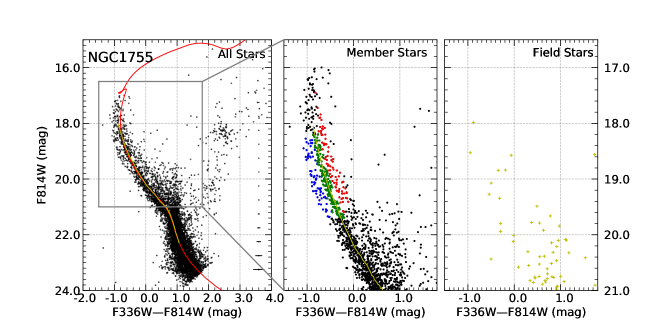
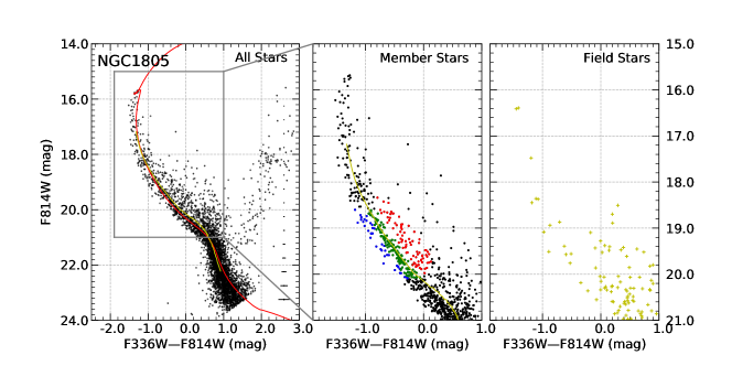
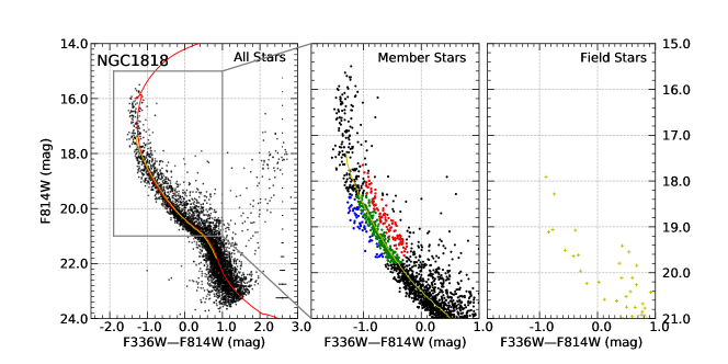
Figure 1: CMDs of NGC 1755, NGC 1805, and NGC 1818. (left) All stars (black points) in the F814W versus (F336W – F814W) CMD. The best-fitting isochrones and ridge lines are shown as red and yellow solid lines, respectively. Error bars on the right of each CMD indicate the uncertainties derived from artificial star tests. (middle) Zoomed-in CMDs of stars located inside the full cluster field and the main bifurcated regions, showing blue-MS stars (blue points), red-MS stars (green points), and high-mass-ratio binaries (red points). (right) Field stars (yellow pluses) selected from the peripheries of the fields of view.

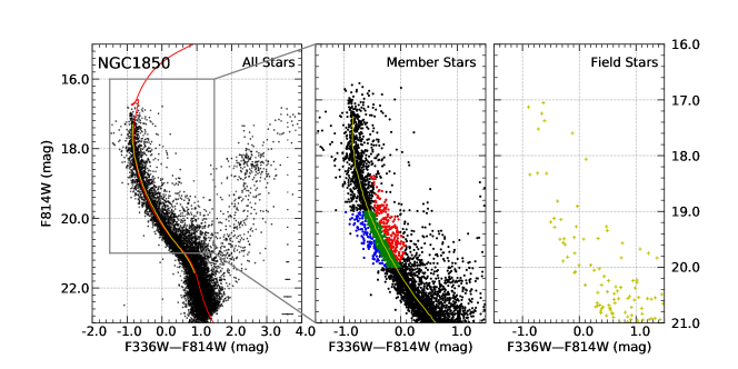
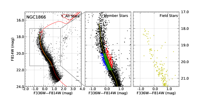
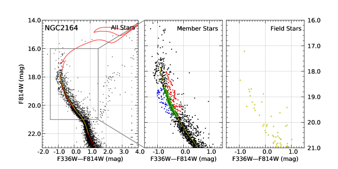
Figure 2: As Figure 1 but for NGC 1850, NGC 1866, and NGC 2164.

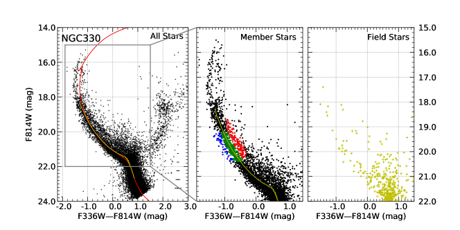
Figure 3: As Figure 1 but for NGC 330.

2.1 Differential reddening

We corrected for differential reddening in the F814W versus (F336W$-$F814W) CMD. Differential reddening may broaden intrinsically narrow stellar sequences in the reddening direction. Milone et al. (2012) described the detailed method we adopted to measure and characterize differential reddening. Briefly, we selected the bulk of the MS stars (whose fiducial line subtends a wide angle with respect to the reddening direction) as our reference population. Then, we rotated the original CMD counterclockwise, adopting the most appropriate angle to align the rotated $x$ axis with the reddening direction, and measured the horizontal distance between the reference stars and their fiducial line. These distances represent the relative reddening suffered by the reference stars compared with the fiducial sequence. For each star in the catalog, the median value of the distances of its 40 (spatially) closest reference stars was assumed as the differential reddening suffered by the target star in this iteration. An improved rotated CMD could be obtained by subtracting the median value from the $x$ value of each star. The newly corrected CMD enabled us to derive a more accurate reference population and a more precise fiducial line for the next iteration. We reran this procedure until the new reference population no longer changed with respect to the previous iteration. The variations in the reddening direction from all iterations were adopted as the final differential reddening value. Finally, we rotated the frame back to obtain the de-reddened CMD.

The relative absorption coefficients at the central wavelengths of the F336W and F814W filters are $\frac{A_{\rm F336W}}{A_{V}}=1.65798$ and $\frac{A_{\rm F814W}}{A_{V}}=0.61018$, respectively, using the Cardelli et al. (1989) and O’Donnell (1994) extinction curves with $R_{V}=3.1$. Among our star clusters, only NGC 1850 exhibits significant differential reddening: $\vartriangle E({\rm F336W}-{\rm F814W})$ ranges from $-0.139\pm 0.008$ mag to $0.120\pm 0.017$ mag. The other five clusters do not exhibit significant variations in $E({\rm F336W}-{\rm F814W})$. As such, the de-reddened data for NGC 1850 and the original data for the other clusters were used for further analysis.

2.2 Isochrone fitting

To derive the ages, metallicities, distance moduli, and reddening values for the seven clusters, we followed the method introduced by Correnti et al. (2016), which assumes that the locus of the bulk of the stars represents the true underlying isochrone of a given cluster. First, we derived the fiducial line in the F814W versus (F336W$-$F814W) CMD based on the 2D probability density function (PDF), calculated based on kernel density estimation (KDE). The point maximizing the PDF marks the starting point of the ridge line. We subsequently traced the ridge line toward both the brighter and fainter sides by moving along the minimum gradient. A bootstrapping approach was applied to measure the true fiducial line and the relevant uncertainties. Specifically, in each round of bootstrapping, we randomly selected a fixed number of stars (half of the total number) as a new data set and used them to derive the ridge line using the method just outlined. After 1000 rounds, an ensemble of ridge-line points was collected for further processing. The total number of points was determined by the length of the step used for the KDE PDF estimation; we adopted 0.01 mag. Then, we distributed all ridge-line points into 0.05 mag bins. The bin center was assumed to be the final fiducial magnitude, and half the bin size was assumed as the error on the magnitude value. The mean value and standard deviation of the color in each bin were assumed as the fiducial color and uncertainty, respectively. The bin size adopted should ensure that each bin contains more than 500 points so as to minimize Poissonian noise.

Second, we compared the fiducial line with a grid of isochrones with varying, reasonable parameters (ages, distance moduli, and reddening values). The grid steps adopted for the latter three parameters were 1 Myr, 0.01 mag, and 0.01 mag, respectively. For the cluster metallicities, we used the typical values, $Z=0.006$ for the LMC and $Z=0.002$ for the Small Magellanic Cloud (SMC). Considering that these parameters are all distributed uniformly, the best-fitting isochrone maximizes the likelihood $\mathcal{L}$,

$$\mathcal{L}\simeq{\rm exp}(-\frac{1}{2}\chi^{2}),$$ (3)

$$\chi^{2}=\sum_{i=1}^{N}\frac{(\vartriangle{\rm col}_{i})^{2}}{\sigma^{2}_{i}},$$ (4)

where $\vartriangle{\rm col}$ is the difference in color between the fiducial line and the isochrone at the same magnitude, and $\sigma$ is the corresponding error. The maximum likelihood corresponds to the best-fitting isochrone. The uncertainty in each best-fitting parameter is assumed as the standard deviation of the Gaussian function that fits the cumulative 1D posterior PDF, which is obtained by marginalizing the 3D posterior PDF over the other two parameters. The best-fitting parameters and their uncertainties are listed in Table 2.

Generally, the distance moduli in Table 2 are slightly smaller than the mean distances to their host galaxies, i.e., $(m-M)_{0}=18.49$ mag for the LMC (de Grijs et al., 2014) and $(m-M)_{0}=18.96$ mag for the SMC (de Grijs & Bono, 2015). Cluster ages derived in this study are slightly older than those derived in the literature. Milone et al. (2018) derived their parameters by fitting blue- and red-MS stars with non- and rapidly rotating isochrones, respectively. The rapidly rotating isochrones yielded ages of 80 Myr, 50 Myr, 40 Myr, 80 Myr, 200 Myr, 100 Myr, and 40 Myr (following the same order as in Table 2). Ahumada et al. (2018, their Table 6) presented a compilation of ages for NGC 1755, NGC 1805, and NGC 1818. The age of NGC 1850 inferred from other studies is generally found in the range 80–100 Myr (e.g., Fischer et al., 1993; Niederhofer et al., 2015; Bastian et al., 2016; Correnti et al., 2017; Yang et al., 2018). Ages reported for NGC 1866 inferred from isochrone modeling range from 140 to 220 Myr (Milone et al., 2017) and those inferred from Cepheids range from 176 to 288 Myr (Costa et al., 2019). Ther ages of NGC 2164 and NGC 330 are $\sim$80–100 Myr (e.g., Mucciarelli et al., 2006; Milone et al., 2018) and $\sim$20–50 Myr (e.g., Keller et al., 2000; Sirianni et al., 2002; McLaughlin & van der Marel, 2005; Li et al., 2017b; Bodensteiner et al., 2020; Carini et al., 2020), respectively.

The degeneracies among age, reddening, and distance modulus may contribute to the large uncertainties associated with those parameters. We note that these parameters should be used with caution for two reasons. First, we adopted non-rotating isochrones to fit the red-MS stars, although they are actually rapidly rotating stars. Second, the accuracy of parameters derived from isochrone fitting is reduced when photometric data includes UV bands. Barker & Paust (2018) compared three stellar evolution models with HST photometric data for two globular clusters in five filters from the UV to the near-infrared. They found that models yield poor fits to CMDs including a UV filter, which may be due to the poorly understood effects of reddening at UV wavelengths. Instead of scrutinizing the specific values of our best-fitting parameters, we focus instead on the clusters’ order, sorted by chronological or dynamical age.

2.3 Selection of bifurcated MS stars

We examined the color variations of the MS stars in our cluster sample and confirmed the presence of bimodal MSs. As an example, Figure 4 (left) shows the zoomed-in CMD of NGC 330, the verticalized CMD (middle), and the color distributions of MS stars in five vertically divided bins (right). The color histograms were fitted using a bi-Gaussian function. The right panel of Figure 4 shows a clear separation between both components in the middle bins, which confirms the split-MS phenomenon. The three subpopulations selected in Figure 5 are also depicted as blue, green, and red points in the left panel of Figure 4. Their loci are consistent with the main bifurcated region.

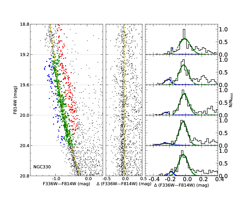
Figure 4: (left) Zoomed-in CMD of stars within the cluster area of NGC 330. The yellow line is the fiducial line of the bulk stellar population. Subpopulations selected from Figure 5 are also presented as blue, green, and red points. (middle) MS stars in the F814W versus $\vartriangle\rm(F336W-F814W)$ diagram. The $x$ axis was obtained by subtracting the fiducial color at the corresponding magnitude for each star. (right) Color histograms in the five vertically divided bins. Blue and green pluses represent the two MS components.

The method used to select split-MS stars is similar to that adopted by Yang et al. (2018). First, the same photometric procedure was applied to artificial stars to derive the photometric errors. Artificial stars were generated with masses following a generic initial mass function (Kroupa, 2001), with magnitudes in F336W and F814W obtained by interpolating the initial masses and magnitudes in the best-fitting isochrone data table and adopting random spatial coordinates across the field of view. We added the artificial stars to the raw images and reran DOLPHOT with the added Fakestars term. To avoid crowding owing to adding artificial stars, we generated 100 stars in each run and collected the input and output catalogs, repeating this approach more than 1000 times for each chip to minimize statistical fluctuations. Comparisons between the input and recovered stars enable us to measure the magnitude uncertainties and also infer the photometric completeness levels.

Table 3: Split-MS regions. (1) Cluster name, (2) Magnitude range, (3) Corresponding mass range, (4) Total number of blue-MS stars, (5) Total number of red-MS stars, (6) Total number of high-mass-ratio binaries, (7) Number of stars within each annular ring.

Cluster	F814W range	Mass range	$N_{\rm bMS}$	$N_{\rm rMS}$	$N_{\rm bin}$	n
	(mag)	($\rm M_{\odot}$)
(1)	(2)	(3)	(4)	(5)	(6)	(7)
NGC 1755	18.2–19.7	2.38–3.68	71	220	79	37
NGC 1805	18.6–20.1	2.10–3.80	40	149	81	27
NGC 1818	18.3–19.8	2.47–4.33	59	264	113	43 (49)
NGC 1850	19.0–20.0	2.35–3.35	113	963	207	128 (131)
NGC 1866	19.5–20.5	1.77–2.46	198	861	209	126 (134)
NGC 2164	18.6–19.8	2.22–3.20	53	264	80	39 (46)
NGC 330	19.2–20.4	2.35–3.81	63	467	150	68

Figure 5 shows the three subpopulations selected from the bimodal-MS region in NGC 330. We will now first introduce the theoretical magnitudes of any unresolved binaries, based on the assumption that no interactions have occurred between both components, and the entire systems would appear as single, point-like sources in distant clusters. The magnitude of a binary system is

$$m_{\rm bin}=m_{\rm 1}-2.5{\rm log}({1+\frac{F_{\rm 2}}{F_{\rm 1}}}),$$ (5)

where $m_{\rm 1}$ is the magnitude of the primary star, and $F_{\rm 1}$ and $F_{\rm 2}$ are the component fluxes. The ratio of the fluxes is in proportion to the mass ratio. At a given primary mass, the brightness of the binary system increases with mass ratio and approaches the brightest point when the two components have identical masses (0.752 mag brighter than the primary star). The main steps involved in drawing the black frames in Figure 5 are as follows. (1) The ridge line (the yellow line in the left panel) obtained in Section 2.2 with 3$\sigma$ errors on the blue side was assumed as the blue boundary for single stars (red-MS stars). (2) Next move the blue boundary pertaining to the single stars arbitrarily to the left to include most stars; the enclosed stars are blue-MS stars. (3) The MS–MS binary sequence with mass ratio $q=0.5$ divides the single stars and unresolved binaries. Stars residing between the binary sequences at $q=0.5$ and $q=1$, including the range encompassed by the 3$\sigma$ color errors, are referred to as high-mass-ratio binaries. (4) The bright and faint cut-offs for MS stars and consistent with the main bifurcated region were inferred from the histograms in Figure 4. The top (bottom) boundary of the high-mass-ratio binary region contains the trajectory of a series of binaries with increasing mass ratio combined with a horizontal line with a width equal to the 3$\sigma$ color error at the corresponding magnitudes. For example, blue-MS stars, red-MS stars, and high-mass-ratio binaries within the cluster field of NGC 330 are shown as blue, green, and red points, respectively, in the left panel of Figure 5. The right panel shows the equivalent distributions of stars in the reference field. A summary of the magnitude bins used to select split-MS stars is presented in Table  3, which also includes the corresponding stellar masses.

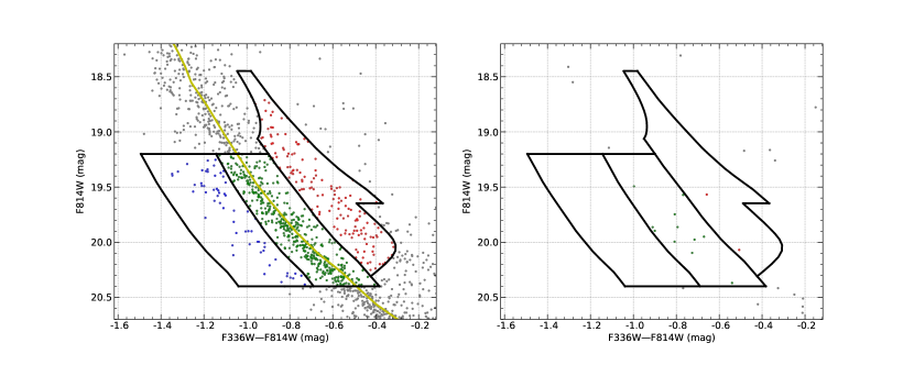
Figure 5: Illustration for NGC 330 of our division of MS stars into three subpopulations for stars located within the cluster and reference fields. The yellow solid line in the left panel is the ridge line calculated based on the 2D KDE PDF. Blue-MS stars, red-MS stars, and high-mass-ratio binaries are shown as blue, green, and red points, respectively. The black frame indicates the boundaries governing the subpopulations. The right panel pertains to stars in the reference field.

2.4 Population Ratios

To study the radial distributions of the selected subpopulations, we divided them into different radial bins. The population ratios of blue-MS stars and high-mass-ratio binaries with respect to the full sample of MS stars are

$$f_{\rm bMS}(r)=\frac{N_{\rm bMS}(r)-A(r)n_{\rm bMS}}{N_{\rm bMS}(r)+N_{\rm rMS}(r)+N_{\rm bin}(r)};$$ (6)

$$f_{\rm bin}(r)=\frac{N_{\rm bin}(r)-A(r)n_{\rm bin}}{N_{\rm bMS}(r)+N_{\rm rMS}(r)+N_{\rm bin}(r)}.$$ (7)

where $N_{\rm bMS}(r)$, $N_{\rm rMS}(r)$, and $N_{\rm bin}(r)$ are, respectively, the numbers of blue-MS stars, red-MS stats, and high-mass-ratio binaries within radius $r$; $n_{\rm bMS}$, $n_{\rm rMS}$, and $n_{\rm bin}$ are the numbers of field stars located in the same CMD area as the three subpopulations. $A(r)$ is the area ratio of the cluster field within $r$ and the reference field. All selected stars were divided equally into annular rings. The total number of the three populations and the numbers of stars in the annular rings are summarized in Table  3. The values in brackets are the numbers of stars in the outermost ring if the mean is not an integer. The calculated population ratios are shown in Figures 6 and 7.

The terms $A(r)n_{\rm bMS}$ and $A(r)n_{\rm bin}$ aim to minimize the effects of field stars. Field-star decontamination was applied under the assumption that the field-star CMD does not depend on the spatial coordinates. As such, the CMD of the field stars behind the cluster region would be similar to that of the reference stars. The area ratio $A(r)$ was calculated using Monte Carlo simulations. Given the limited field of the view of the HST camera, we selected the images’ margins as our reference fields. Rectangular areas far from the cluster center were adopted as reference fields, except for NGC 1818 and NGC 1866. Different reference areas were selected for the latter two clusters, including two field corners for NGC 1818 and the outermost periphery for NGC 1866.

3 Results

Figure 6: Cumulative population ratios of blue-MS stars (blue squares) and high-mass-ratio binaries (red triangles) with respect to the full samples of MS stars as a function of radial distance. Cluster names (NGC 1755, NGC 1818, NGC 1850, and NGC 330) as well as the Pearson correlation coefficients between the two profiles are shown in the panel titles. ‘Error bars’ along the $x$ axis represent the widths of the annular rings; those along the $y$ axis are Poissonian errors. The orange vertical lines indicate the derived half-mass radii.

Figure 7: As Figure 6, but for NGC 1805, NGC 1866, and NGC 2164.

The stellar spatial distribution is a vital ingredient to understand star cluster formation and evolution. Figures 6 and 7 show the cumulative population ratios of blue-MS stars and high-mass-ratio binaries as a function of cluster-centric distance. For each cluster, all bifurcated stars were equally divided into 10 annular rings. These figures show that the two cumulative radial population ratios in NGC 1755, NGC 1818, NGC 1850, and NGC 330 (see Figure 6) are strongly anti-correlated, while no significant relationship between the population ratios was found in NGC 1805, NGC 1866, or NGC 2164 (see Figure 7).

In the first group of clusters, the cumulative population ratio of the high-mass-ratio binaries generally decreases from the inner region to the periphery, while the blue-MS stars’ profile increases. For example, in the case of NGC 1755, the red profile drops from 35.0% to 18.5%, while the blue profile rises from 8.1% to 17.7%, indicating a higher percentage of high-mass-ratio binaries in the core region and the gradually increasing importance of blue-MS stars in the outer regions. Similar profiles were also found for NGC 1818 and NGC 330, but with smaller amplitudes. It is hard to conclude that the two populations in NGC 1850 exhibit monotonous trends; their opposite behavior results in a negative Pearson relation coefficient. Similar trends for split-MS stars selected based on F438W versus (F336W$-$F438W) CMD analysis have been observed for NGC 1850 by Yang et al. (2018).

In the second group of clusters, no significant correlation was found. NGC 1805 contains the fewest split-MS stars (27 stars in each bin), thus contributing large uncertainties to the population ratios. Adopting a larger bin size, e.g., 50 stars in each annular ring, would reduce the fluctuations. The top left panel of Figure 7 shows that the binary profile in NGC 1805 first decreases and then slightly increases at the tail end (large radii), while the blue-MS profile slightly decreases within the first three points, resulting in a low negative correlation. In NGC 1866, the trends in the two profiles result in a medium negative correlation. Following Milone et al. (2017), who also studied the annular population ratios of blue-MS stars and high-mass-ratio binaries, we calculated the annular population ratios of split-MS stars selected from the same magnitude ranges and the same radial bin intervals. The results generally agree with the literature (see Milone et al., 2017, their Figure 9), showing a higher fraction of blue-MS stars to high-mass-ratio binaries beyond the cluster core region. The agreement with Milone et al. (2017) confirms the accuracy of our photometry and data analysis approach. In NGC 2164, even though the fraction of high-mass-ratio binaries decreases as a function of cluster-centric distance, no significant anti-correlation was found between both profiles.

We ran $N$-body simulations to check the spatial distribution of binary systems in an isolated cluster using the high-performance code PeTar (Wang et al., 2020). The initial particle masses, three-dimensional positions, and velocities were generated by the updated star cluster initial model generator code MCLUSTER (Küpper et al., 2011; Wang et al., 2019). We generated a total of 100,000 particles (including 30,000 randomly paired binaries), following a Plummer density profile with the following parameters: degree of mass segregation, $S=0$ (no segregation); fractal dimension, $D=3.0$ (no fractality); virial ratio, $Q=0.5$; half-mass radius, $R_{\rm h}=0.5$ pc; and a Kroupa (2001) initial mass function. The semi-major axis of the binary population was assigned following Kroupa (1995a, b) and Sana et al. (2012) using period distributions for the binaries’ primary components with masses $<5M_{\odot}$ and higher than the mass threshold, respectively. The simulated cluster was evolved to a maximum age of 300 Myr, yielding output snapshots in time intervals of 1 Myr. The snapshot data were first processed with the built-in tools within PeTar to detect binaries and calculate parameters including the Lagrangian and core radii, average masses, and velocity dispersions.

Binary systems can be classified as hard or soft by comparing their binding energy with the surrounding population’s kinetic energy. The boundary between soft and hard binaries is derived as

$$a_{\rm hs}=\frac{GM_{\rm 1}M_{\rm 2}}{3\langle M_{\rm T}\rangle\sigma_{\rm v,3D}^{2}},$$ (8)

where $\langle M_{\rm T}\rangle$ is the average mass of the surrounding stars and $\sigma_{\rm v,3D}$ is the three-dimensional velocity dispersion. Binaries with $a_{\rm hs}$ larger than their semi-major axis are classified as soft binaries; otherwise, they are classified as hard binaries. The different spatial distributions of the two types of binaries can be predicted, since soft binaries become softer and hard binaries get harder after numerous encounters with neighboring stars.

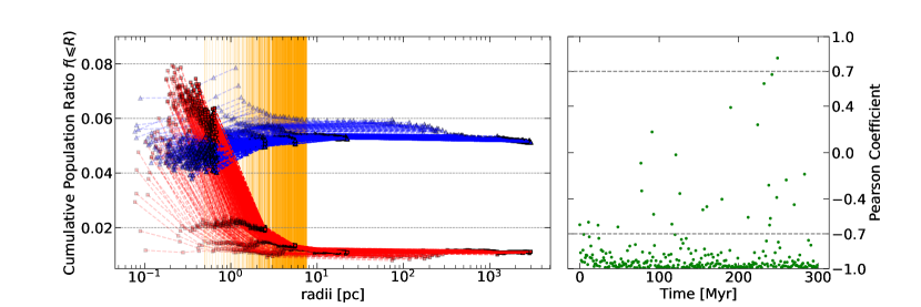
Figure 8: $N$-body simulation results. (left) Secular evolution of the cumulative population ratios of hard and soft binaries. Based on each snapshot, five blue triangles (red squares) indicate the number fractions of soft (hard) binaries within the 10%, 30%, 50%, 70%, and 90% Lagrangian radii. Orange vertical lines indicate the 50% Lagrangian radius, which expands with time. The evolutionary timescale is encoded in the transparency of the lines. (right) Pearson correlation coefficient between the two profiles as a function of evolution timescale.

Our $N$-body simulation suggests that the anti-correlation found in the first four clusters may be associated with their binaries’ dynamical evolution. The left and right panels of Figure 8 show the cumulative number fractions of, respectively, hard binaries (red squares) and soft binaries (blue triangles) in all snapshots and the corresponding Pearson correlation coefficients. For each snapshot, the number ratio of hard/soft binaries with respect to the whole sample was measured at five radial distances (10%, 30%, 50%, 70%, and 90% Lagrangian radii). The radius of the outermost bin and the 50% Lagrangian radius grow with time, indicating cluster expansion at a young age. In general, soft binaries apparently dissolve within the first 20 Myr and the dissolution subsequently slows down due to violent relaxation and two-body relaxation; hard binaries continuously grow due to the hardness of primordial binaries and the newly formed dynamical binaries. A high stellar density reinforces the dissolution or formation of binaries in the core region, which can be inferred from the significant increase in the population ratios in the innermost bin. We calculated the population ratios in each snapshot. The profile of the soft binaries rises as the cluster radius moves outward, while the profile of hard binaries declines. The increasing or decreasing trend is enhanced as a function of time.

The right panel of Figure 8 shows the Pearson correlation coefficients relating the two profiles (green dots), with grey dashed lines showing the criteria for strong correlation, i.e., an absolute value of the coefficient greater than 0.7. Most of the green dots have values $<-0.7$, indicating a strong negative relationship between the spatial distribution profiles of the soft and hard binaries.

We also checked the radial distributions of the binaries divided by other parameters, such as orbital period and mass ratio. The cumulative population ratios of short- and long-period binaries are negatively correlated, while those of low- and high-mass-ratio binaries are positively correlated. This can be expected, since most short-period binaries are hard binaries and binary dissolution has only a minor dependence on their mass ratios.

Our simulation results provide detailed information about the distribution of binaries in an isolated cluster, which can help us constrain the origin of blue-MS stars. In view of a star cluster’s dynamical evolution, primordial binaries go through a rapid dissolution period (continuing for about 20 Myr) during their violent relaxation phase. Subsequently, two-body interaction dominates the dynamics, which reduces the dissolution rate. We analyzed the population ratios of various stellar populations at an age of 150 Myr as a concrete example. The fraction of binaries with mass ratio $q\geq 0.5$ declines from 6.8% to 4.2% when the volume expands from the 10% to the 90% Lagrangian radii. This is consistent with the decreasing radial trend of high-mass-ratio binaries in our observations. Varying the number of initial binaries can adjust the final percentage to agree with the observations. The population ratios of blue-MS stars and simulated soft binaries both increase from the cluster core to the outskirts, but their percentages differ significantly. In the simulation, soft binaries occupy almost 80% of the entire binary population after the violent dissolution phase, a much higher percentage than that of binaries with mass ratios $q\geq 0.5$ (which is around 60%). Constraining the soft binary population by their mass ratios, periods, or other parameters may lower the percentage value and retain an increasing cumulative profile. However, the observational data do not support such approaches. Thus, we speculate that blue-MS stars are, at least in part, soft binaries, and their dissolution leads to the observed dip in the cluster center. The full ingredients of blue-MS stars can only be confirmed once more observational data become available.

4 Discussion

The reason for the different spatial distributions of blue-MS stars and high-mass-ratio binaries into the two groups of clusters is not clear. The split-MS stars generally range from 18.2 mag to 20.5 mag, with slight variations from cluster to cluster. The corresponding mean masses of red-MS stars in the first group of clusters are generally larger than those in the second group, indicating the anti-correlated distributions in the young massive populations. However, NGC 1805 is an exception. Its split-MS stars are as massive as those in NGC 1818, but we did not find a strong relationship between its stellar populations. NGC 1805 and NGC 1818 have similar masses and ages but different dynamical ages. The dynamical ages are the ratios of the clusters’ ages and their half-mass relaxation timescales. The half-mass relaxation timescale is given by (Meylan, 1987)

$$t_{\rm rh}=(8.92\times 10^{5}{\rm yr})\frac{(M/1M_{\odot})^{1/2}}{(\bar{m}/1M_{\odot})}\frac{(r_{\rm h}/1\,{\rm pc})^{3/2}}{\log(0.4M/\bar{m})},$$ (9)

where $M$ is the total cluster mass, $\bar{m}$ is the average mass of its member stars, and $r_{\rm h}$ is the half-mass radius. We derived dynamical ages for all seven clusters and ordered them from dynamically young to old— NGC 1850, NGC 330, NGC 1818, NGC 1866, NGC 1755, NGC 1805, NGC 2164—which is consistent with the order estimated by McLaughlin & van der Marel (2005) (the latter study did not include NGC 1755). Thus, we suggest that the anti-correlation shown in four of our clusters is likely related to both their chronological and dynamical ages.

Note that the Pearson coefficient may vary for the magnitude ranges applied to select bifurcated MS stars. As described in Section  2.3, the magnitude cuts were visually inferred from the color histograms of Figure  4. To check the influence of our visual inspection, we compared the spatial distributions of stars within the same mass range (2.5–3.2 $M_{\odot}$) in all clusters (NGC 1866 was not included since its average mass is much smaller than the other cluster masses). The results showed a medium negative correlation in NGC 1850 and NGC 330. The reduced number of analyzed stars may contribute to this variation. Nevertheless, a shortage of blue-MS stars in the centers of those clusters was also observed, thus supporting our main conclusion that blue-MS stars may be partially associated with soft binaries. Considering the large uncertainties in stellar masses inferred from the best-fitting isochrones and the small numbers of bifurcated stars, we only applied magnitude cuts.

Does the observed spatial distribution originate from the clusters’ initial conditions? We applied Kolmogorov–Smirnov (K–S) tests to quantify the influence of the initial conditions. As dynamic processes are more intensive in the center than in the periphery, the outer regions may still retain traces of the initial distribution. Comparing the bifurcated MS stars’ radial behavior within the half-mass radius and across the full cluster field may reveal signatures of the initial distribution. For high-mass-ratio binaries, K–S tests in the inner region generally yield $p$ values greater than 0.5, indicating that they have similar radial distributions as the red-MS population. The similarity decreases when we enlarge the area to encompass the entire cluster field; the $p$ values in some clusters are low enough to reject the null hypothesis that the two population were drawn from the same distribution (e.g., $p=0.06$ for NGC 2164). For blue-MS stars, the $p$ values pertaining to NGC 1818 and NGC 330 within the half-mass radius are lower than the significance level of 0.05 and become larger when K–S tests are applied to populations within the entire cluster field; the opposite applies to NGC 1850 and NGC 1866, i.e., the $p$ values within the entire cluster field are $<0.05$. K–S tests applied to the blue- and red-MS stars in the other three clusters yield $p$-values larger than 0.1 at different radii. The blue-MS stars’ small numbers may contribute to the uncertainties, since the K–S test’s statistical power increases with sample size. Significant contamination by field stars in the outer regions also affects the K–S test’s accuracy. In summary, we cannot conclude whether the observed radial distributions are the result of dynamical processes or retained from the initial conditions.

The dynamical stage of a star cluster can also be reflected by a population’s cluster-centric concentration. The parameter $A^{+}$ was used to evaluate the concentration of stars. It was introduced by Alessandrini et al. (2016) to measure the central concentration of blue straggler stars. The value of $A^{+}$ represents the area enclosed by the cumulative distributions of the population of interest and the reference population,

$$A^{+}(x)=\int^{x}_{x_{\rm min}}\phi_{\rm BSS}(x^{\prime})-\phi_{\rm REF}(x^{\prime}){\rm d}x^{\prime},$$ (10)

where $x=\log(r/r_{\rm h})$ is the logarithm of the cluster-centric distance normalized to the half-mass radius, $r_{\rm h}$, and $x_{\rm min}$ is the minimum value. We calculated the $A^{+}$ values of the populations in Figures 6 and 7, selecting red-MS stars within the same spatial area as the reference population. In NGC 1755 and NGC 1818, high-mass-ratio binaries have positive $A^{+}$ values, and blue-MS stars have negative $A^{+}$ values in all radial bins. This clear separation indicates that high-mass-ratio binaries are more concentrated than blue-MS stars. The binaries’ higher $A^{+}$ values were also observed in NGC 1850 and NGC 2164, although their values overlapped somewhat with the $A^{+}$ of blue-MS stars. In NGC 1805, NGC 1866, and NGC 330, no significant differences were spotted between the populations’ $A^{+}$ values. All clusters in Figure 6, except NGC 330, exhibit a strong concentration of high-mass-ratio binaries. In two-body encounters, the more massive star loses energy and moves inward, while the less massive star gains energy and moves outward. Cumulative two-body interactions lead to mass segregation, where more massive stars sink to the cluster center, while less massive stars predominantly populate the outer regions of the cluster. The segregation timescale of a star is inversely proportional to its stellar mass, i.e., massive stars need a shorter time to sink to the center. Therefore, it can be expected that $A^{+}$ of the massive population increases with a cluster’s dynamical age, and studies show that $A^{+}$ is a good dynamical indicator for globular clusters. However, the effect of the initial distribution on $A^{+}$ is non-negligible. In addition, the small mass differences between the population of interest and the reference population and the different tidal forces exerted by their host galaxies also affect the accuracy of $A^{+}$ as dynamical indicator in our young cluster sample.

Their spatial distributions offer a new perspective to analyze the origin of the blue-MS stars. In recent years, direct measurements of projected stellar rotation rates in young clusters have revealed bimodal distributions, which is consistent with the observed color bimodality in the split-MS and eMSTO regions (Sun et al., 2019; Kamann et al., 2020). Although stellar rotation is now widely accepted as the dominant mechanism behind those features, single stars alone, even with different rotation rates, cannot fully explain the observations. In the framework of the rotation-spread scenario, the blue- and red-MS stars would have similar spatial distributions since there is no significant mass difference between single slow- and fast-rotators. The K–S tests applied to the two populations and the concentration measurements in this paper are indicative of the different spatial distributions.

D’Antona et al. (2017) showed that varying the rotation rates alone is not sufficient to cover the upper blue-MS. To explain the large number of slowly rotating massive stars, they linked binary interactions to the rotation-spread scenario. D’Antona et al. (2017) suggested that the slow rotators may initially have been rapidly rotating stars that subject to recent braking. Interior material mixing induced by rotation at early times makes them look younger than their non-braked counterparts. The properties of the younger, non-rotating population are in good agreement with those of the upper blue-MS stars. If tidal torques cause the braking, the upper blue-MS stars would actually be binary stars. Sun et al. (2019) also suggested that slow rotators in the open cluster NGC 2287 may have been slowed down by their binary components. Efficient interactions require small separations between the two components, which initially suggest the blue-MS stars are, at least in part, hard binaries. However, the observed spatial distribution suggests a conclusion to the contrary. Our simulation shows that the central concentration of the hard binaries and the radially decreasing profile of the cumulative population ratios is enhanced with time. The radial profile of the soft binaries is more consistent with that of the observed blue-MS stars, leading us to conclude that blue-MS stars are associated with soft binaries. It therefore appears that our observations add more questions about the origin of the blue-MS stars.

We note that velocity dispersion information may be used to disentangle these binary scenarios, since short-period binaries would have higher radial-velocity dispersions. We used the measured heliocentric radial velocities of 14 blue-MS stars and 16 red-MS stars in NGC 1818 (Marino et al., 2018b); their radial-velocity dispersions were 9.50 km s^-1 and 5.76 km s^-1, respectively. However, given the prevailing uncertainties, there are no significant differences between these values.

The external environment—such as tidal forces and binarity—also affects a cluster’s dynamical evolution and may change the stellar radial distribution. Clusters experience different tidal forcing due to their host galaxies, resulting in distinctive spatial behavior. Studies (e.g., Piatti et al., 2019; Piatti & Mackey, 2018; Piatti, 2021) show that differential tidal effects lead to variations in the structural parameters and the internal dynamical evolution of stars in the Milky Way and MC clusters. In this paper, NGC 1850 is located in the LMC’s bar structure. It is subject to stronger tidal forces than the other clusters. Moreover, the MCs host a large number of binary clusters. Bhatia et al. (1991) showed that NGC 1850 is a member of a cluster pair. Bica et al. (1999) also identified NGC 1755 and NGC 1818 as members of binary clusters and NGC 1850 as a member of a triple cluster. The tidal force between a cluster pair or among multiple-cluster systems can accelerate their dynamical evolution, especially if the components have comparable masses. Although simulating the tidal force of each cluster is beyond this paper’s scope, we should nevertheless take the external environment into consideration when we study the spatial distribution of stars in clusters.

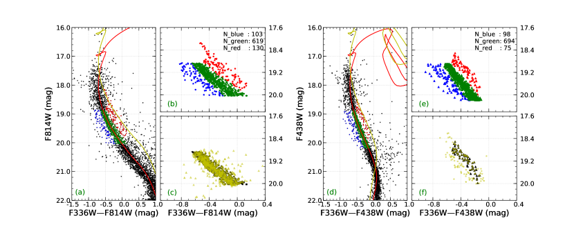
Figure 9: Discrepancies between subpopulations selected from two different NGC 1850 CMDs. The left panels show stars in the F814W versus (F336W$-$F814W) CMD, and the right panels show stars in the F438W versus (F336W$-$F438W) CMD. Black points in panels (a) and (d) show all stars in the cluster region, with stars classified as blue-MS stars, red-MS stars, and high-mass-ratio binaries in the main split region shown as blue, green, and red points, respectively. The red (yellow) solid line indicates the best-fitting isochrone (equal-mass binary sequence). Panels (b) and (e) show a zoomed-in version of the three populations, with individual numbers shown in the top-right corners. Panels (c) and (f) show comparisons of red-MS stars and high-mass-ratio binaries selected from both CMDs. Black symbols indicate stars selected from the same frame and yellow symbols indicate stars selected from different frames.

We note the discrepancies in the NGC 1850 population ratios between stars selected from the F814W versus (F336W$-$F814W) CMD (this paper) and the F438W versus (F336W$-$F438W) CMD (Yang et al., 2018). On the one hand, the two profiles in this paper show more fluctuations, and the decrease or increase is not as strong as that presented in Yang et al. (2018). On the other hand, the number of high-mass-ratio binaries is always larger than that of the blue-MS stars. To fully understand the properties of the stellar populations in different CMDs, we collected raw images observed through the F336W and F438W filters from program GO-14069 (PI: N. Bastian) and images in F275W and F814W from program GO-14174 (PI: P. Goudfrooij) using UVIS/WFC3 on board the HST. The post-pipeline processing, photometric approach, and data selection criteria were identical to the method introduced in Section 2. The final catalog contains stellar magnitudes in four filters.

Differences in the two sets of subpopulations—selected from the F814W versus (F336W$-$F814W) and the F438W versus (F336W$-$F438W) CMDs—are shown in Figure 9. Panels (a) and (d) show the distributions of all stars in the two CMDs and highlight the main split regions; zoomed-in versions are shown in panels (b) and (e). We note the different numbers of stellar populations in the main split region, particularly for high-mass-ratio binaries. The number of binaries (130) selected from panel (b) is nearly twice larger than the number of binaries (75) in panel (e). Panel (f) shows binaries in the UV–infrared CMD (yellow asterisks) that overlap with binaries in the UV–optical CMD (black triangles). It is clear that the yellow asterisks cover a wider area than the black triangles; see also the inconsistency with the red-MS stars in panel (c). Therefore, some red-MS stars may instead be classified as blue-MS stars or high-mass-ratio binaries. The smaller number of high-mass-ratio binaries of Yang et al. (2018) led to the two profiles to cross.

The reason for the increased scatter is not yet clear. One possible explanation is found in interactions between binary stars. The theoretical MS–MS binary sequence was calculated by adding the luminosities of two individual stars, as in Equation 5. However, the effects imposed by companions may not follow this equation, particularly in the case of close binary systems. This inconsistency in stellar positions in different CMDs may indicate that the spectral energy distributions of some stars are not as simple as the theoretical predictions. A filter combination with a longer color baseline is recommended to select stars in CMDs.

5 Summary

We derived high-precision photometry from HST images of seven MC clusters to study the spatial distributions of their blue-MS stars. Stars located in the split-MS region were classified into three populations, including blue-MS stars, red-MS stars, and high-mass-ratio binaries. The cumulative population ratios in 10 radial bins out to the clusters’ outer regions were calculated. The results show that the population ratios of high-mass-ratio binaries to blue-MS stars in four of our clusters (NGC 1755, NGC 1818, NGC 1850, and NGC 330; see Figure 6) are strongly anti-correlated, while no prominent relationship was found for our other three sample clusters (NGC 1805, NGC 1818, and NGC 2164; see Figure 7).

Generally, the number fraction of high-mass-ratio binaries with respect to the total number of MS stars analyzed decreases as a function of the radial distance from the cluster center, while the fraction of blue-MS stars increases. We analyzed the mass range of the bifurcation in each cluster, and the dynamical stage of the cluster based on their dynamical age ${t_{\rm iso}}/{t_{\rm rh}}$ and the dynamical indicator $A^{+}$. The clusters in Figure 6 are young, containing more massive split-MS stars. At the same time, they are also dynamically young. An $N$-body simulation of 100,000 particles, with 30% binary systems and a Plummer density profile, was run. It showed that the dissolution of soft binaries dominates a cluster’s dynamical evolution in the first $10^{8}$ years. Thus, we suggest that the increasing trend of the blue-MS stars’ radial profile may be associated with intensive binary dissolution in the cluster cores.

The observed spatial distributions suggest that blue-MS stars are partly soft binaries, which is at odds with the rotation-spread scenario that interprets them as hard binaries. Our work places new constraints on the origin of blue-MS stars. We note that the classification of the three subpopulations, the radial bin size, and the selected field stars may affect the accuracy of the observed radial profiles. The external environment may affect the spatial distributions of the stellar components. More information is needed to reveal the origin of blue-MS stars.

References

- Ahumada et al. (2018) Ahumada, A. V., Vega-Neme, L. R., Clariá, J. J., & Minniti, J. H. 2018, PASP, 131, 024101, doi: 10.1088/1538-3873/aae660
- Alessandrini et al. (2016) Alessandrini, E., Lanzoni, B., Ferraro, F. R., Miocchi, P., & Vesperini, E. 2016, ApJ, 833, 252, doi: 10.3847/1538-4357/833/2/252
- Astropy Collaboration et al. (2013) Astropy Collaboration, Robitaille, T. P., Tollerud, E. J., et al. 2013, A&A, 558, A33, doi: 10.1051/0004-6361/201322068
- Barker & Paust (2018) Barker, H., & Paust, N. E. Q. 2018, PASP, 130, 034204, doi: 10.1088/1538-3873/aaa597
- Bastian & de Mink (2009) Bastian, N., & de Mink, S. E. 2009, MNRAS, 398, L11, doi: 10.1111/j.1745-3933.2009.00696.x
- Bastian et al. (2020) Bastian, N., Kamann, S., Amard, L., et al. 2020, MNRAS, 495, 1978, doi: 10.1093/mnras/staa1332
- Bastian et al. (2018) Bastian, N., Kamann, S., Cabrera-Ziri, I., et al. 2018, MNRAS, 480, 3739, doi: 10.1093/mnras/sty2100
- Bastian et al. (2016) Bastian, N., Niederhofer, F., Kozhurina-Platais, V., et al. 2016, MNRAS, 460, L20, doi: 10.1093/mnrasl/slw067
- Bastian et al. (2017) Bastian, N., Cabrera-Ziri, I., Niederhofer, F., et al. 2017, MNRAS, 465, 4795, doi: 10.1093/mnras/stw3042
- Bhatia et al. (1991) Bhatia, R. K., Read, M. A., Hatzidimitriou, D., & Tritton, S. 1991, A&AS, 87, 335
- Bica et al. (1999) Bica, E. L. D., Schmitt, H. R., Dutra, C. M., & Oliveira, H. L. 1999, AJ, 117, 238, doi: 10.1086/300687
- Bodensteiner et al. (2020) Bodensteiner, J., Sana, H., Mahy, L., et al. 2020, A&A, 634, A51, doi: 10.1051/0004-6361/201936743
- Bressan et al. (2012) Bressan, A., Marigo, P., Girardi, L., et al. 2012, MNRAS, 427, 127, doi: 10.1111/j.1365-2966.2012.21948.x
- Cardelli et al. (1989) Cardelli, J. A., Clayton, G. C., & Mathis, J. S. 1989, ApJ, 345, 245, doi: 10.1086/167900
- Carini et al. (2020) Carini, R., Biazzo, K., Brocato, E., Pulone, L., & Pasquini, L. 2020, AJ, 159, 152, doi: 10.3847/1538-3881/ab7334
- Correnti et al. (2016) Correnti, M., Gennaro, M., Kalirai, J. S., Brown, T. M., & Calamida, A. 2016, ApJ, 823, 18, doi: 10.3847/0004-637X/823/1/18
- Correnti et al. (2017) Correnti, M., Goudfrooij, P., Bellini, A., Kalirai, J. S., & Puzia, T. H. 2017, MNRAS, 467, 3628, doi: 10.1093/mnras/stx010
- Costa et al. (2019) Costa, G., Girardi, L., Bressan, A., et al. 2019, A&A, 631, A128, doi: 10.1051/0004-6361/201936409
- D’Antona et al. (2015) D’Antona, F., Di Criscienzo, M., Decressin, T., et al. 2015, MNRAS, 453, 2637, doi: 10.1093/mnras/stv1794
- D’Antona et al. (2017) D’Antona, F., Milone, A. P., Tailo, M., et al. 2017, Nat. Astron., 1, 0186, doi: 10.1038/s41550-017-0186
- de Grijs & Bono (2015) de Grijs, R., & Bono, G. 2015, AJ, 149, 179, doi: 10.1088/0004-6256/149/6/179
- de Grijs et al. (2014) de Grijs, R., Wicker, J. E., & Bono, G. 2014, AJ, 147, 122, doi: 10.1088/0004-6256/147/5/122
- Dolphin (2016) Dolphin, A. 2016, DOLPHOT: Stellar photometry. http://ascl.net/1608.013
- Dufton et al. (2013) Dufton, P. L., Langer, N., Dunstall, P. R., et al. 2013, A&A, 550, A109, doi: 10.1051/0004-6361/201220273
- Dupree et al. (2017) Dupree, A. K., Dotter, A., Johnson, C. I., et al. 2017, ApJ, 846, L1, doi: 10.3847/2041-8213/aa85dd
- Elson et al. (1987b) Elson, R. A. W., Fall, S. M., & Freeman, K. C. 1987b, ApJ, 323, 54, doi: 10.1086/165807
- Fischer et al. (1993) Fischer, P., Welch, D. L., & Mateo, M. 1993, AJ, 105, 938, doi: 10.1086/116483
- Georgy et al. (2019) Georgy, C., Charbonnel, C., Amard, L., et al. 2019, A&A, 622, A66, doi: 10.1051/0004-6361/201834505
- Girardi et al. (2013) Girardi, L., Goudfrooij, P., Kalirai, J. S., et al. 2013, MNRAS, 431, 3501, doi: 10.1093/mnras/stt433
- Gonzaga et al. (2012) Gonzaga, S., Hack, W., Frucher, A., & Mack, J. 2012, The DrizzlePac Handbook. (Baltimore, STScI)
- Hunter (2007) Hunter, J. D. 2007, Comput. Sci. Eng., 9, 90, doi: 10.1109/MCSE.2007.55
- Kamann et al. (2018) Kamann, S., Bastian, N., Husser, T. O., et al. 2018, MNRAS, 480, 1689, doi: 10.1093/mnras/sty1958
- Kamann et al. (2020) Kamann, S., Bastian, N., Gossage, S., et al. 2020, MNRAS, 492, 2177, doi: 10.1093/mnras/stz3583
- Keller et al. (2000) Keller, S. C., Bessell, M. S., & Da Costa, G. S. 2000, AJ, 119, 1748, doi: 10.1086/301282
- Kroupa (1995a) Kroupa, P. 1995a, MNRAS, 277, 1491, doi: 10.1093/mnras/277.4.1491
- Kroupa (1995b) —. 1995b, MNRAS, 277, 1507, doi: 10.1093/mnras/277.4.1507
- Kroupa (2001) —. 2001, MNRAS, 322, 231, doi: 10.1046/j.1365-8711.2001.04022.x
- Küpper et al. (2011) Küpper, A. H. W., Maschberger, T., Kroupa, P., & Baumgardt, H. 2011, MNRAS, 417, 2300, doi: 10.1111/j.1365-2966.2011.19412.x
- Li et al. (2016) Li, C., de Grijs, R., Bastian, N., et al. 2016, MNRAS, 461, 3212, doi: 10.1093/mnras/stw1491
- Li et al. (2017a) Li, C., de Grijs, R., Deng, L., & Milone, A. P. 2017a, ApJ, 834, 156, doi: 10.3847/1538-4357/834/2/156
- Li et al. (2017b) —. 2017b, ApJ, 844, 119, doi: 10.3847/1538-4357/aa7b36
- Mackey & Broby Nielsen (2007) Mackey, A. D., & Broby Nielsen, P. 2007, MNRAS, 379, 151, doi: 10.1111/j.1365-2966.2007.11915.x
- Marino et al. (2018a) Marino, A. F., Milone, A. P., Casagrande, L., et al. 2018a, ApJ, 863, L33, doi: 10.3847/2041-8213/aad868
- Marino et al. (2018b) Marino, A. F., Przybilla, N., Milone, A. P., et al. 2018b, AJ, 156, 116, doi: 10.3847/1538-3881/aad3cd
- McLaughlin & van der Marel (2005) McLaughlin, D. E., & van der Marel, R. P. 2005, ApJS, 161, 304, doi: 10.1086/497429
- Meylan (1987) Meylan, G. 1987, A&A, 184, 144
- Milone et al. (2013) Milone, A. P., Bedin, L. R., Cassisi, S., et al. 2013, A&A, 555, A143, doi: 10.1051/0004-6361/201220567
- Milone et al. (2009) Milone, A. P., Bedin, L. R., Piotto, G., & Anderson, J. 2009, A&A, 497, 755, doi: 10.1051/0004-6361/200810870
- Milone et al. (2016) Milone, A. P., Marino, A. F., D’Antona, F., et al. 2016, MNRAS, 458, 4368, doi: 10.1093/mnras/stw608
- Milone et al. (2012) Milone, A. P., Piotto, G., Bedin, L. R., et al. 2012, A&A, 540, A16, doi: 10.1051/0004-6361/201016384
- Milone et al. (2015) Milone, A. P., Bedin, L. R., Piotto, G., et al. 2015, MNRAS, 450, 3750, doi: 10.1093/mnras/stv829
- Milone et al. (2017) Milone, A. P., Marino, A. F., D’Antona, F., et al. 2017, MNRAS, 465, 4363, doi: 10.1093/mnras/stw2965
- Milone et al. (2018) Milone, A. P., Marino, A. F., Di Criscienzo, M., et al. 2018, MNRAS, 477, 2640, doi: 10.1093/mnras/sty661
- Mucciarelli et al. (2006) Mucciarelli, A., Origlia, L., Ferraro, F. R., Maraston, C., & Testa, V. 2006, ApJ, 646, 939, doi: 10.1086/504969
- Niederhofer et al. (2015) Niederhofer, F., Hilker, M., Bastian, N., & Silva-Villa, E. 2015, A&A, 575, A62, doi: 10.1051/0004-6361/201424455
- O’Donnell (1994) O’Donnell, J. E. 1994, ApJ, 422, 158, doi: 10.1086/173713
- Piatti (2021) Piatti, A. E. 2021, arXiv e-prints, arXiv:2101.03157. https://arxiv.org/abs/2101.03157
- Piatti & Mackey (2018) Piatti, A. E., & Mackey, A. D. 2018, MNRAS, 478, 2164, doi: 10.1093/mnras/sty1048
- Piatti et al. (2019) Piatti, A. E., Webb, J. J., & Carlberg, R. G. 2019, MNRAS, 489, 4367, doi: 10.1093/mnras/stz2499
- Sana et al. (2012) Sana, H., de Mink, S. E., de Koter, A., et al. 2012, Science, 337, 444, doi: 10.1126/science.1223344
- Sirianni et al. (2002) Sirianni, M., Nota, A., De Marchi, G., Leitherer, C., & Clampin, M. 2002, ApJ, 579, 275, doi: 10.1086/342723
- STScI Development Team (2013) STScI Development Team. 2013, pysynphot: Synthetic photometry software package. http://ascl.net/1303.023
- Sun et al. (2019) Sun, W., de Grijs, R., Deng, L., & Albrow, M. D. 2019, ApJ, 876, 113, doi: 10.3847/1538-4357/ab16e4
- Wang et al. (2020) Wang, L., Iwasawa, M., Nitadori, K., & Makino, J. 2020, MNRAS, 497, 536, doi: 10.1093/mnras/staa1915
- Wang et al. (2019) Wang, L., Kroupa, P., & Jerabkova, T. 2019, MNRAS, 484, 1843, doi: 10.1093/mnras/sty2232
- Yang et al. (2018) Yang, Y., Li, C., Deng, L., de Grijs, R., & Milone, A. P. 2018, ApJ, 859, 98, doi: 10.3847/1538-4357/aabe26