Parsimonious Inference

Abstract

Bayesian inference provides a uniquely rigorous approach to obtain principled justification for uncertainty in predictions, yet it is difficult to articulate suitably general prior belief in the machine learning context, where computational architectures are pure abstractions subject to frequent modifications by practitioners attempting to improve results. Parsimonious inference is an information-theoretic formulation of inference over arbitrary architectures that formalizes Occam’s Razor; we prefer simple and sufficient explanations. Our universal hyperprior assigns plausibility to prior descriptions, encoded as sequences of symbols, by expanding on the core relationships between program length, Kolmogorov complexity, and Solomonoff’s algorithmic probability. We then cast learning as information minimization over our composite change in belief when an architecture is specified, training data are observed, and model parameters are inferred. By distinguishing model complexity from prediction information, our framework also quantifies the phenomenon of memorization.
Although our theory is general, it is most critical when datasets are limited, e.g. small or skewed. We develop novel algorithms for polynomial regression and random forests that are suitable for such data, as demonstrated by our experiments. Our approaches combine efficient encodings with prudent sampling strategies to construct predictive ensembles without cross-validation, thus addressing a fundamental challenge in how to efficiently obtain predictions from data.

Keywords: Bayesian inference, information, prior belief, Kolmogorov complexity, Solomonoff probability

1 Introduction

We began this investigation desiring to understand the relationship between prior belief and the resulting uncertainty in predictions obtained from inference in the hope that new insights would provide a sound basis to improve prediction credibility in machine learning. The mathematical and epistemological foundations of rational belief, from which the laws of probability and Bayesian inference are derived as an extended logic from binary propositional logic (Cox, 1946), lead us to assert the central role of Bayesian inference in obtaining rigorous justification for uncertainty in predictions. Although this foundation of reason holds generally, it is critical when we need to learn robust predictions from limited datasets. Yet, applying Bayesian inference within the machine learning context requires addressing a fundamental challenge: inference requires prior belief. When the amount of evidence contained within a dataset regarding a phenomenon of interest is extremely limited, specifying prior belief is not merely an inconvenience; it is the dominant source of uncertainty in predictions. Examples of such data limitations include having few observations, noisy measurements, skewed or highly imbalanced labels of interest, or even a degree of mislabeling in the data.

When predictive models integrate well-understood physical principles, they are often accompanied by physically plausible parameter ranges that provide a strong basis for prior belief. Likewise, canonical priors are acceptable for simple approximations with relatively few unconstrained parameters in comparison to the size of the dataset intended for inference. Kass and Wasserman (1996) give a thorough survey of related work. In contrast, the machine learning paradigm seeks to instrument arbitrary algorithms with high parameter dimensionality. A typical architecture may have tens of thousands, or perhaps millions, of free parameters. In this setting, the sensitivity of predictions to an arbitrary choice of prior belief may be unacceptable for applications of consequence (Owhadi et al., 2015).

1.1 Our Contributions

Expanding on the work of Solomonoff (1964a, b, 2009), Kolmogorov (1965), Rissanen (1983, 1984), and Hutter (2007), we develop a theoretical framework that assigns plausibility to arbitrary inference architectures. Just as Solomonoff derives algorithmic probability from program length, the minimum number of bits needed to encode a program for a specified Universal Turing Machine (UTM), we show how a modest generalization yields a universal hyperprior over symbolic encodings of ordinary priors. We may regard an ordinary prior, that which is typically used in Bayesian inference, as a restricted state of belief from a general universe of potential explanatory models. Within our framework, every choice of computational architecture, and associated prior over model parameters, is just a restriction of prior belief. Our hyperprior provides a means to measure and control the complexity of such choices.

We show how our theory of information (Duersch and Catanach, 2020), LABEL:thm:info, allows us to derive a training objective from the information that is created when we select a prior representation, observe the training data, and either infer the posterior distribution or construct a variational approximation of it. Zhang et al. (2018) provide a thorough survey of recent work on variational inference. Our main result, LABEL:thm:parsimony_optimization, clarifies how we may understand learning as an information optimization problem. Our parsimony objective separates into three components:

• Encoding information contained within a symbolic description of prior belief;

• Model information gained through inference using evidence;

• Predictive information gained regarding the observed labels from plausible models.

In our derivation, the first two terms appear with negative signs and the third with a positive sign, revealing how our theory suppresses complexity as an intrinsic tradeoff against increased agreement with observed labels. The first component guards against excessive complexity in our description of prior belief and the second guards against priors that are poorly suited to our data. In contrast, the third component promotes agreement between resulting predictions and the data. The main distinction between the second and third components is that model information is measured in the space of explanations, whereas predictive information measures the result of applying plausible models to our data.

We review work on universal priors over integers, corresponding binary representations, and show how a simple integer encoding approximates the scaling invariance of Jeffreys prior. We then demonstrate this theory with two learning prototypes.

Our first algorithm casts polynomial regression within this framework, predicting a distribution over continuous outcomes from a continuous input. By setting the maximum polynomial degree to be much higher than the data merits, standard machine learning training strategies are susceptible to memorization, as we demonstrate by applying gradient based training with leave-one-out cross-validation. In contrast, our prototype discovers much simpler models from the same high-degree basis. Moreover, when we aggregate predictions over an ensemble of polynomial representations, our prototype demonstrates the natural increase in uncertainty we intuitively associate with extrapolation.

Our second algorithm samples ensembles of decision trees that are constructed using the parsimonious inference objective. These models aim to predict discrete labels through a sequence of partitions on continuous feature coordinates. Our random forest prototype demonstrates the ability to learn credible prediction uncertainty from extremely small and heavily skewed datasets, which we contrast with a standard decision tree model and bootstrap aggregation. Both of these algorithms achieve superior prediction uncertainty through Bayesian inference from prior belief that is derived to both quantify and naturally suppress complexity over arbitrary explanations.

Although our basic hyperprior is subject to a choice of interpreter—which need not be Turing-complete, but must transform valid codes into coherent probability distributions over predictive models—we go on to show that to be consistent with this theory, there exists a unique hyperprior over an ensemble of Turing-complete interpreters, LABEL:thm:utm_ensemble.

1.2 Organization

Section 2 begins with a discussion and illustration of the severe inadequacies of traditional machine learning training approaches that depend on cross-validation. We then briefly review the critical connections between scientific principles, rational belief, and Bayesian inference, which provide a sound theory to obtain rigorously justified uncertainty in predictions. When placed in the machine learning context, however, we explore how principled justification for prior belief over abstract models, as well as our unavoidable disregard for an infinite number of alternative models, remains a critical challenge. Further, we summarize how our theory of information is derived to satisfy key properties that allow us to relate the various forms of complexity that follow in the parsimonious inference objective.

LABEL:sec:complexity continues with our main contributions, including a discussion of generalized description length, a coherent complexity hyperprior, and the principles of minimum information and maximum entropy. These notions culminate in the parsimonious inference objective, providing a suitable framework to understand and control model complexity over arbitrary learning architectures. We also show how this objective allows us to quantify memorization. Our theory allows us to apply these concepts within a wide variety of approaches to solve learning problems, including variational inference techniques.

LABEL:sec:implementation examines implementation details within our prototype algorithms, including efficient encodings and training strategies for polynomial regression and decision trees.

LABEL:sec:discussion concludes with a discussion of how we may consistently compare multiple interpreters, a pathway to frame and address computability à priori, our theory’s relationship to other work, and a summary of our findings.

2 Background

In order to clarify how we may improve trust in machine learning predictions, we must begin with the origin of trust in science. The epistemological foundation of the scientific method shares a fundamental connection with Bayesian inference and determines how we may optimally account for evidence to learn plausible explanations. Bayesian theory alone, however, does not provide a complete learning framework when we employ high-parameter families, such as most machine learning architectures. Thus, we also review Solomonoff’s and Kolmogorov’s notions of complexity as a means to promote simplicity in learned models. To motivate the need for this discussion, we begin by illustrating the severe deficiencies of standard machine learning training practices when they are applied to small datasets.

2.1 Memorization

The term memorization is often conflated with overtraining, but we distinguish these terms as follows. Overtraining is characterized by degradation in prediction quality on unseen data that occurs after an initial stage of improvements. In contrast, memorization refers more generally to any predictive algorithm that exhibits unjustifiable confidence, or low prediction uncertainty, in the training dataset labels that were used to adjust model parameters. LABEL:sec:info_min provides rigorous analysis to justify this view. Conflating these terms leads to an incorrect picture of the problem; to avoid memorization, we must merely halt training at the correct moment.

Machine learning algorithms are typically trained using some variation of stochastic gradient descent (Robbins and Monro, 1951). When applied to overparameterized models, traditional optimization strategies are subject to overtraining. Cross-validation (Allen, 1974) attempts to prevent overtraining by monitoring predictions on a holdout dataset, but we show how this method still fails to prevent memorization on small datasets. The same strategy is also used to tune hyperparameters, such as such as regularization weights and learning-rate schedules.

The obvious difficulty presented by cross-validation is the inherent tradeoff between using as much data as possible to train parameters, but also having a reliable estimator for prediction quality. For limited data, standard practices apply some form of k-fold cross-validation (Hastie et al., 2009). One forms k distinct partitions of the dataset, trains k models respectively, and aggregates predictions by averaging. Leave-one-out cross-validation uses the same number of partitions as datapoints. Each partition reserves only one observation to estimate the best model over each training trajectory.

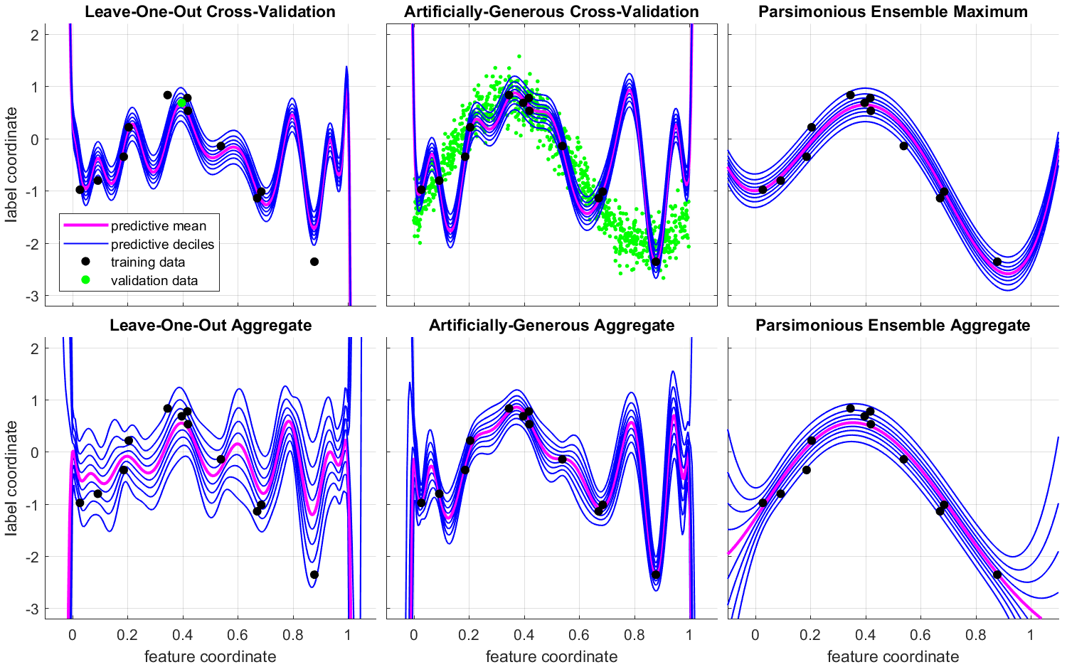
Figure 1: Illustration of standard training shortcomings. Top-left: optimum obtained from holding out the green point. Bottom-left: mean predictions over all single-holdout optima. Top-middle: idealized training on all original data and 1000 extra validation points from ground truth. Bottom-middle: mean predictions over 12 random starts, $\mathcal{N}(\theta_{i}\mid\mu=0,\sigma=0.2)$. Removing the tradeoff between holdout and training data does not prevent complexities in predictions. Top-right: optimal model discovered using our theoretical framework and prototype algorithm. Bottom-right: our aggregate accounts for many plausible models, improving robustness and demonstrating natural extrapolation uncertainty.

Figure 1 demonstrates these techniques using polynomial regression, fitting 20th degree polynomials with only 12 points. Retaining more polynomial coefficients than training points allows us to observe how standard training fails when data are limited. The top-left shows an example of a single model trained by holding out one point for validation, shown in green. The bottom-left shows average predictions over 12 such models. Yet, suppose we could train with all 12 points while remaining highly confident that we will halt training at the correct moment. This ideal is demonstrated as a thought experiment in the middle column of Figure 1 by sampling 1000 extra data from the generative process, the ground truth mechanism that creates observations. We see that eliminating the tradeoff between training and validation would not prevent artifacts from developing that confidently hew to scant observations, memorization.

Typically, one would also use cross-validation to tune the optimal polynomial degree, which would certainly constrain complexity somewhat. The purpose of this experiment, however, is to show that naïve training may never even explore low-complexity models, especially in high dimensions. For most high-parameter families, such as neural networks, there is no feasible hierarchy of bases that would be analogous to limiting the polynomial degree. For example, if we wished to constrain model parameters to a fixed sparsity pattern, the number of patterns to test would grow exponentially in the number of nonzero elements.

This experiment demonstrates how neither of the competing cross-validation objectives address the core problem with learning from limited data. Memorization is often framed in terms of a bias-variance tradeoff; predictions should avoid fluctuating rapidly, but also remain flexible enough to extract predictive patterns. In our theoretical framework, however, memorization is more comprehensively and rigorously understood as unparsimonious model complexity, i.e. increases in model information that are not justified by only small improvements to training predictions.

Regularization strategies attempt to address this heuristically by penalizing excessive freedom in learning parameters, for example attaching an $\ell_{1}$ or $\ell_{2}$ norm to the training objective. While many of these approaches can be equivalently cast as choices of prior belief, they lack a unifying principle that would illuminate and resolve choices of regularization shape and weight. One must, again, resort to hyperparameter tuning via cross-validation, thus failing to address the core challenge: to efficiently learn from limited data.

2.2 Scientific Reasoning and Bayesian Inference

In order to reiterate the concrete relationship between Bayesian inference and scientific reasoning, we review the epistemological foundations of reason at the center of the scientific method. These foundations bear decisive consequences regarding the valid forms of analysis we may pursue in order to obtain rational predictions. At its core, the scientific method relies on coherent mathematical models of observable phenomena that have been informed over centuries of physical measurements. Within the field of epistemology, this is the naturalist view of rational belief (Brandt, 1985). It holds that validity is ultimately derived from consistency, which can be understood in three key components:

1. Rational beliefs must be logical, avoiding internal contradictions;

2. Rational beliefs must be empirical, accounting for all available evidence;

3. Rational beliefs must be predictive, continually reassessing validity by how well predictions agree with new observations.

The third point is really nothing more than a restatement of the second point, placing emphasis on the evolving nature of rational beliefs as new data become available. The critical significance of the first point is that it provides a path to elevate the second and third points to a rigorous extended logic: Bayesian inference.

Building on the rich body of work by many scholars—including Ramsey (2016, original 1926), De Finetti (1937), and Jeffreys (1998, original 1939)—Cox (1946) shows that for a mathematical framework analyzing degrees of truth, belief as an extended logic, to be consistent with binary propositional logic, that formalism must satisfy the laws of probability:

1. Probability is nonnegative.

2. Only impossibility has probability zero.

3. Only certainty has maximum probability, normalized to one.

4. To revise the degree of credibility we assign to a model upon reviewing empirical evidence, we must apply Bayes’ theorem.

Consequently, the Bayesian paradigm provides a uniquely rigorous approach to quantify uncertainty in predictions derived through inductive reasoning. Therefore, the only logically correct path to quantify and suppress memorization in learning must be cast within the Bayesian perspective.

Analysis proceeds with a probability distribution called the prior $\mathbf{p}(\boldsymbol{\theta})$ that quantifies our lack of information, or initial uncertainty, in plausible explanatory models. Here, $\boldsymbol{\theta}$ is any specific parameter state within a model class, or computational architecture. When we need to emphasize the prior’s dependence on a model class, as well as the shape of the parameter distribution within that class, we will write the prior as $\mathbf{p}(\boldsymbol{\theta}\mid\boldsymbol{\psi})$, where a description $\boldsymbol{\psi}$, or hyperparameter sequence, provides such details. We will examine how $\boldsymbol{\psi}$ plays a key role regarding model complexity in detail in LABEL:sec:complexity. The empirical data are expressed as a set of ordered pairs $\mathcal{\mathcal{D}}=\{(\boldsymbol{x}_{i},\boldsymbol{y}_{i})\mid i\in[n]\}$ that have been sampled from the generative process $\mathbf{g}(\boldsymbol{x},\boldsymbol{y})$. Features $\boldsymbol{x}_{i}$ are used to predict labels $\boldsymbol{y}_{i}$ from the architecture paired with $\boldsymbol{\theta}$. We write the predicted distribution over all potential labels as $\mathbf{p}(\boldsymbol{y}_{i}\mid\boldsymbol{x}_{i},\boldsymbol{\theta})$.

If the ordered pairs in $\mathcal{\mathcal{D}}$ represent independent samples from the underlying process, the likelihood is evaluated as $\mathbf{p}(\mathcal{\mathcal{D}}\mid\boldsymbol{\theta})=\prod_{i\in[n]}\mathbf{p}(\boldsymbol{y}_{i}\mid\boldsymbol{x}_{i},\boldsymbol{\theta})$, which expresses the probability of observing $\mathcal{\mathcal{D}}$ if a hypothetical explanation $\boldsymbol{\theta}$ held. Then, we update our beliefs according to Bayes’ theorem. In our picture, we hold that having $\boldsymbol{\theta}$ alone is sufficient to evaluate predictions. When we explicate the role of prior descriptions $\boldsymbol{\psi}$, that means inference can be written as

$$\mathbf{p}(\boldsymbol{\theta}\mid\mathcal{\mathcal{D}},\boldsymbol{\psi})=\frac{\mathbf{p}(\mathcal{\mathcal{D}}\mid\boldsymbol{\theta})\mathbf{p}(\boldsymbol{\theta}\mid\boldsymbol{\psi})}{\mathbf{p}(\mathcal{\mathcal{D}}\mid\boldsymbol{\psi})}\quad\text{where}\quad\mathbf{p}(\mathcal{\mathcal{D}}\mid\boldsymbol{\psi})=\!\int\!d\boldsymbol{\theta}\,\mathbf{p}(\mathcal{\mathcal{D}}\mid\boldsymbol{\theta})\mathbf{p}(\boldsymbol{\theta}\mid\boldsymbol{\psi}$$

is the model-class evidence. If we have a hyperprior $\mathbf{p}(\boldsymbol{\psi})$ over potential descriptions, we can also infer the hyperposterior

$$\mathbf{p}(\boldsymbol{\psi}\mid\mathcal{\mathcal{D}})=\frac{\mathbf{p}(\mathcal{\mathcal{D}}\mid\boldsymbol{\psi})\mathbf{p}(\boldsymbol{\psi})}{\mathbf{p}(\mathcal{\mathcal{D}})}\quad\text{where}\quad\mathbf{p}(\mathcal{\mathcal{D}})=\!\int\!d\boldsymbol{\psi}\,\mathbf{p}(\mathcal{\mathcal{D}}\mid\boldsymbol{\psi})\mathbf{p}(\boldsymbol{\psi})$$

The central point of inference is that it does not attempt to identify a single explanation matching the data, as with stochastic gradient optimization and cross-validation. Rather, inference naturally adheres to the Epicurean principle—we should retain multiple explanations according to their respective degrees of plausibility—within a coherent mathematical framework. As a distribution, the posterior is meaningful in a way that a single model is not; it allows us to update our beliefs consistently as new evidence emerges. We obtain rational predictions by evaluating the posterior predictive integral, or even the hyperposterior predictive integral, respectively constructed as

This result shifts remaining subjectivity to the set of interpreters we are willing to consider for comparison. In practice, the shortest simulator in each set, say $\boldsymbol{\check{\psi}}_{ij}\in\boldsymbol{\Psi}_{ij}$, will dominate the corresponding matrix element. Thus, a more practical approximation of the hyperprior transition matrix is

$$\mathbf{p}(\boldsymbol{\varphi}_{i}\mid\boldsymbol{\varphi}_{j})\approx\left(\sum_{k}2^{-{\mathcal{\ell}}(\boldsymbol{\check{\psi}}_{kj})}\right)^{-1}2^{-{\mathcal{\ell}}(\boldsymbol{\check{\psi}}_{ij})}$$

Note $2^{-{\mathcal{\ell}}(\boldsymbol{\check{\psi}}_{ii})}=1$ for all $i\in[n]$, since the shortest self-simulator is trivial in each language, $\boldsymbol{\check{\psi}}_{ii}=\emptyset$. We find this result intuitive because it suppresses interpreters that require excessive complexity to simulate. In the absence of such a computation, we may only conclude that we should prefer interpreters that appear to be simple.

5.2 Integrating Additional Beliefs

Although this work is motivated by the difficulty of expressing prior belief over abstract models, when we have access to additional information that could constrain prior beliefs, that information may be impactful. Therefore, we should be able to integrate other prior beliefs within the general complexity framework. Let our complexity-based prior belief be denoted as $\mathbf{p}(\boldsymbol{a}\mid\mathcal{C})=2^{-{\mathcal{\ell}}(\boldsymbol{\psi}(\boldsymbol{a}))}$. If we also have other prior beliefs, $\mathbf{p}(\boldsymbol{a}\mid\mathcal{B})$, we can form the composite prior $\mathbf{p}(\boldsymbol{a}\mid\mathcal{B},\mathcal{C})$. For example, $\mathcal{B}$ may express physical laws or previously observed data. One approach would be to use an interpreter that implicitly embeds $\mathcal{B}$ within viable encodings so that $\mathbf{p}(\boldsymbol{a}\mid\mathcal{B},\mathcal{C})=2^{-{\mathcal{\ell}}(\boldsymbol{\psi}_{\mathcal{B}}(\boldsymbol{a}))}$. Alternatively, if we assume that belief derived from $\mathcal{B}$ is conditionally independent of our complexity-based belief $\mathcal{C}$, then we have

Proof of LABEL:cor:probability_from_length. If the encoding is consistent with object probability, and the encoding also maximizes entropy, then

$$\mathbf{p}(\boldsymbol{a})=\prod_{i=1}^{n}\mathbf{p}(\boldsymbol{s}_{i}\mid(\boldsymbol{s})_{1}^{i-1})=\prod_{i=1}^{n}\frac{1}{|\boldsymbol{\Sigma}_{i}|}=2^{-{\mathcal{\ell}}(\boldsymbol{a})}$$

Proof of LABEL:cor:probability_from_length, recursive consistency alternative. We also obtain the same prior by combining a counting argument with consistent prior belief in length descriptions. In order to distinguish a complete short sequence from merely a subsequence of a longer description, we need some indication of the complete sequence length. The following argument holds for descriptions $\boldsymbol{\psi}$ that are capable of being partitioned into a component $\boldsymbol{\psi}_{\boldsymbol{l}}$ that determines the sequence length and the unconstrained complement $\boldsymbol{\psi}_{\boldsymbol{c}}$ so that $\boldsymbol{\psi}=(\boldsymbol{\psi}_{\boldsymbol{l}},\boldsymbol{\psi}_{\boldsymbol{c}})$ and ${\mathcal{\ell}}(\boldsymbol{\psi})={\mathcal{\ell}}(\boldsymbol{\psi}_{\boldsymbol{l}})+{\mathcal{\ell}}(\boldsymbol{\psi}_{\boldsymbol{c}})$. Once $\boldsymbol{\psi}_{\boldsymbol{l}}$ is known, we can easily identify $\boldsymbol{\psi}_{\boldsymbol{c}}$, regardless of its content. Yet, the same problem arises with knowing when we have a complete length description $\boldsymbol{\psi}_{\boldsymbol{l}}$, which can be resolved with recursive partitions $\boldsymbol{\psi}_{\boldsymbol{l}}=(\boldsymbol{\psi}_{\boldsymbol{l}\boldsymbol{l}},\boldsymbol{\psi}_{\boldsymbol{l}\boldsymbol{c}})$ and so on. For the description to be finite, this recursion must end implicitly with only one possible outcome $\boldsymbol{\psi}_{\boldsymbol{l}\ldots\boldsymbol{l}\boldsymbol{l}}=\emptyset$.

We define ${\mathcal{\ell}}(\boldsymbol{\psi}_{\boldsymbol{c}})$ so that the complement allows for $2^{{\mathcal{\ell}}(\boldsymbol{\psi}_{\boldsymbol{c}})}$ outcomes. Binary sequences provide useful intuition for this construction. If we believe all descriptions of a given length have the same prior probability, then

$$1=\!\int\!d\boldsymbol{\psi}_{\boldsymbol{c}}\,\mathbf{p}(\boldsymbol{\psi}_{\boldsymbol{c}}\mid{\mathcal{\ell}}(\boldsymbol{\psi}))=2^{{\mathcal{\ell}}(\boldsymbol{\psi}_{\boldsymbol{c}})}\mathbf{p}(\boldsymbol{\psi}_{\boldsymbol{c}}\mid{\mathcal{\ell}}(\boldsymbol{\psi}))\quad\text{so that}\quad\mathbf{p}(\boldsymbol{\psi}_{\boldsymbol{c}}\mid{\mathcal{\ell}}(\boldsymbol{\psi}))=2^{{\mathcal{\ell}}(\boldsymbol{\psi})-{\mathcal{\ell}}(\boldsymbol{\psi}_{\boldsymbol{l}})}$$

Thus, $\mathbf{p}(\boldsymbol{\psi})=2^{{\mathcal{\ell}}(\boldsymbol{\psi})-{\mathcal{\ell}}(\boldsymbol{\psi}_{\boldsymbol{l}})}\mathbf{p}(\boldsymbol{\psi}_{\boldsymbol{l}})$. But if the length description satisfies a consistent prior to determine our belief in the length of the sequence, we must also have $\mathbf{p}(\boldsymbol{\psi}_{\boldsymbol{l}})=2^{{\mathcal{\ell}}(\boldsymbol{\psi}_{\boldsymbol{l}})-{\mathcal{\ell}}(\boldsymbol{\psi}_{\boldsymbol{l}\boldsymbol{l}})}\mathbf{p}(\boldsymbol{\psi}_{\boldsymbol{l}\boldsymbol{l}})$. This gives

Proof of LABEL:cor:solomonoff. Let $\mathbf{q^{*}}\!(\boldsymbol{a})$ be the optimizer. We express arbitrary infinitesimal belief perturbations in the vicinity of the optimizer as $\mathbf{q}(\boldsymbol{a})=\mathbf{q^{*}}\!(\boldsymbol{a})+\varepsilon\boldsymbol{\eta}(\boldsymbol{a})$ where $\varepsilon$ is a scalar differential element and $\boldsymbol{\eta}(\boldsymbol{a})$ is an arbitrary perturbation, so long as $\mathbf{q^{*}}\!(\boldsymbol{a})>0$, so that

$$\sum_{\boldsymbol{a}\in\mathcal{B}}\mathbf{q}(\boldsymbol{a})=\sum_{\boldsymbol{a}\in\mathcal{B}}\mathbf{q^{*}}\!(\boldsymbol{a})=1\quad\text{and}\quad\sum_{\boldsymbol{a}\in\mathcal{B}}\boldsymbol{\eta}(\boldsymbol{a})=0$$

The information gained from prior belief to $\mathbf{q}(\boldsymbol{a})$ is

Proof of LABEL:thm:parsimony_optimization. The chain rule of conditional dependence, LABEL:cor:chain, allows us to express the information gained as

Proof of LABEL:cor:model_inference. We unpack definitions, combine both terms, and apply Bayes’ theorem to obtain

Proof of LABEL:cor:hyper_inference. As in LABEL:cor:model_inference, we unpack definitions, combine both terms, and apply Bayes’ theorem to obtain

Proof of LABEL:cor:memorization. Applying Jensen’s inequality to expected prediction information from the optimizer gives

References

- Akaike (1974) H. Akaike. A new look at the statistical model identification. IEEE Transactions on Automatic Control, 19(6):716–723, dec 1974. doi: 10.1109/tac.1974.1100705. URL https://doi.org/10.1109/tac.1974.1100705.
- Allen (1974) D. M. Allen. The relationship between variable selection and data agumentation and a method for prediction. technometrics, 16(1):125–127, 1974.
- Bernardo (1979) J. M. Bernardo. Expected information as expected utility. The Annals of Statistics, pages 686–690, 1979.
- Boulton and Wallace (1975) D. Boulton and C. S. Wallace. An information measure for single link classification. The Computer Journal, 18(3):236–238, 1975.
- Brandt (1985) R. B. Brandt. The concept of rational belief. The Monist, 68(1):3–23, 1985.
- Cox (1946) R. T. Cox. Probability, frequency and reasonable expectation. American journal of physics, 14(1):1–13, 1946.
- De Finetti (1937) B. De Finetti. La prévision: ses lois logiques, ses sources subjectives. In Annales de l’institut Henri Poincaré, volume 7, pages 1–68, 1937.
- Duersch and Catanach (2020) J. A. Duersch and T. A. Catanach. Generalizing information to the evolution of rational belief. Entropy, 22(1):108, 2020.
- Duersch and Gu (2020) J. A. Duersch and M. Gu. Randomized projection for rank-revealing matrix factorizations and low-rank approximations. SIAM Review, 62(3):661–682, 2020.
- Elias (1975) P. Elias. Universal codeword sets and representations of the integers. IEEE transactions on information theory, 21(2):194–203, 1975.
- Evans (1969) R. A. Evans. The principle of minimum information. IEEE Transactions on Reliability, 18(3):87–90, 1969.
- Filan et al. (2016) D. Filan, J. Leike, and M. Hutter. Loss bounds and time complexity for speed priors. In Artificial Intelligence and Statistics, pages 1394–1402, 2016.
- Good (1963) I. J. Good. Maximum entropy for hypothesis formulation, especially for multidimensional contingency tables. The Annals of Mathematical Statistics, 34(3):911–934, 1963.
- Grünwald (2007) P. D. Grünwald. The minimum description length principle. MIT press, 2007.
- Hastie et al. (2009) T. Hastie, R. Tibshirani, and J. Friedman. The elements of statistical learning: data mining, inference, and prediction. Springer Science & Business Media, 2009.
- Huffman (1952) D. A. Huffman. A method for the construction of minimum-redundancy codes. Proceedings of the IRE, 40(9):1098–1101, 1952.
- Hutter (2007) M. Hutter. On universal prediction and bayesian confirmation. Theoretical Computer Science, 384(1):33–48, 2007.
- Jaynes (1957) E. T. Jaynes. Information theory and statistical mechanics. Physical review, 106(4):620, 1957.
- Jeffreys (1946) H. Jeffreys. An invariant form for the prior probability in estimation problems. Proceedings of the Royal Society of London. Series A. Mathematical and Physical Sciences, 186(1007):453–461, 1946.
- Jeffreys (1998) H. Jeffreys. The theory of probability. OUP Oxford, 1998.
- Kass and Wasserman (1996) R. E. Kass and L. Wasserman. Formal rules for selecting prior distributions: A review and annotated bibliography. Journal of the American Statistical Association, 435:1343–1370, 1996.
- Kolmogorov (1965) A. N. Kolmogorov. Three approaches to the quantitative definition of information. Problems of information transmission, 1(1):1–7, 1965.
- Kullback and Leibler (1951) S. Kullback and R. A. Leibler. On information and sufficiency. The Annals of Mathematical Statistics, 22(1):79–86, Mar. 1951. doi: 10.1214/aoms/1177729694.
- Lempel and Ziv (1976) A. Lempel and J. Ziv. On the complexity of finite sequences. IEEE Transactions on information theory, 22(1):75–81, 1976.
- MacKay (1992) D. J. MacKay. Bayesian methods for adaptive models. PhD thesis, California Institute of Technology, 1992.
- MacKay (1995) D. J. MacKay. Probable networks and plausible predictions—a review of practical bayesian methods for supervised neural networks. Network: computation in neural systems, 6(3):469–505, 1995.
- Neal (2012) R. M. Neal. Bayesian learning for neural networks, volume 118. Springer Science & Business Media, 2012.
- Owhadi et al. (2015) H. Owhadi, C. Scovel, and T. Sullivan. On the brittleness of bayesian inference. SIAM Review, 57(4):566–582, Jan. 2015. doi: 10.1137/130938633. URL https://doi.org/10.1137/130938633.
- Potapov et al. (2012) A. Potapov, A. Svitenkov, and Y. Vinogradov. Differences between kolmogorov complexity and solomonoff probability: consequences for agi. In International Conference on Artificial General Intelligence, pages 252–261. Springer, 2012.
- Ramsey (2016) F. P. Ramsey. Truth and probability. In Readings in Formal Epistemology, pages 21–45. Springer, 2016.
- Rissanen (1983) J. J. Rissanen. A universal prior for integers and estimation by minimum description length. The Annals of statistics, pages 416–431, 1983.
- Rissanen (1984) J. J. Rissanen. Universal coding, information, prediction, and estimation. IEEE Transactions on Information theory, 30(4):629–636, 1984.
- Robbins and Monro (1951) H. Robbins and S. Monro. A stochastic approximation method. The annals of mathematical statistics, pages 400–407, 1951.
- Schmidhuber (2002) J. Schmidhuber. The speed prior: a new simplicity measure yielding near-optimal computable predictions. In International conference on computational learning theory, pages 216–228. Springer, 2002.
- Schwarz (1978) G. Schwarz. Estimating the dimension of a model. The Annals of Statistics, 6(2):461–464, Mar. 1978. doi: 10.1214/aos/1176344136. URL https://doi.org/10.1214/aos/1176344136.
- Shannon (1948) C. E. Shannon. A mathematical theory of communication. Bell System Technical Journal, 27(3):379–423, July 1948. doi: 10.1002/j.1538-7305.1948.tb01338.x.
- Solomonoff (1960) R. J. Solomonoff. A preliminary report on a general theory of inductive inference. United States Air Force, Office of Scientific Research, 1960.
- Solomonoff (1964a) R. J. Solomonoff. A formal theory of inductive inference. part i. Information and control, 7(1):1–22, 1964a.
- Solomonoff (1964b) R. J. Solomonoff. A formal theory of inductive inference. part ii. Information and control, 7(2):224–254, 1964b.
- Solomonoff (2009) R. J. Solomonoff. Algorithmic probability: Theory and applications. In Information theory and statistical learning, pages 1–23. Springer, 2009.
- Speidel (2008) U. Speidel. On the bounds of the titchener t-complexity. In 2008 6th International Symposium on Communication Systems, Networks and Digital Signal Processing, pages 321–325. IEEE, 2008.
- Titchener (1998) M. Titchener. Deterministic computation of string complexity, information and entropy. In Inter. Symp. On Inform. Theory, Aug. 16-21, 1998, Boston, 1998.
- Wallace and Boulton (1968) C. S. Wallace and D. M. Boulton. An information measure for classification. The Computer Journal, 11(2):185–194, 1968.
- Wallace and Freeman (1987) C. S. Wallace and P. R. Freeman. Estimation and inference by compact coding. Journal of the Royal Statistical Society: Series B (Methodological), 49(3):240–252, 1987.
- Zhang et al. (2018) C. Zhang, J. Butepage, H. Kjellstrom, and S. Mandt. Advances in variational inference. IEEE transactions on pattern analysis and machine intelligence, 2018.