Toward a Scalable Upper Bound for a CVaR-LQ Problem

Abstract

We study a linear-quadratic, optimal control problem on a discrete, finite time horizon with distributional ambiguity, in which the cost is assessed via Conditional Value-at-Risk (CVaR). We take steps toward deriving a scalable dynamic programming approach to upper-bound the optimal value function for this problem. This dynamic program yields a novel, tunable risk-averse control policy, which we compare to existing state-of-the-art methods.

Stochastic optimal control, LMIs, Linear systems

1 Introduction

The standard approach to stochastic optimal control is to evaluate a random cumulative cost in expectation. However, this approach is not designed to protect against worst-case circumstances. This limitation motivates robust optimal control [1, 2] and related methods, such as minimax model predictive control [3] and mixed $\mathcal{H}_{2}/\mathcal{H}_{\infty}$ control [4].

Robust methods typically assume bounded disturbances, which excludes certain common noise models, such as Gaussian noise. A technique to alleviate this restriction is to use a risk-averse formulation, in which a random cost is assessed via exponential utility. Here, the objective takes the form $\mathcal{J}_{\gamma}(x,\pi):=\textstyle\frac{1}{\gamma}\log\big{(}E_{x}^{\pi}(e^{\gamma Z/2})\big{)}$, where $Z\geq 0$ is a random cumulative cost, $\pi$ is a control policy, $x$ is an initial condition, and $\gamma>0$ is a risk-aversion parameter. This problem has been studied in increasing levels of generality from the 1970s to the 2010s, e.g., see [5, 6, 7, 8, 9, 10]. As $\gamma$ increases, the criterion $\mathcal{J}_{\gamma}(x,\pi)$ represents a more risk-averse perspective, while as $\gamma$ approaches zero, $\mathcal{J}_{\gamma}(x,\pi)$ tends to the usual expected cost.

In the case of linear dynamics with Gaussian noise and quadratic costs, the problem of optimizing $\mathcal{J}_{\gamma}(x,\pi)$ is commonly called LEQR control. For a fixed $\gamma>0$, a Riccati recursion is used to derive the optimal value functions and the optimal control law, which is linear state-feedback [7]. At each step $t$ of the recursion, it must be the case that the matrix $\Sigma^{-1}-\gamma\bar{P}_{t+1}$ is positive definite, where $\Sigma$ is the covariance of the process noise, and $\bar{P}_{t+1}$ is the matrix obtained from step $t+1$. If $\gamma$ is chosen too large, then the above condition may be violated, and the controller synthesis procedure breaks down. While it is known that $\mathcal{J}_{\gamma}(x,\pi)$ approximates a weighted sum of the expectation $E_{x}^{\pi}(Z)$ and the variance $\text{var}_{x}^{\pi}(Z)$ if $\gamma\text{var}_{x}^{\pi}(Z)$ is “small” [7], a more precise interpretation of $\mathcal{J}_{\gamma}(x,\pi)$ has not been established.

The Conditional Value-at-Risk (CVaR) functional, which was invented in the early 2000s by the financial engineering community [11], has potential to alleviate the above issues. The CVaR of $Z$ at level $\alpha\in(0,1]$ represents the expectation of the $\alpha\cdot 100\%$ largest values of $Z$. The intuitive interpretation of CVaR and its quantitative characterization of risk aversion (in terms of a fraction of worst-case outcomes) are two reasons for its popularity in financial engineering (see [12] and the references therein) and its emerging popularity in control (e.g., see [13, 14]). In addition to financial applications, CVaR may be a useful tool for the design of stormwater systems [14], which are required to satisfy precise regulatory specifications, and for the operation of robotic systems [15].

However, the optimization of CVaR is computationally expensive in general. Unlike the expectation of a random (cumulative) cost, the CVaR of a random cost, subject to the dynamics of a Markov decision process, does not satisfy a dynamic programming (DP) recursion on the state space. One way to resolve this issue and make DP valid is via a suitable state augmentation [16].

Here, we study a linear-quadratic optimal control problem with distributional ambiguity, where the cost is assessed via CVaR. Our first step is to derive an upper bound to the optimal value of this problem. This derivation (Theorem 3.2) and additional analysis (Theorem 4.8) motivate the formulation of an interesting dynamic programming algorithm (Theorem 5.15). While the associated value functions are defined on an augmented state space, they are computed in a scalable fashion since their parameters come from a Riccati-like recursion. Moreover, our algorithm provides a risk-averse controller, in which a risk-aversion level is parameterized in a novel way through a positive definite matrix. While our controller synthesis procedure is more computationally complex than LEQR, it does not involve a condition that is analogous to the positive definiteness of $\Sigma^{-1}-\gamma\bar{P}_{t+1}$ for all $t$.

2 A CVaR-Linear-Quadratic Problem

2.1 Notation

If $M\in\mathbb{R}^{n\times n}$, then $M\geq 0$ ($M>0$) means that $M$ is symmetric and positive semi-definite (positive definite). Upper-case letters denote random objects (e.g., $X_{t}$), and lower-case letters denote values of random objects (e.g., $x_{t}$). If $\mathcal{E}$ is a separable metrizable space, $\mathcal{B}(\mathcal{E})$ is the Borel sigma algebra on $\mathcal{E}$, and $\mathcal{P}(\mathcal{E})$ is the space of probability measures on $(\mathcal{E},\mathcal{B}(\mathcal{E}))$ with the weak topology. We define $\bar{\mathbb{R}}:=\mathbb{R}\cup\{-\infty,+\infty\}$, $\mathbb{R}_{+}:=[0,+\infty)$, and $\mathbb{R}_{+}^{n}:=\{z\in\mathbb{R}^{n}:z_{i}\in\mathbb{R}_{+},\;i=1,\dots,n\}$. $0_{n\times m}$ is the $n\times m$ zero matrix. $I_{n}$ is the $n\times n$ identity matrix. The trace of a matrix $M\in\mathbb{R}^{n\times n}$ is $\text{tr}(M)$.

2.2 Linear-Quadratic System Model

Consider a fully observable, linear time-invariant system:

$$X_{t+1}=AX_{t}+BU_{t}+W_{t}\;\;\;\forall t\in\{0,1,\dots,N-1\},$$ (1)

where $X_{t}$ is a $\mathbb{R}^{n}$-valued random state, $U_{t}$ is a $\mathbb{R}^{m}$-valued random control, and $W_{t}$ is a $\mathbb{R}^{n}$-valued random disturbance at time $t$. The matrices $A\in\mathbb{R}^{n\times n}$ and $B\in\mathbb{R}^{n\times m}$ and the length of the time horizon $N\in\mathbb{N}$ are given. The initial state $X_{0}$ is fixed at an arbitrary $x\in\mathbb{R}^{n}$. For convenience, define $f(x_{t},u_{t},w_{t}):=Ax_{t}+Bu_{t}+w_{t}$ for all $x_{t}\in\mathbb{R}^{n}$, $u_{t}\in\mathbb{R}^{m}$, and $w_{t}\in\mathbb{R}^{n}$.

We make the following assumptions about the $\mathbb{R}^{n}$-valued disturbance process $(W_{0},W_{1},\dots,W_{N-1})$. $W_{t}$ and $W_{s}$ are independent for all $t\neq s$, and $W_{t}$ is independent of the initial state $X_{0}$ for each $t$. For each $t$, the exact distribution of $W_{t}$ is not known. However, the first and maximal second moment of $W_{t}$ are known, which we specify below.

Definition 1 (Ambiguity Set)

We define $\mathcal{P}_{W}\subseteq\mathcal{P}(\mathbb{R}^{n})$ to be the set of probability measures with zero mean and covariance upper-bounded by $\Sigma>0$. Each disturbance $W_{t}$ has a distribution $\nu_{t}\in\mathcal{P}_{W}$. In other words, $\nu_{t}$ satisfies $\textstyle\int_{\mathbb{R}^{n}}w_{t}\,\nu_{t}(\mathrm{d}w_{t})=0_{n\times 1}$ and $\textstyle\int_{\mathbb{R}^{n}}w_{t}w_{t}^{T}\,\nu_{t}(\mathrm{d}w_{t})\leq\Sigma$.

As the system evolves, a random cumulative quadratic cost is incurred. The random cost-to-go for time $t\in\{0,1,\dots,N-1\}$ is defined as

$$Z_{t}:=\textstyle\underbrace{X_{N}^{T}Q_{f}X_{N}}_{Z_{N}}+\sum_{j=t}^{N-1}\underbrace{X_{j}^{T}QX_{j}+U_{j}^{T}RU_{j}}_{c(X_{j},U_{j})}.$$ (2)

$c(X_{j},U_{j})$ is the random stage cost at time $j$. $Z_{N}$ is the random terminal cost. $Q\in\mathbb{R}^{n\times n}$, $R\in\mathbb{R}^{m\times m}$, and $Q_{f}\in\mathbb{R}^{n\times n}$ satisfy $Q>0$, $R>0$, and $Q_{f}>0$, respectively. We define $Z:=Z_{0}$. With slight abuse of notation, we also use $c(x_{t},u_{t})=x_{t}^{T}Qx_{t}+u_{t}^{T}Ru_{t}$ for all $x_{t}\in\mathbb{R}^{n}$ and $u_{t}\in\mathbb{R}^{m}$.

2.3 CVaR-Risk-Averse Optimal Control Problem

Consider a CVaR optimal control problem on a discrete, finite time horizon with distributional ambiguity:

$$J_{\alpha}^{*}(x):=\inf_{\pi\in\Pi}\;\sup_{\gamma\in\Gamma}\;\text{CVaR}_{\alpha,x}^{\pi,\gamma}(Z),$$ (3)

subject to the linear dynamics (1), where $x\in\mathbb{R}^{n}$ is an initial condition and $\alpha\in(0,1]$ is a risk-aversion level. The objective $\text{CVaR}_{\alpha,x}^{\pi,\gamma}(Z)$ is the CVaR of $Z$ at level $\alpha$, when the system is initialized at $x$ and evolves according to a control policy $\pi\in\Pi$ and a disturbance strategy $\gamma\in\Gamma$. ($\gamma$ provides a distribution for $W_{t}$ for each $t$. $\Pi$ and $\Gamma$ will be defined in this section.) The CVaR of $Z$ represents the expectation of the $\alpha\cdot 100$% largest values of $Z$.

While the problem (3) does not satisfy a dynamic programming (DP) recursion on $\mathbb{R}^{n}$, there is a useful DP recursion on $\mathbb{R}^{n}\times\mathbb{R}$ (Lemma 4.12). A CVaR optimal control problem without distributional ambiguity has been solved by defining an augmented state space [16]. Taking inspiration from [16], we use a $\mathbb{R}^{n}\times\mathbb{R}$-valued, random augmented state $(X_{t},S_{t})$. The dynamics of $X_{t}$ are given by (1). $S_{t}$ is a $\mathbb{R}$-valued random variable, whose dynamics are given by

$$S_{t+1}=S_{t}-c(X_{t},U_{t})\quad\text{for all }t\in\{0,1,\dots,N-1\}.$$ (4)

$S_{t}$ keeps track of the random cumulative cost up to time $t$. The realizations of $(X_{0},S_{0})$ are concentrated at an arbitrary point $(x,s)\in\mathbb{R}^{n}\times\mathbb{R}$. We use the augmented state space $\mathbb{R}^{n}\times\mathbb{R}$ to define $\Pi$, the class of history-dependent control policies that summarize the history through $(X_{t},S_{t})$.

Definition 2 (Control Policies $\Pi$)

A control policy $\pi\in\Pi$ takes the form $\pi:=(\pi_{0},\pi_{1},\dots,\pi_{N-1})$, such that for each $t$, $\pi_{t}$ is a (Borel-measurable) stochastic kernel on $\mathbb{R}^{m}$ given $\mathbb{R}^{n}\times\mathbb{R}$.

Definition 3 (Disturbance Strategies $\Gamma$)

Every disturbance strategy $\gamma\in\Gamma$ takes the form $\gamma:=(\nu_{0},\nu_{1},\dots,\nu_{N-1})$, such that $\nu_{t}\in\mathcal{P}_{W}$ is the unknown distribution of $W_{t}$ for each $t$.

2.4 Probability Space for Random Cumulative Cost

For any $(x,s)\in\mathbb{R}^{n}\times\mathbb{R}$, $\pi\in\Pi$, and $\gamma\in\Gamma$, the random cost $Z=Z_{0}$ (2) is defined on a probability space $(\Omega,\mathcal{B}(\Omega),P_{x,s}^{\pi,\gamma})$, where the sample space is $\Omega:=(\mathbb{R}^{n}\times\mathbb{R}\times\mathbb{R}^{m})^{N}\times\mathbb{R}^{n}\times\mathbb{R}$. Every $\omega\in\Omega$ takes the form $\omega=(x_{0},s_{0},u_{0},\dots,x_{N-1},s_{N-1},u_{N-1},x_{N},s_{N})$, where $(x_{t},s_{t})\in\mathbb{R}^{n}\times\mathbb{R}$ is the value of $(X_{t},S_{t})$ and $u_{t}\in\mathbb{R}^{m}$ is the value of $U_{t}$ in the trajectory $\omega$. We have specified implicitly that the coordinates of $\omega$ have causal dependencies via (1), (4), and Definition 2. The random state at time $t$ is a function $X_{t}:\Omega\rightarrow\mathbb{R}^{n}$, such that if $\omega\in\Omega$ is as above, then $X_{t}(\omega):=x_{t}$, which is Borel measurable. $S_{t}$ and $U_{t}$ are defined analogously. The probability measure $P_{x,s}^{\pi,\gamma}$ is used to evaluate expectations, e.g., $E_{x,s}^{\pi,\gamma}(Z):=\int_{\Omega}Z(\omega)\;\mathrm{d}P_{x,s}^{\pi,\gamma}(\omega)$. The form of $P_{x,s}^{\pi,\gamma}$ on measurable rectangles is known, and it depends on the dynamics of the augmented state (1) (4), an initial augmented condition $(x,s)\in\mathbb{R}^{n}\times\mathbb{R}$, a control policy $\pi\in\Pi$, and a disturbance strategy $\gamma\in\Gamma$ (Ionescu-Tulcea Theorem). For instance, see [17, Prop. 7.28] or [18, Prop. C.10, Remark C.11] for details.

2.5 Defining CVaR of Random Cumulative Cost

The Conditional Value-at-Risk of $Z=Z_{0}$ (2) at a risk-aversion level $\alpha\in(0,1]$ is defined as follows:

$$\text{CVaR}_{\alpha,x}^{\pi,\gamma}(Z)\!:=\!\begin{cases}\underset{s\in\mathbb{R}}{\inf}\;g_{\alpha,x}^{\pi,\gamma}(s,Z)&\text{if }E_{x,s}^{\pi,\gamma}(Z)<+\infty\;\forall s\in\mathbb{R}\\ +\infty&\text{otherwise},\end{cases}$$ (5)

where $g_{\alpha,x}^{\pi,\gamma}(s,Z):=s+\textstyle\frac{1}{\alpha}E_{x,s}^{\pi,\gamma}(\max(Z-S_{0},0))$.

Remark 1

It is standard to define

$$\text{CVaR}_{\alpha}(Y):=\underset{s\in\mathbb{R}}{\inf}\Big{(}s+\textstyle\frac{1}{\alpha}E(\max(Y-s,0))\Big{)},$$

where $Y$ is a random variable such that $E(|Y|)<+\infty$. In (5), we use an extended definition for CVaR to permit a class of policies $\Pi$ that depends on the augmented state space and need not have a particular analytical form (e.g., linear).

3 Upper Bound for CVaR-LQ Problem

We use the definition of $\text{CVaR}_{\alpha,x}^{\pi,\gamma}(Z)$ (5) to re-express $J^{*}_{\alpha}(x)$ (3). For any $x\in\mathbb{R}^{n}$ and $\alpha\in(0,1]$, it holds that

$$J_{\alpha}^{*}(x) =\inf_{\pi\in\Pi}\sup_{\gamma\in\Gamma}\;\begin{cases}\underset{s\in\mathbb{R}}{\inf}\;g_{\alpha,x}^{\pi,\gamma}(s,Z)&\text{if }E_{x,s}^{\pi,\gamma}(Z)<+\infty\;\forall s\in\mathbb{R}\\ +\infty&\text{otherwise}\end{cases}$$

$$=\inf_{\pi\in\Pi}\underbrace{\sup_{\begin{subarray}{c}\gamma\in\Gamma\\ E_{x,s}^{\pi,\gamma}(Z)<+\infty\;\forall s\in\mathbb{R}\end{subarray}}\;\inf_{s\in\mathbb{R}}\;g_{\alpha,x}^{\pi,\gamma}(s,Z)}_{J_{\alpha,\pi}(x)}.$$

In the current section, first we show that there is a policy $\pi\in\Pi$ such that $J_{\alpha,\pi}(x)$ is finite (Lemma 1), which guarantees that the problem (3) is well-defined. Second, we derive an upper bound to $J_{\alpha}^{*}(x)$ (Theorem 3.2):

$$J_{\alpha}^{*}(x)\leq\underset{s\in\mathbb{R}}{\inf}\Big{(}s+\textstyle\frac{1}{\alpha}V_{0}^{*}(x,s)\Big{)}$$

with $V_{0}^{*}(x,s):=\inf_{\pi\in\Pi}\sup_{\gamma\in\Gamma}E_{x,s}^{\pi,\gamma}(\max(Z-S_{0},0))$. Toward the goal of computing $V_{0}^{*}$ scalably, we will define a value iteration algorithm with value functions $V_{N},\dots,V_{1},V_{0}$ (Section 4). We will analyze the algorithm in the setting of deterministic policies and finitely many disturbance values. We will show that, under a measurable selection assumption, $\bar{V}_{0}^{*}\leq\bar{V}_{0}$ (Theorem 4.8), where $\bar{V}_{0}^{*}$ and $\bar{V}_{0}$ are the versions of $V_{0}^{*}$ and $V_{0}$ in the simplified setting, respectively. In Section 5, we will prove that $V_{0}\leq\hat{V}_{0}$, where

$$\hat{V}_{0}(x,s):=a_{0}+\max(x^{T}P_{0}x-s,0)\;\;\;\forall(x,s)\in\mathbb{R}^{n}\times\mathbb{R},$$

such that $a_{0}\in\mathbb{R}$ and $P_{0}>0$ are obtained via a Riccati-like recursion (Theorem 5.15). We will explain how the proof of Theorem 5.15 provides an algorithm for a novel risk-averse controller. Also, the above analysis takes key steps toward deriving

$$J_{\alpha}^{*}(x)\leq\underset{s\in\mathbb{R}}{\inf}\Big{(}s+\textstyle\frac{1}{\alpha}\hat{V}_{0}(x,s)\Big{)}\;\;\;\forall x\in\mathbb{R}^{n},\;\forall\alpha\in(0,1],$$

a scalable upper bound to a CVaR linear-quadratic optimal control problem with distributional ambiguity.

Lemma 1 ($J_{\alpha,\pi}(x)$ is finite for some $\pi$)

For all $x\in\mathbb{R}^{n}$ and $\alpha\in(0,1]$, there is a $\pi\in\Pi$ such that $J_{\alpha,\pi}(x)\in\mathbb{R}$.

Proof 3.1.

Let $\pi\in\Pi$ be an open-loop deterministic policy such that $U_{t}$ takes the value $0_{m\times 1}$ for each $t$. By using the quadratic cost, linear dynamics, and the definition of the ambiguity set, it holds that

$$0\leq E_{x,s}^{\pi,\gamma}(Z)\leq H_{x}^{\pi,\Sigma}\quad\forall\gamma\in\Gamma,\;\forall s\in\mathbb{R},$$ (6)

where $H_{x}^{\pi,\Sigma}:=x^{T}Qx+\text{tr}\big{(}Fxx^{T}F^{T}\bar{Q}\big{)}+\text{tr}\big{(}G\bar{\Sigma}G^{T}\bar{Q}\big{)}$. $\bar{\Sigma}$ is a block diagonal matrix containing $N$ copies of $\Sigma$. $\bar{Q}:=\text{diag}(Q,\dots,Q,Q_{f})$ is a block diagonal matrix with $N-1$ copies of $Q$. $F\in\mathbb{R}^{Nn\times n}$ and $G\in\mathbb{R}^{Nn\times Nn}$ depend on $A$ and $N$. The desired statement follows from (6).

By the previous lemma and since $\{J_{\alpha,\pi}(x):\pi\in\Pi\}$ is bounded below by 0, it holds that $J_{\alpha}^{*}(x)\in\mathbb{R}$.

Theorem 3.2 (Upper bound to $J_{\alpha}^{*}(x)$).

Define

$$G_{\alpha}(x) :=\inf_{\pi\in\Pi}\;\inf_{s\in\mathbb{R}}\;\sup_{\gamma\in\Gamma}\;g_{\alpha,x}^{\pi,\gamma}(s,Z)\;\;\forall x\in\mathbb{R}^{n},\forall\alpha\in(0,1],$$ (7)

$$V_{0}^{*}(x,s) :=\inf_{\pi\in\Pi}\sup_{\gamma\in\Gamma}E_{x,s}^{\pi,\gamma}(\max(Z-S_{0},0))\;\forall x\in\mathbb{R}^{n},\forall s\in\mathbb{R}.$$

For all $x\in\mathbb{R}^{n}$ and $\alpha\in(0,1]$, $J_{\alpha}^{*}(x)\leq G_{\alpha}(x)$, $G_{\alpha}(x)\in\mathbb{R}$, and $G_{\alpha}(x)=\underset{s\in\mathbb{R}}{\inf}(s+\textstyle\frac{1}{\alpha}V_{0}^{*}(x,s))$. Moreover, $V_{0}^{*}$ is finite.

Proof 3.3.

We have $J_{\alpha}^{*}(x)\leq G_{\alpha}(x)$ because

$$\sup_{\gamma\in\Gamma_{x}^{\pi}}\;\inf_{s\in\mathbb{R}}\;g_{\alpha,x}^{\pi,\gamma}(s,Z)\leq\inf_{s\in\mathbb{R}}\;\sup_{\gamma\in\Gamma_{x}^{\pi}}\;g_{\alpha,x}^{\pi,\gamma}(s,Z)\;\;\forall\pi\in\Pi,$$

where $\Gamma_{x}^{\pi}:=\{\gamma\in\Gamma:E_{x,s}^{\pi,\gamma}(Z)<+\infty\;\forall s\in\mathbb{R}\}$, and since $\Gamma_{x}^{\pi}\subseteq\Gamma$. $G_{\alpha}(x)\in\mathbb{R}$ because $\{\sup_{\gamma\in\Gamma}\;g_{\alpha,x}^{\pi,\gamma}(s,Z):\pi\in\Pi,s\in\mathbb{R}\}$ is bounded below and there exist $s\in\mathbb{R}$ and $\pi\in\Pi$ such that $\sup_{\gamma\in\Gamma}\;g_{\alpha,x}^{\pi,\gamma}(s,Z)\in\mathbb{R}$. Indeed, let $s=0$, and let $\pi$ assign the value $0_{m\times 1}$ to each $U_{t}$. Then, we have

$$0\leq g_{\alpha,x}^{\pi,\gamma}(0,Z)=\textstyle\frac{1}{\alpha}E_{x,0}^{\pi,\gamma}(Z)\leq\textstyle\frac{1}{\alpha}H_{x}^{\pi,\Sigma}\;\;\;\;\;\;\forall\gamma\in\Gamma.$$

We have $G_{\alpha}(x)=\inf_{s\in\mathbb{R}}(s+{\textstyle\frac{1}{\alpha}}V_{0}^{*}(x,s))$ because one may exchange the order of infima. $V_{0}^{*}$ is finite because 1) for any $(x,s)\in\mathbb{R}^{n}\times\mathbb{R}$, there is a $\pi\in\Pi$ such that $\sup_{\gamma\in\Gamma}E_{x,s}^{\pi,\gamma}(\max(Z-S_{0},0))\in\mathbb{R}$, and 2) $\{\sup_{\gamma\in\Gamma}\;E_{x,s}^{\pi,\gamma}(\max(Z-S_{0},0)):\pi\in\Pi\}$ is bounded below by 0. For the first property, one may choose the policy that assigns the value $0_{m\times 1}$ to each $U_{t}$.

4 Analysis of a Value Iteration Algorithm

To estimate $V_{0}^{*}$ (7) in a scalable fashion, we propose a value iteration algorithm on $\mathbb{R}^{n}\times\mathbb{R}$.

Algorithm 1 (Value Iteration for General Setting)

Let the functions $V_{N},V_{N-1},\dots,V_{0}$ be defined recursively as follows. For all $(x,s)\in\mathbb{R}^{n}\times\mathbb{R}$ and for $t=N-1,\dots,1,0$,

$$V_{N}(x,s)\! :=\max(x^{T}Q_{f}x-s,0)$$

$$V_{t}(x,s)\! :=\!\!\!\inf_{u\in\mathbb{R}^{m}}\!\!\sup_{\nu\in\mathcal{P}_{W}}\textstyle\!\!\!\int_{\mathbb{R}^{n}}\!V_{t+1}(f(x,u,w),s\!-\!c(x,u))\nu(\mathrm{d}w).$$

Conjecture 4.4.

The functions $V_{N-1},\dots,V_{1},V_{0}$ are Borel measurable and bounded below by 0.

We use the Conjecture in the proof of Theorem 5.15, which requires the Lebesgue integrals in Algorithm 1 to exist. The Conjecture will be proved formally in future work by using properties of convex functions.

In this work, we will analyze Algorithm 1 in the setting of finitely many disturbance values and deterministic policies.

Definition 4.5 ($\bar{\Pi}$).

$\bar{\Pi}$ is the set of deterministic policies such that every $\pi\in\bar{\Pi}$ takes the form $\pi=(\pi_{0},\pi_{1},\dots,\pi_{N-1})$, where each $\pi_{t}:\mathbb{R}^{n}\times\mathbb{R}\rightarrow\mathbb{R}^{m}$ is Borel measurable.

Definition 4.6 ($\bar{\mathcal{P}}_{W}$).

Let $W_{t}$ be supported on the $N_{W}\in\mathbb{N}$ points $\{w^{1},w^{2},\dots,w^{N_{W}}\}\subseteq\mathbb{R}^{n}$, and let $p_{t}^{j}\in[0,1]$ be the (unknown) probability that the value of $W_{t}$ is $w^{j}$. In this case, the ambiguity set of distributions is

$$\bar{\mathcal{P}}_{W}:=\left\{p\in\mathbb{R}_{+}^{N_{W}}\;\middle|\;\begin{aligned} &\textstyle\sum_{j=1}^{N_{W}}p^{j}=1,\;\textstyle\sum_{j=1}^{N_{W}}w^{j}p^{j}=0_{n\times 1},\\ &\textstyle\sum_{j=1}^{N_{W}}w^{j}(w^{j})^{T}p^{j}\leq\Sigma\end{aligned}\right\}.$$

Definition 4.7 ($\bar{\Gamma}$).

The set of disturbance strategies in the setting of finitely many disturbance values is $\bar{\Gamma}:=\big{\{}\gamma=(p_{0},p_{1},\dots,p_{N-1}):p_{t}\in\bar{\mathcal{P}}_{W}\;\forall t\big{\}}$.

The version of $V_{0}^{*}$ (7) in the setting of finitely many disturbance values and deterministic policies is

$$\bar{V}_{0}^{*}(x,s):=\inf_{\pi\in\bar{\Pi}}\;\sup_{\gamma\in\bar{\Gamma}}\;E_{x,s}^{\pi,\gamma}(\max(Z-S_{0},0))$$ (8)

for all $(x,s)\in\mathbb{R}^{n}\times\mathbb{R}$. The version of Algorithm 1 in the setting of finitely many disturbance values follows.

Algorithm 2 (Value Iteration in Finite Case)

Let the functions $\bar{V}_{N},\bar{V}_{N-1},\dots,\bar{V}_{0}$ be defined recursively as follows. For all $(x,s)\in\mathbb{R}^{n}\times\mathbb{R}$ and for $t=N-1,\dots,1,0$,

$$\bar{V}_{N}(x,s)\! :=\max(x^{T}Q_{f}x-s,0)$$

$$\bar{V}_{t}(x,s)\! :=\!\!\!\inf_{u\in\mathbb{R}^{m}}\!\!\!\underbrace{\sup_{p_{t}\in\bar{\mathcal{P}}_{W}}\!\!\!\textstyle\sum_{j=1}^{N_{W}}p_{t}^{j}\;\bar{V}_{t+1}(f(x,u,w^{j}),s\!-\!c(x,u))}_{\bar{\psi}_{t+1}(x,s,u)}\!.$$

The next theorem specifies properties of Algorithm 2.

Theorem 4.8 (Analysis of Algorithm 2).

For $t=0,1,\dots,N$, the value function $\bar{V}_{t}:\mathbb{R}^{n}\times\mathbb{R}\rightarrow\mathbb{R}$ is convex and bounded below by 0, and $\bar{V}_{t}(x_{t},s_{t})$ is non-increasing in $s_{t}$ for each $x_{t}$. For $t=0,1,\dots,N-1$, for any $(x_{t},s_{t})\in\mathbb{R}^{n}\times\mathbb{R}$, there is a $u^{*}_{x_{t},s_{t}}\in\mathbb{R}^{m}$ such that

$$\bar{V}_{t}(x_{t},s_{t})=\bar{\psi}_{t+1}(x_{t},s_{t},u^{*}_{x_{t},s_{t}}).$$ (9)

For $t=0,1,\dots,N-1$, suppose that $\bar{V}_{t}$ is Borel measurable and there is a Borel measurable function $\pi_{t}^{*}:\mathbb{R}^{n}\times\mathbb{R}\rightarrow\mathbb{R}^{m}$ such that for all $(x_{t},s_{t})\in\mathbb{R}^{n}\times\mathbb{R}$,

$$\bar{V}_{t}(x_{t},s_{t})=\bar{\psi}_{t+1}(x_{t},s_{t},\pi_{t}^{*}(x_{t},s_{t})).$$ (10)

Define $\pi^{*}:=(\pi_{0}^{*},\pi_{1}^{*},\dots,\pi_{N-1}^{*})$. Then, Algorithm 2 provides an upper bound to $\bar{V}_{0}^{*}$ (8), specifically, $\bar{V}_{0}^{*}\leq\bar{V}_{0}$.

Remark 4.9.

Theorem 4.8 invokes a measurable selection assumption (see also [18, Th. 3.2.1]), which motivates future study of measurable selection theorems.

To prove Theorem 4.8, we present two supporting results.

Lemma 4.10 (Value Function Analysis).

Let $v:\mathbb{R}^{n}\times\mathbb{R}\rightarrow\mathbb{R}$ be convex and bounded below by 0. Also, let $v(x,s)$ be non-increasing in $s$ for each $x$. Define $v^{*}:\mathbb{R}^{n}\times\mathbb{R}\rightarrow\bar{\mathbb{R}}$ as $v^{*}(x,s):=\inf_{u\in\mathbb{R}^{m}}\sup_{p\in\bar{\mathcal{P}}_{W}}\textstyle\sum_{j=1}^{N_{W}}p^{j}\;v\big{(}f(x,u,w^{j}),s-c(x,u)\big{)}$. Then, $v^{*}$ is finite, convex, and bounded below by 0, and $v^{*}(x,s)$ is non-increasing in $s$ for each $x$. Also, for all $(x,s)\in\mathbb{R}^{n}\times\mathbb{R}$, there is a $u_{x,s}^{*}\in\mathbb{R}^{m}$ such that $v^{*}(x,s)=\sup_{p\in\bar{\mathcal{P}}_{W}}\textstyle\sum_{j=1}^{N_{W}}p^{j}\;v\big{(}f(x,u_{x,s}^{*},w^{j}),s-c(x,u_{x,s}^{*})\big{)}$.

Proof 4.11.

Since $f(x,u,w^{j})$ is affine in $(x,u,s)$ for each $w^{j}$, $s-c(x,u)$ is concave in $(x,u,s)$, $v$ is convex, and $v(x,s)$ is non-increasing in $s$ for each $x$, $(x,u,s)\mapsto v(f(x,u,w^{j}),s-c(x,u))$ is convex in $(x,u,s)$ for each $w^{j}$. By proceeding step-by-step through the operations that lead to $v^{*}$ and by using knowledge of the operations that preserve convexity, the desired properties follow.

The next supporting result for Theorem 4.10 provides properties of conditional expectations and a DP recursion on $\mathbb{R}^{n}\times\mathbb{R}$. For $t=0,1,\dots,N$, the function $\omega\mapsto(X_{t}(\omega),S_{t}(\omega))$ is Borel measurable [17, Prop. 7.14]. Let $\pi\in\bar{\Pi}$ and $\gamma\in\bar{\Gamma}$ be given. For $t=0,1,\dots,N$, denote the $(\pi,\gamma)$-conditional expectation of $\max(Z_{t}-S_{t},0)$ as follows: $\varphi_{t}^{\pi,\gamma}(x_{t},s_{t}):=E^{\pi,\gamma}(\max(Z_{t}-S_{t},0)|X_{t}=x_{t},S_{t}=s_{t})$, where $Z_{t}$ is defined by (2) and $Z=Z_{0}$. The function $\varphi_{t}^{\pi,\gamma}:\mathbb{R}^{n}\times\mathbb{R}\rightarrow\bar{\mathbb{R}}$ is Borel measurable, and $\varphi_{t}^{\pi,\gamma}$ is almost-everywhere unique with respect to $P_{t,x,s}^{\pi,\gamma}\in\mathcal{P}(\mathbb{R}^{n}\times\mathbb{R})$, which is defined by

$$P_{t,x,s}^{\pi,\gamma}(K):=P_{x,s}^{\pi,\gamma}\big{(}\{\omega\in\Omega:(X_{t}(\omega),S_{t}(\omega))\in K\}\big{)}$$ (11)

for every $K\in\mathcal{B}(\mathbb{R}^{n}\times\mathbb{R})$ [19, Th. 6.3.3].

Lemma 4.12 (A DP Recursion).

Let $\pi\in\bar{\Pi}$, $\gamma\in\bar{\Gamma}$, and $(x,s)\in\mathbb{R}^{n}\times\mathbb{R}$ be given. Then, we have

$$\varphi_{0}^{\pi,\gamma}(x,s) =E^{\pi,\gamma}_{x,s}(\max(\textstyle Z-S_{0},0)).$$

In addition, we have

$$\varphi_{N}^{\pi,\gamma}(x_{N},s_{N})=\max(\textstyle x_{N}^{T}Q_{f}x_{N}-s_{N},0)$$

for almost every $(x_{N},s_{N})\in\mathbb{R}^{n}\times\mathbb{R}$ with respect to $P_{N,x,s}^{\pi,\gamma}$. Lastly, it holds that

$$\varphi_{t}^{\pi,\gamma}(x_{t},s_{t})$$

$$\textstyle=\sum_{j=1}^{N_{W}}p_{t}^{j}\;\varphi_{t+1}^{\pi,\gamma}\big{(}f(x_{t},\pi_{t}(x_{t},s_{t}),w^{j}),s_{t}-c(x_{t},\pi_{t}(x_{t},s_{t}))\big{)}$$

for almost every $(x_{t},s_{t})\in\mathbb{R}^{n}\times\mathbb{R}$ with respect to $P_{t,x,s}^{\pi,\gamma}$ and for every $t\in\{N-1,\dots,1,0\}$.

Proof 4.13.

The conclusions follow from the same arguments that are used to prove the DP recursion for expected cumulative costs (when one uses the probability measure $P_{x,s}^{\pi,\gamma}$ and the dynamics of the augmented state).

Next, we use Lemma 4.10 and Lemma 4.12 to prove Theorem 4.8.

Proof 4.14 (Theorem 4.8).

The properties of $\bar{V}_{t}$ hold by verifying the properties of $\bar{V}_{N}$ and by applying Lemma 4.10 inductively. Next, we show the last statement, i.e., $\bar{V}_{0}^{*}\leq\bar{V}_{0}$. By Lemma 4.12, we have $\bar{V}_{0}^{*}(x,s)=\inf_{\pi\in\bar{\Pi}}\sup_{\gamma\in\bar{\Gamma}}\varphi_{0}^{\pi,\gamma}(x,s)$ for all $(x,s)\in\mathbb{R}^{n}\times\mathbb{R}$. Let $(x,s)\in\mathbb{R}^{n}\times\mathbb{R}$, $\gamma\in\bar{\Gamma}$, and $t\in\{0,1,\dots,N\}$ be given. It suffices to show that $\varphi_{t}^{\pi^{*},\gamma}\leq\bar{V}_{t}$ almost everywhere with respect to $P_{t,x,s}^{\pi^{*},\gamma}$. Indeed, the above statement implies that $\varphi_{0}^{\pi^{*},\gamma}\leq\bar{V}_{0}$ almost everywhere with respect to $P_{0,x,s}^{\pi^{*},\gamma}$. It follows that

$$\varphi_{0}^{\pi^{*},\gamma}(x,s)\leq\bar{V}_{0}(x,s).$$ (12)

Since $\gamma\in\bar{\Gamma}$ in (12) is arbitrary, we have

$$\sup_{\gamma\in\bar{\Gamma}}\varphi_{0}^{\pi^{*},\gamma}(x,s)\leq\bar{V}_{0}(x,s).$$ (13)

Then, since $\pi^{*}\in\bar{\Pi}$ and by the definition of the infimum,

$$\bar{V}_{0}^{*}(x,s):=\inf_{\pi\in\bar{\Pi}}\sup_{\gamma\in\bar{\Gamma}}\varphi_{0}^{\pi,\gamma}(x,s)\leq\sup_{\gamma\in\bar{\Gamma}}\varphi_{0}^{\pi^{*},\gamma}(x,s)\leq\bar{V}_{0}(x,s).$$ (14)

Since $(x,s)\in\mathbb{R}^{n}\times\mathbb{R}$ in (14) is arbitrary, the proof would be complete.

We will prove that $\varphi_{t}^{\pi^{*},\gamma}\leq\bar{V}_{t}$ almost everywhere with respect to $P_{t,x,s}^{\pi^{*},\gamma}$ by backwards induction on $t$. The base case ($t=N$) holds by Lemma 4.12 and the definition of $\bar{V}_{N}$. Now, assume (the induction hypothesis) that for some $t\in\{N-1,\dots,1,0\}$ we have $\varphi_{t+1}^{\pi^{*},\gamma}\leq\bar{V}_{t+1}$ almost everywhere with respect to $P_{t+1,x,s}^{\pi^{*},\gamma}$. For brevity, we use the notation

$$\chi_{\pi_{t}^{*}}^{j}(x_{t},s_{t}):=\big{(}f(x_{t},\pi_{t}^{*}(x_{t},s_{t}),w^{j}),s_{t}-c(x_{t},\pi_{t}^{*}(x_{t},s_{t}))\big{)}.$$ (15)

By applying Lemma 4.12, $\bar{V}_{t+1}$ being Borel measurable, and (10), it suffices to show that

$$\textstyle\sum_{j=1}^{N_{W}}p_{t}^{j}\;\varphi_{t+1}^{\pi^{*},\gamma}\big{(}\chi_{\pi_{t}^{*}}^{j}(x_{t},s_{t})\big{)}\leq\textstyle\sum_{j=1}^{N_{W}}p_{t}^{j}\;\bar{V}_{t+1}\big{(}\chi_{\pi_{t}^{*}}^{j}(x_{t},s_{t})\big{)}$$ (16)

for almost every $(x_{t},s_{t})\in\mathbb{R}^{n}\times\mathbb{R}$ with respect to $P_{t,x,s}^{\pi^{*},\gamma}$. This follows from the induction hypothesis, the Borel measurability of $\bar{V}_{t+1}$, and a classic integration result [19, Th. 1.6.6 (b)]. This also involves expressing $P_{t+1,x,s}^{\pi^{*},\gamma}$ in terms of $P_{t,x,s}^{\pi^{*},\gamma}$; the reader may see [17, p. 192, Eq. (8)] for a related derivation.

5 A Scalable Upper Bound

Here, we return to the setting where there may be uncountably many disturbance values. We will derive a scalable upper bound to $V_{0}$ (Alg. 1) of the form, $\hat{V}_{0}(x,s):=a_{0}+\max(x^{T}P_{0}x-s,0)$ for all $(x,s)\in\mathbb{R}^{n}\times\mathbb{R}$, where $a_{0}\in\mathbb{R}$ and a positive definite symmetric matrix $P_{0}\in\mathbb{R}^{n\times n}$ are obtained through a Riccati-like recursion. The recursion is parameterized by a positive definite symmetric matrix $L$ and provides a risk-averse controller. After the proof of Theorem 5.15, we will describe the controller synthesis procedure.

Theorem 5.15.

Define $P_{N}:=Q_{f}$ and $a_{N}:=0$. Let $L\in\mathbb{R}^{n\times n}$ satisfy $L>0$. For $t=N-1,\dots,1,0$, define the matrices $P_{t}\in\mathbb{R}^{n\times n}$, such that $P_{t}>0$, and the scalars $a_{t}\in\mathbb{R}$ recursively,

$$P_{t} :=A^{T}\left(P_{t+1}^{-1}+BR^{-1}B^{T}-(P_{t+1}+L)^{-1}\right)^{-1}A+Q,$$

$$a_{t} :=a_{t+1}+\text{tr}(\Sigma(P_{t+1}+L)).$$ (17)

For all $t\in\{N,\dots,1,0\}$, define $\hat{V}_{t}(x_{t},s_{t}):=a_{t}+\max(x_{t}^{T}P_{t}x_{t}-s_{t},0)$ for all $(x_{t},s_{t})\in\mathbb{R}^{n}\times\mathbb{R}$. Then, for all $t\in\{N,\dots,1,0\}$, we have $V_{t}\leq\hat{V}_{t}$, provided that $V_{t}$ is Borel measurable and bounded below by 0.

Remark 5.16 (About $L$, $P_{t}$, $a_{t}$).

$P_{t}$ and $a_{t}$ (17) are parameterized by $L$. In the finite-time case above, $L\in\mathbb{R}^{n\times n}$ is only required to be symmetric and positive definite.

Proof 5.17.

We proceed by induction. The base case holds because $P_{N}=Q_{f}$ and $a_{N}=0$. Now assume that for some $t\in\{N-1,\dots,1,0\}$, for all $(x_{t+1},s_{t+1})\in\mathbb{R}^{n}\times\mathbb{R}$, we have $V_{t+1}(x_{t+1},s_{t+1})\leq a_{t+1}+\max(x_{t+1}^{T}P_{t+1}x_{t+1}-s_{t+1},0)$, where $P_{t+1}\in\mathbb{R}^{n\times n}$ satisfies $P_{t+1}>0$ and $a_{t+1}$ is a scalar. It suffices to show that $V_{t}(x_{t},s_{t})\leq a_{t}+\max(x_{t}^{T}P_{t}x_{t}-s_{t},0)\;\forall(x_{t},s_{t})\in\mathbb{R}^{n}\times\mathbb{R},$ where $a_{t}$ and $P_{t}$ are defined by (17). Let $(x_{t},s_{t})\in\mathbb{R}^{n}\times\mathbb{R}$. Since $\hat{V}_{t+1}$ and $V_{t+1}$ are Borel measurable and ${\color[rgb]{0,0,0}0\leq V_{t+1}}\leq\hat{V}_{t+1}$, it holds that $V_{t}(x_{t},s_{t})\leq a_{t+1}+\inf_{u_{t}\in\mathbb{R}^{m}}\sup_{\nu_{t}\in\mathcal{P}_{W}}\int_{\mathbb{R}^{n}}\max(\phi_{t+1,u_{t}}^{x_{t},s_{t}}(w_{t}),0)\nu_{t}(\mathrm{d}w_{t})$, where $\phi_{t+1,u_{t}}^{x_{t},s_{t}}(w_{t}):=f(x_{t},u_{t},w_{t})^{T}P_{t+1}f(x_{t},u_{t},w_{t})+c(x_{t},u_{t})-s_{t}$. By weak duality (e.g., see [20, Lem. A.1]),

$$V_{t}(x_{t},s_{t})\leq a_{t+1}+\underbrace{\inf_{u_{t}\in\mathbb{R}^{m}}\inf_{M\in\mathcal{M}_{t+1,u_{t}}^{x_{t},s_{t}}}\text{tr}(\Delta M)}_{\psi(x_{t},s_{t})},$$ (18)

where $\Delta:=\text{diag}(\Sigma,1)$ and $\mathcal{M}_{t+1,u_{t}}^{x_{t},s_{t}}$ is the set of matrices $M=\begin{bmatrix}M_{11}&M_{12}\\ M_{12}^{T}&M_{22}\end{bmatrix}>0$ s.t. $M_{11}\in\mathbb{R}^{n\times n}$, $M_{22}\in\mathbb{R}$, and

$$\begin{bmatrix}w_{t}^{T}&1\end{bmatrix}M\begin{bmatrix}w_{t}^{T}&1\end{bmatrix}^{T}>\phi_{t+1,u_{t}}^{x_{t},s_{t}}(w_{t})\;\;\;\forall w_{t}\in\mathbb{R}^{n}.$$ (19)

By matrix algebra, it follows that (19) is equivalent to

$$\Phi_{x_{t},s_{t}}^{M}+\bar{Q}^{T}u_{t}\bar{P}+(\bar{Q}^{T}u_{t}\bar{P})^{T}>0,\;\;\text{where}$$ (20)

$$\Phi_{x_{t},s_{t}}^{M} :=\begin{bmatrix}M-G_{s_{t}}&{K^{x_{t}}}^{T}\\ K^{x_{t}}&H^{-1}\end{bmatrix}\!,\,K^{x_{t}}:=\begin{bmatrix}I_{n}&0_{n\times 1}\\ 0_{(n+m)\times n}&\begin{bmatrix}x_{t}\\ 0_{m\times 1}\end{bmatrix}\end{bmatrix},$$

$$G_{s_{t}} :=\begin{bmatrix}0_{n\times n}&0_{n\times 1}\\ 0_{1\times n}&-s_{t}\end{bmatrix},\;\bar{Q}^{T}:=\begin{bmatrix}0_{(3n+1)\times m}\\ I_{m}\end{bmatrix},$$

$$\bar{P} :=\begin{bmatrix}0_{1\times n}&1&0_{1\times(2n+m)}\end{bmatrix},$$

$$H :=\begin{bmatrix}P_{t+1}&P_{t+1}\begin{bmatrix}A&B\end{bmatrix}\\ (*)^{T}&{\textstyle\begin{bmatrix}A&B\end{bmatrix}^{T}P_{t+1}\begin{bmatrix}A&B\end{bmatrix}+\text{diag}(Q,R)}\end{bmatrix}.$$

Here, $(*)$ denotes the appropriate terms for symmetry. By [21, Lemma 3.1], (20) is solvable for $u_{t}\in\mathbb{R}^{m}$ if and only if $W_{\bar{P}}^{T}\Phi_{x_{t},s_{t}}^{M}W_{\bar{P}}>0$ and $W_{\bar{Q}}^{T}\Phi_{x_{t},s_{t}}^{M}W_{\bar{Q}}>0$, where the columns of $W_{\bar{P}}$ and $W_{\bar{Q}}$ form bases for the nullspaces of $\bar{P}$ and $\bar{Q}$, respectively. By matrix algebra, it holds that

$$\begin{aligned} W_{\bar{P}}^{T}\Phi_{x_{t},s_{t}}^{M}W_{\bar{P}}>0&\iff M_{11}>P_{t+1},\\ W_{\bar{Q}}^{T}\Phi_{x_{t},s_{t}}^{M}W_{\bar{Q}}>0&\iff M>H_{x_{t},s_{t}},\;\;\text{where}\end{aligned}$$ (21)

$$H_{x_{t},s_{t}}:=\begin{bmatrix}\tilde{G}&\tilde{G}Ax_{t}\\ x_{t}^{T}A^{T}\tilde{G}&x_{t}^{T}\big{(}A^{T}\tilde{G}A+Q\big{)}x_{t}-s_{t}\end{bmatrix},\;\text{and}$$

$$\tilde{G}:=P_{t+1}-P_{t+1}B(R+B^{T}P_{t+1}B)^{-1}\!B^{T}P_{t+1}.$$ (22)

Therefore, $\psi(x_{t},s_{t})$ (18) is equivalent to

$$\psi(x_{t},s_{t})=\inf_{M\in\mathcal{M}_{t+1}^{x_{t},s_{t}}}\text{tr}(\Delta M),\;\;\text{where}$$ (23)

$$\mathcal{M}_{t+1}^{x_{t},s_{t}}:=\left\{\begin{aligned} &M=\begin{bmatrix}M_{11}&M_{12}\\ M_{12}^{T}&M_{22}\end{bmatrix}\\ &M_{11}\in\mathbb{R}^{n\times n}\\ &M_{22}\in\mathbb{R}\end{aligned}\;\middle|\;\begin{aligned} M&>0\\ M_{11}&>P_{t+1}\\ M&>H_{x_{t},s_{t}}\end{aligned}\right\}.$$ (24)

By (18), (23), and $\Delta=\text{diag}(\Sigma,1)$, it holds that

$$V_{t}(x_{t},s_{t})\leq a_{t+1}+\underset{M\in\mathcal{M}_{t+1}^{x_{t},s_{t}}}{\inf}\text{tr}(\Sigma M_{11})+M_{22}.$$ (25)

By taking a Schur complement, $M>H_{x_{t},s_{t}}$ is equivalent to $M_{11}>\tilde{G}$ and $M_{22}>h(x_{t},s_{t},M)$, where

$$h(x_{t},s_{t},M):=x_{t}^{T}\big{(}A^{T}\tilde{G}A+Q\big{)}x_{t}-s_{t}\\ +(*)^{T}(M_{11}-\tilde{G})^{-1}\big{(}M_{12}-\tilde{G}Ax_{t}\big{)}.$$ (26)

We have $\tilde{G}\leq P_{t+1}$ from (22), so $M_{11}>\tilde{G}$ is redundant:

$$\mathcal{M}_{t+1}^{x_{t},s_{t}}\!=\!\left\{\begin{aligned} &M\!=\!\small\begin{bmatrix}M_{11}&M_{12}\\ M_{12}^{T}&M_{22}\end{bmatrix}\\ &M_{11}\in\mathbb{R}^{n\times n}\\ &M_{22}\in\mathbb{R}\end{aligned}\middle|\,\begin{aligned} M&>0\\ M_{11}&>P_{t+1}\\ M_{22}&>h(x_{t},s_{t},M)\!\end{aligned}\right\}\!.$$ (27)

To bound the objective, we use the relaxation $M_{12}=0_{n\times 1}$. Recall that $L>0$ and define the set $\hat{\mathcal{M}}_{t+1,L}^{x_{t},s_{t}}\subseteq\mathcal{M}_{t+1}^{x_{t},s_{t}}$ as:

$$\hskip 1.0pt\hat{\mathcal{M}}_{t+1,L}^{x_{t},s_{t}}\!:=\!\left\{\begin{aligned} &M\!=\!\small\begin{bmatrix}M_{11}&0_{n\times 1}\\ 0_{1\times n}&M_{22}\end{bmatrix}\\ &M_{11}\in\mathbb{R}^{n\times n}\\ &M_{22}\in\mathbb{R}\end{aligned}\middle|\,\begin{aligned} M&\!>\!0\\ M_{11}&\!>\!P_{t+1}+L\\ M_{22}&\!>\!\hat{h}(x_{t},s_{t},M_{11})\!\end{aligned}\right\}\!,$$ (28)

where we define $\hat{h}(x_{t},s_{t},M_{11}):=$

$$x_{t}^{T}\big{(}A^{T}\big{(}\tilde{G}^{-1}-M_{11}^{-1}\big{)}^{-1}A+Q\big{)}x_{t}-s_{t}.$$ (29)

Thus, we have

$$V_{t}(x_{t},s_{t})\leq a_{t+1}+\underbrace{\underset{M\in\hat{\mathcal{M}}_{t+1,L}^{x_{t},s_{t}}}{\inf}\text{tr}(\Sigma M_{11})+M_{22}}_{\phi_{L}(x_{t},s_{t})}.$$ (30)

Let $M_{11}^{*}:=P_{t+1}+L$, $M_{22}^{*}:=\max\big{(}\hat{h}(x_{t},s_{t},M_{11}^{*}),0\big{)}$, and $M_{x_{t},s_{t}}^{*}:=\text{diag}(M_{11}^{*},M_{22}^{*})$. Then,

$$\phi_{L}(x_{t},s_{t})\leq\text{tr}(\Sigma M_{11}^{*})+\max\big{(}\hat{h}(x_{t},s_{t},M_{11}^{*}),0\big{)}.$$ (31)

By substituting the definition of $M_{11}^{*}$, we have

$$V_{t}(x_{t},s_{t})\leq a_{t}+\max\big{(}\hat{h}(x_{t},s_{t},P_{t+1}+L),0\big{)},$$ (32)

where $a_{t}$ is given by (17). Since $\hat{h}(x_{t},s_{t},P_{t+1}+L)=x_{t}^{T}P_{t}x_{t}-s_{t}$, where $P_{t}$ is given by (17), we are done.

Remark 5.18 (Controller Synthesis).

Based on the proof of Theorem 5.15, we can derive a sub-optimal policy as follows. For a fixed $L>0$, compute the matrices $P_{t}$ via the recursion (17). Let $x_{0}\in\mathbb{R}^{n}$ be an initial condition. Define $s_{0}:=x_{0}^{T}P_{0}x_{0}$, which depends on $L$ through $P_{0}$. For $t=0,1,\dots,N-1$, proceed through the following steps:

1. Compute $M^{*}_{x_{t},s_{t}}$ as per the proof of Theorem 5.15, $M^{*}_{x_{t},s_{t}}:=\text{diag}(M_{11}^{*},M_{22}^{*})$, where $M_{11}^{*}:=P_{t+1}+L$, $M_{22}^{*}:=\max(\hat{h}(x_{t},s_{t},M_{11}^{*}),0)$, and $\hat{h}$ is given by (29).

2. Choose a $u_{t}\in\mathbb{R}^{m}$ that satisfies (20) when $M=M^{*}_{x_{t},s_{t}}$. Such a $u_{t}$ is guaranteed to exist from the choice of $M=M^{*}_{x_{t},s_{t}}$ and by repeating several steps in the proof above. We note that the $u_{t}$ satisfying (20) may not be unique.

3. Nature chooses a disturbance value $w_{t}\in\mathbb{R}^{n}$.

4. Calculate $x_{t+1}=Ax_{t}+Bu_{t}+w_{t}$ and $s_{t+1}=s_{t}-c(x_{t},u_{t})$. Update $t$ by 1. Go to step 1 if $t<N$.

We now identify some interesting similarities and differences between our approach and classical methods.

Remark 5.19 (Relation to LEQR and LQ games).

The Riccati recursion for the LEQR problem in finite time takes the form [7]: for $t=N-1,\dots,1,0$,

$$\bar{P}_{t}=A^{T}\big{(}\bar{P}_{t+1}^{-1}+BR^{-1}B^{T}-\gamma\Sigma\big{)}^{-1}A+Q,$$ (33)

provided that $\gamma>0$ is chosen so that $\Sigma^{-1}-\gamma\bar{P}_{t+1}$ is positive definite for each $t$. Similarly, the Riccati recursion for a soft-constrained LQ game takes the form [1, Eq. 3.4a’, p. 53]: for $t=N-1,\dots,1,0$,

$$\hat{P}_{t}=A^{T}\big{(}\hat{P}_{t+1}^{-1}+BR^{-1}B^{T}-\textstyle\frac{1}{\lambda^{2}}\Sigma\big{)}^{-1}A+Q,$$ (34)

provided that $\hat{P}_{t}$ is invertible for each $t$, $R=I_{m}$, and $\lambda$ is a scalar parameter representing a disturbance-attenuation level. The key differences between (17), (33), and (34) appear in the terms $\gamma\Sigma$, $\frac{1}{\lambda^{2}}\Sigma$, and $(P_{t+1}+L)^{-1}$, respectively. Our recursion (17) encodes a risk-aversion level through the matrix $(P_{t+1}+L)^{-1}$, whereas the classical recursions (33) (34) encode risk aversion by scaling the covariance $\Sigma$.

Remark 5.20 (Relation to minimax MPC).

One may interpret an LEQR controller in a model-predictive-control (MPC) setting as an approximate solution to minimax MPC [3, p. 99]. In minimax MPC, a matrix $\mathcal{T}\geq 0$, which depends on a bounded region containing the process noise, appears in the algorithm that provides an optimal control [3, Eq. 8.29, p. 99]. Our recursion (17) has a similar structure since it is parameterized by a matrix $L>0$, and it is plausible that a preferable choice of $L$ depends on the maximal covariance $\Sigma$ (a topic for future investigation). A key distinction between minimax MPC and our approach is the uncertainty model of the process noise. Our approach permits process noise with an unbounded support and a spectrum of possibilities that occur with various probabilities. However, minimax MPC permits process noise that lives in a bounded region with known bounds [3, p. 42]. The “better” uncertainty model may be application-dependent.

6 Numerical Simulation

Fig. 1 provides example trade-off curves comparing LEQR (as $\gamma$ varies) with our proposed approach from Section 5 (as $L$ varies). These results show that for a simple one-state system, our proposed approach (ACVaR) has comparable performance relative to LEQR. This finding is notable given the simplicity of our experiment and that our method avoids the case where $\gamma$ is too large and the LEQR cost becomes infinite. We also simulated the optimal CVaR controller from [16], which is not distributionally robust. This controller assumes exact prior knowledge of the disturbance distribution, which explains its superior performance. However, this optimal CVaR controller is not scalable to higher-dimensional problem instances, since it requires discretizing the augmented state space.

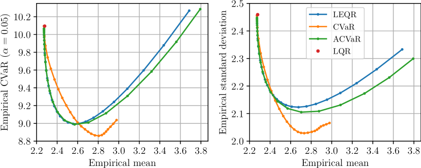
Figure 1: Trade-offs between empirical mean, standard deviation, and $\text{CVaR}_{0.05}$ of the LQR cost for (i) our controller (ACVaR) as $L$ varies, (ii) the LEQR controller as $\gamma$ varies (LEQR), (iii) the exact $\text{CVaR}_{\alpha}$ controller with prior knowledge of the disturbance distribution as $\alpha$ varies (CVaR), and (iv) the LQR controller (LQR). We used the scalar dynamical system $x_{t+1}=x_{t}+u_{t}+w_{t}$ with $R=Q_{f}=1$, $Q=10^{-3}$, $x_{0}=1$, and $N=4$. The disturbance $w_{t}$ is zero-mean Gaussian with unit variance. The parameter ranges were $0.2\leq L\leq 100$, $\frac{\gamma_{\text{c}}}{10}\leq\gamma\leq\gamma_{\text{c}}$, where $\gamma_{\text{c}}$ is the critical $\gamma$ value for LEQR. Each point is the mean of 50,000 trials, where the same schedule of pseudo-random seeds are used across policies. In the limits $L\to\infty$, $\gamma\to 0$, and $\alpha\to 1$ for ACVaR, LEQR, and CVAR_α, respectively, we recover the risk-neutral LQR policy.

7 Concluding Remarks

We took steps toward deriving a scalable upper bound to a distributionally robust, CVaR optimal control problem for linear systems with quadratic costs. CVaR characterizes the (usually abstract) notion of risk as a fraction of worst-case outcomes, which is intuitive and precise. A result from our analysis is a risk-averse controller with intriguing similarities and differences relative to the state-of-the-art.

Potential areas for future work include studying the infinite-horizon case, characterizing the extent to which the upper bound approximation parameterized by $L$ is tight, and elucidating the connections between the choice of $L$ and the maximal covariance $\Sigma$.

Further numerical experiments, potentially with higher-dimensional or more realistic application-specific examples, are needed to ascertain whether the proposed approach may be a superior alternative to LEQR in certain application domains.

References

- [1] T. Başar and P. Bernhard, H∞-Optimal Control and Related Minimax Design Problems: A Dynamic Game Approach, 2nd ed. Birkhauser, 1995.
- [2] K. Zhang, B. Hu, and T. Basar, “On the stability and convergence of robust adversarial reinforcement learning: A case study on linear quadratic systems,” Advances in Neural Information Processing Systems, vol. 33, 2020.
- [3] J. Löfberg, Minimax approaches to robust model predictive control. Linköping University Electronic Press, 2003, vol. 812.
- [4] K. Zhang, B. Hu, and T. Basar, “Policy optimization for linear control with robustness guarantee: Implicit regularization and global convergence,” in Learning for Dynamics and Control. PMLR, 2020, pp. 179–190.
- [5] R. A. Howard and J. E. Matheson, “Risk-sensitive markov decision processes,” Management Science, vol. 18, no. 7, pp. 356–369, 1972.
- [6] D. Jacobson, “Optimal stochastic linear systems with exponential performance criteria and their relation to deterministic differential games,” IEEE Transactions on Automatic Control, vol. 18, no. 2, pp. 124–131, 1973.
- [7] P. Whittle, “Risk-sensitive linear/quadratic/gaussian control,” Advances in Applied Probability, pp. 764–777, 1981.
- [8] ——, Risk-sensitive Optimal Control. Wiley, 1990, vol. 2.
- [9] G. B. Di Masi and L. Stettner, “Risk-sensitive control of discrete-time markov processes with infinite horizon,” SIAM Journal on Control and Optimization, vol. 38, no. 1, pp. 61–78, 1999.
- [10] N. Bäuerle and U. Rieder, “More risk-sensitive markov decision processes,” Mathematics of Operations Research, vol. 39, no. 1, pp. 105–120, 2014.
- [11] R. T. Rockafellar and S. Uryasev, “Conditional value-at-risk for general loss distributions,” Journal of Banking & Finance, vol. 26, no. 7, pp. 1443–1471, 2002.
- [12] J. Kisiala, “Conditional value-at-risk: Theory and applications,” Master’s thesis, School of Mathematics, University of Edinburgh, Aug. 2015.
- [13] S. Samuelson and I. Yang, “Safety-aware optimal control of stochastic systems using conditional value-at-risk,” in American Control Conference, 2018, pp. 6285–6290.
- [14] M. P. Chapman, J. Lacotte, A. Tamar, D. Lee, K. M. Smith, V. Cheng, J. F. Fisac, S. Jha, M. Pavone, and C. J. Tomlin, “A risk-sensitive finite-time reachability approach for safety of stochastic dynamic systems,” in American Control Conference, 2019, pp. 2958–2963.
- [15] A. Majumdar and M. Pavone, “How should a robot assess risk? towards an axiomatic theory of risk in robotics,” in Robotics Research. Springer, 2020, pp. 75–84.
- [16] N. Bäuerle and J. Ott, “Markov decision processes with Average-Value-at-Risk criteria,” Mathematical Methods of Operations Research, vol. 74, no. 3, pp. 361–379, 2011.
- [17] D. P. Bertsekas and S. Shreve, Stochastic Optimal Control: The Discrete-Time Case. Athena Scientific, 1996.
- [18] O. Hernández-Lerma and J. B. Lasserre, Discrete-time Markov control processes: Basic optimality criteria. Springer, 1996, vol. 30.
- [19] R. B. Ash, Real Analysis and Probability. John Wiley & Sons, New York, 1972.
- [20] S. Zymler, D. Kuhn, and B. Rustem, “Distributionally robust joint chance constraints with second-order moment information,” Mathematical Programming, vol. 137, pp. 167–198, 2013.
- [21] P. Gahinet and P. Apkarian, “A linear matrix inequality approach to H control,” International Journal of Robust and Nonlinear Control, vol. 4, no. 4, pp. 421–448, 1994.