Exoplanet Statistics and Theoretical Implications

Abstract

In the last few years, significant advances have been made in understanding the distributions of exoplanet populations and the architecture of planetary systems. We review the recent progress of planet statistics, with a focus on the inner $\lesssim 1\,$AU region of the planetary system that has been fairly thoroughly surveyed by the Kepler mission. We also discuss the theoretical implications of these statistical results for planet formation and dynamical evolution.

1 INTRODUCTION

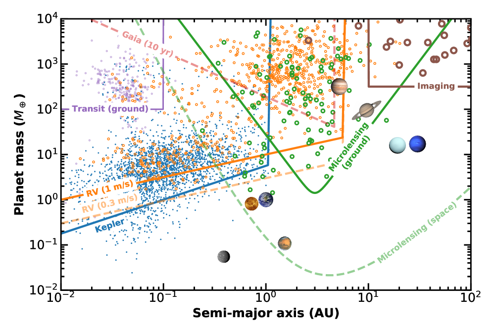
Figure 1: Mass versus semi-major axis of known planets, based on the “Confirmed Planets” list from NASA Exoplanet Archive (Akeson et al., 2013, acquired in September of 2020) and the reliable Kepler planet candidates (see Section 2 for more details). We differentiate with different colors planet detections as well as the approximate sensitivity curves from ground-based transit (purple), Kepler survey (blue), RV surveys (orange), microlensing (green), and direct imaging (brown). The masses of the Kepler detections are estimated from the measured radii according to the Chen & Kipping (2017) mass–radius relation. The sensitivity curve of Kepler is also converted in a similar way from that measured in the radius–period plane (see Figure 2). The sensitivity curve for the 10-yr Gaia astrometry survey is also shown in red, for which we have assumed a Sun-like host at 20 pc and required a 3-$\sigma$ detection over the expected precision. For space-based microlensing, we adopt the sensitivity curve of the microlensing survey that will be performed by the Nancy Grace Roman Space Telescope (formerly known as WFIRST, Penny et al., 2019). Images of the solar system planets from NASA are shown at their corresponding locations.

“Who ordered that?” said the theorist I. Rabi when learning about the unexpected discovery of muons in 1936. Little did particle physicists know that it would only be the beginning of uncovering a puzzling “particle zoo” filled with diverse particles in the next three decades, until revolutionary theoretical insights were developed to classify the elementary particles. Now nearly three decades since the astonishing discovery of a hot Jupiter (Mayor & Queloz, 1995), the “exoplanet zoo” is ever growing – whenever the detection territories grow in breadth or depth, nature appears to be teeming with new species. Theorists working on planet formation and evolution face distinctly different sets of challenges from particle physicists: in the popular paradigm, forming planets from dust grains is a daunting march spanning tens of orders of magnitudes in mass and involves many physical processes that are too complex for first-principle calculations. In hindsight, it should probably be of little surprise that a theory involving such complicated physics, which was anchored by the sole sample of our solar system, would have limited predictive success.

We review the recent progress of planet statistics and identify patterns emerging from the known thousands of exoplanets that cover a broad region of the parameter space (see Figure 1). Robustly identifying patterns in the intrinsic distributions of planets can stimulate and test theories. Conversely, theoretical advances may also beam the searchlight on fresh observational ground, as exemplified by the development of the photoevaporation theory leading to the recent discovery of a “radius valley” (see Section 2.1.4). Since the last Annual Reviews article on exoplanet populations (Winn & Fabrycky, 2015), the field of planet statistics has made significant progress. In particular, the large and homogeneous planet sample from the NASA Kepler mission (Borucki et al., 2010) has provided the best source for statistical studies, but a major shortcoming of the Kepler data was the initial lack of accurate stellar parameters for both the planet hosts and the target stars (i.e., the parent sample). In the last few years, substantial efforts have been dedicated to systematically characterize the Kepler sample and thus unleash its potential for statistical studies. These include asteroseismology (e.g., Chaplin & Miglio, 2013, Van Eylen & Albrecht, 2015), the Gaia data releases (Gaia Collaboration et al., 2016, 2018), follow-up spectroscopic programs such as the LAMOST-Kepler survey (e.g., Dong et al., 2014b, De Cat et al., 2015, Zong et al., 2018) and the California-Kepler Survey (CKS, Petigura et al., 2017, Johnson et al., 2017), as well as many projects of the Kepler Follow-up Observation Program (KFOP, Furlan et al., 2017). Moreover, substantial works to understand the Kepler pipeline detection efficiency and vetting false positives have much improved the reliability of Kepler statistical inference (e.g., Christiansen et al., 2015, Morton et al., 2016). Last but not least, in-depth developments have been recently made to disentangle the intricate observational biases of multi-planet systems. These efforts have made it possible to offer new insights into planet distributions and architectures.

In this review, we first clarify in Sections 1.1 and 1.2 several common confusions in exoplanet statistical studies. Then we discuss planet distributions in the inner ($\lesssim 1\,$AU) and the outer ($\sim 1$–$10\,$AU) regions in Sections 2 and 3, respectively. The former is focused on results from the Kepler mission, and the latter includes updated results from radial velocity (RV) and gravitational microlensing. A brief discussion of the free-floating planets (FFPs) from microlensing is also provided. We focus on planets around $\gtrsim$Gyr-old stars, while planets orbiting young stars found by direct imaging are not discussed (see the review by Bowler 2016). The implications to theories of planet formation and evolution are discussed in Section 4. Finally in Section 5, we summarize and outline the promising directions for future developments.

1.1 On defining and interpreting planet “occurrence rate”

Many statistical studies focus on deriving the intrinsic “occurrence rate” (or the often interchangeably used term “frequency”) of planets. But from one study to another, the same term can carry different meanings. In the following we clarify these different definitions to avoid further misinterpretations.

In most studies, the derived occurrence rate is the average number of planets per star, and we denote it as $\bar{n}_{\rm p}$, which is defined as

$$\bar{n}_{\rm p}\equiv\frac{\rm Total~{}\#~{}of~{}planets}{\rm Total~{}\#~{}of~{}stars}.$$ (1)

Here a planet is restricted to lie within a predefined parameter space, often in the period–radius plane (for the transit method) or the period–mass (or minimum mass $m_{\rm p}\sin{i}$) plane (for the RV method). Similarly, a star is restricted to a star-like target of predefined properties. Since a large fraction of such stars may actually have unresolved stellar companions, the correction for the impact of the stellar binarity can be important for the inference of the planet formation efficiency (see Section 2.5.1).

Another important quantity sometimes referred to as occurrence rate is the fraction of stars with planets $F_{\rm p}$

$$F_{\rm p}\equiv\frac{\rm Total~{}\#~{}of~{}planetary~{}systems}{\rm Total~{}\#~{}of~{}stars}.$$ (2)

Here a planetary system has at least one planet existing in a predefined parameter space. By definition $F_{\rm p}\leq 1$, so it is usually reported as a percentage. However, an occurrence rate reported as a percentage (i.e., “X% of stars have planets”) does not necessarily mean that it is the fraction of stars that are hosts of planets, since $\bar{n}_{\rm p}$ is also frequently reported as a percentage.

[] Frequency of planetsthe average number of planets per star $\bar{n}_{\rm p}$ (Equation 1). Frequency of planetary systemsthe fraction of stars with planets $F_{\rm p}$ (Equation 2). Average planet multiplicitythe average number of planets per planetary system (Equation 3).

To distinguish between the two definitions, we refer to $\bar{n}_{\rm p}$ as the frequency of planets and $F_{\rm p}$ as the frequency of planetary systems. The ratio of the two measures the average number of planets per planetary system (within a predefined parameter space), which we call average planet multiplicity and denote $\bar{m}_{\rm p}$

$$\bar{m}_{\rm p}\equiv\frac{\bar{n}_{\rm p}}{F_{\rm p}}=\frac{\rm Total~{}\#~{}of~{}planets}{\rm Total~{}\#~{}of~{}planetary~{}systems}.$$ (3)

Kepler data suggest that multi-planet systems are common, so usually $\bar{m}_{\rm p}$ is larger than unity, and consequently $\bar{n}_{\rm p}$ and $F_{\rm p}$ substantially differ from each other. They only become similar when the average planet multiplicity $\bar{m}_{\rm p}\rightarrow 1$, which can happen when either a) a category of planets with low intrinsic multiplicity (e.g., short-period giant planets) is concerned, or b) the parameter space of interest is small enough that systems with more than one such planet are rare.

The three quantities, $\bar{n}_{\rm p}$, $F_{\rm p}$, and $\bar{m}_{\rm p}$, are all important for testing theories. To provide a simple example, with only $\bar{n}_{\rm p}$ measured to be unity, it is possible that all stars have one planet ($F_{\rm p}=100\%$ and $\bar{m}_{\rm p}=1$) or that half of the stars have two planets ($F_{\rm p}=50\%$ and $\bar{m}_{\rm p}=2$). These two cases obviously demand different theoretical explanations.

Observationally, the derivations of $\bar{n}_{\rm p}$ and $F_{\rm p}$ have rather different requirements and follow different procedures. It is generally more straightforward to derive $\bar{n}_{\rm p}$, since correcting the detectability of individual planets concerns observables directly measurable from surveys (e.g., planet size and orbital period for transit, assuming that the properties of the stars are known). In contrast, the detectability of a planetary system usually concerns the intrinsic architecture of the system, including the planet multiplicity and distributions of the orbital and physical parameters, many of which may not be directly observable, so the derivation of $F_{\rm p}$ can rely on assumptions of these unknowns. This is especially an issue in transit surveys: the derivation of $F_{\rm p}$ requires assumptions about the mutual inclinations between planets, and different assumptions can lead to fairly different values of $F_{\rm p}$ (see Section 2.2).

In deriving the two frequencies, statistical studies involving multi-planet systems usually treat the planet occurrence as a Poisson process. This may be a reasonable assumption in the derivation of the planet frequency $\bar{n}_{\rm p}$, but it can lead to unreliable results in the derivation of the planetary system frequency $F_{\rm p}$. This Poisson process assumption implies that the presences of individual planets in the same system are independent and that their physical and orbital properties are independent of the properties of other planets or of the host star. As discussed later in this review, such an assumption breaks down in certain circumstances. Below we provide a specific example to demonstrate its impact on the planetary system frequency. The fractions of Sun-like stars with cold giant planets and with planets that Kepler is sensitive to are $10\%$ and $30\%$, respectively. The fraction of such stars with at least one planet in the joint parameter space would be $1-(1-30\%)\times(1-10\%)=37\%$ under the Poisson process assumption. However, this frequency is determined to be $\sim 30\%$ as a result of the strong correlation between the inner and the outer planets (Section 3.2). The correlations (or sometimes anti-correlations) between the occurrences of planets around the same host also suggest that one may not be able to extrapolate a parameterized distribution of the planetary system frequency to a parameter space that is not covered by the data.

A number of studies have reported $F_{\rm p}$ by using the detectability of the first detected (or the most detectable) planet in the system as that of the whole system (e.g., Cumming et al., 2008, Mayor et al., 2011, Fressin et al., 2013, Petigura et al., 2013). This approach does not require assumptions on planet multiplicity or architecture. However, as the detectability of any planet is no greater than the detectability of the system it resides in, this approach typically tends to overestimate $F_{\rm p}$ (Zhu et al., 2018b).

1.2 On inferring the frequency of planets

In this section, we discuss the commonly used methods of inferring the frequency of planets $\bar{n}_{\rm p}$ from a statistical survey of $N_{\star}$ target stars.

A popular method is the so-called inverse detection efficiency method (IDEM), which has been used extensively in the literature, including many influential studies (e.g., Mayor et al., 2011, Howard et al., 2012, Fressin et al., 2013, Petigura et al., 2013, Dressing & Charbonneau, 2013, 2015). For our illustrative survey, the average number of planets per star according to IDEM is

$$\bar{n}_{\rm p}^{\rm IDEM}=\frac{1}{N_{\star}}\sum_{i=1}^{N_{\rm p}}\frac{1}{p_{i}}=\frac{N_{\rm p}}{N_{\star}}\left\langle\frac{1}{p}\right\rangle~{}.$$ (4)

Here $p_{i}$ is the survey detection efficiency of the $i$-th of $N_{\rm p}$ detected planets and $\langle\cdot\rangle$ is the average over all detected planets. IDEM is intuitive, simple to perform, and computationally efficient, as it does not require computing the detection efficiencies of null detections (which are usually the majority of the targets), so it is useful in getting a rough estimate of the underlying frequency. However, this method is not rigorously established in the probability theory and can potentially lead to biased results (Foreman-Mackey et al., 2014, Hsu et al., 2018). Specifically, with a low detection efficiency and a small number of detections, Hsu et al. (2018) found that IDEM often leads to underestimated $\bar{n}_{\rm p}$ since the actual detections typically come from targets with larger-than-average sensitivities. IDEM can also suffer substantial fluctuations because of the inversion of the (typically small) detection efficiency.

An approach with sound statistical basis is modeling planet occurrence as a Poisson process and performing maximum likelihood analysis (e.g., Tabachnik & Tremaine, 2002, Cumming et al., 2008, Gould et al., 2010, Youdin, 2011, Dong & Zhu, 2013, Burke et al., 2015). In a given bin that has $N_{\rm p}$ planet detections, Youdin (2011, see their Section 3.1) and Foreman-Mackey et al. (2014, see their Appendix A) show that the maximum likelihood (ML) estimator for planet frequency is

$$\bar{n}_{\rm p}^{\rm ML}=\frac{N_{\rm p}}{\sum_{j=1}^{N_{\star}}p_{j}}=\frac{N_{\rm p}}{N_{\star}}\frac{1}{\langle p\rangle}=\frac{N_{\rm p}}{N_{\star}^{\rm eff}}~{};\quad N_{\star}^{\rm eff}\equiv N_{\star}\langle p\rangle~{}.$$ (5)

Here $p_{j}$ is the planetary detection efficiency in the bin for the $j$-th star, regardless of whether the star yields any actual planet detection or not, and $N_{\star}^{\rm eff}$ is the effective sample size. Unlike in Equation (4), the average here is performed among all stars in the sample. Compared to IDEM, this method is computationally more expensive, while being statistically superior. It is more robust against fluctuations in the efficiencies of individual detections (as well as null detections) because the averaging is performed on $p$ rather than $1/p$.

Next we elaborate on incorporating the above approach into the Bayesian framework following the simplified Bayesian model of Hsu et al. (2018, see their Appendix B) but with some corrections. The posterior probability distribution of planet frequency $\bar{n}_{\rm p}$ for the statistical sample is given by

$$P(\bar{n}_{\rm p}|N_{\rm p},~{}N_{\star}^{\rm eff})\propto P(N_{\rm p}|\bar{n}_{\rm p},~{}N_{\star}^{\rm eff})P_{\rm pri}(\bar{n}_{\rm p}).$$ (6)

The first term on the right-hand side quantifies the probability (or likelihood) of having the $N_{\rm p}$ detections for a given rate $\bar{n}_{\rm p}$, which under the Poisson process assumption is described by a Gamma distribution . The second term, $P_{\rm pri}(\bar{n}_{\rm p})$, is the prior distribution of $\bar{n}_{\rm p}$. If a conjugate prior is assigned as a Gamma distribution with a shape parameter $\alpha_{0}$ and a rate parameter $\beta_{0}$, the resulting posterior distribution is then a Gamma distribution with the shape parameter $\alpha_{0}+N_{\rm p}$ and the rate parameter $\beta_{0}+N_{\star}^{\rm eff}$

$$P(\bar{n}_{\rm p}|N_{\rm p},~{}N_{\star}^{\rm eff})\propto\bar{n}_{\rm p}^{\alpha_{0}+N_{\rm p}-1}e^{-\bar{n}_{\rm p}(\beta_{0}+N_{\star}^{\rm eff})}.$$ (7)

For a flat prior on $\bar{n}_{\rm p}$, the two parameters are $\alpha_{0}=1$ and $\beta_{0}=0$, respectively. For completeness, the mean and standard deviation of this Gamma distribution posterior are

$$\mu(\bar{n}_{\rm p})=\frac{\alpha_{0}+N_{\rm p}}{\beta_{0}+N_{\star}^{\rm eff}},\quad\sigma(\bar{n}_{\rm p})=\frac{\sqrt{\alpha_{0}+N_{\rm p}}}{\beta_{0}+N_{\star}^{\rm eff}}.$$ (8)

The first expression reduces to the ML estimator of Equation 5 if a log-flat prior on the planet frequency $\bar{n}_{\rm p}$ is assumed (i.e., $\alpha_{0}=\beta_{0}=0$). The expressions given by Equation 8 provide easy-to-use estimates to report when the number of detections is relatively large. However, when small or null detections are involved, the posterior probability distribution is fairly non-Gaussian. It is then more appropriate to report the median value, the 68% credible interval, and/or the 95% upper limit, all of which can be derived from the cumulative posterior probability distribution. It is also worth noting that, in the case of null detections, a meaningful upper limit on $\bar{n}_{\rm p}$ cannot be derived with the log-flat prior because the shape parameter becomes zero and the Gamma distribution is undefined. We show in Section 2.1 an application of the Bayesian approach to derive the frequency of planets in the Kepler parameter space.

2 THE INNER PLANETARY SYSTEM

We review in this section planet statistics in the inner region ($\lesssim 1~{}$AU of Sun-like stars), which is well explored thanks to thousands of planets detected by the RV and transit techniques. We focus on the best statistical probe by far of the inner region—the large and uniform sample from the Kepler mission, which is sensitive to transiting planets with radii $R_{\rm p}$ down to $\sim R_{\oplus}$ and orbital periods $P$ up to $\sim 1~{}$yr (Borucki et al., 2010).

We first derive a clean baseline sample based on the final Kepler data release (DR25, Thompson et al., 2018) and the improved stellar parameters from Berger et al. (2020b). The latter work combines the astrometric measurements from Gaia DR2 (Gaia Collaboration et al., 2018) with the available photometric and spectroscopic information to yield stellar radii with a median uncertainty of $4\%$. Starting from the DR25 planet catalog, we have removed planet candidates with: a) transit signal-to-noise ratio (S/N) below the nominal threshold (S/N$=7.1$), b) NASA Exoplanet Archive disposition flag being false positive, c) the derived planetary radius $R_{\rm p}>20\,R_{\oplus}$, d) the orbital period $P>400\,$days, and e) the best-fit transit impact parameter $b>1$. We restrict to Sun-like stars that are defined as main-sequence stars (as classified by Berger et al. 2018) with effective temperatures between 4700 K and 6500 K. The bulk of this section is about planets around Sun-like hosts, and topics such as correlations with various stellar properties, such as stellar mass, metallicity and binarity, are discussed in Section 2.5.

The baseline sample contains 2,525 planet detections around 98,213 Sun-like stars. Of all the transiting planets, 1451 are found in systems with only one detected transiting planet and the remaining 1074 are from systems with multiple detected transiting planets. The average observed multiplicity rate, namely the average fraction of planets from known multi-planet systems, is $42.5\%$. This is a lower limit on the intrinsic multiplicity rate, as many of the single-planet systems seen in Kepler are likely part of intrinsic multi-planet systems (see details in Section 2.2). The observed transit multiplicity distribution in the sample is

$$(N_{1},~{}N_{2},~{}N_{3},~{}N_{4},~{}N_{5},~{}N_{6},~{}N_{7})=(1451,~{}278,~{}97,~{}37,~{}12,~{}2,~{}1)$$ (9)

and no system has more than seven transiting planets. Figure 2 illustrates the planets in our sample in the radius–period plane. Different multiplicities of transiting planets are shown with different symbols.

2.1 Planet distribution in the radius–period plane

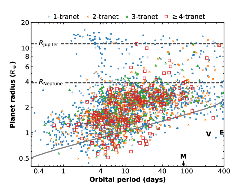
Figure 2: The close-in ($P<400\,$days) Kepler planets in the radius–period plane, with various symbols and colors indicating the observed multiplicity (note that we use the contraction “tranet” to refer to “transiting planet” in the legend). The gray solid curve indicates the median detection efficiency of the planet search pipeline. The solar system planets in the inner region, namely Mercury, Venus, and Earth, are denoted with their first letters. The median precision on the planetary radius is $\sim 7\%$. The radii of the Jupiter and Neptune are shown with horizontal dashed lines, respectively. The radius valley at $\sim 2\,R_{\oplus}$ (see Section 2.1.4) is visible.

With the above statistical sample we derive the planet frequencies in the Bayesian framework of Section 1.2. The parameter space in the radius–period plane is divided into logarithmically equally-spaced cells . In each cell, the number of planet detections, $N_{\rm p}$, is found and the average detection efficiency, $\langle p\rangle$, is computed via

$$\langle p\rangle=\frac{\int_{R_{\rm p,min}}^{R_{\rm p,max}}\int_{P_{\rm min}}^{P_{\rm max}}(R_{\odot}/a)S(P,~{}R_{\rm p})d\ln{P}d\ln{R_{\rm p}}}{\int_{R_{\rm p,min}}^{R_{\rm p,max}}\int_{P_{\rm min}}^{P_{\rm max}}d\ln{P}d\ln{R_{\rm p}}}.$$ (10)

Here $R_{\rm p,min}$, $R_{\rm p,max}$, $P_{\rm min}$, and $P_{\rm max}$ denote the boundaries of the cell, and $R_{\odot}/a$ is approximately the transit geometric probability at semi-major axis $a$ around a Sun-like host. The sensitivity due to survey detection thresholds at a given period and radius, $S(P,~{}R_{\rm p})$, is computed with the KeplerPORTs code, which was first developed in Burke et al. (2015) and further updated for Kepler DR25 (Burke & Catanzarite, 2017a) by incorporating results of transit injection and recovery tests for the final Kepler pipeline (Burke & Catanzarite, 2017b, Christiansen et al., 2020). Updated stellar parameters were used to derive the mean sensitivity curve.

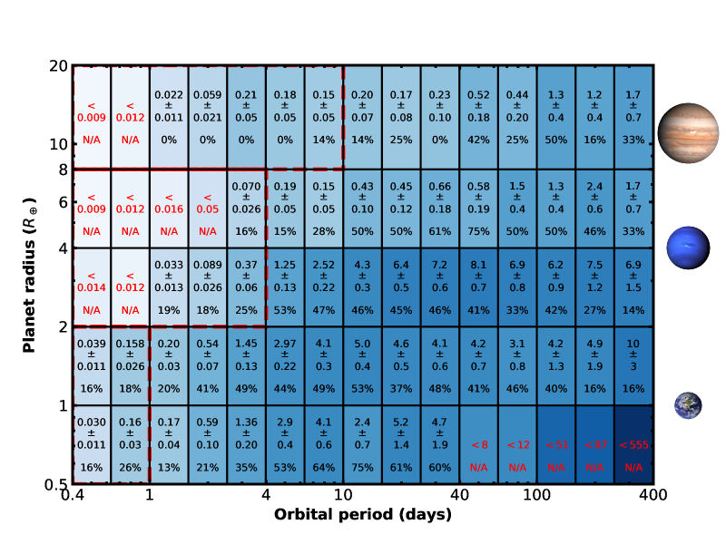
Figure 3: This figure illustrates the planet frequencies ($\bar{n}_{\rm p}$) and the observed multiplicity fractions based on the planet sample in Figure 2. The numbers and error bars are the average number of planets with periods and radii within the given cell per 100 Sun-like stars. If there are less than three detections found within the cell, then the $95\%$ upper limit is reported instead. These upper limits are highlighted in red. The fraction in each cell denotes the observed multiplicity fraction, namely the fraction of planets in that cell found to reside in multi-planet systems. We use “N/A” for cells with less than three detections. The red dashed lines mark the regions corresponding to hot Jupiters, hot Neptune “desert,” and USPs.

We adopt a flat prior on $\bar{n}_{\rm p}$, and its posterior distribution is then described by the Gamma distribution of Equation 7 with $\alpha_{0}=1$ and $\beta_{0}=0$. For cells with $\leq 2$ detections we report the 95% upper limits, whereas for the rest the means and the standard deviation given by Equation 8 are reported as the measurements and associated uncertainties, respectively. We have verified that the deviation between the mean and the median is substantially smaller than the uncertainty for all relevant cells.

The derived planet frequency map is shown in Figure 3. For cells with more than two detections, we also indicate the observed multiplicity rate of planets in the cell. Again, these multiplicity rates represent the lower limits on the fraction of planets in those cells that reside in multi-planet systems. We summarize several key results below:

• The integrated planet frequency is $\bar{n}_{\rm p}=1.23\pm 0.06$ for planets with radii in the range 1–$20\,R_{\oplus}$ and orbital periods up to $400\,$days. This is broadly consistent with results from previous studies (e.g., Fressin et al., 2013, Petigura et al., 2018, Hsu et al., 2019). As stressed in Section 1.1, statistical analyses like this one do not yield the fraction of stars with planets $F_{\rm p}$, as the impact of the multiplicity and the mutual inclination has not been taken into account (see Section 2.2).

• As it has been clear since the earliest Kepler statistical studies, there are generally many more small planets with radii $R_{\rm p}\lesssim 4\,R_{\oplus}$ than larger ones, for orbital periods $P<400\,$days. Planet frequencies tend to increase from the upper left (large $R_{\rm p}$ and small $P$) toward the lower right (small $R_{\rm p}$ and large $P$). In other words, the intrinsic radius distribution is dependent on the orbital period (e.g., Dong & Zhu, 2013, Foreman-Mackey et al., 2014, Hsu et al., 2018). There exist some local regions where the general trends break down, such as the radius valley (see Section 2.1.4).

• Sub-Earths ($R_{\rm p}<1\,R_{\oplus}$) and Earth-sized planets in Earth-like orbits are not well probed by Kepler, and thus estimates of their frequencies are most susceptible to the uncertainties of survey sensitivity estimates. As a result, there remain large discrepancies on their intrinsic frequencies in the literature (see Table 2 of Winn & Fabrycky 2015 and Figure 17 of Burke et al. 2015).

• Kepler planets commonly reside in multi-planet systems in most parts of the radius–period plane, with some notable exceptions such as the hot Jupiter region (Steffen et al. 2012; see Section 2.1.1 for more discussion). The intrinsic multiplicity rates are likely higher than the observed multiplicity rates shown in Figure 3. We defer to Section 2.2 for further discussions.

The above method to derive the planet frequency $\bar{n}_{\rm p}$ is non-parametric. An alternative approach employs a parameterized planet distribution function and then constrains the associated parameters. The parametric approach has been widely used in statistical studies of various detection techniques, including transit (e.g., Youdin, 2011, Howard et al., 2012, Dong & Zhu, 2013, Burke et al., 2015), RV (e.g., Tabachnik & Tremaine, 2002, Cumming et al., 2008), and microlensing studies (e.g., Gould et al., 2010, Suzuki et al., 2016, Clanton & Gaudi, 2016). It is also commonly used in simulations of generating synthetic planetary systems (e.g., Mulders et al., 2018, He et al., 2019). The commonly adopted planet distribution function is separable between the orbital period (or semi-major axis) and the planetary radius (or mass)

$$\frac{d^{2}N}{d\ln{P}d\ln{R_{\rm p}}}\propto\frac{dN}{d\ln{P}}\frac{dN}{d\ln{R_{\rm p}}}.$$ (11)

The distributions of the orbital period and the planetary radius are usually parameterized as power laws or broken power laws. The use of such a separable function implicitly assumes that the period (radius) distribution is independent of the planetary radius (period). As discussed above, such an assumption is not valid for the inner planetary system. It is likely not valid for planet distributions in other regions of the parameter space, either. The implications of this failure on the derived occurrence rates from the parametric method and on the theoretical interpretations of the underlying population have not been fully explored.

In what follows, we provide brief discussions about selected regions in the radius–period plane.

2.1.1 Hot Jupiters

As the first type of exoplanets found around solar-type stars (Mayor & Queloz, 1995), hot Jupiters ($8\,R_{\oplus}<R_{\rm p}<20\,R_{\oplus}$ and $P<10\,$days) remain interesting and exciting targets for both observational and theoretical purposes. Here we only review the occurrence and multiplicity rates of hot Jupiters in the current context and refer interested readers to the recent review by Dawson & Johnson (2018) for more in-depth discussions about the hot Jupiter population.

There is a long-standing discrepancy between the hot Jupiter frequency inferred from RV and transit surveys (e.g., Gould et al. 2006a, Wright et al. 2012; see Table B9 of Santerne et al. 2016 for an incomplete list). For example, our statistical sample yields a rate of $0.62\pm 0.09\%$, which is in good agreement with previous studies of the hot Jupiter frequency in the Kepler field (e.g., Howard et al., 2012, Fressin et al., 2013, Santerne et al., 2016), whereas the RV surveys of stars in the Solar Neighborhood report rates that are typically a factor of $\sim$2 higher ($0.9$–$1.2\%$; Mayor et al. 2011, Wright et al. 2012). It was suggested that the discrepancy could be caused by the different stellar properties, such as age, metallicity, and binary fraction, between the RV and transit samples. This has been tested by several follow-up studies of the Kepler sample. The Kepler stars are only slightly sub-solar on average ($\left\langle{\rm[Fe/H]}\right\rangle_{\rm Kepler}\approx-0.04$; Dong et al. 2014b), and their metallicity differences with the RV targets ($\left\langle{\rm[Fe/H]}\right\rangle_{\rm RV}\approx 0.0$) seem to be too small to fully account for the discrepancy even given the steep dependence of hot Jupiter frequency with metallicity (Guo et al., 2017). The unresolved binaries are also unlikely to substantially change the hot Jupiter frequency in the Kepler sample (Bouma et al., 2018). However, because RV surveys preferentially exclude close ($\sim 1$–$50\,$AU) stellar binaries from their sample, this discrepancy in hot Jupiter frequencies between transit and RV surveys can potentially be resolved if the formation of hot Jupiters are suppressed in such close binary systems (Moe & Kratter, 2019). Searching for stellar companions of transiting hot Jupiters (e.g., Ngo et al., 2016) and making comparisons with field stars is a promising way to further test this possibility.

As shown in Figure 2, one out of the 49 hot Jupiters in our statistical sample, Kepler-730b, has a nearby small planet companion (Zhu et al., 2018a, Cañas et al., 2019). As of writing, only two other hot Jupiters, WASP-47b (Becker et al., 2015) and TOI-1130c (Huang et al., 2020) are known to share the same property. Our statistical sample suggests that $\sim 2\%$ ($<9.7\%$, $95\%$ upper limit) of hot Jupiters have nearby ($\lesssim 20$ days), small ($\sim$1–$4\,R_{\oplus}$) and nearly coplanar companions (see also Steffen et al. 2012 for the constraint on non-coplanar companions). This low multiplicity rate of hot Jupiters supports the general idea that most of them have undergone some large-scale migrations to arrive at current locations (e.g., Lin et al., 1996, Rasio & Ford, 1996a, Weidenschilling & Marzari, 1996). We refer to Dawson & Johnson (2018) for more in-depth discussions on this topic.

2.1.2 Hot Neptune “desert”

The region $P\lesssim 4\,$days and $2\,R_{\oplus}\lesssim R_{\rm p}\lesssim 8\,R_{\oplus}$ lands in the so-called hot Neptune (or sub-Jovian) “desert” (e.g., Szabó & Kiss 2011, Beaugé & Nesvorný 2013, Mazeh et al. 2016 and references therein), which is considered underpopulated, especially when inspecting mixed planet samples found in surveys with different detection sensitivities (e.g., ground-based transits and Kepler). This “desert” is however not that barren: the total planet frequency enclosed in the above region is $0.61\pm 0.07\%$ from our statistical analysis (see Figure 3), making this hot Neptune “desert” similarly populated as the hot Jupiter region (see also Dong et al., 2018). While the above frequency is derived for a rectangular region in the radius–period plane, it is worth noting that the boundaries of this “desert” region are better described as a triangle and extend out to $5$–$10$ d in $m_{\rm p}$ vs. $a$ and $R_{\rm p}$ vs. $P$ planes (see Figure 1 and Figure 4 of Mazeh et al. 2016). Dong et al. (2018) found that the frequency of planets inside this region depends on the host star metallicity in a way similar to the frequency of hot Jupiters, and they dubbed this population as “Hoptunes” (rather than “hot Neptunes”) to reflect that not all of them were known Neptune-like physically. Out of our baseline sample of 61 planets in this region, 14 are observed to have planetary companions, and the periods for majority of these companions are within 10 d. The observed multiplicity rate is thus $23\%$, which is lower than the Kepler average while higher than that of hot Jupiters (see also Dong et al., 2018). We refer to Dawson & Johnson (2018) for more discussions on the connection of this population with close-in Jupiters and related theoretical implications.

A number of theories have been proposed to explain the formation of planets in this region (e.g., Kurokawa & Nakamoto, 2014, Matsakos & Königl, 2016, Lundkvist et al., 2016, Bailey & Batygin, 2018, Owen & Lai, 2018). The leading explanations of its triangular boundaries invoke photoevaporation (see more discussion in Section 2.1.4) and tidal effects following the high-eccentricity migration. The upper boundary is best explained as the tidal disruption barrier for gas giants following their high-eccentricity migrations (Matsakos & Königl, 2016, Owen & Lai, 2018). More massive planets can be tidally circularized closer to the star without tidal disruption, resulting in the negative slope of the upper boundary. It has been proposed that the same mechanism also produces the lower boundary, with the positive slope resulting from a mass–radius relation of small planets that is different from the relation of giant planets (Matsakos & Königl, 2016). However, this mechanism may not be able to explain the planets that are in or near the “desert” region and reside in multi-planet systems. An alternative theory, proposed by Owen & Lai (2018), suggests that the lower boundary is better explained by the photoevaporation of highly irradiated planets, and that the positive slope results from the fact that the photoevaporation mechanism is more effective if the planet is closer to the host star. There has been a growing interest of planets in this region with the TESS mission (e.g., Armstrong et al., 2020, Burt et al., 2020), and the follow-up studies of such planets will soon allow for a better understanding of their physical properties and formation mechanisms.

2.1.3 Ultra-short-period planets

Planets with radii between $0.5$–$2\,R_{\oplus}$ and periods $P\lesssim 1\,$d, known as ultra-short-period planets (USPs), represent a rather extreme planet population. The period threshold for USPs at one day corresponds to an equilibrium temperature $\sim 2000\,$K for a Sun-like host, which is hot enough to sublimate dust grains. Below we briefly summarize several key properties of USPs and refer interested readers to the recent comprehensive review by Winn et al. (2018) for more discussions about this extreme planet population.

Our statistical analysis yields $\bar{n}_{\rm p}=(0.39\pm 0.04)\%$ for USPs. This is in general agreement with the result of Sanchis-Ojeda et al. (2014), whose specialized pipeline yields $\bar{n}_{\rm p}=(0.51\pm 0.07)\%$ for planets with radii in the range $0.8$–$2\,R_{\oplus}$ and $P<1\,$d. Out of the 81 USPs in our sample, 16 are found with outer planetary companions, indicating an observed multiplicity rate of $20\%$. The true multiplicity rate is probably much higher, since USPs can be largely misaligned relative to the outer planetary companions (Dai et al., 2018, Petrovich et al., 2019). In 13 of the 16 multi-planet systems involving USPs, the closest outer companion has $P_{\rm c}\lesssim 10\,$d, and the USP is usually farther apart in terms of the period ratio from the rest of the planets in the same system (see also Steffen & Farr 2013).

The highly irradiative environment at sub-day orbit implies that USPs are unlikely to have formed in situ. Partially because of the comparable rates between hot Jupiters and USPs, it had been suggested that USPs could be the surviving cores of tidally disrupted hot Jupiters (Jackson et al., 2013), but this was not supported by several pieces of evidence including the lack of strong host metallicity dependence (Winn et al., 2017) and the relatively high multiplicity rate compared to hot Jupiters. A more plausible scenario is that the USPs have arrived at their current locations without losing much of their initial mass. One way of achieving this is the gradual decay of the orbit due to the tidal dissipation within the host star (Lee & Chiang, 2017). Alternatively, the proto-USP planet may have been sent to an eccentric (and misaligned) orbit following the dynamical interactions with other planets in the system, and then the orbit decays and circularizes due to the tidal dissipation within the planet (Schlaufman et al., 2010, Petrovich et al., 2019, Pu & Lai, 2019). This latter model sees its support in the relatively large mutual inclinations of USPs (Dai et al., 2018). Additionally, in order for the tidal inspiral model to produce USPs, the tidal dissipation in USP hosts needs to be efficient, but the population analysis on stellar kinematic ages seems to suggest otherwise (Hamer & Schlaufman, 2020).

2.1.4 Radius valley

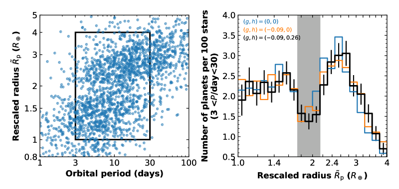
Figure 4: (a) The zoom-in view of the Kepler planets in our sample centered at the radius valley. The $y$-axis shows the rescaled radius $\tilde{R}_{\rm p}\equiv R_{\rm p}(P/{10\,\rm days})^{-g}(M_{\star}/M_{\odot})^{-h}$ (see Equation 12) and we adopt the best-fit $g=-0.09$ (Van Eylen et al., 2018) and $h=0.26$ (Berger et al., 2020a). The black box marks the boundary within which planets are used to derive the intrinsic radius distribution. (b) The intrinsic distribution of the rescaled radius $\tilde{R}_{\rm p}$. The radius gap, highlighted in the gray band, is most prominent when both period and stellar mass dependences are taken into account.

An important discovery in the field of exoplanet in recent years is the radius valley, which refers to a region in the radius–period plane at radii $R_{\rm p}\sim 2\,R_{\oplus}$ and periods between $\sim$3–$30\,$days (Fulton et al., 2017, Van Eylen et al., 2018, Fulton & Petigura, 2018). This radius valley is visible in our statistical sample (see Figure 2). The position of the valley in radius is reported to decrease with the orbital period (Van Eylen et al., 2018) and increase with the stellar mass (Wu, 2019, Berger et al., 2020a). The two dependences can be parameterized as

$$\frac{R_{\rm p}}{R_{\rm p}^{\rm valley}}=\left(\frac{P}{10\,\rm days}\right)^{g}\left(\frac{M_{\star}}{M_{\odot}}\right)^{h}.$$ (12)

The valley position at orbital period $P=10\,$days and host mass $M_{\star}=M_{\odot}$ is found to be $R_{\rm p}^{\rm valley}=1.9\pm 0.2\,R_{\oplus}$ and the slope quantifying the period dependence is $g=-0.09^{+0.02}_{-0.04}$ (Van Eylen et al., 2018). The slope quantifying the stellar mass dependence is $h=0.26^{+0.21}_{-0.16}$ (Berger et al., 2020a). With the above relation one can then highlight the radius valley by rescaling the radius to $\tilde{R}_{\rm p}\equiv R_{\rm p}(P/{10\,\rm days})^{-g}(M_{\star}/M_{\odot})^{-h}$. Figure 4a illustrates our sample in this rescaled radius (with $g=-0.09$ and $h=0.26$) vs. orbital period plane. We also show the intrinsic distribution of the rescaled radius in Figure 4b for planets with $\tilde{R}_{\rm p}$ in the range $1$–$4\,R_{\oplus}$ and $P$ in the range $3$–$30\,$days. Our choice of the period upper boundary is motivated by Figure 2: beyond $\sim 30\,$days the number of detections in the relevant region and thus the statistical power drops significantly. The peak-to-dip contrast in our “radius” distribution is not as significant as that shown in Fulton et al. (2017) and Fulton & Petigura (2018). In particular, our rescaled radius distribution does not show an obvious single peak at $\tilde{R}_{\rm p}<R_{\rm p}^{\rm valley}$. We have tried with the same period range as used in those studies and confirm that our specific choice of the period range is not the cause of this difference. One possible reason is the different statistical methods used to infer the occurrence rate: As discussed in Section 1.2, the IDEM approach used in Fulton et al. (2017) and Fulton & Petigura (2018) tends to underestimate the occurrence rates at low sensitivity regions ($R_{\rm p}\sim R_{\oplus}$). The fact that the radius distribution does not seem to decrease at sub-Earth sizes suggests the presence of many undiscovered sub-Earths. The broader radius distribution may also imply that the planetary mass distribution is not as narrowly peaked as some previous studies inferred (e.g., Wu, 2019).

The leading theory for the radius valley is the atmospheric evaporation driven by high-energy photons from the host star (photoevaporation; Owen & Wu, 2013, Lopez & Fortney, 2013, Owen & Wu, 2017). In fact, the existence of the radius valley at approximately the discovered position had been predicted years before its discovery (Owen & Wu 2013, Lopez & Fortney 2013; see a historic overview in Owen 2019), which is exceptional in exoplanetary science. The photoevaporation of the atmosphere is thought to mostly take place during the early ages of the system when the star emits a higher fraction of its total luminosity at high energy ($\lesssim 100\,$Myr; e.g., Jackson et al. 2012, Tu et al. 2015, but also see King & Wheatley 2021). For close-in ($\sim 3$–$30\,$days) planets with core masses of a few $M_{\oplus}$, the high-energy radiation is sufficient to unbind the entire hydrogen/helium atmosphere if its initial mass fraction is below some critical value (a few percent; Owen & Wu 2017). The radius valley thus emerges, separating planets with and without extended atmospheres (Owen & Wu, 2013, Lopez & Fortney, 2013, Owen & Wu, 2017). The observed period and stellar mass dependences can also be well explained by photoevaporation. As the orbital period increases and/or the host mass decreases, the amount of high-energy radiation the planet receives decreases and thus the valley moves to smaller radii (Owen & Wu, 2017, Wu, 2019). We refer interested readers to Owen (2019) for a comprehensive review on the photoevaporation mechanism.

According to the photoevaporation theory, the properties (e.g., location and shape) of the radius valley depend on the underlying planetary properties, especially distributions of the core mass, core composition, and atmospheric mass fraction (Owen & Wu, 2013, Lopez & Fortney, 2013). Therefore, the observed radius valley opens up a venue to statistically infer the properties of close-in low-mass planets at birth (Owen & Wu, 2017, Jin & Mordasini, 2018, Wu, 2019, Rogers & Owen, 2020). Assuming that photoevaporation is the underlying mechanism, these studies collectively point to a typical core mass of a few $M_{\oplus}$, a core composition similar to that of the Earth (i.e., rich in silicate/iron and poor in water/ice), and a typical atmosphere mass fraction at birth of a few percent. These inferred properties have important implications to the formation and migration history of these close-in planets (see Section 4).

While photoevaporation has seen its success in predicting and explaining the radius valley, alternative theories exist that can also explain the observed valley (e.g., Ginzburg et al., 2018, Lee & Connors, 2020), of which the core-powered mass-loss mechanism is considered the main competing theory. Unlike photoevaporation, the energy source for atmosphere stripping in core-powered mass-loss mechanism is the internal luminosity of the cooling core, and this process is expected to operate on much longer timescales ($\sim$ Gyr) (Ginzburg et al., 2018). The observed period and stellar mass dependences of the radius valley (Equation 12) are also consistent with this mechanism (Gupta & Schlichting, 2019, 2020). Similar to photoevaporation, core-powered mass-loss mechanism also supports that the close-in low-mass planets have predominantly rocky cores with low water-ice fractions (Gupta & Schlichting, 2019).

Attempts have been made to identify which of the two mechanisms discussed above is more responsible for the observed features. These studies made use of either the different stellar mass or age dependences of the two mechanisms (e.g., Hirano et al., 2018, Berger et al., 2020a). However, the currently available data provide no conclusive result to distinguish between the two. Larger samples and/or more precise measurements of stellar properties will be needed.

2.2 Mutual inclinations and the intrinsic multiplicity

The mutual inclination distribution of planets in multi-planet systems conveys important information on the formation and dynamical evolution of planetary systems. However, currently employed detection techniques are usually incapable of directly measuring mutual inclinations. This is particularly true for RV and microlensing. The transit technique is strongly biased toward (nearly) coplanar systems. Nevertheless, advancements have made it possible to statistically infer the mutual inclination distribution from the Kepler data.

The key issue in constraining the mutual inclination distribution with transit is the strong degeneracy with the intrinsic multiplicity (e.g., Lissauer et al., 2011, Tremaine & Dong, 2012). Specifically, with the observable multiplicity function of transit alone one cannot distinguish between high-multiplicity systems with large mutual inclinations and low-multiplicity systems with small mutual inclinations. We therefore combine mutual inclinations and intrinsic multiplicity in the same discussion.

Before discussing the statistically inferred mutual inclinations, we briefly overview a handful of systems with measured large mutual inclinations. By combining HST astrometry and ground-based RV measurements, McArthur et al. (2010) measured the mutual inclination between two of the three planetary companions in the Upsilon Andromeda system to be about $30^{\circ}$. Mills & Fabrycky (2017) performed photo-dynamical modeling of the transit timing variation (TTV) and transit duration variation (TDV) signals of the Kepler-108 system and found the mutual inclination to be $\Delta I=24_{-8}^{+11}\,{}^{\circ}$ between the two transiting planets. The pi Mensae system, which hosts a long-period giant planet and a TESS transiting super Earth (Huang et al., 2018, Gandolfi et al., 2018), is reported to have significant mutual inclinations ($\sim 30$–$150^{\circ}$) from joint analyses of the Hipparcos and Gaia DR2 astrometry (Xuan & Wyatt, 2020, Damasso et al., 2020, De Rosa et al., 2020). Additionally, some USP systems have also been determined to have large mutual inclinations (e.g., Dai et al., 2018). More planetary systems with large mutual inclinations are expected to be found in the following years, especially with Gaia’s capability to determine the 3D orbital configurations (Perryman et al., 2014).

2.2.1 The weighted transit duration method

A popular method to statistically infer the mutual inclination of Kepler muti-planet systems makes use of the ratio of transit chord lengths (Steffen et al., 2010)

$$\xi\equiv\frac{T_{\rm in}P_{\rm in}^{-1/3}}{T_{\rm out}P_{\rm out}^{-1/3}}=\sqrt{\frac{(1+r_{\rm in})^{2}-b_{\rm in}^{2}}{(1+r_{\rm out})^{2}-b_{\rm out}^{2}}}~{}.$$ (13)

The subscripts “in” and “out” denote values of the inner and the outer transiting planets, respectively. Here $T$ measures the time from the first to the last contact points of transit, $r$ is the planet-to-star radius ratio, and $b$ is the transit impact parameter. As both $T$ and period $P$ are precisely measured from transit data (Seager & Mallén-Ornelas, 2003), the parameter $\xi$ is well determined from observations. The last expression in Equation 13 is used to construct the $\xi$ distribution from models with assumed mutual inclination distributions. When two transiting planets are exactly coplanar, the ratio $b_{\rm in}/b_{\rm out}=a_{\rm in}/a_{\rm out}=(P_{\rm in}/P_{\rm out})^{2/3}$ is precisely measured and thus the parameter $\xi$ only concerns one poorly constrained fiducial parameter (either $b_{\rm in}$ or $b_{\rm out}$, since both $r_{\rm in}$ and $r_{\rm out}$ are reasonably well measured). The distribution of $\xi$ for coplanar systems is thus expected to narrowly peak at unity. In practice, the observed distribution is not so narrow, because of the introduction of the mutual inclination (see Figure 5a). Applying this weighted transit duration method to large samples of Kepler planet pairs, Fang & Margot (2012) and Fabrycky et al. (2014) found that the mutual inclinations between transiting planets in the Kepler multi-planet systems could be well described by a Rayleigh distribution with a dispersion of a few degrees ($\lesssim 3$–$5^{\circ}$). This has been frequently interpreted as multi-planet systems being nearly coplanar. However, with the use of only transiting planet pairs, which preferentially have small mutual inclinations, the weighted transit duration method cannot well determine the higher end of the mutual inclination distribution. As an extreme case, even the isotropic distribution of orbital inclinations cannot be reliably ruled out with the use of transit data alone (Tremaine & Dong, 2012).

2.2.2 “Kepler dichotomy”

To recover the true mutual inclination distribution, one needs to break its strong degeneracy with intrinsic multiplicity. The first attempt was carried out by Lissauer et al. (2011). The authors tried different functional forms for the intrinsic multiplicity distribution (uniform, Poisson, and exponential) as well as for the mutual inclination distribution (uniform and Rayleigh; see also Sandford et al. 2019). By modeling the intrinsic multiplicity as a uniform (or Poisson) distribution and the mutual inclination as a Rayleigh distribution, Lissauer et al. (2011) were able to find matches to all observed transit multiplicities except the transit singles. Specifically, their models would under-predict the number of systems with only one transiting planets by nearly $50\%$. This signals the failure of their simplified model. Nevertheless, this feature was picked up by many others and phrased as the evidence for two distinct populations of planetary systems (the so-called “Kepler dichotomy”): In one population planetary systems have small mutual inclinations and relatively compact configurations, whereas in the other population planetary systems have either only one planet or at least two largely mutually inclined planets (e.g., Johansen et al., 2012, Ballard & Johnson, 2016, Mulders et al., 2018, He et al., 2019). Taking the Kepler sample as a whole, in terms of distributions of many properties of stars (e.g., stellar mass, metallicity) and planets (e.g., period), transit singles and transit multis are statistically consistent with being drawn from the same parent population (e.g., Xie et al., 2016, Munoz Romero & Kempton, 2018, Zhu et al., 2018b, Weiss et al., 2018a), suggesting that they probably have the same origin.

While modeling the mutual inclination as a Rayleigh distribution (or more generally, Fisher distribution; Tremaine & Dong 2012, Zhu et al. 2018b) seems a reasonable choice (see also Tremaine, 2015), the proper functional form for the intrinsic multiplicity distribution remains an open question. Nevertheless, it is certainly oversimplified to assume that all planetary systems have the same number of planets (e.g., Ballard & Johnson, 2016, Mulders et al., 2018). Having a Poisson distribution for the intrinsic multiplicity (e.g., Lissauer et al., 2011, Zink et al., 2019, Sandford et al., 2019, He et al., 2019) is likely not justified, either. The underlying assumption behind the Poisson distribution is that occurrences and properties of individual planets around the same host are independent from each other. While it has not been proved invalid for Kepler planets, there is emerging evidence that the presence and properties of planets inside the same system may be correlated due to the shared formation environment and/or host properties (see Sections 1.1, 2.4 and 2.5). Furthermore, the exponential or power-law (i.e., Zipfian distribution; Sandford et al. 2019) forms can be securely ruled out. These distributions predict overly abundant intrinsic single-planet systems, which is not supported by TTV observations (see below).

Given the strong degeneracies, disentangling the intrinsic multiplicity function and the mutual inclination distribution therefore requires external information. To this end, Tremaine & Dong (2012) developed a general statistical framework to account for observational biases of different techniques. Applying their method to planetary systems found by Kepler and RV, Tremaine & Dong (2012) found that the mean mutual inclination dispersion, which was assumed to be the same for all multiplicities, should be $\lesssim 5^{\circ}$ and that the intrinsic multiplicity function could not be constrained. See Figueira et al. 2012 for a different attempt in combining Kepler and RV data.

Tremaine & Dong (2012) also pointed out an observational feature that was difficult for their models to explain. As originally noticed by Ford et al. (2011), the fraction of systems showing TTV signals does not seem to vary significantly with the transit multiplicity, except perhaps for very high ($\geq 4$) multiplicities (see also Xie et al. 2014). A similar feature also shows up in later large and uniform TTV searches, which consistently found that nearly half of the TTV detections were from systems with only one transiting planets (Holczer et al., 2016, Ofir et al., 2018). This indicates that planets in transit singles have almost the same probability to show TTV signals as planets in transit multis.

2.2.3 Multiplicity-dependent mutual inclinations

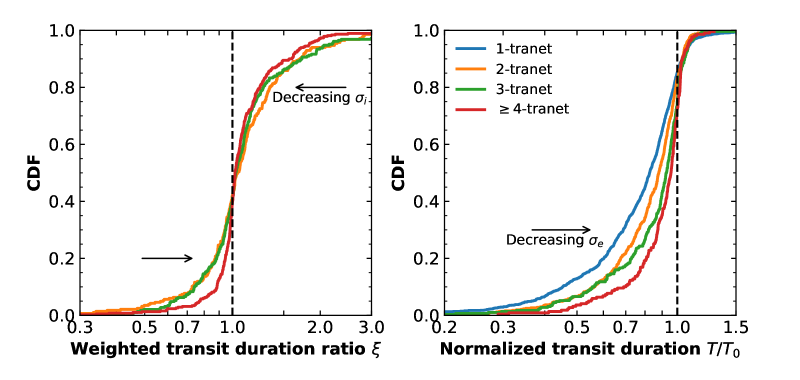
Figure 5: (a) The cumulative distribution functions (CDFs) of the weighted transit duration ratio, $\xi$ (Equation 13), for different transit multiplicities. Larger transit multiplicities tend to have narrower $\xi$ distributions, suggesting smaller mutual inclination dispersions $\sigma_{i}$. (b) The CDFs of the normalized transit duration, $T/T_{0}$ (Equation 15), for different transit multiplicities. Here $T_{0}$ is the transit duration for a circular and coplanar orbit. Larger transit multiplicities have narrower $T/T_{0}$ distributions, indicating smaller eccentricity dispersions $\sigma_{e}$.

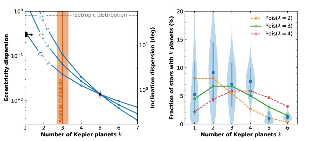
Figure 6: (a) Distributions of eccentricity and mutual inclination dispersions as functions of the intrinsic multiplicity. Here Kepler window is roughly the region above the gray curve in Figure 2. The relation $\sigma_{e}=\sigma_{i}$ is assumed (see Section 2.3.2). The $\zeta$ parameter quantifies the strength of the correlation with the intrinsic multiplicity (Equation 14). The orange band denotes the inferred average multiplicity $\bar{m}_{\rm p}$ for Kepler systems. The eccentricity dispersion inferred from transit singles (i.e., $k\geq 1$) and the mutual inclination dispersion constraint from systems with five Kepler transiting planets are shown as black squares. (b) The inferred intrinsic multiplicity vector and the associated probability distribution functions. The fraction of Sun-like stars with more than seven planets in the Kepler window is limited to $<2.2\%$ ($95\%$ upper limit). The medians and the $16$–$84\%$ ranges of individual components are denoted with squares and error bars, respectively. Poisson distributions with different values of mean parameter $\lambda$ are shown for references. Both plots are adapted from Zhu et al. (2018b).

The assumption that the mutual inclination distribution is independent of the intrinsic multiplicity may not be valid. With all else being equal, the critical mutual inclination for long-term instability is probably dependent on the number of planets in the system (e.g., Pu & Wu 2015; see also Section 2.4.2). Observationally, one also finds that the distribution of the $\xi$ parameter appears statistically different for different transit multiplicities. As shown in Figure 5a, lower transit multiplicities have broader $\xi$ distributions that are suggesting larger mutual inclinations (see also He et al. 2020).

Zhu et al. (2018b) introduced the following relation between the mutual inclination dispersion, $\sigma_{i}$, and the intrinsic multiplicity (within Kepler window), $k$,

$$\sigma_{i}(k)=0.8^{\circ}\left(\frac{k}{5}\right)^{\zeta}~{}.$$ (14)

They applied the statistical framework of Tremaine & Dong (2012) and combined the transit and TTV statistics to infer the intrinsic multiplicity and mutual inclination distributions. TTV, as a detection technique (Agol et al., 2005, Holman & Murray, 2005), applies to the same population of planetary systems as transit, and thus the combination of TTV and transit is free from many assumptions and selection biases (compared to the use of RV; e.g., Tremaine & Dong 2012). Zhu et al. (2018b) found that the intrinsic multiplicity and the mutual inclination dispersion should be strongly correlated, with $-4<\zeta<-2$ at the $2\,\sigma$ confidence level (see Figure 6a for an illustration). In other words, systems with fewer planets are dynamically hotter. This result also points to large mutual inclinations ($\gtrsim 10^{\circ}$) for 2-planet and 3-planet systems. A recent work by He et al. (2020) found a qualitatively similar (although statistically different) result with a best-fit $\zeta=-1.7$ from modeling a collection of Kepler statistics (including transit multiplicities, the period distribution, period ratio distribution, etc) and imposing the angular momentum deficit (AMD) stability criterion (Laskar, 1997, Laskar & Petit, 2017) in simulated planetary systems. It is also worth noting that such a relation is steeper than the similar relation inferred from RV eccentricities (Limbach & Turner, 2015), ergodic models (Tremaine, 2015), or the extrapolations of the empirical stability boundary (e.g., Pu & Wu, 2015).

Zhu et al. (2018b) also reported constraints on the intrinsic multiplicity vector, which is reproduced in Figure 6b. Although the individual components of the multiplicity vector are not well constrained, the summed fraction is well measured to be $30\pm 3\%$ and does not rely on many assumptions like the other measurements do (see Section 5.1 of Zhu et al. 2018b; see also Section 1.1). The resulting average multiplicity in the Kepler parameter space is $\bar{m}_{\rm p}=3.0\pm 0.3$. This serves a lower bound on the average multiplicity in the inner ($\lesssim 1\,$AU) region, as smaller planets below the detection threshold of Kepler are unconstrained.

2.3 Eccentricity distribution

Similar to mutual inclinations, orbital eccentricities also provide important information on the formation and dynamical evolution of planetary systems. Here we focus on the eccentricity results from the Kepler sample. Readers can find discussions about eccentricities from RV in the Section 3.1 of Winn & Fabrycky (2015).

The majority of the eccentricity measurements of individual Kepler planets were made through modeling the TTV and TDV signals (e.g., Lithwick et al., 2012, Wu & Lithwick, 2013, Hadden & Lithwick, 2014, 2017). These studies have found that the eccentricities of Kepler planets in near-resonance pairs are typically small, with a Rayleigh dispersion of up to a few percent. However, the planets selected for such dynamical modelings are probably a biased sample, and thus the derived eccentricity distribution may not be representative of the more general population.

2.3.1 The transit duration method

The transit duration (between the first and the fourth contact points) is given by

$$\frac{T}{T_{0}}=\sqrt{(1+r)^{2}-b^{2}}\frac{\sqrt{1-e^{2}}}{1+e\sin{\omega}}~{}.$$ (15)

Parameters $r$, $b$, and $T$ are the same as those in Equation 13, and $\omega$ is the argument of periapsis. The quantity $T_{0}$ measures the transit duration between the first (second) and the third (fourth) contact points of a planet with the same period but circular ($e=0$) and edge-on ($b=0$) orbit and is related to the mean density of the host star, $\rho_{\star}$, via

$$T_{0}\equiv\frac{R_{\star}P}{\pi a}=13~{}{\rm hr}\left(\frac{P}{\rm yr}\right)^{1/3}\left(\frac{\rho_{\star}}{\rho_{\odot}}\right)^{-1/3}~{}.$$ (16)

With known parameters from transit modeling ($b$, $r$, $P$, and $T$) and the nuisance parameter $\omega$ assumed to follow a uniform distribution, the quantity $T/T_{0}$ can be used to constrain the statistical distribution of $e$, provided that the stellar mean density is precisely measured (Ford et al., 2008). With other parameters being the same, larger eccentricities lead to broader distributions of the $T/T_{0}$ ratio (see Figure 5b). The successful application of this method heavily depends on the accurate characterizations of the host stars. As a result, early attempts to study the Kepler sample were all limited by the systematic uncertainties in the stellar properties (e.g., Moorhead et al., 2011, Kane et al., 2012, Plavchan et al., 2014).

2.3.2 Multiplicity-dependent eccentricity distribution

Van Eylen & Albrecht (2015) applied a variant of the transit duration method to a carefully selected sample of Kepler multi-planet systems whose host stars were precisely characterized via asteroseismology. These authors found that the eccentricities of planets in their sample could be well described by a Rayleigh distribution with $\sigma_{e}\approx 0.05$. Using accurate spectroscopic stellar parameters from LAMOST, Xie et al. (2016) found similar nearly-circular orbits for planets in the Kepler multis, and they reported a much larger eccentricity dispersion ($\sigma_{e}\approx 0.3$) for Kepler planets in systems with single transiting planets. Both results have been confirmed by later works (Van Eylen et al., 2019, Mills et al., 2019).

The multiplicity-dependent eccentricity distribution goes beyond the single vs. multiple bifurcation. This is demonstrated in Figure 5b, where we show the cumulative distributions of the $T/T_{0}$ ratios derived from our planet sample for different transit multiplicities. Here we have used the stellar mean densities from isochrone fits by Berger et al. (2020b) and the values of $T$ from the Kepler DR25 MCMC chains (Hoffman & Rowe, 2017). As Figure 5b indicates, the distribution of $T/T_{0}$ ratio becomes narrower with increasing transit multiplicities. As the transit multiplicity can be viewed as a rough proxy of the intrinsic planet multiplicity, it is suggestive that planetary systems with more planets have smaller eccentricity dispersions. This is also qualitatively consistent with studies of the RV planets (Limbach & Turner, 2015, Zinzi & Turrini, 2017). Based on observations of solar system and the general expectation that the dispersions of orbital eccentricity and mutual inclination are proportional to each other (Ida et al., 1993, Tremaine & Dong, 2012, Xie et al., 2016), we may use the same relation between intrinsic multiplicity and mutual inclination dispersion (Equation 14) for the relation between intrinsic multiplicity and orbital eccentricity dispersion. The multiplicity-dependent eccentricity dispersion is also shown in Figure 6a (see also He et al. 2020).

The large eccentricities and mutual inclinations of Kepler low-multiples have important theoretical implications. The largest eccentricity that can be achieved via scatterings among small Kepler planets themselves can be roughly estimated as:

$$e_{\rm max}\sim\frac{v_{\rm esc}}{v_{\rm orb}}\approx\sqrt{\frac{2m_{\rm p}a}{M_{\star}R_{\rm p}}}=0.15\left(\frac{m_{\rm p}/M_{\star}}{10^{-5}}\right)^{1/2}\left(\frac{a}{0.1~{}\rm AU}\right)^{1/2}\left(\frac{R_{\rm p}}{2~{}R_{\oplus}}\right)^{-1/2}~{}.$$ (17)

Here $v_{\rm esc}$ and $v_{\rm orb}$ are the surface escape velocity and orbital velocity of the planet, respectively. The evaluation takes the typical values of a Kepler planet. While the above scaling relation bears some significant uncertainties, the large eccentricities ($\sigma_{e}\approx 0.3$) and mutual inclinations ($\sigma_{i}\gtrsim 10^{\circ}$) observed in the low-multiplicity planetary systems are probably on the high end of the distribution. It suggests that these planetary systems may have undergone significant dynamical interactions among the inner planets themselves. Alternatively, other mechanisms may have been invoked to excite eccentricities and mutual inclinations to values larger than what the self-scatterings can achieve. One promising mechanism is the interaction between the inner system and the outer massive planets (e.g., Johansen et al., 2012, Huang et al., 2017, Pu & Lai, 2020, and references therein). We return to this point in Section 3.2.

2.4 Intra-system variation

The intra-system variation, which is about the relative properties of planets around the same host, is useful in constraining the formation and evolution processes of planetary systems. It also concerns the statistical inference of exoplanets in general: In some statistical studies, planet detections from the same star are treated as independent events (see Sections 1.2 and 2.2); in some others, specific assumptions about the relative properties of planets in multi-planet systems must be made when synthetic systems are generated (e.g., Mulders et al., 2018, He et al., 2019). The derived statistics to some extent are subject to the validity of such assumptions.

2.4.1 “Peas in a pod?”

Transiting planets in the same Kepler multi-planet systems preferentially have similar sizes. This feature has been noticed since the early days of the Kepler mission (Lissauer et al., 2011, Ciardi et al., 2013). Follow-up observations that provided improved characterizations of the host stars enabled further studies that tried to understand the nature of this feature (Weiss et al., 2018b, He et al., 2019, Zhu, 2020, Weiss & Petigura, 2020, Murchikova & Tremaine, 2020). In particular, Weiss et al. (2018b) quantified the correlation between sizes of neighboring planets around the same host in their sample. To check the statistical significance of this correlation, they generated synthetic systems by randomly drawing planetary radii from the observed size distribution and then performed the same correlation test. The size correlations in their synthetic systems were much weaker than what they saw in real systems, and thus they concluded the pattern was astrophysical. Together with a similar result on the spacings between planets, Weiss et al. (2018b) concluded that planets in Kepler multi-planet systems have similar sizes and regular spacings, a pattern they termed “peas in a pod” (see also Millholland et al. 2017 for a similar claim about Kepler planet masses). A later study by He et al. (2019) reached a similar conclusion. According to these authors, planetary systems that contain clusters of planets whose sizes and orbital periods are correlated produce a better match to the observed Kepler systems in terms of the joint statistics of transit depth distribution, period distribution, period ratio distribution, etc.

Different opinions exist about the nature of the observed correlations. Zhu (2020) pointed out a detection bias that was underestimated in the statistical method of Weiss et al. (2018b). Because small planets can be detected around bright and quiet stars whereas large planets are only detectable around faint or noisy stars, the same transit detection threshold (i.e., a fixed S/N) naturally leads to varying planetary size thresholds in different systems. This, combined with the fact that smaller planets are more abundant, naturally leads to a size correlation in the observed transit pairs (see also Murchikova & Tremaine 2020). However, it appears that the apparent correlation in planetary sizes is too strong to be explained entirely by this detection bias alone (Zhu, 2020).

Another factor that has not been fully explored is the contribution of the planets that are missing, due to large impact parameters or sub-threshold values of transit S/N, in known Kepler multi-planet systems. Our solar system is an excellent example to demonstrate this point. The four outer giant planets would be unlikely to be detected by a transit mission similar to Kepler because of their long orbital periods. Of the four terrestrial planets, Mercury and Mars are almost impossible to detect in transit due to their small sizes. Therefore, a Kepler-like mission would, if possible at all, most likely detect the Venus–Earth planet pair, which shows very similar sizes ($0.95\,R_{\oplus}$ vs. $1\,R_{\oplus}$) and masses ($0.82\,M_{\oplus}$ vs. $1\,M_{\oplus}$). However, this level of similarity is not representative among the solar system planet pairs.

The physical interpretation of the size correlation (if any) is also unclear. One interpretation is that planets “know” about their siblings, namely the formations of two neighboring planets are directly correlated (e.g., Kipping, 2018, Mulders et al., 2018, Sandford et al., 2019, He et al., 2019, Gilbert & Fabrycky, 2020). Another interpretation is that planets “know” about the system and the environment they formed in, namely the formations of planets in the same system are all related to some global properties (Murchikova & Tremaine, 2020). In this latter case, the apparent correlation between planetary sizes is only a projection of the correlation between the individual planets and the host star (or the birth disk). This latter interpretation has some observational evidence. For example, the planet distribution is shown to depend on the orbital period (see Section 2.1) and stellar properties (see Section 2.5). Murchikova & Tremaine (2020) demonstrated with a toy model that the observed size correlation could be well reproduced if the planets “know” about the host star but do not “know” about their neighbor planets.

2.4.2 Orbital spacings

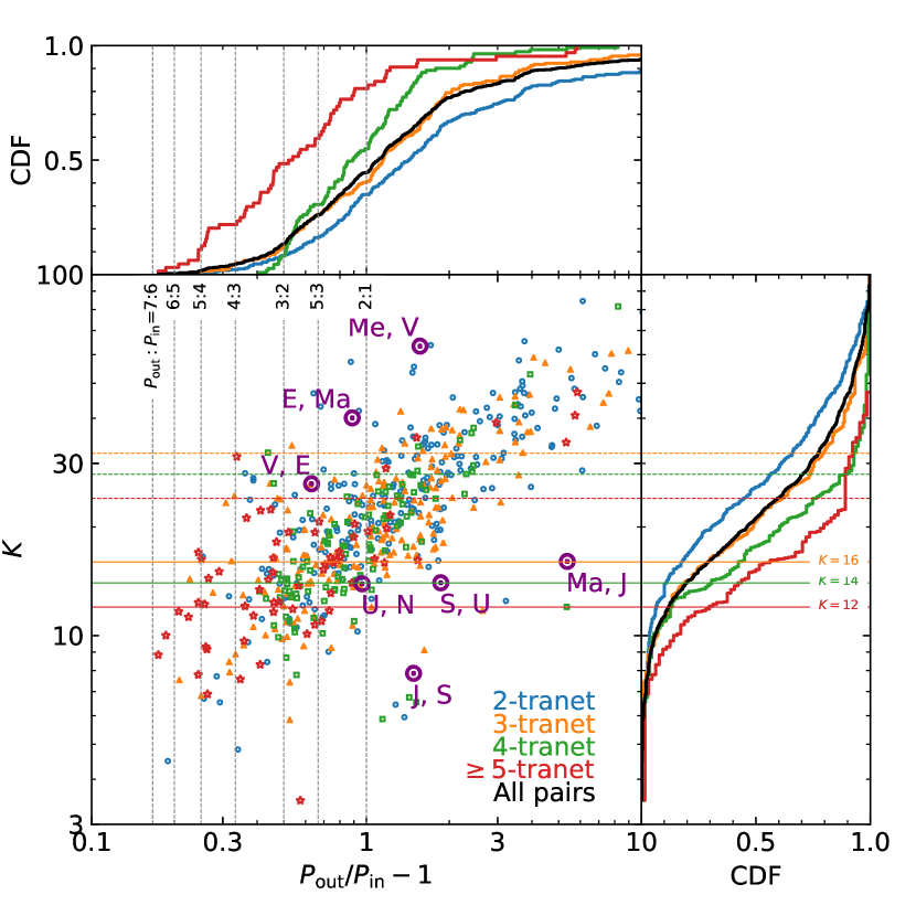
Figure 7: Spacings between the apparently adjacent planets in Kepler multi-planet systems, with different colors indicating planet pairs from different transit multiplicities. The $x$-axis of the main panel (lower left) shows the spacing in terms of the orbital period ratio, and the upper panel shows the corresponding cumulative distributions. A few example period commensurabilities are indicated in both panels. The $y$-axis of the main panel shows the spacing in terms of the mutual Hill radii (Equation 18), and the right panel shows the corresponding cumulative distributions. The stability thresholds for 3-tranet, 4-tranet, and 5-tranet systems, derived according to Equation 20, are indicated with solid horizontal lines. Values corresponding to twice of the thresholds are also shown as dashed horizontal lines. The code Forecaster from Chen & Kipping (2017) is used to predict the planet mass based on the planetary radius, and we have revised the upper mass limit to $10^{3}\,M_{\oplus}$ ($\sim 3~{}M_{\rm J}$) to avoid masses beyond the planetary regime. Solar system planet pairs are also indicated for references.

The relative positions of planets in Kepler multi-planet systems have also drawn lots of interest. The majority of the early studies focused on the period ratio distribution. As shown in Figure 7, Kepler systems contain very few planet pairs near/in low-order mean-motion resonances (see also Lissauer et al. 2011, Fabrycky et al. 2014). This is in contrast with earlier RV results that a substantial fraction of well-characterized multi-planet systems contain pairs of giant planets close to mean-motion resonances (e.g., Wright et al., 2011). We refer to Section 4.1 for the theoretical implications of this feature. Additionally, the asymmetry around exact period commensurabilities has also attracted lots of attention (Fabrycky et al., 2014), and we refer interested readers to the fairly comprehensive overview by Terquem & Papaloizou (2019) for this particular issue (see also the recent development by Millholland & Laughlin 2019). This review focuses on the dynamical compactness of the Kepler multi-planet systems, which concerns the long-term stability and thus the dynamical evolution.

When the stability of the planetary system is concerned, the orbital spacing between planets is usually expressed in the dimensionless parameter $K$

$$K\equiv\frac{a_{\rm out}-a_{\rm in}}{R_{\rm H}};\quad R_{\rm H}\equiv\frac{a_{\rm in}+a_{\rm out}}{2}\left(\frac{m_{\rm in}+m_{\rm out}}{3M_{\star}}\right)^{1/3}\ .$$ (18)

Here $R_{\rm H}$ is called the mutual Hill radius, $M_{\star}$ is the mass of the host star, and $a_{\rm in}$ ($a_{\rm out}$) and $m_{\rm in}$ ($m_{\rm out}$) are the semi-major axis and the mass of the inner (outer) planet, respectively. For two-planet systems, the condition for the long-term stability (and thus instability) has been well understood theoretically, and the instability arises when there are mean-motion resonance overlaps (Wisdom, 1980, Deck et al., 2013, Hadden & Lithwick, 2018). For systems with more than two planets, we lack a good theoretical understanding on the origin of the dynamical instability (see attempts by Chambers et al. 1996, Zhou et al. 2007, Quillen 2011, Yalinewich & Petrovich 2020). Nevertheless, numerical studies have shown that the timescale before which close encounter occurs between planets, $t$, scales exponentially with the initial spacing $K$ (Chambers et al., 1996). Details of this scaling relation depend on factors such as the number of planets, planet masses, orbital eccentricities and inclinations, as well as the inhomogeneity among planets (e.g., Chambers et al. 1996, Zhou et al. 2007, Funk et al. 2010; see Pu & Wu 2015 for a recent summary).

In the context of Kepler planetary systems, Pu & Wu (2015) found through numerical simulations that the median spacing for stability could be approximated as

$$\langle K\rangle=2.87+0.7\log_{10}{\tau}+2.4\left[\left(\frac{\sigma_{e}}{e_{\rm H}}\right)+\left(\frac{\sigma_{i}}{4e_{\rm H}}\right)\right],$$ (19)

where $\tau$ is the physical timescale $t$ scaled by the orbital period of the innermost planet, $e_{\rm H}$ is the mutual Hill radius scaled by the semi-major axis of the innermost planet, and $\sigma_{e}$ and $\sigma_{i}$ are the dispersions of orbital eccentricities and mutual inclinations among the planets, respectively. With the multiplicity-dependent $\sigma_{e}$ and $\sigma_{i}$ (Equation 14) and the typical values for Kepler systems ($t\gtrsim$ Gyr old and the innermost planet of planet-to-star mass ratio $q\approx 10^{-5}$ at $0.1~{}$AU), Equation 19 yields

$$\langle K\rangle\approx 10.2+2.2\left(\frac{k}{5}\right)^{\zeta}.$$ (20)

With $\zeta=-2$ (Zhu et al., 2018b, He et al., 2020), planetary systems with (3, 4, 5) Kepler planets should have critical spacings $\langle K\rangle=(16,~{}14,~{}12)$, respectively.

We apply the above stability thresholds to the multi-planet systems from Section 2.1 and discuss the limitations. After the use of Kepler’s third law, the only unknown to determine the spacing parameter $K$ is the planet-to-star mass ratio. We estimate the planetary masses from the measured radii with the Forecaster code from Chen & Kipping (2017) and adopt the Gaia stellar mass from Berger et al. (2020b). Systems without reported stellar mass measurements are excluded. Figure 7 illustrates the spacings between neighboring Kepler planets of all systems and systems divided into different transit multiplicities. For transit multiplicities of $3$, $4$, and $5+$, the majority ($\sim 70\%$) of planet pairs have spacings above the corresponding stability thresholds, confirming that they are indeed (most likely) long-term stable. The remaining $\sim 30\%$ planet pairs, considered long-term unstable by the above empirical thresholds, are probably stable as well. While part of this misclassification is due to the choice of fixed Kepler system parameters and the empirical (but sometimes unphysical) mass–radius relation (Chen & Kipping, 2017), it nevertheless is a sign for the failure of the empirically determined stability criteria. In particular, these stability criteria do not take into account the impact of mean-motion resonances, which can be either protective or destructive to the involved planets.

Nevertheless, by applying the empirical stability thresholds to the data one finds that the majority of Kepler planet pairs are not far from the empirical stability limits: The median spacing of all planet pairs is $K\approx 20$, and about $80$–$90\%$ of planet pairs from systems with at least three transiting planets have spacings within twice of the empirical stability thresholds (horizontal dashed lines in Figure 7). These results are consistent with previous findings (e.g., Fang & Margot, 2013, Pu & Wu, 2015, Weiss et al., 2018b) and also suggest that for the majority of Kepler planet pairs there is no room for inserting another (undetected) planet in between (Fang & Margot, 2013). In other words, the observed Kepler planets are dynamically packed. However, it does not necessarily mean that Kepler systems do not contain additional planets. The space to the innermost and particularly the outermost Kepler planet allows the existence of additional planets without risking instability. For example, seven planets with $q=10^{-5}$ are allowed per factor of 10 in semi-major axis if mutually separated by $K=20$. The observed dynamically packed structure is also probably due to the selection bias that it is increasingly difficult for both planets in a wider-spacing pair to transit the host star.

As part of the “peas in a pod” claim (see Section 2.4.1), the spacings between Kepler planets in the same multi-planet system are found to be statistically similar (Weiss et al., 2018b). However, the observed correlation in spacings is driven by a small fraction ($\lesssim 5\%$) of systems containing the highest multiplicities, and the majority of systems do not show such a regular spacing pattern (Zhu, 2020, Jiang et al., 2020).

2.5 Dependence of planet statistics on stellar properties

2.5.1 Impact of stellar companions

Stellar companions to the planet hosts affect the Kepler planet statistics in several ways. In transit surveys like Kepler, many of them appear unresolved and dilute the transit signals, potentially leading to misclassifications and erroneous planetary parameters (Ciardi et al., 2015, Bouma et al., 2018). Thankfully, follow-up high-resolution imaging observations have been performed for nearly all Kepler planet candidates (e.g., Furlan et al., 2017, Ziegler et al., 2018, and references therein). For bright targets that contain Jupiter-like transits, Santerne et al. (2016) also performed systematic radial-velocity follow-up observations and identified a significant false positive rate ($55\%$) for Jovian planet candidates. These efforts have led to a much better understanding of the impact of transit dilution on the Kepler planet statistics. In particular, Furlan et al. (2017) reported that about $10\%$ ($30\%$) of the candidate host stars have observed companions within $1^{\prime\prime}$ ($4^{\prime\prime}$), the majority of which are fairly faint compared to the target stars. In the most likely scenario that the transit signals come from the primary stars (see, e.g. Bouma et al., 2018), the dilution effect overall only affects the planetary radii up to a few percent on average (Furlan et al., 2017). This is within the uncertainty of Gaia-derived radii, and thus one does not expect it to have a significant impact on the general planet statistics. However, Earth-sized planets $R_{p}\lesssim 2\,R_{\oplus}$ are much more susceptible to the dilution effect, and thus the relevant statistics may suffer a more dramatic impact (Furlan et al., 2017, Bouma et al., 2018).

Besides the transit dilution effect, stellar companions can also affect the presence of planets through many dynamical processes (e.g., Artymowicz & Lubow, 1994, Holman & Wiegert, 1999). Very close ($a\lesssim 0.5~{}$AU) stellar binaries can host circumbinary (i.e., planetary-type or P-type) planets, and over a dozen such systems have been found (see Section 6.2 of Winn & Fabrycky 2015). We limit our discussions to the observational aspects of circumstellar (i.e., satellite-type or S-type) planets and the implications on planet statistics.

Studies based on RV and high-resolution imaging observations suggest that the existence of a close stellar-mass companion is usually associated with a lower frequency of circumstellar planets (e.g., Wang et al., 2014, 2015, Ngo et al., 2016, Kraus et al., 2016, Moe & Kratter, 2019). The effect of binary on the presence of close-in planets is quantified by a suppression factor $S_{\rm bin}$, which is the ratio between the fraction of planet hosts with stellar companions and the fraction of field stars with the same type of companions (Kraus et al., 2016, Moe & Kratter, 2019). Circumstellar planets are almost completely suppressed ($S_{\rm bin}\lesssim 15\%$) when the stellar companions are close (with separation $a_{\rm bin}\lesssim 10\,$AU), regardless of the planetary size or observed multiplicities. Planets are nearly unaffected ($S_{\rm bin}\gtrsim 85\%$) if the stellar companions are distant ($a_{\rm bin}\gtrsim 100\,$AU). At intermediate separations ($\sim 10$–$100\,$AU), the suppression effect gradually decreases with the increasing separation. See the Figure 3 of Moe & Kratter (2019) for a compilation of observational studies and an illustration of the suppression factor $S_{\rm bin}$ as a function of the binary separation.

With the above suppression effect and the known binary separation distribution, one can then infer the planet formation efficiency from the measured planetary system frequency $F_{\rm p}$. Moe & Kratter (2019) estimated that $F_{\rm bin}\approx 43\%$ of Sun-like primaries in a magnitude-limited survey like Kepler could not host close-in ($\lesssim 1~{}$AU) planets simply because of the influence of binary companions (see also Kraus et al., 2016). If these targets are excluded from the Kepler statistics, one finds that the formation efficiency of close-in planets around single stars, a parameter directly related to formation theories, should be $1/(1-F_{\rm bin})=1.8$ times higher than the fraction of stars with planets $F_{\rm p}$. This additional factor also provides a plausible explanation to the discrepancy in hot Jupiter frequencies measured from RV and Kepler (see Section 2.1.1).

2.5.2 Metallicity effect

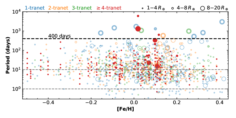
Figure 8: An illustration of the Kepler planetary systems in our baseline sample that have spectroscopic metallicity measurements. We use different colors to separate different observed multiplicities (out to 400 days) and different label sizes to separate planets of different sizes (small as 1–4$\,R_{\oplus}$, intermediate as 4–8$\,R_{\oplus}$, and giant as 8–20$\,R_{\oplus}$). Cold ($P>400\,$days) planets found by RV (as tabulated in Zhu & Wu 2018) and long-period transit searches (Kawahara & Masuda, 2019) are also indicated with thick circles. As the host metallicity increases, the system becomes more likely to contain giant planets at all periods and small planets at relatively close-in ($P\lesssim 10\,$days) orbits (e.g., Mulders et al., 2016, Dong et al., 2018, Petigura et al., 2018). At very high metallicities ([Fe/H]$\gtrsim 0.2$), there seems to be a deficit of compact systems (with $\geq 4$ transiting planets) and planets at intermediate orbits ($\sim$10–400 days). These may be related to the emerging cold giants (Zhu & Wu, 2018). The median metallicity of Kepler field stars is [Fe/H]$\approx 0.0$ (Dong et al., 2014b).

Under the general assumption that the bulk metallicity of the host star is correlated to the total mass of building blocks available for planet formation, it is reasonable to believe that the planetary occurrence rate and properties may be correlated with the host star metallicity. For giant planets ($R_{\rm p}\gtrsim 8\,R_{\oplus}$ or $m_{\rm p}\gtrsim 0.3\,M_{\rm J}$) found by RV, it has been well established that their presence correlates strongly with the host metallicity (e.g., Santos et al., 2001, Fischer & Valenti, 2005). This giant planet–metallicity correlation lends support to the core accretion model as the leading theory for the formation of giant planets (e.g., Pollack et al., 1996, Ida & Lin, 2004b). Some recent studies have also claimed that hosts of eccentric giant planets are more metal-rich than hosts of nearly circular giant planets (Dawson & Murray-Clay, 2013, Buchhave et al., 2018), but stronger statistical evidence is needed to fully establish this result.

Small planets, in particular those with radii $R_{\rm p}\lesssim 4\,R_{\oplus}$, show weaker dependences on host metallicity (e.g., Sousa et al., 2008, Buchhave et al., 2012). While many studies have focused on the dependence of the planet frequency $\bar{n}_{\rm p}$ on host metallicity (e.g., Wang & Fischer, 2015, Petigura et al., 2018) and theoretical implications (e.g., Owen & Murray-Clay, 2018, Lee, 2019), one may argue that the planetary system frequency $F_{\rm p}$ is probably a more suitable parameter to characterize the efficiency of planet formation under such system-wide parameters like metallicity (Zhu et al., 2016, Zhu, 2019). If the general planet–metallicity relation

$$F_{\rm p}\propto 10^{\gamma\rm[Fe/H]}$$ (21)

is applied, the result of Zhu (2019) suggests $\gamma\approx 0.5$ for all Kepler-type planets, which is much weaker than the giant planet–metallicity correlation ($\gamma\approx 2$; Fischer & Valenti 2005). The dependence is further reduced if the close binaries that show anti-correlation with stellar metallicity are excluded from the statistics (Moe et al., 2019, Kutra & Wu, 2020). Unlike the planetary system frequency $F_{\rm p}$, the planet frequency $\bar{n}_{\rm p}$ does not appear to have a monotonic relation with the host metallicity. In particular, it may start declining when the metallicity is high enough (Zhu, 2019). It has been suggested that this behavior may be related to the formation of giant planets inside the same system: as the metallicity is high enough, the system has a significant probability to form giant planets, and these giants may reduce the multiplicity of the inner system either because they prohibit the formation of more small planets or because they dynamically remove some of the small planets out of the inner system. This scenario may also explain the increased diversity of planets around metal-rich Kepler hosts (Petigura et al., 2018) and the over-abundant compact planetary systems around metal-poor stars (Zhu & Wu, 2018, Brewer et al., 2018). Figure 8 displays along the host metallicity [Fe/H] the Kepler systems with metallicity measurements in our baseline sample.

While the stellar bulk metallicity measured in iron abundance [Fe/H] (or a mix of metals [m/H]) is usually used in studies of the planet metallicity dependence, other elemental abundances, in particular $\alpha$ elements and refractory elements, have also been looked for possible correlations with planet properties (e.g., Adibekyan et al., 2012, Liu et al., 2016, Teske et al., 2019). No clear trends have been found so far, probably due to the limited sample size, the measurement precision, and/or the impact of Galactic chemical evolution.

2.5.3 Dependence on stellar mass

A number of studies have also investigated the dependence of planet frequency on host mass. A theoretical possibility is that, the stellar mass correlates with the total mass in the protoplanetary disk and thus the amount of solid materials available for planet formation. It is largely consistent with direct observations of protoplanetary disks in (sub-)millimeter wavelengths (Andrews et al., 2013, Ansdell et al., 2016), although at a fixed stellar mass the scatters of inferred disk masses remain substantial (up to an order of magnitude; Ansdell et al. 2016).

We would like to start by pointing out several potential issues. Similar to the metallicity dependence (see Section 2.5.2), the two frequencies, $F_{\rm p}$ and $\bar{n}_{\rm p}$, can behave differently, especially for the small planets with high multiplicity rates. Second, as more massive stars also tend to be more metal-rich, one may need to carefully disentangle possible correlation between stellar mass and metallicity in the sample (e.g., Johnson et al., 2010, Kutra & Wu, 2020). Furthermore, the choice of the parameter to study the correlation may matter. While planetary radius (or mass) and orbital period (or semi-major axis) are commonly used in statistical studies, Nature may prefer other physical units such as the planet-to-star mass ratio or the position of the water snow line (Hayashi 1981, Kennedy & Kenyon 2008; see Figure 10 for an illustration). Last but not least, as far as the planet formation efficiency is concerned, one must correct for the suppression effect due to close stellar binaries (see Section 2.5.1). It is established that the close binary fraction correlates with the primary mass (e.g., Duchêne & Kraus, 2013), so the suppression effect is expected to affect the statistics of planets around different stellar masses differently (Moe & Kratter, 2019).

The dependence of giant planets on stellar mass has been investigated in many studies with different detection methods (e.g., Johnson et al., 2007, 2010, Howard et al., 2012, Fressin et al., 2013, Nielsen et al., 2019). To avoid many of the issues listed above, here we focus on the results from long-term RV surveys, as they cover a broad range of parameter space and are nearly free of close stellar binaries. In particular, Johnson et al. (2010) analyzed a sample of 1266 stars with at least 3-year RV observations and masses spanning from $0.2\,M_{\odot}$ up to their estimated $1.9\,M_{\odot}$, and reported a linear relation between the occurrence rate and stellar mass. This result has been widely considered as a benchmark in both theoretical and observational studies of giant planets. The higher-mass part of the sample come from the so-called “retired A-stars,” and their spectroscopic mass estimates are controversial (Lloyd 2011, Schlaufman & Winn 2013, Malla et al. 2020 and references therein). Recently, the asteroseismic study by Malla et al. (2020) shows that the“retired A-stars” with spectroscopic masses $>1.6\,M_{\odot}$ are overestimated, confirming the earlier reports by Lloyd (2011) and Schlaufman & Winn (2013). Since such stars consist of the heavier half of the Johnson et al. (2010) sample and contribute most of the statistical evidence to the reported stellar mass dependence (see the Figure 4 of Johnson et al. 2010), a revisit of the mass correlation will be needed. Additionally, the result of Johnson et al. (2010) is limited to the region with separation $a<2.5\,$AU. As shown by Clanton & Gaudi (2014) and Clanton & Gaudi (2016), after those at (slightly) larger separations are taken into account, giant planets are almost as common around M-dwarfs as they are around Sun-like stars (see Section 3.3).

For small planets, Kepler survey provides the best sample to study their stellar mass dependence. Studies have shown that the planet frequency $\bar{n}_{\rm p}$ in the Kepler parameter space is anti-correlated with stellar mass (e.g., Howard et al., 2012, Mulders et al., 2015a, b). Using the Berger et al. (2018, 2020b) sample with stellar effective temperature between $4000$–$5000\,$K, we find a frequency of $\bar{n}_{\rm p}=3.3\pm 0.4$ for planets in the radius range $1$–$20\,R_{\oplus}$ and period $<400\,$days, which is a factor of $\sim 2.7$ higher than the rate for our baseline Sun-like sample (Section 2.1). Later M-type stars have even more planets (Dressing & Charbonneau, 2013, 2015). The planetary system frequency $F_{\rm p}$ is also anti-correlated with stellar mass but likely at a weaker level, due to the increased average planet multiplicity around later-type stars (e.g., Yang et al., 2020). There is some sign of increased observed multiplicity rate in our $4000$–$5000\,$K sample ($48.2\%$) compared to that ($42.5\%$) of our baseline Sun-like star sample (Section 2.1). After the correction for the suppression effect due to close stellar companions, the difference in formation efficiencies of small planets between single Sun-like and later-type hosts is likely further reduced, although an anti-correlation probably remains (Moe & Kratter, 2019).

3 THE OUTER PLANET POPULATION

In the earliest stage of planet formation, the region beyond $\sim 1\,$AU is expected to contain most of the mass and the angular momentum of the protoplanetary disk. Therefore, the frequency and properties of planets in this outer region ($\sim 1$–10 AU) have important implications to the formation and evolution of the whole system, including the planets in the inner $\sim 1\,$AU region. In this section, we review our current understanding of this outer planet population and discuss its connection with the inner planetary system.

We set the inner and outer boundary at $\sim 1\,$AU partly because this is approximately the detection limit of the Kepler mission, but also because it coincides with the position where giant planets show a rapid rise in frequency. RV surveys have found that giant planets ($m_{\rm p}\gtrsim M_{\rm Sat}\approx 0.3\,M_{\rm J}$) appear $\sim 5$ times more often between $\sim 1$–$3\,$AU than they do within $\sim 1\,$AU (Cumming et al., 2008).

3.1 Planet Frequency

RV surveys have found that cold giant planets (0.3–$13\,M_{\rm J}$) at $\sim$1–$5\,$AU) appear around on the order of $\sim 10\%$ of Sun-like stars. If the giant planet distribution is modeled as a parametric function that joins single power-law distributions of mass and orbital period (Tabachnik & Tremaine, 2002), the integrated rate out to $P\approx 5.5\,$years is found to be $\bar{n}_{\rm p}=0.105$ (Cumming et al., 2008). Such a single power-law period distribution tends to over-predict the number of giant planets at wider ($\gtrsim 10\,$AU) separations. To better match the observed distribution, Fernandes et al. (2019) replaced it with a broken power law and found a potential peak at $\sim$2–3 AU (see also Bryan et al. 2016). Extending their distribution function out to 100 AU, Fernandes et al. (2019) found $\bar{n}_{\rm p}=0.27_{-0.05}^{+0.08}$ and $0.062_{-0.012}^{+0.015}$ for planets in the mass range 0.1–20$\,M_{\rm J}$ and 1–20$\,M_{\rm J}$, respectively. If the frequency of the so-called Jupiter analogs, namely Jupiter-mass ($\sim$0.3–3$\,M_{\rm J}$) planets in Jupiter-like (a few AU) orbits around Sun-like hosts, are concerned, several independent studies have collectively pointed to a rate about a few percent (e.g., Wittenmyer et al. 2016 and references therein), suggesting that planetary systems similar to our own may be relatively uncommon (see also Section 3.2). Unlike our Jupiter, a significant fraction of cold giant exoplanets are on substantially eccentric orbits with typical eccentricities $e\sim 0.3$ (e.g., Wright et al., 2009). We refer to the review by Winn & Fabrycky (2015) for more discussions on these topics.

Although the region beyond $\sim 1\,$AU is nominally out of the reach of Kepler, studies have nevertheless systematically searched for and statistically studied the long-period transiting planets in the Kepler data (e.g., Foreman-Mackey et al., 2016, Herman et al., 2019, Kawahara & Masuda, 2019). In particular, Herman et al. (2019) reported an occurrence rate of $\bar{n}_{\rm p}=0.7_{-0.2}^{+0.4}$ for planets with sizes between 0.3–1$\,R_{\rm J}$ and orbital periods between 2–10 years. The inferred radius distribution also suggests that cold Neptune-sized (3–5 $M_{\oplus}$) planets are $\sim$4 times more common than cold Jupiter-sized (7.5–11 $M_{\oplus}$) ones. This is broadly consistent with the result from microlensing surveys (see Section 3.3), pointing to the potential existence of a large and unexplored low-mass planet population in the outer region.

3.2 The inner–outer correlation

The planetary systems inside and outside of $\sim 1\,$AU appear strongly correlated. Such a strong inner–outer correlation has important implications to the formation and evolution of the system as a whole. Below we review the observational evidence and discuss briefly the implications of this correlation. More on the latter will be presented in Section 4.2. We highlight two classes of inner planets, hot Jupiters and super Earths, and discuss them separately below.

3.2.1 “Friends” with close-in Jupiters

Hot Jupiters, while usually having no detectable planetary companions in the inner region, are frequently found to have distant massive companions (Knutson et al. 2014, Bryan et al. 2016; but see also Schlaufman & Winn 2016). Both of these features are important clues to the formation and evolution of hot Jupiters, and we refer interested readers to the review by Dawson & Johnson (2018) for in-depth discussions.

For the completeness of the discussion about the inner–outer correlation, we briefly summarize here the key result of the “friends of hot Jupiters” search. Knutson et al. (2014) conducted a systematic RV study of the distant companions to a sample of 51 hot Jupiters and reported that each hot Jupiter should have on average $0.51\pm 0.10$ companions with masses between 1–13$\,M_{\rm J}$ and semi-major axes between 1–20 AU. This sample was re-analyzed in Bryan et al. (2016) with improved sensitivity calculations, and the companion rate was revised to $0.70\pm 0.08$. Given the small fraction of systems with more than one cold companion, we take this average number to be approximately the fraction of hot Jupiter hosts with cold Jupiter companions. This fraction barely changes after we adjust to the parameter range used in this work (0.3–13$\,M_{\rm J}$ and 1–10 AU) according to the planet distribution function of Bryan et al. (2016). We denote this fraction as $P({\rm CJ}|{\rm HJ})$. Additionally, given the known fractions of Sun-like stars with hot Jupiters and cold Jupiters, $P({\rm HJ})\approx 1\%$ and $P({\rm CJ})\approx 10\%$, respectively, the inversed conditional probability is $P({\rm HJ}|{\rm CJ})\approx 7\%$. This is the fraction of cold Jupiter hosts with hot Jupiters. All the four fractions are shown in Figure 9.

Jupiter-sized planets in the inner region with known outer giant companions tend to have higher eccentricities, suggesting possible dynamical interactions in sculpting the architectures of these systems (e.g., Bryan et al., 2016). In particular, warm ($\sim 10$–$100\,$days) Jupiters on significantly eccentric orbits ($e\gtrsim 0.4$) have much higher chances to possess relatively close ($\lesssim 3\,$AU) Jovian companions compared to those on nearly circular ($e\lesssim 0.1$) orbits (Dong et al., 2014a), and the existence of such companions are consistent with the high-eccentricity migration scenario to form eccentric warm Jupiters (Dong et al., 2014a, Dawson & Chiang, 2014, Petrovich & Tremaine, 2016). By contrast, warm Jupiters on nearly circular orbits show a weaker correlation with outer giant companions, and many of these warm Jupiters are found to have nearby small planetary companions (Huang et al., 2016). These features cannot be easily reconciled in the high-eccentricity migration scenario, suggesting that the nearly circular warm Jupiters may have been formed in situ or have undergone the disk-driven migration (e.g., Raymond et al. 2008, Hallatt & Lee 2020). We refer to Dawson & Johnson (2018) for more comprehensive discussion on the observations and theories related to warm Jupiters.

3.2.2 Super Earth–cold Jupiter relation

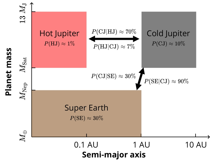
Figure 9: Correlations between inner planets and outer cold Jupiters. Although only two types of inner planets are highlighted here, they are representative of the known inner planet population: The majority of hot Jupiters do not have close neighbors (see Section 2.1.1), whereas super Earths usually reside in systems that include other types of inner planets (see Section 2.2). The unconditional probability shown here is the fraction of Sun-like stars with a specific type of planets, and the conditional probability is the fraction of Sun-like stars with a specific type of planets given that another type of planets is present in the system.

The term “super Earth” has different meanings in different studies. Here we call a planet super Earth if its mass (or radius) is between the masses (or radii) of Earth and Neptune, and the correlation under discussion applies specifically to the super Earths from the inner region. These super Earths dominate the known inner planet population, and they can co-exist with almost all types of inner planets except hot Jupiters (see Section 2.1). For this reason, this super Earth population is representative of the inner planet population.

About $1/3$ of the inner super Earths have outer cold Jupiter companions, as studies have shown (Zhu & Wu, 2018, Bryan et al., 2019). The RV signal on the star induced by a super Earth is systematically smaller than the RV signal induced by a cold Jupiter. Making use of this point, Zhu & Wu (2018) constructed a sample of 54 super Earth systems around Sun-like hosts that received long-term RV observations, and they found that the fraction of super Earth hosts with cold Jupiter companions is $32\pm 8\%$. This is $\sim 3$ times higher than the frequency of cold Jupiters around field Sun-like stars. The fraction further rises to $\sim 60\%$ for metal-rich systems (with [Fe/H]$>0.1$). These results were later confirmed by the independent study of Bryan et al. (2019). In that work the authors refit RV data sets of 65 super Earth hosts, some of which are M dwarfs, and reported an occurrence rate of $39\pm 7\%$ for companions with masses in the range 0.5–20$\,M_{\rm J}$ and semi-major axes in the range 1–20 AU. In this review, we take a rather conservative value of $P({\rm CJ}|{\rm SE})\approx 30\%$, which is also shown in Figure 9.

The inversion of the above conditional probability reveals an even more interesting result. With $\sim 30\%$ of Sun-like stars hosting inner super Earths and $\sim 10\%$ of Sun-like stars hosting cold Jupiters, one finds from the Bayes theorem that $P({\rm SE}|{\rm CJ})\approx 90\%$, suggesting that nearly all of the cold Jupiters should have inner small planets (Zhu & Wu, 2018, Bryan et al., 2019). Together with the fraction of cold Jupiter hosts with hot Jupiters, $P({\rm HJ}|{\rm CJ})\approx 7\%$, outer giant planets almost all have inner companions. We illustrate in Figure 9 the connections between the outer giant planets and the two representative types of inner planets.

The above strong correlations are also confirmed by studies that utilized the rare but valuable long-period Kepler transiting planets (Uehara et al., 2016, Herman et al., 2019, Masuda et al., 2020). These studies find that the fraction of long-period ($P\gtrsim 2\,$years) transiting planets with inner transiting companions is so high that it can only be explained by a strong inner–outer correlation. They also reported evidence that the dynamical hotness of inner and outer planets may also be correlated. Specifically, a dynamically hot outer Jupiter is likely associated with a dynamically hot inner planetary system. This provides a plausible explanation for the surprisingly large eccentricities and mutual inclinations of the inner systems with low multiplicities (Masuda et al. 2020; see Section 2.3). It may also help explain the reduced super Earth multiplicities around metal-rich stars (Zhu & Wu 2018; see Section 2.5.2).

The strong inner–outer correlation has implications on the frequency of planetary systems similar to our own. On the one hand, this correlation suggests that the general solar system-like architecture—with the inner region containing small planets and the outer region containing giant planets—is probably common among other planetary systems. On the other hand, planetary systems with properties very similar to ours, namely a system with both outer Jupiter-like ($\sim M_{\rm J}$ at a few AU) and inner Earth-like ($\lesssim M_{\oplus}$ within 1 AU) planets may be rare ($\lesssim 1\%$, Zhu & Wu 2018). A possible explanation could be that our Jupiter formed very early and hence prevented the growth of inner embryos into super Earths (Morbidelli et al., 2015, Izidoro et al., 2015). This early Jupiter formation scenario also explains the isotope measurements on solar system iron meteorites (Kruijer et al., 2017), although the question remains why the majority of cold Jupiters in other systems do have inner super Earths. We defer to Section 4.2 for further discussions of theoretical implications.

Observationally, the strong inner–outer correlation implies interesting synergies between space-based transit missions and astrometric missions or ground-based long-term RV surveys. Indeed, at least two of the TESS transiting planets have been found around stars with known RV cold Jupiters (Huang et al., 2018, Teske et al., 2020). Future combined TESS and Gaia planet catalogs should yield hundreds of similar systems that can enable detailed studies of the system architecture, as has been demonstrated in the pi Mensae system (Xuan & Wyatt, 2020, Damasso et al., 2020, De Rosa et al., 2020).

3.3 Mass-ratio function from microlensing

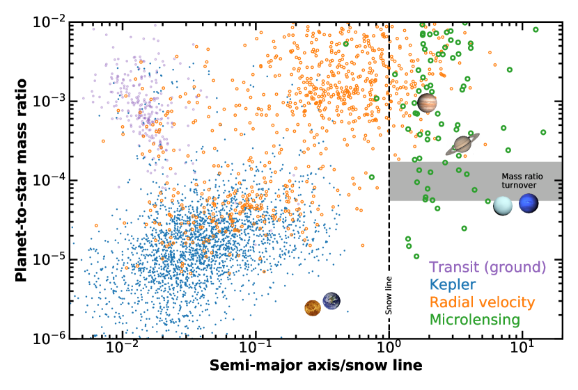
Figure 10: Similar to Figure 1, but here shows the planet-to-star mass ratio vs. the semi-major axis in units of the water snow line. The snow line is at $2.7\,$AU for $1\,M_{\odot}$ star and scales linearly with the host mass (Kennedy & Kenyon, 2008). The location of the snow line is indicated with a black dashed line (note that this is only for illustrative purposes as the snow line should be determined in the protoplanetary disk), and the possible turnover in the mass ratio distribution found from microlensing, $0.55$–$1.7\times 10^{-4}$ (Suzuki et al., 2016, Jung et al., 2019), is marked with the gray region. Six solar system planets are shown, with Mercury and Mars too low in mass ratio to appear on this plot.

Gravitational microlensing probes a largely uncharted planet discovery space of cold planets (Mao & Paczynski, 1991, Gould & Loeb, 1992), where $>99\%$ of the planetary mass of the solar system resides. Ground-based microlensing surveys are sensitive to planets down to Earth masses (e.g., Bennett & Rhie, 1996, Dong et al., 2006), and a space-based survey will be capable of discovering all solar system planet analogs except Mercury (Penny et al. 2019; see also Figure 1). With the increasing number of discoveries, microlensing searches have been continuing to unveil the distribution of planets in this under-explored parameter space and offer insights into the planet formation outside the water snow line. We refer interested readers to Gaudi (2012) for an overview of the microlensing technique and its application in exoplanet discoveries (see also Mao, 2012). Below we focus on the important progress made since the review of Gaudi (2012).

Several recent studies found evidence for a possible turnover in the planet-to-star mass ratio function for planets beyond the water snow line (see Figure 10). In the early era, a key microlensing finding was that cold Neptunes (with planet-to-star mass ratio $q\sim 10^{-4}$) are a factor of a few more common than cold Jupiters (with $q\sim 10^{-3}$, Gould et al. 2006b), and Sumi et al. (2010) found that the distribution of the mass ratio $q$ could be described by a power law ${dN}/d\log_{10}{q}\propto q^{\nu}$, where $\nu=-0.7\pm 0.2$. Using the planet sample from the MOA-II microlensing survey, Suzuki et al. (2016) found that a single power law of the mass ratio function does not extend to very low mass ratios. Specifically, these authors reported a break in the mass ratio function at $q\sim 10^{-4}$, corresponding to the mass of Neptune for a typical host star mass of $0.5\,M_{\odot}$. Based on a total sample of 30 planets that combines the MOA-II and previous statistical samples (Gould et al., 2010, Cassan et al., 2012), Suzuki et al. (2016) reported a broken power-law mass ratio function with a break at $q_{\rm brk}=1.7\times 10^{-4}$. The power-law indexes above and below the break are $\nu=-0.93\pm 0.13$ and $0.6^{+0.5}_{-0.4}$, respectively. The normalization is such that $\bar{n}_{\rm p}=0.79$ for planets with mass ratio $q>5\times 10^{-5}$ and projected separation $s$ in units of Einstein radius in the range 0.3–5. For typical microlenses with $0.5\,M_{\odot}$, these numbers correspond to the planetary mass $M_{\rm p}>8\,M_{\oplus}$ and the orbital separation between 1–15 AU. The reported planet frequency is compatible with those from other detection techniques (i.e., RV and direct imaging) following a simple joint planet distribution function (Clanton & Gaudi, 2014, 2016).

Further studies by Udalski et al. (2018), who studied an ensemble of seven (as compared to four in Suzuki et al. 2016) planets with $q<10^{-4}$, and Jung et al. (2019), who analyzed a sample of 15 planets with $q<3\times 10^{-4}$, investigated the possible turnover in the mass ratio function. Adopting a power-law form of the detection efficiency, Jung et al. (2019) modeled the intrinsic mass-ratio distribution with a broken power law and revised the break to $q_{\rm brk}\approx 5.5\times 10^{-5}$, which is a factor of three below the value found by Suzuki et al. (2016), but their low-mass planet sample was too small to distinguish a pile-up at that mass ratio from broken power law. Nevertheless, a break or pile-up in the planet-to-star mass ratio function could have important theoretical implications (e.g., Pascucci et al., 2018, Wu, 2019), and further probing the distribution of sub-Neptune microlensing planets will be a research focus in the near future. Observations from high-cadence and nearly continuous microlensing surveys such as KMTNet (Kim et al., 2016) are pushing toward detecting more planets at low mass ratios (e.g., $q=1.8\times 10^{-5}$ from Gould et al. 2020a, $q\approx 1.4\times 10^{-5}$ from Yee et al. 2021, $q\approx 1.1\times 10^{-5}$ from Zang et al. 2021), so a large enough sample is expected to be available soon to improve the determination of the mass ratio function at the low end (see Zang et al. 2021 and discussions therein).

Another interesting feature of the mass ratio function of Suzuki et al. (2016) is its apparent smoothness between Neptune and Jupiter masses. Intriguingly, the derived radius distribution of cold planets from the single transit events in Kepler also appears similarly continuous between Neptune and Saturn (Herman et al., 2019). These results are surprising in view of the standard core accretion theory (Pollack et al., 1996), which builds on the solar system and predicts a deficit of planets at such intermediate masses/radii (Ida & Lin, 2004a, Mordasini et al., 2009). This tension may suggest that the giant planet formation involves physical processes that have been overlooked in the standard models (Suzuki et al., 2018). Alternatively, it could be due to the limited sample sizes of cold intermediate-mass planets (Suzuki et al. 2016 sample contains nine detections in the range $10^{-4}<q<5\times 10^{-4}$ and Herman et al. 2019 has four in their intermediate radius bin of $0.67$–$1.00\,R_{\rm J}$). Therefore, increasing the sample size of cold intermediate-mass planets will clarify the degree of tension between observation and theory. Furthermore, physical mass (rather than mass ratio) determinations of a large sample of microlensing planets through measurements of the microlensing parallax or the lens flux (e.g., Dong et al., 2009) are needed to enable a more direct comparison with theories. This will be possible for essentially all microlensing planets detected to date at first light of adaptive optics on 30m class telescopes (e.g., Skidmore et al., 2015) or for a significant fraction of planet hosts in a space-based microlensing survey such as the Roman microlensing survey (Penny et al., 2019).

3.4 Free-floating planets

The prevalence of eccentric and/or inclined planetary orbits suggest likely histories of violent dynamical interactions in the planetary systems, such as planet-planet scatterings, which naturally eject a significant fraction of the planets from the system and form unbound planets with no hosts (e.g., Rasio & Ford, 1996b, Jurić & Tremaine, 2008, Chatterjee et al., 2008). The distributions of free-floating planets bear important signatures of not only the initial configurations of the planetary systems at birth, but also their subsequent dynamical evolution.

While it is possible to directly image young sub-stellar objects down to a few Jupiter masses (see, e.g., Zapatero Osorio et al., 2000), gravitational microlensing is the only known method in probing the lower-mass objects, which are believed to dominate the dynamically ejected FFP population. Low-mass objects produce relatively short-timescale microlensing light curves as the Einstein radius crossing time $t_{\rm E}\propto\sqrt{M}$. For typical stellar-mass microlenses, the timescale is $\sim 20\,$days, whereas for planetary-mass objects it is $\lesssim 1\,$day. The detection of such short and rare events thus demands wide-field high-cadence surveys that have only been available since the past decade.

Mróz et al. (2017) analysed a sample of 2,617 microlensing events from the OGLE-IV survey and concluded that the frequency of Jupiter-mass free-floating (or wide-orbit) planets should be no more than $0.25$ planets per main-sequence star at the 95% confidence level. This result is broadly compatible with the inferred occurrence rate of bound giant planets from RV surveys (e.g., Cumming et al., 2008), microlensing searches (e.g., Gould et al., 2010) or direct imaging (e.g., Bowler, 2016), and contradicts a previous claim that free-floating Jupiter-mass planets are more abundant than stars (Sumi et al., 2011). The sample of Mróz et al. (2017) also includes six short events with timescales in the range $0.1\,{\rm days}<t_{\rm E}<0.4\,{\rm days}$. Assuming the microlensing nature of these events and given the low detection efficiency at such ultrashort timescales, their sample suggests that there may be up to a few free-floating planets in the Earth-mass to super-Earth-mass range per main-sequence star. The results of Mróz et al. (2017) about the absence of free-floating Jupiter-mass planets and the potential existence of free-floating Earth-mass and super-Earth-mass planets are generally consistent with theoretical expectations (e.g., Ida et al., 2013, Ma et al., 2016).

The existence of such ultrashort-timescale events was soon confirmed thanks to the coordinated observations of multiple microlensing survey telescopes around the globe. Mróz et al. (2018) reported the first convincing example of a microlensing event with timescale $t_{\rm E}=0.32\,$days, and subsequent dedicated searches led to the discovery of a few more similar events (Mróz et al., 2019, 2020b, 2020a, Kim et al., 2020, Ryu et al., 2020). These events all show strong finite-source effects that arise from the lenses transiting distant giant sources, yielding the immediate measurement of the angular Einstein radius $\theta_{\rm E}$. The lens mass scales as

$$M({\rm bulge})=\frac{\theta_{\rm E}^{2}}{\kappa\pi_{\rm rel}}=250\,M_{\oplus}\left(\frac{\theta_{\rm E}}{10\,\mu{\rm as}}\right)^{2}\left(\frac{\pi_{\rm rel}}{16\,\mu{\rm as}}\right)^{-1},$$ (22)

with the normalization of the lens-source relative parallax $\pi_{\rm rel}$ chosen such that the lens and source are both in the Galactic bulge and separated by about $1\,{\rm kpc}$. Here the constant $\kappa\approx 8.14\,{\rm mas}\,M_{\odot}^{-1}$. For lens in the Galactic disk ($\pi_{\rm rel}\approx 125\,\mu{\rm as}$), the mass scales as

$$M({\rm disk})=\frac{\theta_{\rm E}^{2}}{\kappa\pi_{\rm rel}}=32\,M_{\oplus}\left(\frac{\theta_{\rm E}}{10\,\mu{\rm as}}\right)^{2}\left(\frac{\pi_{\rm rel}}{125\,\mu{\rm as}}\right)^{-1}.$$ (23)

Kim et al. (2020) and Ryu et al. (2020) argue that $\theta_{\rm E}$ is a better discriminator than $t_{\rm E}$ for selecting FFPs. In fact, from a small number of events with finite-source effects, there is a possible gap between $\sim 10\,\mu{\rm as}$ and $\sim 30\,\mu{\rm as}$ in the $\theta_{\rm E}$ distribution, and this “Einstein desert” may separate brown dwarfs from free-floating super Earths (and terrestrial planets) in the disk (Ryu et al., 2020). We list in Table 1 the relevant parameters and inferred masses of the FFP candidate events with $\theta_{\rm E}<10\,\mu{\rm as}$. The preliminary analyses by Mróz et al. (2019) and Ryu et al. (2020) suggest that low-mass unbound (or wide-orbit) planets may be more common than stars in the Galaxy. Future space-based microlensing surveys can assemble a large sample for quantitative assessments of the FFP population (e.g., Johnson et al., 2020), and a satellite augmented with microlensing parallax measurements can directly measure the masses and distances of such FFP events (e.g., Gould et al., 2020b, and references therein).

Table 1: Published microlensing free-floating planet candidates ($\theta_{\rm E}<10\mu{\rm as}$), sorted by the inferred lens mass (see Equation 22 and Equation 23 for typical estimates in the bulge and disk, respectively).

Event name	$\theta_{\rm E}/\mu{\rm as}$	$t_{\rm E}/{\rm d}$	$M({\rm disk})$	$M({\rm bulge})$	Reference
OGLE-2016-BLG-1928	0.84	0.029	$0.2\,M_{\oplus}$	$1.8\,M_{\oplus}$	Mróz et al. (2020a)
OGLE-2012-BLG-1323	2.4	0.16	$1.8\,M_{\oplus}$	$14\,M_{\oplus}$	Mróz et al. (2019)
OGLE-2019-BLG-0551	4.4	0.38	$6.1\,M_{\oplus}$	$48\,M_{\oplus}$	Mróz et al. (2020b)
KMT-2019-BLG-2073	4.8	0.27	$7.6\,M_{\oplus}$	$59\,M_{\oplus}$	Kim et al. (2020)
KMT-2017-BLG-2820	5.9	0.29	$11\,M_{\oplus}$	$87\,M_{\oplus}$	Ryu et al. (2020)
OGLE-2016-BLG-1540	9.2	0.32	$28\,M_{\oplus}$	$217\,M_{\oplus}$	Mróz et al. (2018)

While the events listed in Table 1 are promising candidates for FFPs, it is also plausible that these objects are actually in such wide orbits that no microlensing signatures from their hosts were detected. Light curve analyses can exclude the existence of any massive companions (i.e., hosts) out to a few Einstein radii, corresponding to $\sim 15$–$20\,$AU away (e.g., Mróz et al., 2018, Kim et al., 2020). In other words, these FFP candidates could well be planets at Uranus-like or Neptune-like orbits (e.g., Poleski et al., 2014). Future high-resolution imaging observations that can resolve the hosts for wide-separation planets will be able to tell whether these objects are truly free-floating or loosely bound to some unidentified stellar hosts (Han et al., 2005, Gould, 2016, Ryu et al., 2020).

4 THEORETICAL IMPLICATIONS

The observed distribution of planets and the architecture of planetary systems, as reviewed in Sections 2 and 3, are the consequence of $\sim$10–100 Myr formation and later $\sim$Gyr evolution. In this section, we discuss the constraints from these observations on theoretical models. A comprehensive overview on the formation and evolution theories is beyond the scope of the current review. Instead, we focus on the key physical processes that lead to observational signatures. To reduce the complexity, we restrict to planetary systems around Sun-like hosts.

4.1 A brief overview of theories

The generally accepted picture of planet formation can be traced back to the nebular model originally proposed by Immanuel Kant and Pierre Laplace in the 1700s. Modern theorists generally believe that planets were formed out of the gas and the dust in the protoplanetary disk. Small solid particles first accumulate to form asteroid-sized ($\sim$1–100 km) planetesimals, and the collisions between planetesimals eventually lead to the formation of planet-sized objects (Chamberlin, 1916, Safronov, 1972). See Woolfson (1993) for a historical overview on the planet formation theories.

In the core accretion theory that explains the solar system formation(e.g., Lissauer, 1993, Pollack et al., 1996), the primary building blocks for planet formation are planetesimals. The growth of planetesimals is first divergent (i.e., the run-away phase) and then convergent (i.e., the oligarchic phase), until they have cleared nearly all planetesimals in their feeding zone ($\sim 5\,R_{\rm H}$). These so-called protoplanets (or embryos) are now $\gtrsim 1000\,$km in size and around Mars-mass (e.g., Ida & Makino, 1993, Kokubo & Ida, 1998). The further growth of the protoplanets involves planetesimal accretion as well as dynamical interactions between protoplanets. At a few AU separation, the growth of protoplanets is sufficient and allows the formation of giant planets (Mizuno, 1980, Pollack et al., 1996). In the classical picture, the giant planet formation has three phases: core formation, hydrostatic gas accretion, and run-away gas accretion (Pollack et al., 1996). The hydrostatic gas accretion phase starts when the embryo reaches a critical core mass ($\sim 10\,M_{\oplus}$, Mizuno 1980, Stevenson 1982). This phase can take up to $\sim 10\,$Myr and is the most time-consuming step in this classical core accretion model. The run-away gas accretion is triggered once the envelope and the core have comparable masses, and it sufficiently pushes the total mass to the giant planet regime ($\gtrsim 100\,M_{\oplus}$). In the inner region, embryos grow slowly and never reach the critical core mass before the gaseous disk is depleted. The later evolution involves collisions between these embryos in the gas-free environment. This so-called giant impact phase lasts $\sim 100\,$Myr and eventually forms the terrestrial planets (e.g., Chambers, 2001).

A new paradigm that has attracted much attention recent years is pebble accretion. In the astrophysical context, pebbles are dust particles that are weakly coupled to the gas and thus drift in the disk. The inclusion of pebbles in the formation diagram provides a plausible scenario for the formation of planetesimals via streaming instability (Youdin & Goodman, 2005, Johansen et al., 2007, Chiang & Youdin, 2010). Unlike planetesimals that are decoupled from the gas, pebbles “feel” the aerodynamic drag from the gas and drift inward toward the star (Nakagawa et al., 1986). This means that the “food” supply to a protoplanet is not limited to the local material. Additionally, the cross-section for protoplanets (or planetesimals) to accrete pebbles is larger than the cross-section for the same objects to accrete planetesimals (Ormel & Klahr, 2010, Lambrechts & Johansen, 2012). These two factors together make pebble accretion more efficient in building up cores of protoplanets. When the protoplanet becomes massive enough, it starts to carve a gap in the pebble disk, and the subsequent pressure bump outside of the orbit stops the inward drifting pebbles. The corresponding mass of the protoplanet is called the pebble isolation mass

$$M_{\rm iso}\approx 10\left(\frac{h/r}{0.04}\right)^{3}\,M_{\oplus}~{},$$ (24)

where $h/r$ is the disk aspect ratio at location $r$ and the prefactor is determined numerically and depends on disk properties (Lambrechts et al., 2014). The above relation assumes a solar-mass host star. For other stellar masses, the pebble isolation mass scales linearly with the mass of the host star (Liu et al., 2019). Once a protoplanet reaches the pebble isolation mass, it effectively cuts off the pebble flux and “starves” the protoplanetary core and all embryos interior to its orbit. With the halted pebble accretion, the critical core mass required to trigger the rapid gas accretion is reduced and thus giant planets can form more efficiently (Lambrechts et al., 2014). Furthermore, pebbles can easily vaporize in the hot envelopes before they can reach the cores (Brouwers et al., 2018). The enriched envelopes also speed up the formation of giant planets (Venturini et al. 2016; see also Stevenson 1982 and Hori & Ikoma 2011 for a similar mechanism in the planetesimal accretion scenario). We refer interested readers to the reviews by Johansen & Lambrechts (2017) and Ormel (2017) for more details about the pebble accretion model.

Planets may undergo disk-driven migration while accreting pebbles, planetesimals, and/or gas (e.g., Kley & Nelson 2012 and references therein). Migration can substantially change the architecture of the planetary system, such as locking planets into mean motion resonances (Goldreich & Tremaine, 1980, Lee & Peale, 2002). However, such features are not prominent in Kepler systems (see Section 2.4.2). This may suggest that most Kepler planets have not undergone significant disk-driven migrations (see also Section 4.2). Alternatively, the Kepler planets may have never entered into resonances during the migration (e.g., Goldreich & Schlichting, 2014), or the long-term dynamical evolution after the disk dispersal has effectively removed most of these features (e.g., Izidoro et al., 2017, 2019).

4.2 Constraints from observations

Given the substantial uncertainties in theories and in some parts of observations, we think that it is premature to provide detailed and quantitative comparisons between theories and observations (but see attempts by, e.g., Hansen & Murray 2013, Izidoro et al. 2017, Mulders et al. 2019, Emsenhuber et al. 2020). We therefore choose to focus on some selected constraints that are considered relatively robust and discuss their implications to the formation of Kepler-like planets:

• Prevalence and multiplicity. Inner super Earth-like planets are known to exist around $\sim 30\%$ Sun-like stars, and they typically reside in multi-planet systems (Section 2.2). Additionally, they preferentially have outer cold Jupiter companions (Section 3.2), suggesting that the two types of planets do not inhibit, but perhaps promote, the formation of each other. Unlike giant planets, super Earths show a much weaker dependence on the host metallicity (Section 2.5.2).

• Composition. As inferred from population-level studies of the radius valley (Section 2.1.4) as well as mass and radii measurements of individual Kepler planets (e.g., Wu & Lithwick, 2013, Hadden & Lithwick, 2014, 2017), some inner small planets likely have Earth-like (i.e., rocky and ice-poor) cores, and these cores have acquired gaseous envelopes that weigh up to a few percent of the total mass while the disk is still present.

The prevalence and the early formation of super Earth-like planets suggest that the planet formation process is more efficient than what had been expected from solar system formation models (e.g., Ida & Lin, 2004a, Mordasini et al., 2009). This alone may not be an issue to the pebble accretion scenario (see Section 4.1). In fact, pebble accretion can be so efficient that preventing super Earth-mass planets from undergoing run-away gas accretion places another challenge, a possible solution to which could be a delayed formation near the end of the disk phase (e.g., Lee et al., 2014). For the planetesimal accretion scenario, a very massive disk is typically required to form super Earths efficiently and early (e.g., Emsenhuber et al., 2020). The rocky composition suggests that the cores are formed in the ice-poor environment, likely inside the water ice line. In order for embryos or protoplanets from outside of the ice line to not largely contaminate the inner region, the disk-driven migration is probably suppressed.

The strong correlation between inner super Earths and outer cold Jupiters is a bit challenging to both accretion scenarios under the typical protoplanetary disk conditions. The planetesimal accretion scenario usually requires relatively efficient disk-driven migrations to explain the presence of abundant super Earths around metal-poor hosts, but the same migration efficiency turns out an overkill in reproducing the inner–outer strong correlation (Schlecker et al. 2020, see also Ida & Lin 2010). For the pebble accretion scenario, because the solid supply to protoplanets is not limited locally, there is potentially a direct competition between different embryos. Furthermore, once the core of the outer giant planet first reaches the pebble isolation mass, the further growth of the inner planets is significantly limited, and the giant planet also acts as a barrier to the inward migrating embryos from outside of its orbit. Therefore, the pebble accretion scenario typically expects an anti-correlation between inner and outer planets (Morbidelli et al., 2015, Izidoro et al., 2015, Lambrechts et al., 2019). Alternatively, the cores of both inner super Earths and outer cold Jupiters could be formed at such large separations (tens of AU) that enough material is available to the inner cores (Bitsch et al., 2015, 2019), although it is unclear whether such an approach can reproduce quantitatively the observed correlation and forms rocky core planets. The difficulty in reproducing the inner–outer correlation may suggest that many protoplanetary disks start heavier than what has been typically assumed. Indeed, if Kepler planets are formed in situ based on the local material (i.e., not the inward-drifting pebbles), the required surface density is much higher than the minimum-mass solar nebula model (Weidenschilling, 1977, Hayashi, 1981) and almost reaches the gravitational instability limit (Chiang & Laughlin, 2013, Schlichting, 2014).

5 SUMMARY AND DISCUSSION

The discovery of thousands of exoplanets from the combination of multiple detection techniques have substantially advanced our understanding of the distribution of planets and the architecture of planetary systems. This review aims to update our knowledge of exoplanet statistics since the Winn & Fabrycky (2015) review. In Section 2, we described the distribution and properties of planets in the inner region, based mostly on discoveries from the Kepler mission. In Section 3, we reviewed the recent progress on the cold planet population, with an emphasis on their connections to the close-in companions. Section 4 briefly described the theoretical models and the key constraints from observations. We summarize the key results below:

[SUMMARY POINTS]

1. In the inner region ($\lesssim 1\,$AU), about $30\%$ of Sun-like stars host planets with masses/radii down to Earth mass/radii, and each planetary system on average has about three such planets. These suggest that the planet formation process is more efficient than what had been expected from solar system formation models.

2. Planetary systems with more planets appear colder dynamically, with smaller orbital eccentricities, mutual inclinations, and orbital spacings. For systems with few planets in the inner region, planets can have $\sim 0.3$ orbital eccentricities and $\gtrsim 10^{\circ}$ mutual inclinations. These support the idea that dynamical evolution has played a significant role reshaping the system architecture.

3. There exists a “radius valley” at $R_{\rm p}\sim 2\,R_{\oplus}$ and $P\lesssim 30\,$days. The valley was predicted by the photoevaporation theory, although alternative explanations have also been proposed. Population-level analyses of the radius valley suggest that these planets were probably born with rocky cores and gaseous atmospheres up to a few percent of the core masses.

4. Cold Neptune-like planets are a few times more abundant than cold Jupiter-like ones in the outer region. The inner ($\lesssim 1\,$AU) and the outer ($\sim$1–10 AU) planetary systems appear strongly correlated such that inner small planets preferentially have cold Jupiter-like companions and that outer cold Jupiters almost always have inner planetary companions.

With the ongoing and upcoming missions that have better capabilities and/or open up new observational channels, our understanding of exoplanets and planetary systems will continue to be improved. We outline below several promising directions that may see substantial advancement in the near future: [FUTURE PROSPECTS]

1. Exoplanet atmosphere and mass–radius relation: Space-based all-sky transit surveys like the TESS mission (Ricker et al., 2015) have been finding many bright targets, enabling detailed characterizations of more close-in planets (e.g., Huang et al., 2018, Armstrong et al., 2020). An improved mass–radius relation and better atmospheric characterizations will help to understand the composition and potentially the past evolution of the planet (see the recent review by Madhusudhan 2019)

2. Planetary system architecture: The joint coverage of different surveys will potentially open up a larger parameter space (see Figure 1) and reveal more interesting features about the planetary system architecture. The Gaia mission alone is expected to detect at least thousands of giant planets around nearby stars (Perryman et al., 2014), and its synergy with other surveys/missions will also open up new channels into the architecture study (e.g., Xuan & Wyatt, 2020, Damasso et al., 2020, De Rosa et al., 2020). RV follow-ups of systems detected by other methods could also play increasingly indispensable roles in this aspect, in particular with the extreme RV instruments with capability down to $\sim 0.3\,{\rm m\,s^{-1}}$ now coming online (e.g., Fischer et al., 2016).

3. Planet across the HR diagram: Rapid advances of large-scale spectroscopic surveys and the Gaia satellite are continuing to revolutionize stellar astrophysics and Galactic astronomy. Further synergies of large samples of exoplanets with detailed stellar chemical compositions, kinematics and/or ages measurements are expected to place planet formation in the rich context of stellar populations and evolutions.

4. Planets around young stars: While the present review focused on the planetary systems around $\gtrsim$Gyr old stars, the demographics of planets around young ($\lesssim 100\,$Myr) stars is a crucial link toward a more direct comparison with both planet formation theories and ALMA observations of protoplanetary disks (see the recent review by Andrews 2020). The detection and characterization of more planets around young stars (e.g., PDS 70b, c, Haffert et al. 2019 and AU Microscopii b, Plavchan et al. 2020) will be valuable.

DISCLOSURE STATEMENT

The authors are not aware of any affiliations, memberships, funding, or financial holdings that might be perceived as affecting the objectivity of this review.

References

- Adibekyan et al. (2012) Adibekyan VZ, Sousa SG, Santos NC, Delgado Mena E, González Hernández JI, et al. 2012. A&A 545:A32
- Agol et al. (2005) Agol E, Steffen J, Sari R, Clarkson W. 2005. MNRAS 359:567–579
- Akeson et al. (2013) Akeson RL, Chen X, Ciardi D, Crane M, Good J, et al. 2013. PASP 125:989
- Andrews (2020) Andrews SM. 2020. ARA&A 58:483–528
- Andrews et al. (2013) Andrews SM, Rosenfeld KA, Kraus AL, Wilner DJ. 2013. ApJ 771:129
- Ansdell et al. (2016) Ansdell M, Williams JP, van der Marel N, Carpenter JM, Guidi G, et al. 2016. ApJ 828:46
- Armstrong et al. (2020) Armstrong DJ, Lopez TA, Adibekyan V, Booth RA, Bryant EM, et al. 2020. Nature 583:39–42
- Artymowicz & Lubow (1994) Artymowicz P, Lubow SH. 1994. ApJ 421:651
- Bailey & Batygin (2018) Bailey E, Batygin K. 2018. ApJ 866:L2
- Ballard & Johnson (2016) Ballard S, Johnson JA. 2016. ApJ 816:66
- Beaugé & Nesvorný (2013) Beaugé C, Nesvorný D. 2013. ApJ 763:12
- Becker et al. (2015) Becker JC, Vanderburg A, Adams FC, Rappaport SA, Schwengeler HM. 2015. ApJ 812:L18
- Bennett & Rhie (1996) Bennett DP, Rhie SH. 1996. ApJ 472:660
- Berger et al. (2018) Berger TA, Huber D, Gaidos E, van Saders JL. 2018. ApJ 866:99
- Berger et al. (2020a) Berger TA, Huber D, Gaidos E, van Saders JL, Weiss LM. 2020a. AJ 160:108
- Berger et al. (2020b) Berger TA, Huber D, van Saders JL, Gaidos E, Tayar J, Kraus AL. 2020b. AJ 159:280
- Bitsch et al. (2019) Bitsch B, Izidoro A, Johansen A, Raymond SN, Morbidelli A, et al. 2019. A&A 623:A88
- Bitsch et al. (2015) Bitsch B, Lambrechts M, Johansen A. 2015. A&A 582:A112
- Borucki et al. (2010) Borucki WJ, Koch D, Basri G, Batalha N, Brown T, et al. 2010. Science 327:977
- Bouma et al. (2018) Bouma LG, Masuda K, Winn JN. 2018. AJ 155:244
- Bowler (2016) Bowler BP. 2016. PASP 128:102001
- Brewer et al. (2018) Brewer JM, Wang S, Fischer DA, Foreman-Mackey D. 2018. ApJ 867:L3
- Brouwers et al. (2018) Brouwers MG, Vazan A, Ormel CW. 2018. A&A 611:A65
- Bryan et al. (2016) Bryan ML, Knutson HA, Howard AW, Ngo H, Batygin K, et al. 2016. ApJ 821:89
- Bryan et al. (2019) Bryan ML, Knutson HA, Lee EJ, Fulton BJ, Batygin K, et al. 2019. AJ 157:52
- Buchhave et al. (2018) Buchhave LA, Bitsch B, Johansen A, Latham DW, Bizzarro M, et al. 2018. ApJ 856:37
- Buchhave et al. (2012) Buchhave LA, Latham DW, Johansen A, Bizzarro M, Torres G, et al. 2012. Nature 486:375–377
- Burke & Catanzarite (2017a) Burke CJ, Catanzarite J. 2017a. Planet Detection Metrics: Per-Target Detection Contours for Data Release 25. Kepler Science Document KSCI-19111-002
- Burke & Catanzarite (2017b) Burke CJ, Catanzarite J. 2017b. Planet Detection Metrics: Per-Target Flux-Level Transit Injection Tests of TPS for Data Release 25. Kepler Science Document KSCI-19109-002
- Burke et al. (2015) Burke CJ, Christiansen JL, Mullally F, Seader S, Huber D, et al. 2015. ApJ 809:8
- Burt et al. (2020) Burt JA, Nielsen LD, Quinn SN, Mamajek EE, Matthews EC, et al. 2020. AJ 160:153
- Cañas et al. (2019) Cañas CI, Wang S, Mahadevan S, Bender CF, De Lee N, et al. 2019. ApJ 870:L17
- Cassan et al. (2012) Cassan A, Kubas D, Beaulieu JP, Dominik M, Horne K, et al. 2012. Nature 481:167–169
- Chamberlin (1916) Chamberlin TC. 1916. JRASC 10:473
- Chambers (2001) Chambers JE. 2001. Icarus 152:205–224
- Chambers et al. (1996) Chambers JE, Wetherill GW, Boss AP. 1996. Icarus 119:261–268
- Chaplin & Miglio (2013) Chaplin WJ, Miglio A. 2013. ARA&A 51:353–392
- Chatterjee et al. (2008) Chatterjee S, Ford EB, Matsumura S, Rasio FA. 2008. ApJ 686:580–602
- Chen & Kipping (2017) Chen J, Kipping D. 2017. ApJ 834:17
- Chiang & Laughlin (2013) Chiang E, Laughlin G. 2013. MNRAS 431:3444–3455
- Chiang & Youdin (2010) Chiang E, Youdin AN. 2010. Annual Review of Earth and Planetary Sciences 38:493–522
- Christiansen et al. (2020) Christiansen JL, Clarke BD, Burke CJ, Jenkins JM, Bryson ST, et al. 2020. AJ 160:159
- Christiansen et al. (2015) Christiansen JL, Clarke BD, Burke CJ, Seader S, Jenkins JM, et al. 2015. ApJ 810:95
- Ciardi et al. (2015) Ciardi DR, Beichman CA, Horch EP, Howell SB. 2015. ApJ 805:16
- Ciardi et al. (2013) Ciardi DR, Fabrycky DC, Ford EB, Gautier T. N. I, Howell SB, et al. 2013. ApJ 763:41
- Clanton & Gaudi (2014) Clanton C, Gaudi BS. 2014. ApJ 791:91
- Clanton & Gaudi (2016) Clanton C, Gaudi BS. 2016. ApJ 819:125
- Cumming et al. (2008) Cumming A, Butler RP, Marcy GW, Vogt SS, Wright JT, Fischer DA. 2008. PASP 120:531
- Dai et al. (2018) Dai F, Masuda K, Winn JN. 2018. ApJ 864:L38
- Damasso et al. (2020) Damasso M, Sozzetti A, Lovis C, Barros SCC, Sousa SG, et al. 2020. A&A 642:A31
- Dawson & Chiang (2014) Dawson RI, Chiang E. 2014. Science 346:212–216
- Dawson & Johnson (2018) Dawson RI, Johnson JA. 2018. ARA&A 56:175–221
- Dawson & Murray-Clay (2013) Dawson RI, Murray-Clay RA. 2013. ApJ 767:L24
- De Cat et al. (2015) De Cat P, Fu JN, Ren AB, Yang XH, Shi JR, et al. 2015. ApJS 220:19
- De Rosa et al. (2020) De Rosa RJ, Dawson R, Nielsen EL. 2020. A&A 640:A73
- Deck et al. (2013) Deck KM, Payne M, Holman MJ. 2013. ApJ 774:129
- Dong et al. (2006) Dong S, DePoy DL, Gaudi BS, Gould A, Han C, et al. 2006. ApJ 642:842–860
- Dong et al. (2009) Dong S, Gould A, Udalski A, Anderson J, Christie GW, et al. 2009. ApJ 695:970–987
- Dong et al. (2014a) Dong S, Katz B, Socrates A. 2014a. ApJ 781:L5
- Dong et al. (2018) Dong S, Xie JW, Zhou JL, Zheng Z, Luo A. 2018. Proceedings of the National Academy of Science 115:266–271
- Dong et al. (2014b) Dong S, Zheng Z, Zhu Z, De Cat P, Fu JN, et al. 2014b. ApJ 789:L3
- Dong & Zhu (2013) Dong S, Zhu Z. 2013. ApJ 778:53
- Dressing & Charbonneau (2013) Dressing CD, Charbonneau D. 2013. ApJ 767:95
- Dressing & Charbonneau (2015) Dressing CD, Charbonneau D. 2015. ApJ 807:45
- Duchêne & Kraus (2013) Duchêne G, Kraus A. 2013. ARA&A 51:269–310
- Emsenhuber et al. (2020) Emsenhuber A, Mordasini C, Burn R, Alibert Y, Benz W, Asphaug E. 2020. arXiv e-prints :arXiv:2007.05562
- Fabrycky et al. (2014) Fabrycky DC, Lissauer JJ, Ragozzine D, Rowe JF, Steffen JH, et al. 2014. ApJ 790:146
- Fang & Margot (2012) Fang J, Margot JL. 2012. ApJ 761:92
- Fang & Margot (2013) Fang J, Margot JL. 2013. ApJ 767:115
- Fernandes et al. (2019) Fernandes RB, Mulders GD, Pascucci I, Mordasini C, Emsenhuber A. 2019. ApJ 874:81
- Figueira et al. (2012) Figueira P, Marmier M, Boué G, Lovis C, Santos NC, et al. 2012. A&A 541:A139
- Fischer et al. (2016) Fischer DA, Anglada-Escude G, Arriagada P, Baluev RV, Bean JL, et al. 2016. PASP 128:066001
- Fischer & Valenti (2005) Fischer DA, Valenti J. 2005. ApJ 622:1102–1117
- Ford et al. (2008) Ford EB, Quinn SN, Veras D. 2008. ApJ 678:1407–1418
- Ford et al. (2011) Ford EB, Rowe JF, Fabrycky DC, Carter JA, Holman MJ, et al. 2011. ApJS 197:2
- Foreman-Mackey et al. (2014) Foreman-Mackey D, Hogg DW, Morton TD. 2014. ApJ 795:64
- Foreman-Mackey et al. (2016) Foreman-Mackey D, Morton TD, Hogg DW, Agol E, Schölkopf B. 2016. AJ 152:206
- Fressin et al. (2013) Fressin F, Torres G, Charbonneau D, Bryson ST, Christiansen J, et al. 2013. ApJ 766:81
- Fulton & Petigura (2018) Fulton BJ, Petigura EA. 2018. AJ 156:264
- Fulton et al. (2017) Fulton BJ, Petigura EA, Howard AW, Isaacson H, Marcy GW, et al. 2017. AJ 154:109
- Funk et al. (2010) Funk B, Wuchterl G, Schwarz R, Pilat-Lohinger E, Eggl S. 2010. A&A 516:A82
- Furlan et al. (2017) Furlan E, Ciardi DR, Everett ME, Saylors M, Teske JK, et al. 2017. AJ 153:71
- Gaia Collaboration et al. (2018) Gaia Collaboration, Brown AGA, Vallenari A, Prusti T, de Bruijne JHJ, et al. 2018. A&A 616:A1
- Gaia Collaboration et al. (2016) Gaia Collaboration, Prusti T, de Bruijne JHJ, Brown AGA, Vallenari A, et al. 2016. A&A 595:A1
- Gandolfi et al. (2018) Gandolfi D, Barragán O, Livingston JH, Fridlund M, Justesen AB, et al. 2018. A&A 619:L10
- Gaudi (2012) Gaudi BS. 2012. ARA&A 50:411–453
- Gilbert & Fabrycky (2020) Gilbert GJ, Fabrycky DC. 2020. AJ 159:281
- Ginzburg et al. (2018) Ginzburg S, Schlichting HE, Sari R. 2018. MNRAS 476:759–765
- Goldreich & Schlichting (2014) Goldreich P, Schlichting HE. 2014. AJ 147:32
- Goldreich & Tremaine (1980) Goldreich P, Tremaine S. 1980. ApJ 241:425–441
- Gould (2016) Gould A. 2016. Journal of Korean Astronomical Society 49:123–126
- Gould et al. (2010) Gould A, Dong S, Gaudi BS, Udalski A, Bond IA, et al. 2010. ApJ 720:1073–1089
- Gould et al. (2006a) Gould A, Dorsher S, Gaudi BS, Udalski A. 2006a. Acta Astron. 56:1–50
- Gould & Loeb (1992) Gould A, Loeb A. 1992. ApJ 396:104
- Gould et al. (2020a) Gould A, Ryu YH, Calchi Novati S, Zang W, Albrow MD, et al. 2020a. Journal of Korean Astronomical Society 53:9–26
- Gould et al. (2006b) Gould A, Udalski A, An D, Bennett DP, Zhou AY, et al. 2006b. ApJ 644:L37–L40
- Gould et al. (2020b) Gould A, Zang W, Mao S, Dong S. 2020b. arXiv e-prints :arXiv:2010.09671
- Guo et al. (2017) Guo X, Johnson JA, Mann AW, Kraus AL, Curtis JL, Latham DW. 2017. ApJ 838:25
- Gupta & Schlichting (2019) Gupta A, Schlichting HE. 2019. MNRAS 487:24–33
- Gupta & Schlichting (2020) Gupta A, Schlichting HE. 2020. MNRAS 493:792–806
- Hadden & Lithwick (2014) Hadden S, Lithwick Y. 2014. ApJ 787:80
- Hadden & Lithwick (2017) Hadden S, Lithwick Y. 2017. AJ 154:5
- Hadden & Lithwick (2018) Hadden S, Lithwick Y. 2018. AJ 156:95
- Haffert et al. (2019) Haffert SY, Bohn AJ, de Boer J, Snellen IAG, Brinchmann J, et al. 2019. Nature Astronomy 3:749–754
- Hallatt & Lee (2020) Hallatt T, Lee EJ. 2020. ApJ 904:134
- Hamer & Schlaufman (2020) Hamer JH, Schlaufman KC. 2020. AJ 160:138
- Han et al. (2005) Han C, Gaudi BS, An JH, Gould A. 2005. ApJ 618:962–972
- Hansen & Murray (2013) Hansen BMS, Murray N. 2013. ApJ 775:53
- Hayashi (1981) Hayashi C. 1981. Progress of Theoretical Physics Supplement 70:35–53
- He et al. (2019) He MY, Ford EB, Ragozzine D. 2019. MNRAS 490:4575–4605
- He et al. (2020) He MY, Ford EB, Ragozzine D, Carrera D. 2020. AJ 160:276
- Herman et al. (2019) Herman MK, Zhu W, Wu Y. 2019. AJ 157:248
- Hirano et al. (2018) Hirano T, Dai F, Gandolfi D, Fukui A, Livingston JH, et al. 2018. AJ 155:127
- Hoffman & Rowe (2017) Hoffman Kelsey L, Rowe JF. 2017. Uniform Modeling of KOIs: MCMC Notes for Data Release 25. Kepler Science Document KSCI-19113-001
- Holczer et al. (2016) Holczer T, Mazeh T, Nachmani G, Jontof-Hutter D, Ford EB, et al. 2016. ApJS 225:9
- Holman & Murray (2005) Holman MJ, Murray NW. 2005. Science 307:1288–1291
- Holman & Wiegert (1999) Holman MJ, Wiegert PA. 1999. AJ 117:621–628
- Hori & Ikoma (2011) Hori Y, Ikoma M. 2011. MNRAS 416:1419–1429
- Howard et al. (2012) Howard AW, Marcy GW, Bryson ST, Jenkins JM, Rowe JF, et al. 2012. ApJS 201:15
- Hsu et al. (2019) Hsu DC, Ford EB, Ragozzine D, Ashby K. 2019. AJ 158:109
- Hsu et al. (2018) Hsu DC, Ford EB, Ragozzine D, Morehead RC. 2018. AJ 155:205
- Huang et al. (2016) Huang C, Wu Y, Triaud AHMJ. 2016. ApJ 825:98
- Huang et al. (2018) Huang CX, Burt J, Vanderburg A, Günther MN, Shporer A, et al. 2018. ApJ 868:L39
- Huang et al. (2017) Huang CX, Petrovich C, Deibert E. 2017. AJ 153:210
- Huang et al. (2020) Huang CX, Quinn SN, Vanderburg A, Becker J, Rodriguez JE, et al. 2020. ApJ 892:L7
- Ida et al. (1993) Ida S, Kokubo E, Makino J. 1993. MNRAS 263:875
- Ida & Lin (2004a) Ida S, Lin DNC. 2004a. ApJ 604:388–413
- Ida & Lin (2004b) Ida S, Lin DNC. 2004b. ApJ 616:567–572
- Ida & Lin (2010) Ida S, Lin DNC. 2010. ApJ 719:810–830
- Ida et al. (2013) Ida S, Lin DNC, Nagasawa M. 2013. ApJ 775:42
- Ida & Makino (1993) Ida S, Makino J. 1993. Icarus 106:210–227
- Izidoro et al. (2019) Izidoro A, Bitsch B, Raymond SN, Johansen A, Morbidelli A, et al. 2019. arXiv e-prints :arXiv:1902.08772
- Izidoro et al. (2017) Izidoro A, Ogihara M, Raymond SN, Morbidelli A, Pierens A, et al. 2017. MNRAS 470:1750–1770
- Izidoro et al. (2015) Izidoro A, Raymond SN, Morbidelli Ar, Hersant F, Pierens A. 2015. ApJ 800:L22
- Jackson et al. (2012) Jackson AP, Davis TA, Wheatley PJ. 2012. MNRAS 422:2024–2043
- Jackson et al. (2013) Jackson B, Stark CC, Adams ER, Chambers J, Deming D. 2013. ApJ 779:165
- Jiang et al. (2020) Jiang CF, Xie JW, Zhou JL. 2020. AJ 160:180
- Jin & Mordasini (2018) Jin S, Mordasini C. 2018. ApJ 853:163
- Johansen et al. (2012) Johansen A, Davies MB, Church RP, Holmelin V. 2012. ApJ 758:39
- Johansen & Lambrechts (2017) Johansen A, Lambrechts M. 2017. Annual Review of Earth and Planetary Sciences 45:359–387
- Johansen et al. (2007) Johansen A, Oishi JS, Mac Low MM, Klahr H, Henning T, Youdin A. 2007. Nature 448:1022–1025
- Johnson et al. (2010) Johnson JA, Aller KM, Howard AW, Crepp JR. 2010. PASP 122:905
- Johnson et al. (2007) Johnson JA, Butler RP, Marcy GW, Fischer DA, Vogt SS, et al. 2007. ApJ 670:833–840
- Johnson et al. (2017) Johnson JA, Petigura EA, Fulton BJ, Marcy GW, Howard AW, et al. 2017. AJ 154:108
- Johnson et al. (2020) Johnson SA, Penny M, Gaudi BS, Kerins E, Rattenbury NJ, et al. 2020. AJ 160:123
- Jung et al. (2019) Jung YK, Gould A, Zang W, Hwang KH, Ryu YH, et al. 2019. AJ 157:72
- Jurić & Tremaine (2008) Jurić M, Tremaine S. 2008. ApJ 686:603–620
- Kane et al. (2012) Kane SR, Ciardi DR, Gelino DM, von Braun K. 2012. MNRAS 425:757–762
- Kawahara & Masuda (2019) Kawahara H, Masuda K. 2019. AJ 157:218
- Kennedy & Kenyon (2008) Kennedy GM, Kenyon SJ. 2008. ApJ 673:502–512
- Kim et al. (2020) Kim HW, Hwang KH, Gould A, Yee JC, Ryu YH, et al. 2020. arXiv e-prints :arXiv:2007.06870
- Kim et al. (2016) Kim SL, Lee CU, Park BG, Kim DJ, Cha SM, et al. 2016. Journal of Korean Astronomical Society 49:37–44
- King & Wheatley (2021) King GW, Wheatley PJ. 2021. MNRAS 501:L28–L32
- Kipping (2018) Kipping D. 2018. MNRAS 473:784–795
- Kley & Nelson (2012) Kley W, Nelson RP. 2012. ARA&A 50:211–249
- Knutson et al. (2014) Knutson HA, Fulton BJ, Montet BT, Kao M, Ngo H, et al. 2014. ApJ 785:126
- Kokubo & Ida (1998) Kokubo E, Ida S. 1998. Icarus 131:171–178
- Kraus et al. (2016) Kraus AL, Ireland MJ, Huber D, Mann AW, Dupuy TJ. 2016. AJ 152:8
- Kruijer et al. (2017) Kruijer TS, Burkhardt C, Budde G, Kleine T. 2017. Proceedings of the National Academy of Science 114:6712–6716
- Kurokawa & Nakamoto (2014) Kurokawa H, Nakamoto T. 2014. ApJ 783:54
- Kutra & Wu (2020) Kutra T, Wu Y. 2020. arXiv e-prints :arXiv:2003.08431
- Lambrechts & Johansen (2012) Lambrechts M, Johansen A. 2012. A&A 544:A32
- Lambrechts et al. (2014) Lambrechts M, Johansen A, Morbidelli A. 2014. A&A 572:A35
- Lambrechts et al. (2019) Lambrechts M, Morbidelli A, Jacobson SA, Johansen A, Bitsch B, et al. 2019. A&A 627:A83
- Laskar (1997) Laskar J. 1997. A&A 317:L75–L78
- Laskar & Petit (2017) Laskar J, Petit AC. 2017. A&A 605:A72
- Lee (2019) Lee EJ. 2019. ApJ 878:36
- Lee & Chiang (2017) Lee EJ, Chiang E. 2017. ApJ 842:40
- Lee et al. (2014) Lee EJ, Chiang E, Ormel CW. 2014. ApJ 797:95
- Lee & Connors (2020) Lee EJ, Connors NJ. 2020. arXiv e-prints :arXiv:2008.01105
- Lee & Peale (2002) Lee MH, Peale SJ. 2002. ApJ 567:596–609
- Limbach & Turner (2015) Limbach MA, Turner EL. 2015. Proceedings of the National Academy of Science 112:20–24
- Lin et al. (1996) Lin DNC, Bodenheimer P, Richardson DC. 1996. Nature 380:606–607
- Lin et al. (2018) Lin JW, Lee EJ, Chiang E. 2018. MNRAS 480:4338–4354
- Lissauer (1993) Lissauer JJ. 1993. ARA&A 31:129–174
- Lissauer et al. (2011) Lissauer JJ, Ragozzine D, Fabrycky DC, Steffen JH, Ford EB, et al. 2011. ApJS 197:8
- Lithwick et al. (2012) Lithwick Y, Xie J, Wu Y. 2012. ApJ 761:122
- Liu et al. (2019) Liu B, Lambrechts M, Johansen A, Liu F. 2019. A&A 632:A7
- Liu & Ormel (2018) Liu B, Ormel CW. 2018. A&A 615:A138
- Liu et al. (2016) Liu F, Yong D, Asplund M, Ramírez I, Meléndez J, et al. 2016. MNRAS 456:2636–2646
- Lloyd (2011) Lloyd JP. 2011. ApJ 739:L49
- Lopez & Fortney (2013) Lopez ED, Fortney JJ. 2013. ApJ 776:2
- Lopez & Rice (2018) Lopez ED, Rice K. 2018. MNRAS 479:5303–5311
- Lundkvist et al. (2016) Lundkvist MS, Kjeldsen H, Albrecht S, Davies GR, Basu S, et al. 2016. Nature Communications 7:11201
- Ma et al. (2016) Ma S, Mao S, Ida S, Zhu W, Lin DNC. 2016. MNRAS 461:L107–L111
- Madhusudhan (2019) Madhusudhan N. 2019. ARA&A 57:617–663
- Malla et al. (2020) Malla SP, Stello D, Huber D, Montet BT, Bedding TR, et al. 2020. MNRAS 496:5423–5435
- Mao (2012) Mao S. 2012. Research in Astronomy and Astrophysics 12:947–972
- Mao & Paczynski (1991) Mao S, Paczynski B. 1991. ApJ 374:L37
- Masuda et al. (2020) Masuda K, Winn JN, Kawahara H. 2020. AJ 159:38
- Matsakos & Königl (2016) Matsakos T, Königl A. 2016. ApJ 820:L8
- Mayor et al. (2011) Mayor M, Marmier M, Lovis C, Udry S, Ségransan D, et al. 2011. arXiv e-prints :arXiv:1109.2497
- Mayor & Queloz (1995) Mayor M, Queloz D. 1995. Nature 378:355–359
- Mazeh et al. (2016) Mazeh T, Holczer T, Faigler S. 2016. A&A 589:A75
- McArthur et al. (2010) McArthur BE, Benedict GF, Barnes R, Martioli E, Korzennik S, et al. 2010. ApJ 715:1203–1220
- McDonald et al. (2019) McDonald GD, Kreidberg L, Lopez E. 2019. ApJ 876:22
- Millholland & Laughlin (2019) Millholland S, Laughlin G. 2019. Nature Astronomy 3:424–433
- Millholland et al. (2017) Millholland S, Wang S, Laughlin G. 2017. ApJ 849:L33
- Mills & Fabrycky (2017) Mills SM, Fabrycky DC. 2017. AJ 153:45
- Mills et al. (2019) Mills SM, Howard AW, Petigura EA, Fulton BJ, Isaacson H, Weiss LM. 2019. AJ 157:198
- Mizuno (1980) Mizuno H. 1980. Progress of Theoretical Physics 64:544–557
- Moe & Kratter (2019) Moe M, Kratter KM. 2019. arXiv e-prints :arXiv:1912.01699
- Moe et al. (2019) Moe M, Kratter KM, Badenes C. 2019. ApJ 875:61
- Moorhead et al. (2011) Moorhead AV, Ford EB, Morehead RC, Rowe J, Borucki WJ, et al. 2011. ApJS 197:1
- Morbidelli et al. (2015) Morbidelli A, Lambrechts M, Jacobson S, Bitsch B. 2015. Icarus 258:418–429
- Mordasini et al. (2009) Mordasini C, Alibert Y, Benz W. 2009. A&A 501:1139–1160
- Morton et al. (2016) Morton TD, Bryson ST, Coughlin JL, Rowe JF, Ravichandran G, et al. 2016. ApJ 822:86
- Mróz et al. (2020a) Mróz P, Poleski R, Gould A, Udalski A, Sumi T, et al. 2020a. ApJ 903:L11
- Mróz et al. (2020b) Mróz P, Poleski R, Han C, Udalski A, Gould A, et al. 2020b. AJ 159:262
- Mróz et al. (2018) Mróz P, Ryu YH, Skowron J, Udalski A, Gould A, et al. 2018. AJ 155:121
- Mróz et al. (2019) Mróz P, Udalski A, Bennett DP, Ryu YH, Sumi T, et al. 2019. A&A 622:A201
- Mróz et al. (2017) Mróz P, Udalski A, Skowron J, Poleski R, Kozłowski S, et al. 2017. Nature 548:183–186
- Mulders et al. (2019) Mulders GD, Mordasini C, Pascucci I, Ciesla FJ, Emsenhuber A, Apai D. 2019. ApJ 887:157
- Mulders et al. (2015a) Mulders GD, Pascucci I, Apai D. 2015a. ApJ 798:112
- Mulders et al. (2015b) Mulders GD, Pascucci I, Apai D. 2015b. ApJ 814:130
- Mulders et al. (2018) Mulders GD, Pascucci I, Apai D, Ciesla FJ. 2018. AJ 156:24
- Mulders et al. (2016) Mulders GD, Pascucci I, Apai D, Frasca A, Molenda-Żakowicz J. 2016. AJ 152:187
- Munoz Romero & Kempton (2018) Munoz Romero CE, Kempton EMR. 2018. AJ 155:134
- Murchikova & Tremaine (2020) Murchikova L, Tremaine S. 2020. AJ 160:160
- Nakagawa et al. (1986) Nakagawa Y, Sekiya M, Hayashi C. 1986. Icarus 67:375–390
- Ngo et al. (2016) Ngo H, Knutson HA, Hinkley S, Bryan M, Crepp JR, et al. 2016. ApJ 827:8
- Nielsen et al. (2019) Nielsen EL, De Rosa RJ, Macintosh B, Wang JJ, Ruffio JB, et al. 2019. AJ 158:13
- Ofir et al. (2018) Ofir A, Xie JW, Jiang CF, Sari R, Aharonson O. 2018. ApJS 234:9
- Ormel (2017) Ormel CW. 2017. The Emerging Paradigm of Pebble Accretion, vol. 445 of Astrophysics and Space Science Library. 197
- Ormel & Klahr (2010) Ormel CW, Klahr HH. 2010. A&A 520:A43
- Owen (2019) Owen JE. 2019. Annual Review of Earth and Planetary Sciences 47:67–90
- Owen & Lai (2018) Owen JE, Lai D. 2018. MNRAS 479:5012–5021
- Owen & Murray-Clay (2018) Owen JE, Murray-Clay R. 2018. MNRAS 480:2206–2216
- Owen & Wu (2013) Owen JE, Wu Y. 2013. ApJ 775:105
- Owen & Wu (2017) Owen JE, Wu Y. 2017. ApJ 847:29
- Pascucci et al. (2018) Pascucci I, Mulders GD, Gould A, Fernand es R. 2018. ApJ 856:L28
- Penny et al. (2019) Penny MT, Gaudi BS, Kerins E, Rattenbury NJ, Mao S, et al. 2019. ApJS 241:3
- Perryman et al. (2014) Perryman M, Hartman J, Bakos GÁ, Lindegren L. 2014. ApJ 797:14
- Petigura et al. (2013) Petigura EA, Howard AW, Marcy GW. 2013. Proceedings of the National Academy of Science 110:19273–19278
- Petigura et al. (2017) Petigura EA, Howard AW, Marcy GW, Johnson JA, Isaacson H, et al. 2017. AJ 154:107
- Petigura et al. (2018) Petigura EA, Marcy GW, Winn JN, Weiss LM, Fulton BJ, et al. 2018. AJ 155:89
- Petrovich et al. (2019) Petrovich C, Deibert E, Wu Y. 2019. AJ 157:180
- Petrovich & Tremaine (2016) Petrovich C, Tremaine S. 2016. ApJ 829:132
- Plavchan et al. (2020) Plavchan P, Barclay T, Gagné J, Gao P, Cale B, et al. 2020. Nature 582:497–500
- Plavchan et al. (2014) Plavchan P, Bilinski C, Currie T. 2014. PASP 126:34
- Poleski et al. (2014) Poleski R, Skowron J, Udalski A, Han C, Kozłowski S, et al. 2014. ApJ 795:42
- Pollack et al. (1996) Pollack JB, Hubickyj O, Bodenheimer P, Lissauer JJ, Podolak M, Greenzweig Y. 1996. Icarus 124:62–85
- Pu & Lai (2019) Pu B, Lai D. 2019. MNRAS 488:3568–3587
- Pu & Lai (2020) Pu B, Lai D. 2020. arXiv e-prints :arXiv:2008.05698
- Pu & Wu (2015) Pu B, Wu Y. 2015. ApJ 807:44
- Quillen (2011) Quillen AC. 2011. MNRAS 418:1043–1054
- Rasio & Ford (1996a) Rasio FA, Ford EB. 1996a. Science 274:954–956
- Rasio & Ford (1996b) Rasio FA, Ford EB. 1996b. Science 274:954–956
- Raymond et al. (2008) Raymond SN, Barnes R, Mandell AM. 2008. MNRAS 384:663–674
- Ricker et al. (2015) Ricker GR, Winn JN, Vanderspek R, Latham DW, Bakos GÁ, et al. 2015. Journal of Astronomical Telescopes, Instruments, and Systems 1:014003
- Rogers & Owen (2020) Rogers JG, Owen JE. 2020. arXiv e-prints :arXiv:2007.11006
- Ryu et al. (2020) Ryu YH, Mróz P, Gould A, Hwang KH, Kim HW, et al. 2020. arXiv e-prints :arXiv:2010.07527
- Safronov (1972) Safronov VS. 1972. Evolution of the protoplanetary cloud and formation of the earth and planets.
- Sanchis-Ojeda et al. (2014) Sanchis-Ojeda R, Rappaport S, Winn JN, Kotson MC, Levine A, El Mellah I. 2014. ApJ 787:47
- Sandford et al. (2019) Sandford E, Kipping D, Collins M. 2019. MNRAS 489:3162–3173
- Santerne et al. (2016) Santerne A, Moutou C, Tsantaki M, Bouchy F, Hébrard G, et al. 2016. A&A 587:A64
- Santos et al. (2001) Santos NC, Israelian G, Mayor M. 2001. A&A 373:1019–1031
- Schlaufman et al. (2010) Schlaufman KC, Lin DNC, Ida S. 2010. ApJ 724:L53–L58
- Schlaufman & Winn (2013) Schlaufman KC, Winn JN. 2013. ApJ 772:143
- Schlaufman & Winn (2016) Schlaufman KC, Winn JN. 2016. ApJ 825:62
- Schlecker et al. (2020) Schlecker M, Mordasini C, Emsenhuber A, Klahr H, Henning T, et al. 2020. arXiv e-prints :arXiv:2007.05563
- Schlichting (2014) Schlichting HE. 2014. ApJ 795:L15
- Seager & Mallén-Ornelas (2003) Seager S, Mallén-Ornelas G. 2003. ApJ 585:1038–1055
- Shallue & Vanderburg (2018) Shallue CJ, Vanderburg A. 2018. AJ 155:94
- Skidmore et al. (2015) Skidmore W, TMT International Science Development Teams, Science Advisory Committee T. 2015. Research in Astronomy and Astrophysics 15:1945
- Sousa et al. (2008) Sousa SG, Santos NC, Mayor M, Udry S, Casagrande L, et al. 2008. A&A 487:373–381
- Steffen et al. (2010) Steffen JH, Batalha NM, Borucki WJ, Buchhave LA, Caldwell DA, et al. 2010. ApJ 725:1226–1241
- Steffen & Farr (2013) Steffen JH, Farr WM. 2013. ApJ 774:L12
- Steffen et al. (2012) Steffen JH, Ragozzine D, Fabrycky DC, Carter JA, Ford EB, et al. 2012. Proceedings of the National Academy of Science 109:7982–7987
- Stevenson (1982) Stevenson DJ. 1982. Planet. Space Sci. 30:755–764
- Sumi et al. (2010) Sumi T, Bennett DP, Bond IA, Udalski A, Batista V, et al. 2010. ApJ 710:1641–1653
- Sumi et al. (2011) Sumi T, Kamiya K, Bennett DP, Bond IA, Abe F, et al. 2011. Nature 473:349–352
- Suzuki et al. (2018) Suzuki D, Bennett DP, Ida S, Mordasini C, Bhattacharya A, et al. 2018. ApJ 869:L34
- Suzuki et al. (2016) Suzuki D, Bennett DP, Sumi T, Bond IA, Rogers LA, et al. 2016. ApJ 833:145
- Szabó & Kiss (2011) Szabó GM, Kiss LL. 2011. ApJ 727:L44
- Tabachnik & Tremaine (2002) Tabachnik S, Tremaine S. 2002. MNRAS 335:151–158
- Terquem & Papaloizou (2019) Terquem C, Papaloizou JCB. 2019. MNRAS 482:530–549
- Teske et al. (2020) Teske J, Díaz MR, Luque R, Močnik T, Seidel JV, et al. 2020. AJ 160:96
- Teske et al. (2019) Teske JK, Thorngren D, Fortney JJ, Hinkel N, Brewer JM. 2019. AJ 158:239
- Thompson et al. (2018) Thompson SE, Coughlin JL, Hoffman K, Mullally F, Christiansen JL, et al. 2018. ApJS 235:38
- Tremaine (2015) Tremaine S. 2015. ApJ 807:157
- Tremaine & Dong (2012) Tremaine S, Dong S. 2012. AJ 143:94
- Tu et al. (2015) Tu L, Johnstone CP, Güdel M, Lammer H. 2015. A&A 577:L3
- Udalski et al. (2018) Udalski A, Ryu YH, Sajadian S, Gould A, Mróz P, et al. 2018. Acta Astron. 68:1–42
- Uehara et al. (2016) Uehara S, Kawahara H, Masuda K, Yamada S, Aizawa M. 2016. ApJ 822:2
- Van Eylen et al. (2018) Van Eylen V, Agentoft C, Lundkvist MS, Kjeldsen H, Owen JE, et al. 2018. MNRAS 479:4786–4795