Should multilevel methods for discontinuous Galerkin discretizations use discontinuous interpolation operators?

1 Discontinuous Interpolation for a Model Problem

Interpolation operators are very important for the construction of a multigrid method. Since multigrid’s inception by Fedorenko Fedorenko1964 , interpolation was identified as key, deserving an entire appendix in Brandt’s seminal work Brandt1977 : ’[…] even a small and smooth residual function may produce large high-frequency residuals, and significant amount of computational work will be required to smooth them out.’

With the advent of discontinuous Galerkin (DG) discretizations Arnold1982 , the problem of choosing an interpolation becomes particularly interesting. A good interpolation operator will not produce undesirable high frequency components in the residual. For DG discretizations however, high frequencies seem to be inherent. In a wider context, the choice of restriction and prolongation operators defines the coarse space itself when using an inherited (Galerkin) coarse operator, and convergence of multigrid algorithms with classical restriction and interpolation operators for DG discretizations of elliptic problems cannot be independent of the number of levels if inherited bilinear forms are considered AntoniettiSartiVerani2015 . In 1D, the reason for this was identified in (GanderLucero2020, , §4.3)): the DG penalization is doubled at each coarsening, causing the coarse problem to become successively stiffer.

A simple classical interpolation operator is linear interpolation: in 1D one takes the average from two adjacent points in the coarser grid and sets the two DG degrees of freedom at the midpoint belonging to the fine mesh to this same value, therefore imposing continuity at that point. But why should continuity be imposed on the DG interpolated solution on the fine mesh? Is it possible to improve the solver performance with a discontinuous interpolation operator?

Convergence of two-level methods for DG discretizations has been analyzed for continuous interpolation operators using classical analysis, see FengKarakashian2001 and references therein, and also Fourier analysis Hemker1980 ; Hemker2003 ; Hemker2004 ; GanderLucero2020 . We use Fourier analysis here to investigate the influence of a discontinuous interpolation operator on the two level solver performance. We consider a symmetric interior penalty discontinuous Galerkin (SIPG) finite element discretization of the Poisson equation as in Arnold1982 on a 1D mesh as shown in Fig. 1.

Figure 1: Mesh for our DG discretization of the Poisson equation.

The resulting linear system reads (for details see GanderLucero2020 )

$$A\boldsymbol{u}=\frac{1}{h^{2}}\left(\begin{matrix}\ddots&\ddots&-\frac{1}{2}&&&\\[-6.99997pt] \ddots&\delta_{0}&1-\delta_{0}&-\frac{1}{2}&&\\[-6.99997pt] -\frac{1}{2}&1-\delta_{0}&\delta_{0}&&-\frac{1}{2}&\\[-6.99997pt] &-\frac{1}{2}&&\delta_{0}&1-\delta_{0}&-\frac{1}{2}\\[-6.99997pt] &&-\frac{1}{2}&1-\delta_{0}&\delta_{0}&\ddots\\[-6.99997pt] &&&-\frac{1}{2}&\ddots&\ddots\end{matrix}\right)\left(\begin{matrix}\vdots\\[-6.99997pt] u_{j-1}^{+}\\[-6.99997pt] u_{j}^{-}\\[-6.99997pt] u_{j}^{+}\\[-6.99997pt] u_{j+1}^{-}\\[-6.99997pt] \vdots\end{matrix}\right)=\left(\begin{matrix}\vdots\\[-6.99997pt] f_{j-1}^{+}\\[-6.99997pt] f_{j}^{-}\\[-6.99997pt] f_{j}^{+}\\[-6.99997pt] f_{j+1}^{-}\\[-6.99997pt] \vdots\end{matrix}\right)\eqqcolon\boldsymbol{f},$$ (1)

where the top and bottom blocks will be determined by the boundary conditions, $h$ is the mesh size, $\delta_{0}\in\mathbb{R}$ is the DG penalization parameter, $\boldsymbol{f}=(\dots,f_{j-1}^{+},f_{j}^{-},f_{j}^{+},f_{j+1}^{-},\dots)\in\mathbb{R}^{2J}$ is the source vector, analogous to the solution $\boldsymbol{u}$.

The two-level preconditioner $M^{-1}$ we study consists of a cell-wise nonoverlapping Schwarz (a cell block-Jacobi) smoother $D_{c}^{-1}$ (see FengKarakashian2001 ; Dryja2016 ), and a new discontinuous interpolation operator $P$ with discontinuity parameter $c$, i.e.

$$D_{c}^{-1}\boldsymbol{u}\coloneqq h^{2}\left(\begin{array}[]{cccc}\ddots&&&\\ &\delta_{0}&&\\ &&\delta_{0}&\\ &&&\ddots\end{array}\right)^{-1}\left(\begin{array}[]{c}\vdots\\ u_{j}^{+}\\ u_{j}^{-}\\ \vdots\end{array}\right),\quad P\coloneqq\left(\begin{array}[]{cccccccc}1&&&\\[-11.00008pt] c&1-c&&\\[-11.00008pt] 1-c&c&&\\[-11.00008pt] &1&&\\[-11.00008pt] &&\rotatebox{0.0}{$\ddots$}&\\[-11.00008pt] &&\rotatebox{0.0}{$\ddots$}&\rotatebox{0.0}{$\ddots$}\\[-11.00008pt] &&\rotatebox{0.0}{$\ddots$}&\rotatebox{0.0}{$\ddots$}\\[-11.00008pt] &&&\rotatebox{0.0}{$\ddots$}\end{array}\right),$$ (18)

where $c=\frac{1}{2}$ gives continuous interpolation. The restriction operator is $R\coloneqq\frac{1}{2}P^{\intercal}$, and we use $A_{0}:=RAP$. The action of our two-level preconditioner $M^{-1}$, with one presmoothing step and a relaxation parameter $\alpha$, acting on a residual $g$, is given by

1. compute $\boldsymbol{x}:=\alpha D_{c}^{-1}\boldsymbol{g}$,

2. compute $\boldsymbol{y}:=\boldsymbol{x}+PA_{0}^{-1}R(\boldsymbol{g}-A\boldsymbol{x})$,

3. obtain $M^{-1}\boldsymbol{g}=\boldsymbol{y}$.

2 Study of optimal parameters by Local Fourier Analysis

In GanderLucero2020 we described in detail, for classical interpolation, how Local Fourier Analysis (LFA) can be used to block diagonalize all the matrices involved in the definition of $M^{-1}$ by using unitary transformations. The same approach still works with our new discontinuous interpolation operator, and we thus use the same definitions and notation for the block-diagonalization matrices $Q$, $Q_{l}$, $Q_{r}$, $Q_{0}$, ${Q_{l}}_{0}$ and ${Q_{r}}_{0}$ from GanderLucero2020 , working directly with matrices instead of stencils in order to make the important LFA more accessible to our linear algebra community. We extract a submatrix $\widetilde{A}$ containing the degrees of freedom of two adjacent cells from the SIPG operator defined in (1),

$$\widetilde{A}=\frac{1}{h^{2}}\begin{pmatrix}-\frac{1}{2}&1-\delta_{0}&\delta_{0}&0&-\frac{1}{2}&&&\\ &-\frac{1}{2}&0&\delta_{0}&1-\delta_{0}&-\frac{1}{2}&&\\ &&-\frac{1}{2}&1-\delta_{0}&\delta_{0}&0&-\frac{1}{2}&\\ &&&-\frac{1}{2}&0&\delta_{0}&1-\delta_{0}&-\frac{1}{2}\end{pmatrix},$$

which we can block-diagonalize, $\widehat{A}=Q_{l}\widetilde{A}Q_{r}$, to obtain

$$\widehat{A}=\frac{1}{h^{2}}\scalebox{0.8}{\mbox{$\displaystyle\begin{pmatrix}\delta_{0}+\cos\left(2\pi(k-J/2)h\right)&1-\delta_{0}&&\\ 1-\delta_{0}&\delta_{0}+\cos\left(2\pi(k-J/2)h\right)&&\\ &&\delta_{0}-\cos\left(2\pi kh\right)&1-\delta_{0}\\ &&1-\delta_{0}&\delta_{0}-\cos\left(2\pi kh\right)\end{pmatrix}$}}.$$

The same mechanism can be applied to the smoother, $\widehat{D}_{c}=Q_{l}\widetilde{D}_{c}Q_{r}=\frac{\delta_{0}}{h^{2}}I$, where $I$ is the $4\times 4$ identity matrix, and also to the restriction and prolongation operators, $\widehat{R}=\frac{1}{2}{Q_{l}}_{0}\widetilde{R}Q_{r}$ with

$$\widehat{R}=\frac{1}{\sqrt{2}}\scalebox{0.8}{\mbox{$\displaystyle\begin{pmatrix}1+(c-1)e^{\frac{2i\pi k}{J}}&-ce^{\frac{2i\pi k}{J}}&(-1)^{j}\left(1-(c-1)e^{\frac{2i\pi k}{J}}\right)&(-1)^{j}ce^{\frac{2i\pi k}{J}}\\ (-1)^{j}ce^{-\frac{2i\pi k}{J}}&(-1)^{j}\left(1+(c-1)e^{-\frac{2i\pi k}{J}}\right)&ce^{-\frac{2i\pi k}{J}}&1-(c-1)e^{-\frac{2i\pi k}{J}}\end{pmatrix}$}},$$

and $P=2R^{\intercal}$, $\widehat{P}=Q_{l}\widetilde{P}{Q_{r}}_{0}=2\widehat{R}^{*}$. Finally, for the coarse operator, we obtain $Q_{0}^{*}A_{0}Q_{0}=Q_{0}^{*}RAPQ_{0}=Q_{0}^{*}RQQ^{*}AQQ^{*}PQ_{0}$, and thus $\widehat{A}_{0}=\widehat{R}\widehat{A}\widehat{P}$ with

$$\widehat{A}_{0}\!=\!\frac{1}{H^{2}}\scalebox{0.6}{\mbox{$\displaystyle\begin{pmatrix}\frac{1}{2}\left(c\left(4(c-1)\delta_{0}-2c+3\right)+(c-1)\cos\left(\frac{4\pi k}{J}\right)+2\delta_{0}-1\right)&\frac{1}{2}(-1)^{j}\left(-(2c-1)\left(c\left(2\delta_{0}-1\right)-\delta_{0}+1\right)e^{\frac{4i\pi k}{J}}-c-\delta_{0}+1\right)\\ \frac{1}{2}(-1)^{j}\left(-(2c-1)\left(c\left(2\delta_{0}-1\right)-\delta_{0}+1\right)e^{-\frac{4i\pi k}{J}}-c-\delta_{0}+1\right)&\frac{1}{2}\left(c\left(4(c-1)\delta_{0}-2c+3\right)+(c-1)\cos\left(\frac{4\pi k}{J}\right)+2\delta_{0}-1\right)\end{pmatrix}$}},$$

where $H=2h$. We notice that the coarse operator is different for $j$ even and $j$ odd; however, the matrices obtained for both cases are similar, with similarity matrix $(-1)^{j}I$ where $I$ is the identity matrix, and therefore have the same spectrum. In what follows we assume $j$ to be even, without loss of generality. This means that we will be studying a node that is present in both the coarse and fine meshes.

The error reduction capabilities of our two level preconditioner $M^{-1}$ are given by the spectrum of the stationary iteration operator

$$E=(I-PA_{0}^{-1}RA)(I-\alpha D_{c}^{-1}A),$$

and as in GanderLucero2020 , the 4-by-4 block Fourier-transformed operator from LFA,

$$\widehat{E}(k)=(I-\widehat{P}(k)\widehat{A}_{0}^{-1}(k)\widehat{R}(k)\widehat{A}(k))(I-\alpha\widehat{D}_{c}^{-1}(k)\widehat{A}(k)),$$

has the same spectrum. Thus, we focus on studying the spectral radius $\rho(\widehat{E}(k))$ in order to find the optimal choices for the relaxation parameter $\alpha$, the penalty parameter $\delta_{0}$ and the discontinuity parameter $c$. The non zero eigenvalues of $\widehat{E}(k)$ are of the form $\lambda_{\pm}:=c_{1}\pm\sqrt{\frac{c_{2}}{c_{3}}}$, with

$$c_{1} =\left\{\scalebox{0.8}{\mbox{$\displaystyle\begin{aligned} &\bigg{\{}-\alpha\left(3c^{2}\delta_{0}\left(4\delta_{0}-3\right)+c\left(-12\delta_{0}^{2}+9\delta_{0}+1\right)+4\delta_{0}^{2}-2\delta_{0}-1\right)\\ &+\delta_{0}\left(c^{2}\left(8\delta_{0}^{2}-4\delta_{0}-1\right)+c\left(-8\delta_{0}^{2}+4\delta_{0}+2\right)+2\delta_{0}^{2}-1\right)\\ &\left.+(1-c)\left(\alpha+\alpha c\left(\delta_{0}-2\right)+(c-1)\delta_{0}\right)\cos\left(\frac{4\pi k}{J}\right)\right\}\bigg{/}\\ &\left(2\delta_{0}^{2}-1+\delta_{0}c^{2}\left(8\delta_{0}^{2}-4\delta_{0}-1\right)+\delta_{0}c\left(-8\delta_{0}^{2}+4\delta_{0}+2\right)-\delta_{0}(c-1)^{2}\cos\left(\frac{4\pi k}{J}\right)\right),\end{aligned}$}}\right.$$

$$c_{2} =\left\{\scalebox{0.8}{\mbox{$\displaystyle\begin{aligned} &2\alpha^{2}\bigg{(}16(c-1)^{2}c^{2}\delta_{0}^{4}-2(c-1)^{2}\left(4c^{2}+c+2\right)\delta_{0}-8(c-1)c(3(c-1)c-1)\delta_{0}^{3}\\ &+\left(c(17c+8)(c-1)^{2}+2\right)\delta_{0}^{2}+2(c-1)^{2}((c-1)c+1)\bigg{)}\\ &+4\alpha^{2}\left(4(c-1)c\delta_{0}^{2}-3(c-1)c\delta_{0}+c+\delta_{0}-1\right)\left(c\left(3(c-1)\delta_{0}-2c+3\right)+\delta_{0}-1\right)\cos\left(\frac{4\pi k}{J}\right)\\ &+2\alpha^{2}(c-1)^{2}c\left(c\left(\left(\delta_{0}-4\right)\delta_{0}+2\right)+2\left(\delta_{0}-1\right)\right)\cos^{2}\left(\frac{4\pi k}{J}\right),\end{aligned}$}}\right.$$

$$c_{3} =\left\{\scalebox{0.8}{\mbox{$\displaystyle\begin{aligned} &\delta_{0}^{2}\left(4c(c-1)\delta_{0}-2(1-2c)^{2}\delta_{0}^{2}+(c-1)^{2}\right)^{2}\\ &+2\delta_{0}^{2}\left(-2\left(2c^{2}-3c+1\right)^{2}\delta_{0}^{2}+4c(c-1)^{3}\delta_{0}+(c-1)^{4}\right)\cos\left(\frac{4\pi k}{J}\right)\\ &+(c-1)^{4}\delta_{0}^{2}\cos^{2}\left(\frac{4\pi k}{J}\right).\end{aligned}$}}\right.$$

A first approach to optimize would be to minimize the spectral radius for all frequency parameters $k$, but if we can find a combination of the parameters $(\alpha,\delta_{0},c)$ such that the eigenvalues of the error operator do not depend on the frequency parameter $k$, then the spectrum of the iteration operator, and therefore the preconditioned system becomes perfectly clustered , i.e. only a few eigenvalues repeat many times, regardless of the size of the problem. The solver then becomes mesh independent, and the preconditioner very attractive for a Krylov method that will converge in a finite number of steps.

For these equations not to depend on $k$, they must be independent of $\cos\left(\frac{4\pi k}{J}\right)$, and to achieve this, we impose three conditions on the coefficients accompanying the cosine, and we deduce a combination of the parameters $(\alpha,\delta_{0},c)$ which we verify a posteriori fall into the allowed range of values for each parameter. Our conditions are:

1. Set the coefficient accompanying the cosine in the numerator of $c_{1}$ to zero.

2. Since the denominator of $c_{1}$ also contains the cosine, set the rest of the numerator of $c_{1}$ to zero in order to get rid of $c_{1}$ entirely. Note that this requirement immediately implies an equioscillating spectrum, which often is characterizing the solution minimizing the spectral radius, see e.g. GanderLucero2020 .

3. $c_{2}$ and $c_{3}$ are second order polynomials in the cosine variable, if we want the quotient to be non zero and independent of the cosine, we need for the polynomials to simplify and for that, they must differ only by a multiplying factor independent of the cosine. We then equate the quotient of the quadratic terms with the quotient of the linear terms and verify a posteriori that $c_{2}/c_{3}$ becomes indeed independent of the cosine.

These three conditions lead to the nonlinear system of equations

$$\left\{\begin{aligned} &\begin{aligned} \alpha+\alpha c\left(\delta_{0}-2\right)+(c-1)\delta_{0}=&0,\end{aligned}\\ \quad\\ &\begin{aligned} &\alpha\left(3c^{2}\delta_{0}\left(4\delta_{0}-3\right)+c\left(-12\delta_{0}^{2}+9\delta_{0}+1\right)+4\delta_{0}^{2}-2\delta_{0}-1\right)=\\ &\delta_{0}\left(c^{2}\left(8\delta_{0}^{2}-4\delta_{0}-1\right)+c\left(-8\delta_{0}^{2}+4\delta_{0}+2\right)+2\delta_{0}^{2}-1\right),\end{aligned}\\ \quad\\ &\begin{aligned} &\frac{2\alpha^{2}(c-1)^{2}c\left(c\left(\left(\delta_{0}-4\right)\delta_{0}+2\right)+2\left(\delta_{0}-1\right)\right)}{(c-1)^{4}\delta_{0}^{2}}=\\ &\frac{4\alpha^{2}\left(4(c-1)c\delta_{0}^{2}-3(c-1)c\delta_{0}+c+\delta_{0}-1\right)\left(c\left(3(c-1)\delta_{0}-2c+3\right)+\delta_{0}-1\right)}{2\delta_{0}^{2}\left(-2\left(2c^{2}-3c+1\right)^{2}\delta_{0}^{2}+4c(c-1)^{3}\delta_{0}+(c-1)^{4}\right)}.\end{aligned}\end{aligned}\right.$$

This system of equations can be solved either numerically or symbolically. After a significant effort, the following values solve our nonlinear system:

$$c= \text{Root of }3-8\tilde{c}+8\tilde{c}^{2}-8\tilde{c}^{3}+4\tilde{c}^{4}\text{ such that }\tilde{c}\in\mathbb{R}\text{ and }0<\tilde{c}<1,$$

$$\delta_{0}= \text{Root of }-1-4\tilde{\delta_{0}}+24\tilde{\delta_{0}}^{2}-32\tilde{\delta_{0}}^{3}+12\tilde{\delta_{0}}^{4}\text{ such that }\tilde{\delta_{0}}\in\mathbb{R}\text{ and }1<\tilde{\delta_{0}},\text{ and}$$

$$\alpha= \text{Root of }-1-40\tilde{\alpha}+214\tilde{\alpha}^{2}-352\tilde{\alpha}^{3}+183\tilde{\alpha}^{4}\text{ such that }\tilde{\alpha}\in\mathbb{R}\text{ and }0<\tilde{\alpha}<1.$$

The corresponding numerical values are approximately

$$c\approx 0.564604,\quad\delta_{0}\approx 1.516980,\quad\alpha\approx 0.908154,$$

and we see that indeed the interpolation should be discontinuous! We have found a combination of parameters that perfectly clusters the eigenvalues of the iteration operator of our two level method, and therefore also the spectrum of the preconditioned operator. Such clustering is not very often possible in preconditioners, a few exceptions are the HSS preconditioner in benzi2003optimization , and some block preconditioners, see e.g. silvester1994fast . Furthermore, the spectrum is equioscillating, which often characterizes the solution minimizing the spectral radius of the iteration operator.

3 Numerical Results

We show in Fig. 2 on the left

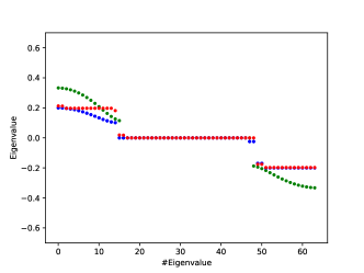
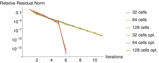
Figure 2: Solving $-\Delta u=1$ in 1D with Dirichlet boundary conditions. Left: eigenvalues of the error operator $E$, for a 32-cell mesh. Green: optimizing $\alpha$ for $\delta_{0}=2$ (classical choice). Blue: optimizing $\alpha$ and $\delta_{0}$. Red: optimizing $\alpha$, $\delta_{0}$ and $c$. Right: GMRES iterations for classical interpolation $c=0.5$, with $\delta_{0}=2$ and $\alpha=8/9$, and for the optimized clustering choice, leading to finite step convergence.

the eigenvalues of the iteration operator for a 32-cell mesh in 1D with Dirichlet boundary conditions, for continuous interpolation and $\delta_{0}=2$ optimizing only $\alpha$, optimizing both $\alpha$ and $\delta_{0}$, and the optimized clustering choice. We clearly see the clustering of the eigenvalues, including some extra clusters due to the Dirichlet boundary conditions. We also note that the spectrum is nearly equioscillating due to condition (1) and (2), which delivers visibly an optimal choice in the sense of minimizing the spectral radius of the error operator. With periodic boundary conditions, the spectral radius for the optimal choice of $\alpha$, $\delta_{0}$ and $c$ is $0.19732$, while only optimizing $\alpha$ and $\delta_{0}$ it is $0.2$. The eigenvalues due to the Dirichlet boundary conditions are slightly larger than $0.2$, but tests with periodic boundary conditions confirm that then these larger eigenvalues are not present. Refining the mesh conserves the shape of the spectrum shown in Fig. 2 on the left, but with more eigenvalues in each cluster, except for the clusters related to the Dirichlet boundary conditions. Note also that since the error operator is equioscillating around zero, the spectrum of the preconditioned system is equioscillating around one, and since the spectral radius is less than one, the preconditioned system has a positive spectrum and is thus invertible.

In Fig. 2 on the right we show the GMRES iterations needed to reduce the residuals by $10^{-8}$ for different parameter choices and the clustering choice, for different mesh refinements. We observe that the GMRES solver becomes exact after six iterations for the clustering choice.

We next perform tests in two dimensions using an interpolation operator with a stencil that is simply a tensor product of the 1D stencil $\left(\begin{smallmatrix}1&0\\ c&1-c\\ 1-c&c\\ 0&1\end{smallmatrix}\right)\otimes\left(\begin{smallmatrix}1&0\\ c&1-c\\ 1-c&c\\ 0&1\end{smallmatrix}\right)$, where $\otimes$ stands for the Kronecker product. This is very common in DG methods where even the cell block-Jacobi matrix can be expressed as a Kronecker sum for fast inversion. We show in Fig. 3

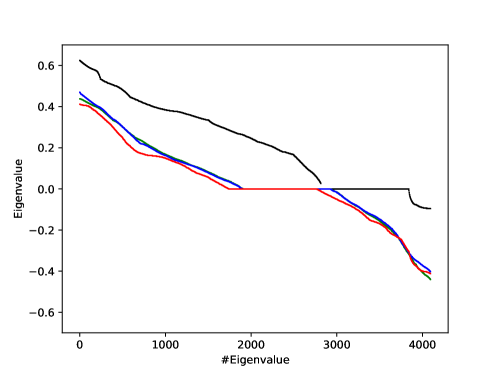
Figure 3: Spectrum of the iteration operator for a 32-by-32 square 2D mesh. Black: optimizing $\alpha$ for $\delta_{0}=2$ (classical choice) in 1D. Green: optimizing $\alpha$ and $\delta_{0}$ in 1D. Blue: optimizing $\alpha$, $\delta_{0}$ and $c$ in 1D. Red: numerically optimizing $\alpha$, $\delta_{0}$ and $c$ in 2D.

the spectrum for different optimizations in two dimensions. We observe that the clustering is not present, however as shown in detail in GanderLucero2020 for classical interpolation, the optimal choice from the 1D analysis is also here very close to the numerically calculated optimum in 2D.

4 Conclusion

We studied the question whether in two level methods for DG discretizations one should use a discontinuous interpolation operator. Our detailed analysis of a one dimensional model problem showed that the optimization of the entire two level process indeed leads to a discontinuous interpolation operator, and the performance of this new two level method is superior to the case with the continuous interpolation operator. More importantly however, the discontinuous interpolation operator allowed us to cluster the spectrum for our model problem, which then permits a Krylov method with this preconditioner to become a direct solver, converging in the number of iterations corresponding to the number of clusters in exact arithmetic. Our numerical experiments showed that this is indeed the case, but that when using the one dimensional optimized parameters in higher spatial dimensions, the spectrum is not clustered any more. Nevertheless, the 1D parameters lead to a two level performance very close to the numerically optimized one in 2D. We are currently investigating if there is a choice of interpolation operator in 2D which still would allow us to cluster the spectrum, and what the influence of this discontinuous interpolation operator is on the Galerkin coarse operator obtained.

References

• [1] Paola F. Antonietti, Marco Sarti, and Marco Verani. Multigrid algorithms for hp-discontinuous Galerkin discretizations of elliptic problems. SIAM Journal on Numerical Analysis, 53(1):598–618, 2015.
• [2] Douglas N. Arnold. An interior penalty finite element method with discontinuous elements. SIAM J. Numer. Anal., 19(4):742–760, 1982.
• [3] Michele Benzi, Martin J. Gander, and Gene H. Golub. Optimization of the hermitian and skew-hermitian splitting iteration for saddle-point problems. BIT Numerical Mathematics, 43(5):881–900, 2003.
• [4] Achi Brandt. Multi-level adaptive solutions to boundary-value problems. Mathematics of Computation, 31(138):333–390, 1977.
• [5] Maksymilian Dryja and Piotr Krzyżanowski. A massively parallel nonoverlapping additive Schwarz method for discontinuous Galerkin discretization of elliptic problems. Numerische Mathematik, 132(2):347–367, February 2016.
• [6] R. P. Fedorenko. The speed of convergence of one iterative process. Zh. Vychisl. Mat. Mat. Fiz., 4:559–564, 1964.
• [7] X. Feng and O. Karakashian. Two-level non-overlapping Schwarz methods for a discontinuous Galerkin method. SIAM J. Numer. Anal., 39(4):1343–1365, 2001.
• [8] Martin Jakob Gander and José Pablo Lucero Lorca. Optimization of two-level methods for DG discretizations of reaction-diffusion equations, 2020.
• [9] P. Hemker. Fourier analysis of grid functions, prolongations and restrictions. Report NW 98, CWI, Amsterdam, 1980.
• [10] P. Hemker, W. Hoffmann, and M. van Raalte. Two-level fourier analysis of a multigrid approach for discontinuous Galerkin discretization. SIAM Journal on Scientific Computing, 3(25):1018–1041, 2003.
• [11] P. W. Hemker, W. Hoffmann, and M. H. van Raalte. Fourier two-level analysis for discontinuous Galerkin discretization with linear elements. Numerical Linear Algebra with Applications, 5 – 6(11):473–491, 2004.
• [12] David Silvester and Andrew Wathen. Fast iterative solution of stabilised Stokes systems part II: Using general block preconditioners. SIAM Journal on Numerical Analysis, 31(5):1352–1367, 1994.