Experimental Mathematics Approach to Gauss Diagrams Realizability

Abstract

A Gauss diagram (or, more generally, a chord diagram) consists of a circle and some chords inside it. Gauss diagrams are a well-established tool in the study of topology of knots and of planar and spherical curves. Not every Gauss diagram corresponds to a knot (or an immersed curve); if it does, it is called realizable. A classical question of computational topology asked by Gauss himself is which chords diagrams are realizable. An answer was first discovered in the 1930s by Dehn, and since then many efficient algorithms for checking realizability of Gauss diagrams have been developed. Recent studies in [GL18, GL20] and [Bir19] formulated especially simple conditions related to realizability which are expressible in terms of parity of chords intersections. The simple form of these conditions opens an opportunity for experimental investigation of Gauss diagrams using constraint satisfaction and related techniques. In this paper we report on our experiments with Gauss diagrams of small sizes (up to 11 chords) using implementations of these conditions and other algorithms in logic programming language Prolog. In particular, we found a series of counterexamples showing that that realizability criteria in [GL18, GL20] and [Bir19] are not completely correct.

1 Introduction

Gauss words and Gauss diagrams are natural combinatorial encodings of generic smooth closed planar curves. For a closed planar curve its Gauss code (word) can be obtained by first assigning different symbols to all intersection points and then by writing down the symbols of intersection points passed over during traversal of the curve, starting and finishing at the chosen non-intersection point, see (Fig 1, a). The Gauss code of a closed curve with $n$ intersection points has a length $2n$ and it is a double occurrence word, that is in which each symbol occurs twice. With any double occurrence word one can further associate its chord (or Gauss) diagram which consists of a circle with all symbols of the word placed at the points of the circle following its clockwise traversal. The chords of the diagram link the points labelled by the same symbol, (Fig.1,b). Not every double occurrence word and its Gauss diagram correspond to (can be obtained from) a closed planar curve; if they do, they are called realizable.

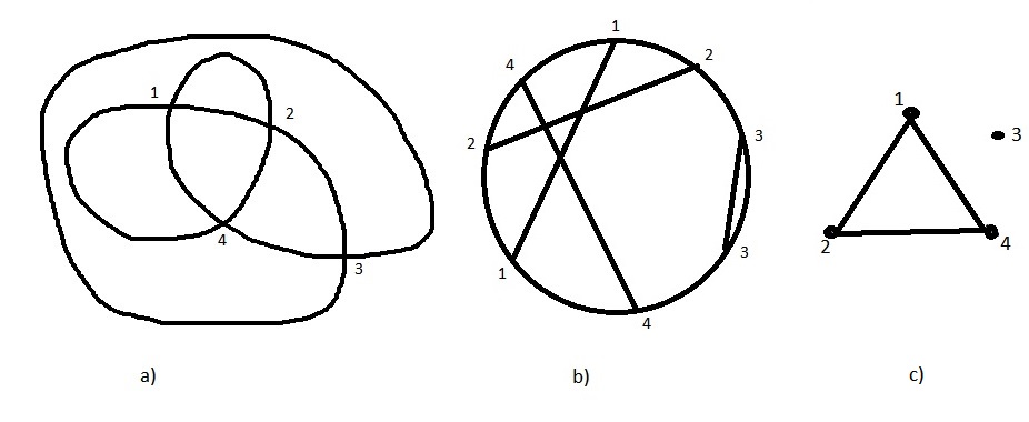
Figure 1: Example of a) a planar curve; b) its Gauss diagram and c) its interlacement graph. The corresponding Gauss word is 12334124

A classical question of computational topology asked by Gauss [Gau00] is which of the chords diagrams are realizable. Gauss himself gave a partial answer in terms of a necessary condition - in a realizable diagram any chord intersects even number of other chords Additional necessary condition was provided by Nagy [Nag27] and a full answer to Gauss’ question was discovered in the 1930s by Dehn [Deh36]. Since then many efficient criteria and algorithms for checking the realizability of Gauss diagrams have been developed [Mar69, Fra69, de 81, LM76, Ros76, RR76, RT84, dFOdM97, DT83, Ven18, CE96, CW94]. As computational complexity concerned recognition of realizability of Gauss diagrams or words can be done in polynomial time and even in linear time [RT84]. Furthermore as it is shown in [LPS11] it can be done with logarithmic space complexity. All realizability criteria and detection algorithms in the papers cited above can be expressed in terms of a diagram graph $(V,E,H)$ with two types of edges representing a chord diagram. Vertices of the graph are points of the diagrams, one type $E$ of edges corresponds to chords, the edges of another type $H$ form a cycle covering all vertices in $V$, see Fig. 2.

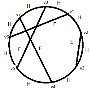
Figure 2: Diagram graph of the diagram from Fig 1, b)

With every Gauss diagram one may further associate an interlacement graph whose vertices are the chords of the diagram and two vertices are adjacent if an only if the corresponding chords intersect, see (Fig. 1, c). The interlacement graph of a diagram embodies an essential information about its realiziability. Furthermore, as it was shown in [Ros76, dFOdM97, STZ09] the realizability of Gauss diagrams can be decided based on their interlacement graphs only. The criteria are more abstract then those defined in terms of diagram graphs, as different (non-isomorphic) diagram graphs may have isomorphic corresponding interlacement graphs. At the same time criteria from [Ros76, dFOdM97, STZ09] appear to be computationally more costly. Some account of this can be given in terms of definability and descriptiive complexity [Imm99]. The formal definition of these conditions can be presented in first-order logic (FO) extended by a parity quantifier (${\rm MOD_{2}}$) [Nur00] and monadic second-order quantification (MSO). While parity quantifier evaluation can be implemented very efficiently, second-order quantification goes over all subsets of vertices. Hence checking these conditions by a straightforward algorithm requires exponential time. More recent studies [GL18, GL20, Bir19] formulated even simpler realizability conditions expressible in terms of the interlacement graphs. In particular [GL18, GL20] proposed a criteria based on parity conditions and reduction operation on the graph, while [Bir19] reformulated it in a simple form, expressed in ${\rm FO+MOD_{2}}$. Further simple analysis shows that the original conditions from [GL18] can be expressed in ${\rm FO+MOD_{2}}$ too. Hence both variants of criteria can be tested in polynomial time and logarithmic space. Furthermore the simple and declarative form of these conditions opens an opportunity for experimental investigation of Gauss diagrams using constraint satisfaction [Tsa93, RBW06] and related computational techniques. We took this opportunity as a starting point of our research in experimental mathematics with the primary aim to enumerate various classes of Gauss diagrams. We have implemented the declarative realizability conditions and algorithms from [Bir19], [GL20] and [STZ09] alongside with the classical algorithm from [Deh36] (for the latter see detailed exposition in e.g. [Kau99]). We have enumerated several interesting classes of Gauss diagrams up to sizes 10-12 (number of chords), confirming and expanding on known enumerations (for the latter see e.g. [CZ16] and references therein). The detailed presentation of this will be given in an extended version of this paper. In the present note we confine ourselves with the presentation of the most surprising discovery, that is the realiziability conditions in [Bir19], [GL20] are not completely correct. We present a minimal counterexample to both conditions of size 9 and enumerate all countexamples of sizes 10 and 11. We further confirm experimentally up to the size 11 that criteria from [Bir19] and [GL20] are equivalent, and the condition from [STZ09] is correct, i.e equivalent to that from [Deh36].

2 Preliminaries

In this section we formally discuss the definitions used in our paper.

Definition 1

[Car91] Immersed into a surface G curve is a mapping $\gamma:S^{1}\rightarrow G$. Two curves $\gamma_{1}$ and $\gamma_{2}$ are geotopic [Car91], or just equivalent if there is a homeomorphism $h:G\rightarrow G$ such that $h\gamma_{1}=\gamma_{2}$.

In this paper we are only concerned with the curves immersed into plane $R^{2}$ or sphere $S^{2}$.

Definition 2

A word is called double occurrence if each letter appears exactly twice in it. With every double occurrence word $w=a_{0}a_{1}\ldots a_{2n-1}$, one can associate a Gauss diagram $g(w)=\langle V,E,H\rangle$ , that is an undirected graph with two types of edges. Here the set of vertices $V=\{i\mid 0\leq i\leq 2n-1\}$, the set of edges called chords $E=\{(i,j)\mid i<j\;\&\;a_{i}=a_{j}\}$, and set of edges $H=\{(i,j)\mid j=i+1\;mod\;2n\}$ which form a cycle .

Definition 3

An abstract Gauss diagram is a finite undirected graph $\langle V,E,H\rangle$ with the set of vertices $V$ and two types of edges $E$ and $H$ such that $E$ is a perfect matching on $V$ (i.e. each vertex has exactly one neighbour in $E$), and $H$ forms a simple cycle covering all vertices in $V$. We will occasionally omit the qualifier word “abstract” for Gauss diagrams when it is clear from the context and/or does not lead to the confusion.

Definition 4

Given a Gauss diagram $g=\langle V,E,H\rangle$, the interlacement graph $I_{g}$ of $g$ is an undirected graph $\langle V_{I},E_{I}\rangle$, where the set of vertices $V_{I}$ is the set of edges $E$ of $g$, and $((i,j),(k,l))\in E_{I}$ iff the edges $(i,j)$ and $(k,l)$ are interlaced in $g$, that is either $i<k<j<l$, or $k<i<l<j$ holds true.

Definition 5

A Gauss diagram $g$ is called prime if and only if its interlacement graph $I_{g}$ is connected.

The equivalence of immersed curves with prime Gauss diagrams is captured by isomorphism of Gauss words and Gauss diagrams. Two double occurrences words over the same alphabet are isomorphic if one can be obtained from the other by any combination of cyclic shifts and reversing the word [Car91]. For immersed curves $\gamma_{1}$ and $\gamma_{2}$, such that their Gauss diagrams are prime, both corresponding Gauss words and Gauss diagrams are isomorphic if and only if $\gamma_{1}$ and $\gamma_{2}$ are equivalent, see e.g. [CHLR06].

A double occurrence word $w$ is called realizable iff there exists an immersed in a plane (or sphere $S^{2}$) curve $\gamma$, such that $w$ is associated with $\gamma$. A Gauss diagram $g$ is realizable iff there is a realizable word $w$ such that $g$ is isomorphic to $g(w)$.

Not all double occurrences words and Gauss diagram are realizable. In this paper we mainly focus on investigation of the realizability criteria of prime Gauss diagrams expressed solely in terms of their interlacement graphs.

One necessary realizability condition proposed by Gauss himself can be formulated in terms of interlacement graphs as follows:

C1: If a Gauss diagram $g$ is realizable then in its interlacement graphs $I_{g}$ every node has an even degree.

3 Realizability criteria based on interlacement graphs

In this section we overview known realiziability criteria for Gauss diagrams, which are defined in terms of the interlacement graphs.

3.1 R-conditions

For the first time relizability criteria for Gauss words and diagrams expressed solely in terms of interlacement graphs have been established by Rozentiehl in [Ros76]. Following [dFOdM97] Rozentiehl’s conditions can be formulated as follows. A Gauss diagram $g$ is realizable iff its interlacement graph $I_{g}$ has the following properties:

• $I_{g}=(V,E)$ is eulerian, that is each vertex has an even degree;         (C1)

• there is a subset of vertices $A\subset V$ of $I_{g}$ such that the following two conditions are equivalent for any two vertices $u$ and $v$:

  • the vertices u and v have an odd number of common neighbours,

  • the vertices u and v are neighbours and either both are in $A$ or neither is in $A$

3.2 STZ-conditions

Shtylla, Traldi and Zulli in [STZ09], while keeping C1 condition, presented an algebraic re-formulation of the second Rosentiehl’s condition:

• For its adjacency matrix $M_{g}$ there is a diagonal matrix $\Lambda_{g}$ such that $M_{g}+\Lambda_{g}$ is an idempotent matrix (all matrices are considered over $GF(2)$, the finite field of two elements).

3.3 GL-conditions

Further criteria for realizability expressible in terms of interlacement graph have been presented by Grinblat and Lopatkin in [GL18, GL20]. A prime Gauss diagram $g$ is realizable if and only if the following conditions hold true:

• In its interlacement graph $I_{g}$ each pair of non-neighbouring vertices has an even number of common neighbours (possibly, zero).                   (C2)

• The above condition C2 holds true for the reduced graph $I_{g}/v$ for each vertex $v$ of $I_{g}$.

For a vertex $v$ of $I_{g}=\langle V,E\rangle$ the reduced graph $I_{g}/v=\langle V^{\prime},E^{\prime}\rangle$ is defined as follows. $V^{\prime}=V-\{v\}$ and $E^{\prime}=\{(v_{1},v_{2})\in E|((v,v_{1})\not\in E)\lor(v,v_{2})\not\in E))\}\cup\{(v_{1},v_{2})\mid(v,v_{1})\in E\;\&\;(v,v_{2})\in E\;\&\;(v_{1},v_{2})\not\in E\}$. See also further discussion of this operation in terms of intersecting chords in Section 2 of [Bir19].

3.4 B-conditions

Biryukov in [Bir19] presents even simpler than GL-conditions realizability criteria explicitly expressed in terms of interlacement graph: A prime Gauss diagram $g$ is realizable if and only if the following conditions for $I_{g}=\langle V,E\rangle$ hold true:

• It satisfies both above C1 and C2 conditions, which amounts to strong parity condition from [Bir19];

• For any three pairwise connected vertices $a,b,c\in V$ the sum of the number of vertices adjacent to $a$, but not adjacent to $b$ nor $c$, and the number of vertices adjacent to b and c, but not adjacent to $a$, is even.                   (B3)

3.5 Remarks on definability and complexity

$R$- and $STZ$- conditions use explicit second order-quantifier “there exists a subset A” and can be defined over $I_{g}$ in monadic second order logic extended by a parity quantifier (${\rm MSO+MOD_{2}}$). That implies the exponential time upper bound for computational complexity of their checking. B-conditions on the other hand don’t use second-order quantification and can be defined in first-order logic extended by parity quantifier (${\rm FO+MOD_{2}}$). For example, the definition for (B3) is:

$$\forall x,y,z((E(x,y)\land E(x,z)\land E(y,z)\Rightarrow$$

$$\exists^{even}w((E(x,w)\land\neg E(y,w)\land\neg E(z,w)\land(y\not=w)\land(z\not=w))$$

$$\lor(\neg E(x,w)\land E(y,w)\land E(z,w)\land(x\not=w))))$$

Here $E(\_,\_)$ refers to (interpreted by) the edges of the interlacement graph and $\exists^{even}w$ is parity quantifier meaning “there exists an even number of elements/valuations of $w$ such that $\ldots$”. ${\bf C2}$ condition can be defined in a similar way. Furthermore, using locality property of the reduction operation, the second GL condition can also be defined in ${\rm FO+MOD_{2}}$. Thus, both B and GL conditions can be checked with logarithmic space (and polynomial time) complexity [Imm99].

4 Lintels

We aim to implement efficient algorithms for generating Gauss diagrams, checking their (non-)equivalence, listing all non-equivalent diagrams, satisfying combinations of criteria and checking the realiziability criteria. As a starting point we take Definition 2, and consider the generation of Gauss diagrams with a sets of vertices $V=\{i\mid 0\leq i\leq 2n-1\}$ for some $n\geq 2$ satisfying an additional constraint, corresponding to the condition C1. For that we introduce a concept of lintel, and useful algorithms working on lintels.

Let $n$ be a positive integer. A lintel is an $n$-tuple of pairs of numbers $((a^{1}_{1},a^{2}_{1}),\dots,$ $(a^{1}_{n},a^{2}_{n}))$ such that 1) the set of numbers in the lintel $\{a^{1}_{i},a^{2}_{i},\dots,a^{1}_{n},a^{2}_{n}\}$ is equal to the set $\{0,1,\dots,2n-1\}$, and 2) in each pair $(a^{1}_{i},a^{2}_{i})$ the difference $a^{1}_{i}-a^{2}_{i}$ is odd. The number $n$ will be called the size of the lintel. Each pair $(a^{1}_{i},a^{2}_{i})$ will be called a chord of the lintel.

For example, $L=((4,7),(8,1),(5,0),(2,9),(6,3))$ is a lintel of size $5$. For better readability, below we will write the two numbers in each chord under one another; therefore, the lintel $L$ can be written as $\begin{pmatrix}4&8&5&2&6\\ 7&1&0&9&3\end{pmatrix}$.

Let us say that two lintels are strongly equivalent if they can be transformed into one another by steps of the following two types:

1. Swapping the positions of two numbers in a chord; for example, the lintel $L$ in the example above is strongly equivalent to $\begin{pmatrix}4&8&0&2&6\\ 7&1&5&9&3\end{pmatrix}$;

2. Swapping the positions of chords in the list; for example, the lintel $L$ in the example above is strongly equivalent to $\begin{pmatrix}2&8&5&4&6\\ 9&1&0&7&3\end{pmatrix}$.

Among the lintels that are strongly equivalent to each other, one can point at one which can serve as the canonical lintel of this class of lintels. To define it, let us introduce a kind of lexicographic order on lintels. Consider two lintels of size $n$, $L=\begin{pmatrix}a^{1}_{1}&\dots&a^{1}_{n}\\ a^{2}_{1}&\dots&a^{2}_{n}\end{pmatrix}$ and $M=\begin{pmatrix}b^{1}_{1}&\dots&b^{1}_{n}\\ b^{2}_{1}&\dots&b^{2}_{n}\end{pmatrix}$. We will say that $L$ is less than $M$ if there is a position $i$ such that $a^{1}_{j}=b^{1}_{j}$ and $a^{2}_{j}=b^{2}_{j}$ for all $j<i$, and either $a^{1}_{i}<b^{1}_{i}$, or $a^{1}_{i}=b^{1}_{i}$ and $a^{2}_{i}<b^{2}_{i}$. We will call this order the L-order. The lintel which is the least one relative to the L-order among the lintels that are strongly equivalent to each other will be treated as the canonical representative of this class of lintels. There is also another way to define this lintel. Let us say that a lintel is a sorted lintel if each pair in it is sorted, and first elements of pairs are sorted, that is, for each $i$ we have $a^{1}_{i}<a^{2}_{i}$, and for all $i<j$ we have $a^{1}_{i}<a^{1}_{j}$. In each class of lintels that are strongly equivalent to each other, there is exactly one sorted lintel, and it is the one that is the least one relative to the L-order. For a given lintel $L$, one can produce the sorted lintel corresponding to $L$ using the following simple algorithm.

Algorithm 1

1. Sort the two numbers in each chord.
2. Sort all the chords by the values of their first entry.

Let us say that two lintels are equivalent if they can be transformed into one another by steps of the following types:

1. the two types of steps defining strongly equivalent lintels

2. shifting the value of each entry of the lintel cyclically modulo $2n$, that is, replacing a lintel $\begin{pmatrix}a^{1}_{1}&\dots&a^{1}_{n}\\ a^{2}_{1}&\dots&a^{2}_{n}\end{pmatrix}$ by a lintel $\begin{pmatrix}a^{1}_{1}+s&\dots&a^{1}_{n}+s\\ a^{2}_{1}+s&\dots&a^{2}_{n}+s\end{pmatrix}$ for some value $s$, with operations performed in the arithmetic modulo $2n$;

3. inverting the value of each entry of the lintel modulo $2n$, that is, replacing a lintel $\begin{pmatrix}a^{1}_{1}&\dots&a^{1}_{n}\\ a^{2}_{1}&\dots&a^{2}_{n}\end{pmatrix}$ by the lintel $\begin{pmatrix}-a^{1}_{1}&\dots&-a^{1}_{n}\\ -a^{2}_{1}&\dots&-a^{2}_{n}\end{pmatrix}$, with operations performed in the arithmetic modulo $2n$;

Now we are ready to define a canonical lintel. Namely, the lintel which is the least one relative to the L-order among the lintels that are equivalent to each other will be treated as the canonical representative of this class of lintels We shall call such lintels Lyndon lintels. This construction is similar in certain aspects to Lyndon words in algebra, hence the name Obviously, a Lyndon lintel is a sorted lintel, but not every sorted lintel is a Lyndon lintel. For a given lintel $L$, one can produce the sorted lintel corresponding to $L$ using the following algorithm.

Algorithm 2

1. Produce the sorted lintel $M$ corresponding to $L$.
2. Applying cyclic shifts to $M$ for all values $s=1,\dots,2n-1$, produce lintels $L_{s}$.
3. Produce the sorted lintels $M_{s}$ corresponding to $L_{s}$.
4. Applying the inverting step to $L$, produce the lintel $L^{\prime}$.
5. Produce the sorted lintel $M^{\prime}$ corresponding to $L^{\prime}$.
6. Applying cyclic shifts to $M^{\prime}$ for all values $s=1,\dots,2n-1$, produce lintels $L^{\prime}_{s}$.
7. Produce the sorted lintels $M^{\prime}_{s}$ corresponding to $L^{-}_{s}$.
8. Among the sorted lintels $M,M^{\prime},L_{s},L^{\prime}_{s}$, choose the least one relative to the L-order.

Proposition 1

The number of equivalence classes for strong equivalence relation on lintels of size $n$ is $n!$

Proof Let $I_{2n}=\{0,\ldots,2n-1\}$. Denoted by $P_{2n}$ the set of all even-odd matchings of $I_{2n}$, that is partitions of $I_{2n}$ into subsets of size 2, each containing one even and one odd number. The obvious consequence of definitions is that elements of $P_{2n}$ are in bijective correspondence with the set of all equivalence classes for strong equivalence relation on lintels of size $n$. Now for symmetric group $S_{n}$ we define a mapping $\beta:S_{n}\rightarrow P_{2n}$ as follows. For $\sigma\in S_{n}$, $\sigma:[1..n]\rightarrow[1..n]$ $\beta(\sigma)=\{\{2*i-1,2*\sigma(i)-2\}|i\in[1..n]\}$. Straightforward check shows that $\beta$ is a bijection between $S_{n}$ and $P_{2n}$.

Note 1

The fact $|P_{2n}|=n!$ is mentioned (without the reference to the proof) in OEIS article A000142 [oeia] with an attribution to David Callan, Mar 30 2007. We use explicit simple bijection between $P_{2n}$ and $S_{n}$ for the efficient generation of lintels.

5 Implementation

We have implemented the algorithms suite Gauss-Lint for Gauss diagram generation, equivalence checking, canonization, and realizability conditions using the concept of lintels. The prototype implementation in logic programming language SWI-Prolog [WSTL12] is available at [KLV21].

Here we give a short overview of the implementation while more detailed presentation is deferred to the extended version of this paper.

5.1 Essential feature

As we use lintel concept/data structure, all generated Gauss diagrams in our implementation satisfy condition ${\bf C1}$.

5.2 Data structures

We utilise a list of lists representation of lintels in Prolog. As an example, Prolog list [[0,3],[1,4],[2,5]] represents a lintel $\begin{pmatrix}0&1&2\\ 3&4&5\end{pmatrix}$.

5.3 Dynamic facts

We use dynamic facts to store intermediate and final results of computations. E.g. a dynamic fact “lintel(Size,L)” stores a generated canonical lintel satisfying some conditions (depending on the user’s choice).

5.4 Lintel generation and canonization

The canonical lintel generation is based on efficient built-in Prolog predicate permutation(X,Y) for the generation of all permutations of a given list (assigned to) $X$ and the use of bijection $\beta:S_{n}\rightarrow P_{2n}$ (Section 4).

The generic generation process proceeds as follows. Once a permutation $\sigma$ is generated, the bijection $\beta$ is applied to it, and then the Algorithm 2 is applied to $\beta(\sigma)$. The resulted canonical lintel then checked on

• whether it satisfies chosen combination of conditions;

• whether it has not been stored yet as a dynamic fact.

If both conditions are satisfied then the lintel is added as a dynamic fact, and the process is backtracked to the generation of the new permutation. When no new permutations are left, the database of dynamic facts provides a list of all canonical non-equivalent lintels of given size satisfying chosen combination of properties.

5.5 Properties/conditions checking

We have implemented the checking of following properties/conditions of Gauss diagrams presented in lintel format: primality, C2, STZ, B, GL. As mentioned before, C1 is satisfied automatically for diagrams presented by lintels. We have also implemented a classical algorithm (CA) for realiziability checking from [Deh36, Kau99].

6 Experiments and Counterexamples

Using our implementation we have conducted various experiments and enumerated the classes of non-equivalent Gauss diagrams, satisfying various combinations of properties.

	3	4	5	6	7	8	9	10	11
Realisability (CA)	1	1	2	3	10	27	101	364	1610
STZ	1	1	2	3	10	27	101	364	1610
B	1	1	2	3	10	27	102	370	1646
GL	1	1	2	3	10	27	102	370	1646

Table 1: The number of non equivalent Gauss diagrams of sizes = 3, …, 11, satisfying various realizability conditions

Table 1 shows the numbers of non-equivalent Gauss diagrams of sizes $3\ldots 11$ satisfying different realizability conditions, generated by our program. The first two lines, found also in OEIS article A264759 [oeib], together with the fact that generated corresponding lists of Gauss diagrams are the same, verify that indeed, STZ are correct realizability conditions up to the size 11.

The last two lines show an interesting phenomenon. Up to the size 8 B and GL conditions are satisfied by the same diagrams, as CA and STZ are. For the size 9, however, there is one (= $102-101$) up to equivalence Gauss diagram such that it satisfies both B and GL conditions, but still is not realizable. For sizes 10 and 11 the numbers of such diagrams are 6 and 36, respectively.

In summary, CA and STZ, respectively B and GL, are pairwise equivalent conditions up to the size 11. B and GL, however are not equivalent to CA or STZ, starting from size 9. Hence B and GL are not correct realizability criteria despite the claims in [Bir19] and [GL18, GL20], respectively.

Counterexample, Size=9

The lintel

[[0,5],[1,8],[2,9],[3,14],[4,15],[6,13],[7,12],[10,17],[11,16]]

represents a minimal and single up to equivalence non-realizable Gauss diagram of size 9, satisfying both B and GL conditions, Fig 3.

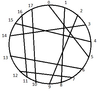
Figure 3: Minimal counterexample, n=9

Counterexamples, Size=10

The following lintels represent all six up to equivalence non-realizable Gauss diagrams of size 10 satisfying both B and GL conditions, Fig 4.

[[0,3],[1,10],[2,9],[4,15],[5,16],[6,19],[7,14],[8,13],[11,18],[12,17]]
[[0,3],[1,8],[2,9],[4,15],[5,16],[6,13],[7,12],[10,17],[11,18],[14,19]]
[[0,3],[1,10],[2,9],[4,17],[5,16],[6,11],[7,14],[8,15],[12,19],[13,18]].
[[0,3],[1,8],[2,9],[4,17],[5,16],[6,13],[7,14],[10,15],[11,18],[12,19]].
[[0,5],[1,10],[2,15],[3,16],[4,9],[6,13],[7,14],[8,19],[11,18],[12,17]].
[[0,5],[1,16],[2,15],[3,10],[4,9],[6,19],[7,14],[8,13],[11,18],[12,17]].

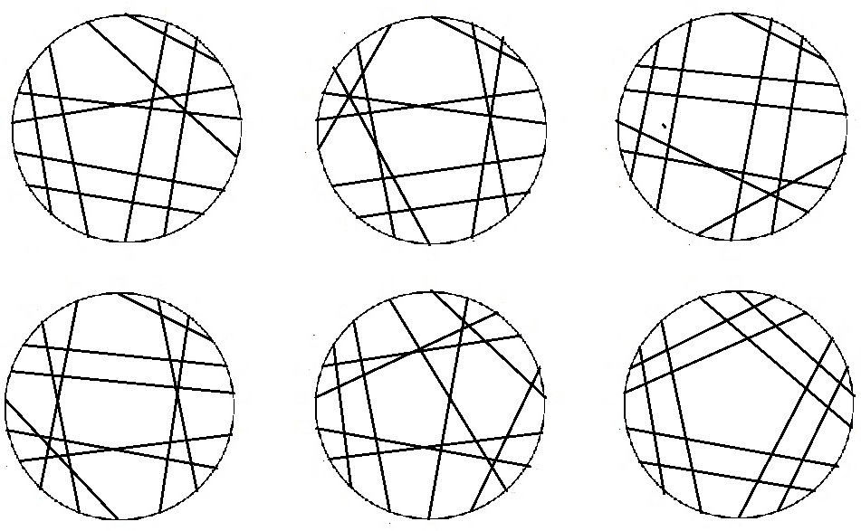
Figure 4: All counterexamples for n=10

7 Conclusion

We have presented an approach to experimental investigation of Gauss realizability conditions based on the concept of lintel. We have implemented the algorithms for Gauss diagrams generation, canonization and checking recently proposed declarative criteria for Gauss realizability. We reported on the experiments with our implementations and presented counterexamples for the recently published simple realizability criteria. Based on that we conjecture that realizability of Gauss diagrams can not be defined in first-order logic with parity quantifier over their interlacement graphs.

References

- [Bir19] Oleg N. Biryukov. Parity conditions for realizability of Gauss diagrams. Journal of Knot Theory and Its Ramifications, 28(01):1950015, 2019.
- [Car91] J. Scott Carter. Classifying immersed curves. Proc. Amer. Math. Soc., 111(1):281–287, 1991.
- [CE96] Grant Cairns and Daniel M. Elton. The planarity porblem II. J. Knot Theory Ramif., 5(2):137–144, 1996.
- [CHLR06] Michael Chmutov, Thomas Hulse, Andrew Lum, and Peter Rowell. Plane And Spherical Curves: An Investigation of Their Invariants. In Research Experiences for Undergraduates (REU), Summer Mathematics Research Institute, REU 2006 Proceedings, Oregon State University, 2006.
- [CW94] Nathalie Chaves and Claude Weber. Plombages de rubans et problème des mots de Gauss. Expo. Math., 12:53–77, 1994.
- [CZ16] Robert Coquereaux and Jean-Bernard Zuber. Maps, immersions and permutations. J. Knot Theor. Ramifications, 25(08):1650047, 2016.
- [de 81] Hubert de Fraysseix. Local complementation and interlacement graphs. Discrete Mathematics, 33(1):29 – 35, 1981.
- [Deh36] M. Dehn. Über kombinatorische topologie. Acta Math., 67:123–168, 1936.
- [dFOdM97] H. de Fraysseix and P. Ossona de Mendez. A short proof of a Gauss problem. In Giuseppe DiBattista, editor, Graph Drawing, pages 230–235, Berlin, Heidelberg, 1997. Springer Berlin Heidelberg.
- [DT83] C.H. Dowker and Morwen B. Thistlethwaite. Classification of knot projections. Topology and its Applications, 16(1):19 – 31, 1983.
- [Fra69] George K. Francis. Null genus realizability criterion for abstract intersection sequences. Journal of Combinatorial Theory, 7(4):331 – 341, 1969.
- [Gau00] Carl F. Gauss. Werke, volume VII. Tuebner, Leipzig, 1900.
- [GL18] Andrey Grinblat and Viktor Lopatkin. On realizability of Gauss diagrams and constructions of meanders. arXiv:1808.08542, 2018.
- [GL20] Andrey Grinblat and Viktor Lopatkin. On realizabilty of Gauss diagrams and constructions of meanders. Journal of Knot Theory and Its Ramifications, 29(05):2050031, 2020.
- [Imm99] Neil Immerman. Descriptive complexity. Graduate texts in computer science. Springer, 1999.
- [Kau99] Louis H. Kauffman. Virtual knot theory. European Journal of Combinatorics, 20(7):663 – 691, 1999.
- [KLV21] Abdullah Khan, Alexei Lisitsa, and Alexei Vernitski. Gauss-lint algorithms suite for Gauss diagrams generation and analysis, March 2021. Zenodo, 10.5281/zenodo.4574590, https://doi.org/10.5281/zenodo.4574590.
- [LM76] László Lovász and Morris L. Marx. A forbidden substructure characterization of Gauss codes. Bull. Amer. Math. Soc., 82(1):121–122, 01 1976.
- [LPS11] Alexei Lisitsa, Igor Potapov, and Rafiq Saleh. Planarity of knots, register automata and logspace computability. In Adrian-Horia Dediu, Shunsuke Inenaga, and Carlos Martín-Vide, editors, Language and Automata Theory and Applications, pages 366–377, Berlin, Heidelberg, 2011. Springer Berlin Heidelberg.
- [Mar69] Morris L. Marx. The Gauss realizability problem. Proceedings of the American Mathematical Society, 22(3):610–613, 1969.
- [Nag27] Julius v. Sz. Nagy. Über ein topologisches Problem von Gauß. Math. Z., 26(1):579–592, 1927.
- [Nur00] Juha Nurmonen. Counting modulo quantifiers on finite structures. Information and Computation, 160(1):62–87, 2000.
- [oeia] The On-Line Encyclopedia of Integer Sequences. http://oeis.org/A000142.
- [oeib] The On-Line Encyclopedia of Integer Sequences. http://oeis.org/A264759.
- [RBW06] Francesca Rossi, Peter van Beek, and Toby Walsh. Handbook of Constraint Programming (Foundations of Artificial Intelligence). Elsevier Science Inc., USA, 2006.
- [Ros76] Pierre Rosenstiehl. Solution algébrique du problème de Gauss sur la permutation des points d’intersection d’une ou plusieurs courbes fermées du plan. C.R. Acad. Sci., t. 283, série A:551–553, 1976.
- [RR76] Pierre Rosenstiehl and R.C. Read. On the Gauss crossing problem. In A.Hajnal and V.T. Sos eds., editors, On the Gauss crossing problem, volume II, pages 843–876, Hungary, June 1976.
- [RT84] Pierre Rosenstiehl and Robert Endre Tarjan. Gauss codes, planar hamiltonian graphs, and stack-sortable permutations. J. Algorithms, 5(3):375–390, 1984.
- [STZ09] Blerta Shtylla, Lorenzo Traldi, and Louis Zulli. On the realization of double occurrence words. Discret. Math., 309(6):1769–1773, 2009.
- [Tsa93] Edward P. K. Tsang. Foundations of constraint satisfaction. Computation in cognitive science. Academic Press, 1993.
- [Ven18] Lluis Vena. A topological characterization of Gauss codes. arXiv:1808.04630, 2018.
- [WSTL12] Jan Wielemaker, Tom Schrijvers, Markus Triska, and Torbjörn Lager. SWI-Prolog. Theory and Practice of Logic Programming, 12(1-2):67–96, 2012.